Semi-Analytical Solution for a Multi-Objective TEAM Benchmark Problem

Abstract

Benchmarking is essential for testing new numerical analysis codes. Their solution is crucial both for testing the partial differential equation solvers and both for the optimization methods. Especially, nature-inspired optimization algorithm-based solvers, where is an important study is to use benchmark functions to test how the new algorithm may perform, in comparison with other algorithms or fine-tune the optimizer parameters. This paper proposes a novel semi-analytical solution of the multi-objective T.E.A.M benchmark problem. The goal of the benchmark problem is to optimize the layout of a coil and provide a uniform magnetic field in the given region. The proposed methodology was realized in the open-source robust design optimization framework Ārtap, and the precision of the solution is compared with the result of a fully hp-adaptive numerical solver: Agros-suite. The coil layout optimization was performed by derivative-free non-linear methods and the NSGA-II algorithm.

1 Introduction

This paper deals with a seemingly simple problem, where the radius of a given number of circular turns should be optimized that would generate a uniform magnetic field in the prescribed region (Fig. 1). This task forms a proposal for the multi-objective Testing Electromagnetic Analysis Methods (TEAM) benchmark problem for Pareto-optimal electromagnetic devices [1, 2, 3]. TEAM problems offer a wide variety of test problems to benchmark the new partial differential equation and numerical solvers [1, 2, 3, 4, 5, 6, 7]. Moreover, these problems are openly accessible from the website of COMPUMAG society [8].

This test problem is inspired by a bio-electromagnetic application for Magnetic Fluid Hyperthermia (MFH), where the uniform magnetic field is used to compare the magnetic properties of the different nanofluids [9, 10, 11]. The solenoid design has great importance, as a wide range of application, fields exist, starting from electric power applications [12, 13, 14, 15, 16, 17, 18, 19, 20, 21, 22, 23, 24, 25, 26, 27, 28, 29, 30, 31, 32, 33, 34], through induction heating processes [12], [24], [34, 35, 36, 37, 38, 39, 40]⁠ to other biomedical applications [1, 2, 3] in the industry. The motivation behind the development of the Artap framework [41, 42, 43]⁠ was a similar problem. To facilitate the development of the induction brazing process, where the main design question was to find a robust design optimum, where the sensitivity of the inductor shape to the manufacturing tolerances and realized controller design had to be considered together.

The following chapters of the paper propose a novel, semi-analytical solution for the dc uniform magnetic field design and description of the automatized FEM solution using the application of the Ārtap framework.The solution of this benchmark problem is twofold: validating the correctness of the results and demonstrating the applicability of the Ārtap framework.

2 Problem Description

The described problem is shown in Fig. 1. The task is to get a region (green color in Fig.,1) with a highly uniform magnetic field distribution. This magnetic field is generated by a prescribed number ($N=20$) of massive circular turns of rectangular cross-section (yellow color in Fig. 1). During the solution of the problem, we are considering only the symmetrical solutions of the problem, as other authors handled this problem [1, 2, 3].

While the dimensions of the turns and the variation of their positions in the z-direction are fixed. The height and the width parameters of the modeled conductors are 1.5 mm and 1.0 mm during the calculations. The inner radius of the turns (radii) can be varied from 5 mm to 50 mm in the $r$-direction. All turns carry a direct current of value $I$, the current density in the conductors are $J_{\phi}=2A/mm^{2}$. The width and the height of the controlled region are 5 mm in the $r$ and the $z$ directions. In this paper, the following two-goal function based multi-objective version of the task is resolved:

$$F_{1}(r)=sup_{q=1,np}|\mbox{\boldmath$B$}(r_{q},z_{q})-\mbox{\boldmath$B_{0}$}(r_{q},z_{q})|,$$ (1)

$$F_{2}(r)=\Sigma_{n}R(r_{q}),$$ (2)

where $\mbox{\boldmath$B_{0}$}=2mT$ is the aimed magnetic flux density, and $B$ is the distribution of the magnetic flux density in the field of interest. The value of $B$ is calculated in np different points of the region of interest. $F_{2}$ function represents the mass of the winding, where $n$ is the number of turns, and $R$ is a mass function, which depends on the radii.

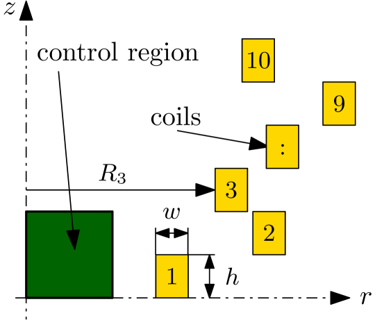
Figure 1: 2D axisymmetric model from the upper half the coil geometry and the design variables.

3 Semi-analytical Solution

Consider a single massive circular turn of rectangular cross section, see Fig. 2. The turn carries direct current $I$.

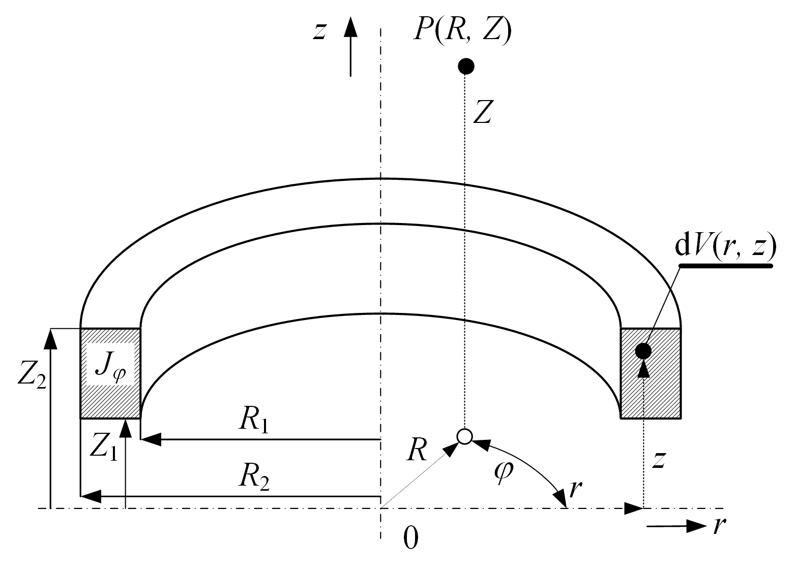
Figure 2: One, massive circular turn of rectangular cross section from the modeled solenoid coil.

Its density having only the circumferential component $J_{\varphi}$ inversely proportional to the corresponding radius $r$ is given by the formula

$$J_{\varphi}=\frac{I}{r\,(Z_{2}-Z_{1})\ln(R_{2}/R_{1})}\,.$$ (3)

The basic quantity to start with is the circumferential component $A_{\varphi}(R,Z)$ of the magnetic vector potential $A$ that is given by the formula

$$A_{\varphi}(R,Z)=\frac{\mu_{0}}{4\pi}\int_{V}\frac{J_{\varphi}\cos\varphi}{l}\,\,\mathrm{d}V\,,$$ (4)

where (see Fig. 2) $l=\sqrt{r^{2}+R^{2}-2rR\cos\varphi+(Z-z)^{2}}$ and $\,\mathrm{d}V=r\,\,\mathrm{d}r\,\,\mathrm{d}\varphi\,\,\mathrm{d}z$, $V$ denoting the volume of the ring.

The components of the magnetic flux density $B_{r}(R,Z)$ and $B_{z}(R,Z)$ at point $P(R,\,Z)$ in the directions $r$ and $z$ then follow from the relations

$$B_{r}(R,Z)=-\frac{\partial A_{\varphi}(R,Z)}{\partial Z}=\frac{\mu_{0}}{4\pi}\int_{V}\frac{J_{\varphi}(Z-z)\cos\varphi}{l^{3}}\,\,\mathrm{d}V$$ (5)

and

$$B_{z}(R,Z)=\frac{1}{R}\frac{\partial[R\,A_{\varphi}(R,Z)]}{\partial R}=$$

$$=\frac{\mu_{0}}{4\pi R}\int_{V}\frac{J_{\varphi}[r(r-R\cos\varphi)+(Z-z)^{2}]\cos\varphi}{l^{3}}\,\,\mathrm{d}V\,.$$ (6)

After substituting for ${J_{\varphi}}$ from (1), for $l$ and for $\,\mathrm{d}V$, we obtain

$$B_{r}(R,Z)=C\int_{\varphi=0}^{2\pi}\int_{r=R_{1}}^{R_{2}}\int_{z=Z_{1}}^{Z_{2}}I_{1}\,\,\mathrm{d}z\,\,\mathrm{d}r\,\,\mathrm{d}\varphi\,,$$ (7)

where

$$I_{1}=\frac{(Z-z)\cos\varphi}{\sqrt{[r^{2}+R^{2}-2rR\cos\varphi+(Z-z)^{2}]^{3}}}$$

and

$$B_{z}(R,Z)=\frac{C}{R}\int_{\varphi=0}^{2\pi}\int_{r=R_{1}}^{R_{2}}\int_{z=Z_{1}}^{Z_{2}}I_{2}\,\,\mathrm{d}z\,\,\mathrm{d}r\,\,\mathrm{d}\varphi\,,$$ (8)

where

$$I_{2}=\frac{[r(r-R\cos\varphi)+(Z-z)^{2}]\cos\varphi}{\sqrt{[r^{2}+R^{2}-2rR\cos\varphi+(Z-z)^{2}]^{3}}}\,.$$

The constant $C$ occurring in both (5) and (6) is given as

$$C=\frac{\mu_{0}I}{4\pi(Z_{2}-Z_{1})\ln(R_{2}/R_{1})}\,.$$ (9)

After the double integration with respect to $r$ and $z$, the components of the magnetic flux density are given by the formulae [44]

$$B_{r}(R,Z)=C\cdot[g(R_{2},R,Z_{2}-Z)-g(R_{2},R,Z_{1}-Z)-$$

$$-g(R_{1},R,Z_{2}-Z)+g(R_{1},R,Z_{1}-Z)]$$ (10)

and

$$B_{z}(R,Z)=C\cdot[h(R_{2},R,Z_{2}-Z)-h(R_{2},R,Z_{1}-Z)-$$

$$-h(R_{1},R,Z_{2}-Z)+h(R_{1},R,Z_{1}-Z)]\,.$$ (11)

Here, for example

$$g(R_{2},R,Z_{2}-Z)=\int_{\varphi=0}^{2\pi}\ln[R_{2}-R\cdot\cos\varphi+d_{22}]\cos\varphi\,{\rm d}\varphi\,,$$ (12)

$$h(R_{2},R,Z_{2}-Z)=-\int_{\varphi=0}^{2\pi}\ln[Z_{2}-Z+d_{22}]\,{\rm d}\varphi\,,$$ (13)

and

$$d_{22}=\sqrt{R_{2}^{2}+R^{2}-2R_{2}R\cos\varphi+(Z-Z_{2})^{2}}\,.$$ (14)

The other functions are obtained by standard interchanging of the indices. The last integrals with respect to $\phi$ are calculated using the Gauss quadrature formulae. Magnetic field produced by more turns is then given by the superposition of the partial fields produced by particular turns. The computations were realized in the Ārtap framework. It is the part of the package, which can be downloaded from the homepage of the project: http://pypi.org/project/artap .

The accuracy of the above results is compared with the results of Agros [43].

4 FEM Model

A precompiled version of the fully hp-adaptive FEM solver: Agros Suite is integrated into the Ārtap framework, and it can be invoked via a Python scripting language [41, 42]. The model geometry can be made by the aid of the user Fig. 3 The realized parametric geometry for the TEAM benchmark problem in Agros interface.

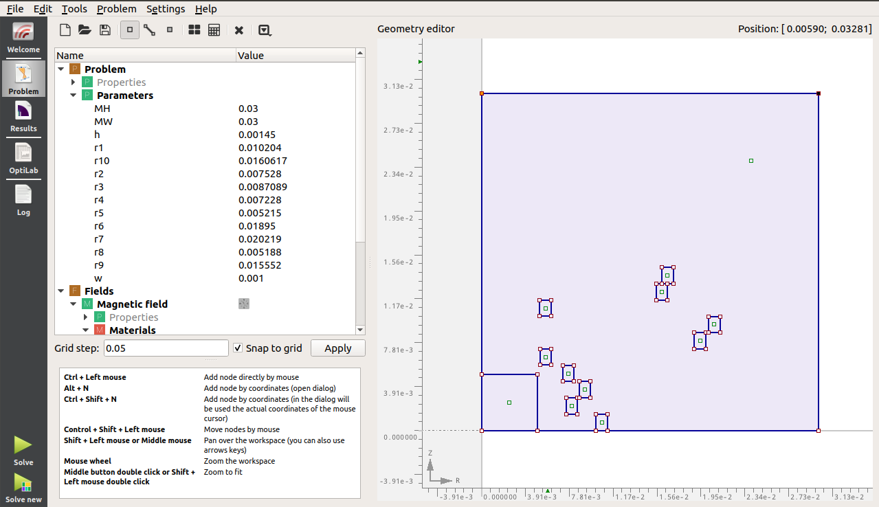
Figure 3: The realized parametric geometry for the TEAM benchmark problem in Agros.

Then we can use the ‘Create script from the model’ function of the Problem toolbar to copy the tested FEM model into the Python script (Fig. 3). This script can be inserted directly into the optimization code. The modeler has to connect the Agros model parameters with the model parameters of the Ārtap project at the beginning of the code and its ready to use.

The optimization task can be initialized by the usage of the set() function (Fig 4). Here, four parameters and methods have to be defined:

• the name of the optimization task.

• a dictionary list with the optimized parameters.

• the objective functions.

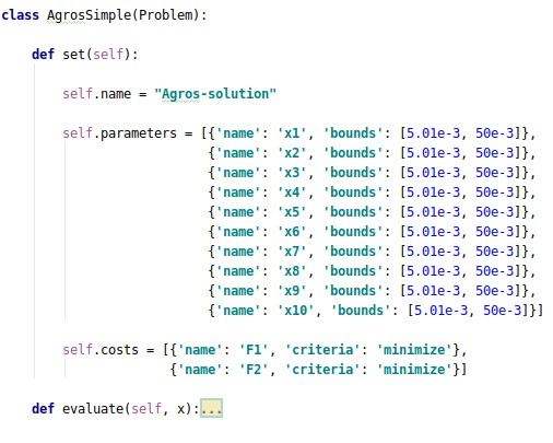
Figure 4: Initialization of the Optimization problem in Ārtap.

The exported python code has to be inserted into the evaluate() method. It gets the optimization variables via the parameter vector (x.vector) of the Individual class. This parameter introduced to the code to give the possibility to add other non-optimized, FEM or analytical results of the calculation to the Individual. These values can be saved into a database and can be post-processed after the calculation. The database management and the parallelization can be made automatically; it only has to be defined by a keyword. In this paper, we are using the NSGA-II [41, 45] algorithm to solve the optimization task. This optimization method does not need initial values, so only the name of the parameter and the lower and the upper bounds are enough for the initialization. The NSGAII algorithm is contained by the algorithm class. It is initialized by a maximum of 100 individuals in 100 generations. The realized problem can be downloaded from the project homepage, and it is part of the python package https://pypi.org/project/artap/.

5 Results and Discussion

The results of the semi-analytical calculation compared with a FEM calculation to benchmark and validate its results. For comparison, one possible turn layout is selected. Here, the radii of the turns set by the list of the x parameters: $x=[0.00808,0.0149,0.00674,0.0167,0.00545,0.0106,0.0117,0.0111,\newline 0.01369,0.00619]$. Where every value is given in m, this solenoid layout and the resulting flux density distribution is depicted in Fig 5.

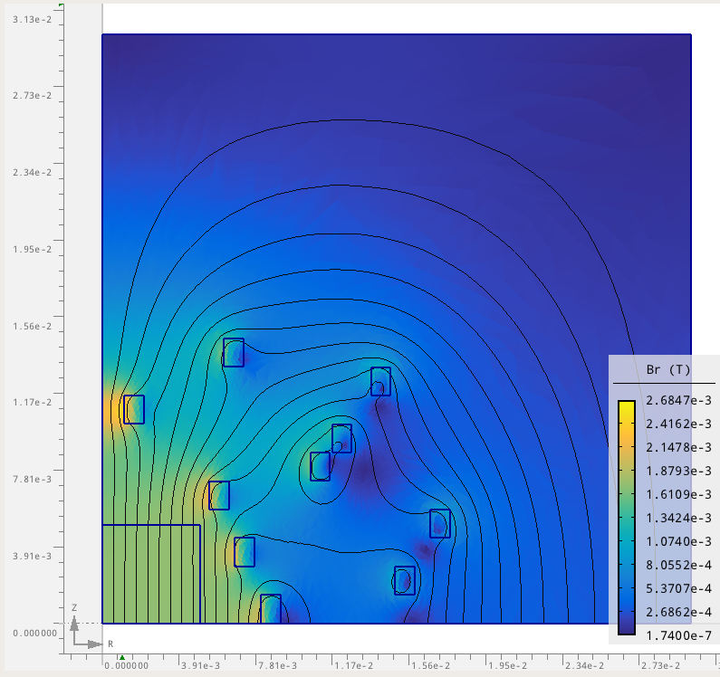
Figure 5: The examined geometry for the TEAM benchmark problem and the flux density distribution in Agros.

The radial ($B_{r}$) and the axial ($B_{z}$) components of the magnetic flux density were compared along a vertical line ($r=0.003$), where 10 different points are selected from the area of interest. The results are compared in Fig 6.

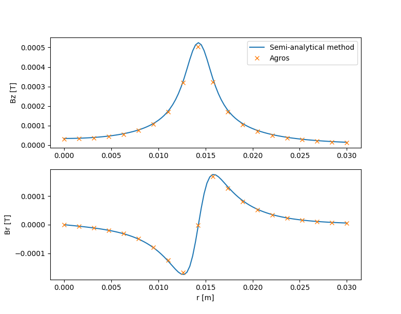
Figure 6: The $B_{r}$ and $B_{z}$ flux density components along the $x$ = 0.003 m vertical line, the values were calculated in 20 points.

As it can be seen from the results, the difference between the FEM and the semi-analytical solution is negligible. However, the computational cost of the semi-analytical calculation is much lesser than a single FEM solution. Therefore, to accelerate the optimization process, this formulation is used to search the Pareto-solutions (Fig. 7). During the calculation, 10000 iterations were performed. The shape of the resulting Pareto-front is similar to the solution, which is presented in the proposal of the benchmark problem [1, 2, 3].

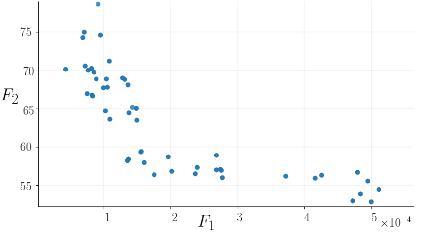
Figure 7: Last generation of the optimization for $F_{1}$ and $F_{2}$.

6 Conclusions

A novel semi-analytical solution was proposed to the multi-objective TEAM benchmark problem for electromagnetic devices. The proposed methodology was realized in the open-source robust design optimization framework Ārtap, and the precision of the solution is compared with the result of a fully hp-adaptive numerical solver: Agros-suite. The coil layout optimization was performed by derivative free non-linear optimization method, the NSGA-II algorithm. The provided semi-analytical solution can be used to test other FEM solvers and significantly reduces the calculation time of the optimization process.

References

- [1] P. Di Barba, M. E. Mognaschi, D. A. Lowther, and J. K. Sykulski, “A benchmark team problem for multi-objective pareto optimization of electromagnetic devices,” IEEE Transactions on Magnetics, vol. 54, no. 3, pp. 1–4, 2018.
- [2] P. Di Barba, F. Dughiero, M. Forzan, D. A. Lowther, M. E. Mognaschi, E. Sieni, and J. K. Sykulski, “A benchmark team problem for multi-objective pareto optimization in magnetics: The time-harmonic regime,” IEEE Transactions on Magnetics, vol. 56, no. 1, pp. 1–4, 2019.
- [3] P. Di Barba, M. E. Mognaschi, F. Dughiero, M. Forzan, and E. Sieni, “Multi-objective optimization of a solenoid for mfh: a comparison of methods,” in IECON 2018-44th Annual Conference of the IEEE Industrial Electronics Society. IEEE, 2018, pp. 3336–3340.
- [4] T. Orosz, B. Borbely, and Z. a. Tamus, “Performance comparison of multi design method and meta-heuristic methods for optimal preliminary design of core-form power transformers,” Periodica Polytechnica Electrical Engineering and Computer Science, vol. 61, no. 1, pp. 69–76, 2017.
- [5] T. Orosz, a. Sleisz, and I. Vajda, “Core-form transformer design optimization with branch and bound search and geometric programming,” in 2014 55th International Scientific Conference on Power and Electrical Engineering of Riga Technical University (RTUCON). IEEE, 2014, pp. 17–21.
- [6] A. Ben-Tal and A. Nemirovski, “Robust optimization–methodology and applications,” Mathematical programming, vol. 92, no. 3, pp. 453–480, 2002.
- [7] T. Chatterjee, R. Chowdhury, and P. Ramu, “Decoupling uncertainty quantification from robust design optimization,” Structural and Multidisciplinary Optimization, vol. 59, no. 6, pp. 1969–1990, 2019.
- [8] “Compumag - TEAM Benchmarks.”
- [9] J. Hornak, P. Trnka, P. Kadlec, O. Michal, V. Mentlik, P. Sutta, G. M. Csanyi, and Z. A. Tamus, “Magnesium oxide nanoparticles: dielectric properties, surface functionalization and improvement of epoxy-based composites insulating properties,” Nanomaterials, vol. 8, no. 6, p. 381, 2018.
- [10] S. Sun, H. Zeng, D. B. Robinson, S. Raoux, P. M. Rice, S. X. Wang, and G. Li, “Monodisperse mfe2o4 (m= fe, co, mn) nanoparticles,” Journal of the American Chemical Society, vol. 126, no. 1, pp. 273–279, 2004.
- [11] C. L. Dennis and R. Ivkov, “Physics of heat generation using magnetic nanoparticles for hyperthermia,” International Journal of Hyperthermia, vol. 29, no. 8, pp. 715–729, 2013.
- [12] D. Panek, P. Karban, T. Orosz, and I. Dolezel, “Comparison of simplified techniques for solving selected coupled electroheat problems,” COMPEL-The international journal for computation and mathematics in electrical and electronic engineering, 2020.
- [13] D. Bortis, G. Ortiz, J. W. Kolar, and J. Biela, “Design procedure for compact pulse transformers with rectangular pulse shape and fast rise times,” IEEE transactions on Dielectrics and Electrical Insulation, vol. 18, no. 4, pp. 1171–1180, 2011.
- [14] E. Mustafa, R. S. Afia, and Z. A. Tamus, “Condition monitoring uncertainties and thermal-radiation multistress accelerated aging tests for nuclear power plant cables: A review,” Periodica Polytechnica Electrical Engineering and Computer Science, vol. 64, no. 1, pp. 20–32, 2020.
- [15] T. Vajsz and L. Szamel, “Improved modified dtc-svm methods for increasing the overload-capability of permanent magnet synchronous motor servo-and robot drives–part 1,” Periodica Polytechnica Electrical Engineering and Computer Science, vol. 62, no. 3, pp. 65–73, 2018.
- [16] K. Daukaev, A. Rassolkin, A. Kallaste, T. Vaimann, and A. Belahcen, “A review of electrical machine design processes from the standpoint of software selection,” in 2017 IEEE 58th International Scientific Conference on Power and Electrical Engineering of Riga Technical University (RTUCON). IEEE, 2017, pp. 1–6.
- [17] L. Gevorkov, A. Rassolkin, A. Kallaste, and T. Vaimann, “Simulink based model of electric drive for throttle valve in pumping application,” in 2018 19th International Scientific Conference on Electric Power Engineering (EPE). IEEE, 2018, pp. 1–4.
- [18] A. Kallaste, T. Vaimann, and A. Rassolkin, “Additive design possibilities of electrical machines,” in 2018 IEEE 59th International Scientific Conference on Power and Electrical Engineering of Riga Technical University (RTUCON). IEEE, 2018, pp. 1–5.
- [19] R. A. H. de Oliveira, R. M. Stephan, and A. C. Ferreira, “Optimized linear motor for urban superconducting magnetic levitation vehicles,” IEEE Transactions on Applied Superconductivity, vol. 30, no. 5, pp. 1–8, 2020.
- [20] J. Murta-Pina, N. Vilhena, P. Arsenio, A. Pronto, and A. Alvarez, “Preliminary design and test of low-resistance high temperature superconducting short-circuited coils,” IEEE Transactions on Applied Superconductivity, vol. 28, no. 4, pp. 1–5, 2018.
- [21] P. Poor, M. Simon, L. Sobotova, and M. Karkova, “Measuring devices for visualization of wjm and awjm technologies physical factors,” 2015.
- [22] T. Orosz, P. Poor, P. Karban, and D. Panek, “Power transformer design optimization for carbon footprint,” in 2019 Electric Power Quality and Supply Reliability Conference (PQ) and 2019 Symposium on Electrical Engineering and Mechatronics (SEEM). IEEE, 2019, pp. 1–4.
- [23] T. Orosz, D. Panek, and P. Karban, “Fem based preliminary design optimization in case of large power transformers,” Applied Sciences, vol. 10, no. 4, p. 1361, 2020.
- [24] K. Pavlicek, V. Kotlan, and I. Dolezel, “Applicability and comparison of surrogate techniques for modeling of selected heating problems,” Computers and Mathematics with Applications, vol. 78, no. 9, pp. 2897–2910, 2019.
- [25] T. Orosz, Z. A. Tamus, and I. Vajda, “Modeling the high frequency behavior of the rogowski-coil passive l/r integrator current transducer with analytical and finite element method,” in 2014 49th International Universities Power Engineering Conference (UPEC). IEEE, 2014, pp. 1–4.
- [26] L. Rubanenko, V. O. Komar, O. Y. Petrushenko, A. Smolarz, S. Smailova, and U. Imanbekova, “Determination of similarity criteria in optimization tasks by means of neuro-fuzzy modelling,” Przeglad Elektrotechniczny 3: 93-96., 2017.
- [27] T. Vajsz, L. Szamel, and G. Racz, “A novel modified dtc-svm method with better overload-capability for permanent magnet synchronous motor servo drives,” Periodica Polytechnica Electrical Engineering and Computer Science, vol. 61, no. 3, pp. 253–263, 2017.
- [28] G. Boguslaw, S. Mariusz, K. Zbigniew, M. Erwin, and Z. Marcin, “The experimental coaxial transformer-technology and characteristics,” in 2005 European Conference on Power Electronics and Applications. IEEE, 2005, pp. 9–pp.
- [29] B. Grzesik and M. Stepien, “Coaxial hf power transformer with tubular linear windings-fem results vs. laboratory test,” in 2006 12th International Power Electronics and Motion Control Conference. IEEE, pp. 1313–1317.
- [30] T. Orosz, G. Kleizer, T. Ivancsy, and Z. A. Tamus, “Comparison of methods for calculation of core-form power transformer’s core temperature rise,” Periodica Polytechnica Electrical Engineering and Computer Science, vol. 60, no. 2, pp. 88–95, 2016.
- [31] T. Orosz and A. Z. Tamus, “Non-linear impact of the short circuit impedance selection on the cost optimized power transformer design,” Periodica Polytechnica Electrical Engineering and Computer Science, vol. 64, no. 3, pp. 221–228, 2020.
- [32] T. Orosz, P. Sores, D. Raisz, and Z. Tamus, Adam, “Analysis of the green power transition on optimal power transformer designs,” Periodica Polytechnica Electrical Engineering and Computer Science, vol. 59, no. 3, pp. 125–131, 2015.
- [33] T. Vajsz and L. Szamel, “Improved modified dtc-svm methods for increasing the overload-capability of permanent magnet synchronous motor servo-and robot drives–part 2,” Periodica Polytechnica Electrical Engineering and Computer Science, vol. 62, no. 3, pp. 74–81, 2018.
- [34] V. Rudnev, D. Loveless, and R. Cook, Handbook of induction heating. CRC press, 2017.
- [35] L. Koudela and V. Kotlan, “High-speed rotation induction heating in thermal clamping technology,” Applied Mathematics and Computation, vol. 267, pp. 445–455, 2015.
- [36] O. Lucia, P. Maussion, E. J. Dede, and J. M. Burdio, “Induction heating technology and its applications: past developments, current technology, and future challenges,” IEEE Transactions on industrial electronics, vol. 61, no. 5, pp. 2509–2520, 2013.
- [37] P. Karban, I. Dolezel, and V. Kotlan, “Utilization of optimization techniques in electroheat device design,” Main Themes, p. 139, 2016.
- [38] D. Panek, T. Orosz, P. Kropik, P. Karban, and I. Dolezel, “Reduced-order model based temperature control of induction brazing process,” in 2019 Electric Power Quality and Supply Reliability Conference (PQ) and 2019 Symposium on Electrical Engineering and Mechatronics (SEEM). IEEE, 2019, pp. 1–4.
- [39] O. Rubanenko, M. Grishchuk, and O. Rubanenko, “Planning of the experiment for the defining of the technical state of the transformer by using amplitude-frequency characteristic,” Przeglad Elektrotechniczny, vol. 96, 2020.
- [40] O. Rubanenko, O. Rubanenko, and L. Gevorkov, “The method of monitoring of the state of insulation for operational dc grids in power plants and substations,” in 2019 Electric Power Quality and Supply Reliability Conference (PQ) and 2019 Symposium on Electrical Engineering and Mechatronics (SEEM). IEEE, 2019, pp. 1–4.
- [41] D. Panek, T. Orosz, and P. Karban, “Artap: Robust design optimization framework for engineering applications,” arXiv preprint arXiv:1912.11550, 2019.
- [42] P. Karban, D. Panek, T. Orosz, I. Petrasova, and I. Dolezel, “Fem based robust design optimization with agros and artap,” Computers and Mathematics with Applications, 2020.
- [43] P. Karban, F. Mach, P. Kus, D. Panek, and I. Dolezel, “Numerical solution of coupled problems using code agros2d,” Computing, vol. 95, no. 1, pp. 381–408, 2013.
- [44] I. Dolezel, P. Karban, and P. Solin, Integral methods in low-frequency electromagnetics. Wiley and Sons, 7 2009.
- [45] K. Deb, S. Agrawal, A. Pratap, and T. Meyarivan, “A fast elitist non-dominated sorting genetic algorithm for multi-objective optimization: Nsga-ii,” in International conference on parallel problem solving from nature. Springer, 2000, pp. 849–858.