Successive Cancellation Decoding of
Single Parity-Check Product Codes:
Analysis and Improved Decoding

Abstract

A product code with single parity-check component codes can be described via the tools of a multi-kernel polar code, where the rows of the generator matrix are chosen according to the constraints imposed by the product code construction. Following this observation, successive cancellation decoding of such codes is introduced. In particular, the error probability of single parity-check product codes over binary memoryless symmetric channels under successive cancellation decoding is characterized. A bridge with the analysis of product codes introduced by Elias is also established for the binary erasure channel. Successive cancellation list decoding of single parity-check product codes is then described. For the provided example, simulations over the binary input additive white Gaussian channel show that successive cancellation list decoding outperforms belief propagation decoding applied to the code graph. Finally, the performance of the concatenation of a product code with a high-rate outer code is investigated via distance spectrum analysis. Examples of concatenations performing within $0.7$ dB from the random coding union bound are provided.

I Introduction

Product codes were introduced in 1954 by Elias[2] with extended Hamming component codes over an infinite number of dimensions. Elias showed that this code has positive rate and its bit error probability can be made arbitrarily small over the binary symmetric channel (BSC). His decoder treats the product code as a serially concatenated code and applies independent decoding to the component codes sequentially across its dimensions. Much later, the suitability of product code constructions for iterative decoding algorithms[3] led to a very powerful class of codes[4, 5, 6, 7, 8]. For an overview of product codes and their variants, we refer the reader to [9, 10]. Usually, product codes are constructed with high-rate algebraic component codes, for which low-complexity soft-input soft-output (SISO)[4] or algebraic (e.g., bounded distance) [11, 12, 13] decoders are available. Specifically, product codes with single parity-check (SPC) component codes are considered in [14, 15, 16], where the interest was mainly their performance and their weight enumerators.

In [17], a bridge between generalized concatenated codes and polar codes[18, 19] was established. In [20], the standard polar successive cancellation list (SCL) decoder is proposed for a class of product codes with Reed-Muller component codes, e.g., SPC codes whose length is a power of $2$ and/or extended Hamming component codes, with non-systematic encoders. Sizeable gains were observed with moderate list sizes over belief propagation (BP) decoding for short blocklengths when the product codes were modified by introducing a high-rate outer code.

In this paper, we show that SPC product codes can be described using the tools of polar codes based on generalized kernels [21, 22, 23, 24], where the frozen bit indices are chosen according to the constraints imposed by the product code construction. Following this observation, successive cancellation (SC) decoding of SPC product codes is introduced. A bridge between the original decoding algorithm of product codes, which is referred to as Elias’ decoder[2], and the SC decoding algorithm is established for SPC product codes over the binary erasure channel (BEC). Further, the block error probability of SPC product codes is upper bounded via the union bound under both decoding algorithms. A comparison between Elias’ decoding and SC decoding of SPC product codes is also provided in terms of block error probability, proving that SC decoding yields a probability of error that does not exceed the one of Elias’ decoding. The analysis of SC decoding is extended to general binary memoryless symmetric (BMS) channels. Finally, SCL decoding [25] of product codes is introduced to overcome the significant performance gap of SC decoding to the block error probability under maximum-likelihood (ML) decoding (estimated through Poltyrev’s tangential-sphere bound (TSB)[26]). The performance improvement is significant, i.e., SCL decoding yields a block error probability that is below the TSB, even for small list sizes, for the analyzed code, delivering a lower error probability compared to BP decoding (especially at low error rates). In addition to the potential coding gain over BP decoding, SCL decoding enables a low-complexity decoding of the concatenation of the product code with a high-rate outer code as for polar codes [25]. It is shown via simulations that the concatenation provides remarkable gains over the product code alone. The gains would not be possible under a BP decoder which jointly decodes the outer code and the inner product code [20]. We show examples where the resulting construction operates within $0.7$ dB of the random coding union (RCU) bound[27] with a moderate list size. From an application viewpoint, the performance gain with respect to BP decoding may be especially relevant for systems employing SPC product codes with an outer error detection code (see, e.g., the IEEE 802.16 standard [28]). Moreover, we show that short SPC product codes, concatenated with an outer cyclic redundancy check (CRC) code can outperform (under SCL decoding) 5G-NR low-density parity-check (LDPC) code with similar blocklength and dimension.

By noticing that, for medium to short blocklengths, the SCL decoder can approach the ML decoder performance with a moderate list size, the analysis of the concatenated construction is addressed from a distance spectrum viewpoint. In [14], a closed form expression is provided to compute the weight enumerator of $2$-dimensional SPC product codes, relying on the MacWilliams identity for joint weight enumerators[29]. In [15], the closed form solution is extended to compute the input-output weight enumerator of $2$-dimensional SPC product codes by converting the dual code into a systematic form. This method does not seem applicable for higher-dimensional constructions, as it is not trivial how to get to a systematic form of the dual code in such cases. In this work, the method in [14] is presented using a different approach, that avoids the use of joint weight enumerators. This approach is then extended to accommodate the input-output weight enumerator of $2$-dimensional product codes, where one component code is an SPC code. The method is used to compute the input-output weight enumerator of the exemplary short $3$-dimensional SPC product code as it can be seen as a $2$-dimensional product code, where one component code is an SPC code. By combining this result with the uniform interleaver approach, the average input-output weight enumerator of the concatenated code ensemble is computed, which is, then, used to compute some tight bounds on the block error probability [30, 26], e.g., via Poltyrev’s TSB.

The work is organized as follows. In Section II, we provide the preliminaries needed for the rest of the work. In Section III, we establish a bridge between SPC product codes and the multi-kernel polar construction [22, 24]. The SC decoding algorithm for SPC product codes is described and analyzed over BMS channels, with a particular focus on the BEC and the binary input additive white Gaussian noise (B-AWGN) channel, in Section IV. In Section V, the SCL decoding algorithm is described and the codes are analyzed from a ML decoding point of view through their distance spectrum. Conclusions follow in Section VI.

II Preliminaries

II-A Notation

In the following, lower-case bold letters are used for vectors, e.g., $\bm{x}=(x_{1},x_{2},\dots,x_{n})$. The Hamming weight of $\bm{x}$ is $w_{\mathrm{H}}(\bm{x})$. When required, we use $x_{a}^{b}$ to denote the vector $(x_{a},x_{a+1},\dots,x_{b})$ where $b>a$. Furthermore, we write $x_{a,m}^{b}$ to denote the subvector with indices $\{i\in[b]:a=i\mod m\}$, where $[b]$ denotes the set $\{1,2,\dots,b\}$. For instance, $x_{1,3}^{9}=(x_{1},x_{4},x_{7})$. In addition, $\bm{x}_{\sim i}$ refers to the vector where the element with index $i$ is removed, i.e., $\bm{x}_{\sim i}=(x_{1},x_{2},\dots,x_{i-1},x_{i+1},\dots,x_{n})$. Component-wise addition of two binary vectors in $\mathbbm{F}_{2}$ is denoted as $\bm{x}\oplus\bm{y}$. The $m$-digit multibase representation of a decimal number $a$ is denoted by $(a_{1}a_{2}\dots a_{m})_{b_{1}b_{2}\dots b_{m}}$ and the conversion is done according to

$$a=\sum_{i=1}^{m}a_{i}\prod_{j=i+1}^{m}b_{j}$$ (1)

where $b_{j}$ is the base of the $j$-th digit $a_{j}$ with left-most digit being the most significant one with $0\leq a_{j}<b_{j}$. For example, the binary representation of a number is obtained by setting $b_{j}=2$, $j=1,\ldots,m$.

Capital bold letters, e.g., $\bm{X}_{a\times b}=[x_{i,j}]$, are used for $a\times b$ matrices. The subscript showing the dimensions is omitted whenever the dimensions are clear from the context. Similarly, $\bm{I}_{a}$ refers to the $a\times a$ identity matrix. The Kronecker product of two matrices $\bm{X}$ and $\bm{Y}$ is

$$\bm{X}\otimes\bm{Y}\triangleq\begin{bmatrix}x_{1,1}\bm{Y}&x_{1,2}\bm{Y}&\dots\\ x_{2,1}\bm{Y}&x_{2,2}\bm{Y}&\dots\\ \vdots&\vdots&\ddots\end{bmatrix}.$$

We define an $ab\times ab$ perfect shuffle matrix [31], denoted as $\bm{\Pi}_{a,b}$, by the following operation

$$(x_{1},x_{2},\dots,x_{ab})\bm{\Pi}_{a,b}=(x_{1,b}^{ab},x_{2,b}^{ab},\dots,x_{b-1,b}^{ab},x_{b,b}^{ab}).$$ (2)

We use capital letters, e.g., $X$, for random variables and lower-case counterparts, e.g., $x$, for their realizations. For random vectors, similar notation above is used, e.g., we use $X_{a}^{b}$ to denote the random vector $(X_{a},X_{a+1},\ldots X_{b})$. We denote a BMS channel with input alphabet $\mathcal{X}=\{0,1\}$, output alphabet $\mathcal{Y}$, and transition probabilities (densities) $\mathrm{W}(y|x)$, $x\in\mathcal{X}$, $y\in\mathcal{Y}$ by $\mathrm{W}:\mathcal{X}\rightarrow\mathcal{Y}$. For a given channel $\mathrm{W}$, let $I\left(\mathrm{W}\right)$ denote its mutual information with uniform inputs, which amounts to the capacity for any BMS channel [18]. Then, $n$ independent uses of channel $\mathrm{W}$ are denoted as $\mathrm{W}^{n}:\mathcal{X}^{n}\rightarrow\mathcal{Y}^{n}$, with transition probabilites (densities) $\mathrm{W}^{n}(\bm{y}|\bm{x})=\prod_{i=1}^{n}\mathrm{W}(y_{i}|x_{i})$. In addition, we define $\mathrm{W}_{\bm{G}}:\mathcal{X}^{k}\rightarrow\mathcal{Y}^{n}$ as the channel seen by the $k$-bit message, e.g., $\bm{u}$, to be encoded into $n$-bit $\bm{x}$ by a generator matrix $\bm{G}$, i.e., $\bm{x}=\bm{u}\bm{G}$. In other words, the likelihood of message $\bm{u}$, encoded via $\bm{G}$, upon observing the channel output $\bm{y}$ is defined as

$$\mathrm{W}_{\bm{G}}(\bm{y}|\bm{u}) \triangleq\mathrm{W}^{n}(\bm{y}|\bm{u}\bm{G})$$ (3)

$$=\mathrm{W}^{n}(\bm{y}|\bm{x}).$$ (4)

We write BEC($\epsilon_{{\color[rgb]{0,0,0}\mathrm{ch}}}$) to denote the BEC with erasure probability $\epsilon_{\mathrm{ch}}$. Here, the output alphabet is $\mathcal{Y}=\{0,1,?\}$, where $?$ denotes an erasure. The output of the BEC($\epsilon_{\mathrm{ch}}$) is equal to the input (i.e., $y=x$) with probability $1-\epsilon_{\mathrm{ch}}$ and it is erased (i.e., $y=?$) with probability $\epsilon_{\mathrm{ch}}$. We denote an SPC code with blocklength $n$ by $\mathcal{S}_{n}$. For a given $(n,k)$ binary linear block code $\mathcal{C}$, its complete weight enumerator function (WEF) is

$$\mathrm{A}_{\mathcal{C}}(\bm{z})\triangleq\sum_{\bm{x}\in\mathcal{C}}\bm{z}^{\bm{x}}$$ (5)

where $\bm{z}^{\bm{x}}\triangleq{\color[rgb]{0,0,0}\prod_{i=1}^{n}z_{i}^{x_{i}}}$. Let $w_{\mathrm{H}}(\bm{x})$ denote the Hamming weight of vector $\bm{x}$. One sets $z_{i}=z$, $i=1,\dots,n$, to get (with slight abuse of notation) the resulting WEF of $\mathcal{C}$ as

$$\mathrm{A}_{\mathcal{C}}(z)\triangleq\mathrm{A}_{\mathcal{C}}\left(z,z,\dots,z\right)=\sum_{i=0}^{n}A_{i}z^{i}$$

where $A_{i}$ is the number of codewords $\bm{x}\in\mathcal{C}$ of $w_{\mathrm{H}}(\bm{x})=i$ (the sequence $A_{0},A_{1},\ldots,A_{n}$ is instead referred to as the weight enumerator of the code). The distinction between complete WEFs and WEFs should be clear from the different arguments. Finally, we write $A_{\mathcal{C}}^{\mathrm{IO}}(x,z)$ as the input-output weight enumerator function (IOWEF), defined as

$$\mathrm{A}_{\mathcal{C}}^{\mathrm{IO}}(x,z)\triangleq\sum_{i=0}^{k}\sum_{w=0}^{n}A_{i,w}^{\mathrm{IO}}x^{i}z^{w}$$ (6)

where $A_{i,w}^{\mathrm{IO}}$ is the number of codewords $\bm{x}\in\mathcal{C}$ of $w_{\mathrm{H}}(\bm{u})=i$ and $w_{\mathrm{H}}(\bm{x})=w$.

II-B Product Codes

An $m$-dimensional $(n,k,d)$ product code $\mathcal{C}$ is obtained by requiring that an $m$-dimensional array of bits satisfies a linear code constraint along each axis [2]. More precisely, the information bits are arranged in an $m$-dimensional hypercube, where the length of dimension $i\in[m]$ is $k_{i}$. Then, the vectors in the $\ell$-th dimension are encoded via a linear (systematic) component code $\mathcal{C}_{\ell}$ with parameters $(n_{\ell},k_{\ell},d_{\ell})$, where $n_{\ell}$, $k_{\ell}$, and $d_{\ell}$ are its blocklength, dimension, and minimum Hamming distance, respectively. The parameters of the resulting product code are [32, Ch. 18, Sec. 2]

$$n=\prod_{\ell=1}^{m}n_{\ell},\quad k=\prod_{\ell=1}^{m}k_{\ell},\quad\text{and}\quad{\color[rgb]{0,0,0}d=\prod_{\ell=1}^{m}d_{\ell}}.$$ (7)

The rate of the product code is

$$R\triangleq\frac{k}{n}=\prod_{\ell=1}^{m}R_{\ell}$$

where $R_{\ell}$ is the rate of the $\ell$-th component code.

II-B1 Encoding

A generator matrix of the $m$-dimensional product code is [32, Ch. 18, Sec. 2]

$$\bm{G}=\bm{G}_{1}\otimes\bm{G}_{2}\otimes\ldots\otimes\bm{G}_{m}$$ (8)

where $\bm{G}_{\ell}$ is the generator matrix of the $\ell$-th component code. Alternatively, we can define a generator matrix recursively as follows. Let binary vectors $\bm{u}$ and $\bm{x}$ be the $k$-bit message to be encoded and the corresponding $n$-bit codeword, respectively, where the relation between them is given as $\bm{x}=\bm{u}{\color[rgb]{0,0,0}\bm{G}^{[m]}}$, ${\color[rgb]{0,0,0}\bm{G}^{[m]}}$ being the generator matrix of the product code with $m$ dimensions. We obtain ${\color[rgb]{0,0,0}\bm{G}^{[m]}}$ recursively as

$${\color[rgb]{0,0,0}\bm{G}^{[m]}}=\left(\bm{I}_{{\color[rgb]{0,0,0}k^{[m-1]}}}\otimes\bm{G}_{{\color[rgb]{0,0,0}m}}\right)\bm{\Pi}_{{\color[rgb]{0,0,0}k^{[m-1]}},n_{m}}\left(\bm{I}_{n_{m}}\otimes{\color[rgb]{0,0,0}\bm{G}^{[m-1]}}\right)$$ (9)

where ${\color[rgb]{0,0,0}\bm{G}^{[0]}}\triangleq 1$ and ${\color[rgb]{0,0,0}k^{[m-1]}}\triangleq\prod_{i=1}^{m-1}k_{i}$ with ${\color[rgb]{0,0,0}k^{[0]}}=1$ (observe that ${\color[rgb]{0,0,0}k^{[m]}}=k$). We note also that $n=n^{[m]}\triangleq\prod_{i=1}^{m}n_{i}$ with $n^{[0]}=1$. Fig. 1 depicts the encoding with SPC product codes, where the encoding recursion is based on (9).

Figure 1: Encoding using an $(n,k,d)$ SPC product code with $m$ dimensions.

To see the relation between $\bm{G}$ and $\bm{G}^{[m]}$, we write

$${\color[rgb]{0,0,0}\bm{G}^{[m]}} =\left(\bm{I}_{{\color[rgb]{0,0,0}k^{[m-1]}}}\otimes\bm{G}_{m}\right)\left({\color[rgb]{0,0,0}\bm{G}^{[m-1]}}\otimes\bm{I}_{n_{m}}\right)\bm{\Pi}_{{\color[rgb]{0,0,0}n^{[m-1]}},n_{m}}$$ (10)

$$\!\!\!\!\!\!\!\!\!\!=\left({\color[rgb]{0,0,0}\bm{G}^{[m-1]}}\otimes\bm{G}_{m}\right)\bm{\Pi}_{{\color[rgb]{0,0,0}n^{[m-1]}},n_{m}}$$ (11)

$$\!\!\!\!\!\!\!\!\!\!=\left(\bm{G}_{1}\otimes\bm{G}_{2}\otimes\ldots\otimes\bm{G}_{m}\right)\prod_{i=1}^{m}\left(\bm{\Pi}_{{\color[rgb]{0,0,0}n^{[i-1]}},n_{i}}\otimes\bm{I}_{\nicefrac{{{\color[rgb]{0,0,0}n^{[m]}}}}{{{\color[rgb]{0,0,0}n^{[i]}}}}}\right)$$ (12)

where (10) follows from applying the identity

$$\bm{\Pi}_{{\color[rgb]{0,0,0}k^{[m-1]}},n_{m}}\left(\bm{I}_{n_{m}}\otimes{\color[rgb]{0,0,0}\bm{G}^{[m-1]}}\right)=\left({\color[rgb]{0,0,0}\bm{G}^{[m-1]}}\otimes\bm{I}_{n_{m}}\right)\bm{\Pi}_{{\color[rgb]{0,0,0}n^{[m-1]}},n_{m}}$$

and (11) from the mixed-product identity. Then, (12) follows by re-writing $\bm{G}^{[m-1]}$ through (9) and by applying similar steps, recursively. By noting the fact that the product of an arbitrary number of permutation matrices yields another permutation matrix, we can conclude that $\bm{G}$ and $\bm{G}^{[m]}$ are equivalent up to a column permutation for all $m\geq 1$.

II-B2 Distance Spectrum

Although the characterization of the complete distance spectrum of a product code is still an open problem even for the case where the distance spectrum of its component codes is known[33, 34, 35], the minimum distance multiplicity is known [36, Theorem 3] and equal to

$$A_{{\color[rgb]{0,0,0}d^{[m]}}}=\prod_{\ell=1}^{m}A^{(\ell)}_{d_{\ell}}.$$

Here, $A^{(\ell)}_{d_{\ell}}$ is the minimum distance multiplicity of the $\ell$-th component code.

As a final remark, note that product codes can be seen as a special class of generalized LDPC codes [5]. SPC product codes, in particular, are a special class of (left-regular) LDPC [37], whose bipartite graph representation has girth $8$.

II-C Polar Codes

Polar codes were shown to be the first class of provably capacity-achieving codes with low encoding and decoding complexity over any BMS channel under low-complexity SC decoding [18]. In addition to the theoretical interest, polar codes concatenated with an outer CRC code are very attractive from a practical viewpoint[38, Ch. 5] thanks to their excellent performance under SCL decoding [25] in the short and moderate blocklength regime [39].

A transform matrix for a length $n=2^{m}$ polar code is defined as $\bm{\mathsf{K}}_{2}^{\otimes m}$, where $\bm{\mathsf{K}}_{2}^{\otimes m}$ is the $m$-fold Kronecker product with $\bm{\mathsf{K}}_{2}^{\otimes 0}\triangleq 1$. Similar to the generator matrix (9) of product codes, an alternative construction of the transformation is possible. In this case, the $n\times n$ transform matrix $\bm{\mathsf{G}}^{[m]}$ is constructed recursively as

$$\bm{\mathsf{G}}^{[m]}=\left(\bm{I}_{n/2}\otimes\bm{\mathsf{K}}_{2}\right)\bm{\Pi}_{n/2,2}\left(\bm{I}_{2}\otimes\bm{\mathsf{G}}^{[m-1]}\right)$$ (13)

where the kernel at each recursion is fixed and it is defined as

$$\bm{\mathsf{K}}_{2}\triangleq\begin{bmatrix}1&0\\ 1&1\end{bmatrix}$$

and $\bm{\mathsf{G}}^{[0]}\triangleq 1$. Let $\bm{w}$ be any vector in $\mathcal{X}^{n}$ and it is mapped onto $\bm{x}$ as $\bm{x}=\bm{w}\bm{\mathsf{G}}^{[m]}$. Transition probabilities of the $i$-th bit-channel, a synthesized channel with the input $w_{i}$ and the output $(\bm{y},w_{1}^{i-1})$, are defined by

$$\mathrm{W}^{(i)}_{\bm{\mathsf{G}}^{[m]}}(\bm{y},w_{1}^{i-1}|w_{i})\triangleq\sum_{w_{i+1}^{n}\in\mathcal{X}^{n-i}}\frac{1}{2^{n-1}}\mathrm{W}_{\bm{\mathsf{G}}^{[m]}}(\bm{y}|\bm{w}).$$ (14)

The channels $\mathrm{W}^{(i)}_{\bm{\mathsf{G}}^{[m]}}$, $i\in[n]$, polarize, i.e, the fraction of channels with $I\left(\mathrm{W}^{(i)}_{\bm{\mathsf{G}}^{[m]}}\right)>1-\delta$ goes to $I\left(\mathrm{W}\right)$ and the fraction of channels with $I\left(\mathrm{W}^{(i)}_{\bm{\mathsf{G}}^{[m]}}\right)<\delta$ to $1-I\left(\mathrm{W}\right)$ for any $\delta\in(0,1)$ as $n\rightarrow\infty$[18, Theorem 1].

A generator matrix $\bm{G}$ is obtained by removing the rows of $\bm{\mathsf{G}}^{[m]}$ with indices in $\mathcal{A}$, where $\mathcal{A}$ is the set containing the indices of the frozen bits. We refer to the matrix $\bm{\mathsf{G}}^{[m]}$ as the polar transform, from which the desired polar code is derived. Encoding can be performed by multiplying the $k$-bit message $\bm{u}$ by $\bm{G}$, i.e., $\bm{x}=\bm{u}\bm{G}$. Equivalently, the encoding process can be described via matrix $\bm{\mathsf{G}}^{[m]}$. In this case, an $n$-bit vector $\bm{w}$ has to be defined, where ${\color[rgb]{0,0,0}w_{i}}=0$ for all $i\in\mathcal{A}$ and the remaining $k$ elements of $\bm{w}$ carry information. Encoding is then performed as $\bm{x}={\color[rgb]{0,0,0}\bm{w}\bm{\mathsf{G}}^{[m]}}$.

It was already mentioned in [18] that generalizations of polar codes are possible by choosing different kernels than $\bm{\mathsf{K}}_{2}$ and those kernels can even be mixed. Later, the conditions for polarizing kernels were provided in [40] and corresponding error exponents were derived. Then, [24] extended the error exponent derivation to the constructions mixing kernels as [18] suggested, while [22] provided examples of constructions using this approach, namely multi-kernel polar codes. In the following, we study the relations between SPC product codes and multi-kernel polar codes. In particular, we show how the kernels and the frozen bits can be chosen so that the tools of multi-kernel polar codes can be used in the description of SPC product codes.

III Relations Between Single Parity-Check Product Codes and Multi-Kernel Polar Codes

We consider $(n_{\ell}\times n_{\ell})$ kernels $\bm{\mathsf{K}}_{n_{\ell}}$, where $n_{\ell}\geq 2$, $\ell\in[m]$, of the form

$$\bm{\mathsf{K}}_{n_{\ell}}=\begin{bmatrix}1&0&\dots&0\\ 1&&&\\ \vdots&&\bm{I}_{k_{\ell}}&\\ 1&&&\end{bmatrix}$$ (15)

with $k_{\ell}=n_{\ell}-1$. Similar to (13), an $n^{[m]}\times n^{[m]}$ transform matrix $\bm{\mathsf{G}}^{[m]}$ is obtained, recursively, as

$$\bm{\mathsf{G}}^{[m]}=\left(\bm{I}_{n^{[m-1]}}\otimes\bm{\mathsf{K}}_{n_{m}}\right)\bm{\Pi}_{n^{[m-1]},n_{m}}\left(\bm{I}_{n_{m}}\otimes\bm{\mathsf{G}}^{[m-1]}\right)$$ (16)

where $\bm{G}^{[0]}\triangleq 1$. The proof of the following lemma is given as appendix.

Lemma 1.

The multi-kernel construction (16), with a sequence of kernels of the form (15), polarizes. More formally, the fraction of channels with $I\left(\mathrm{W}^{(i)}_{\bm{\mathsf{G}}^{[m]}}\right)>1-\delta$ goes to $I\left(\mathrm{W}\right)$ and the fraction of channels with $I\left(\mathrm{W}^{(i)}_{\bm{\mathsf{G}}^{[m]}}\right)<\delta$ goes to $1-I\left(\mathrm{W}\right)$ for any $\delta\in(0,1)$ as $m\rightarrow\infty$. This holds for any sequence $n_{1},n_{2},\ldots$ where each $n_{i}$ satisfies $2\leq n_{i}<\infty$.

Note that Lemma 1, upon proving that the rate of convergence is positive (which can be computed via [24, Theorem 2] after fixing the kernels), implies that a multi-kernel polar code based on the kernels of the form (15) achieves capacity for general BMS channels. In the following, however, we provide a selection procedure for the frozen bits yielding an SPC product code, which does not take into account the quality of the synthesized channels. This hinders the possibility to achieve capacity for the SPC product codes under SC decoding.

Recall the multibase representation (1) of a decimal number $i$, denoted by $(i_{1}i_{2}\dots i_{m})_{n_{1}n_{2}\dots n_{m}}$. Then, the generator matrix ${\color[rgb]{0,0,0}\bm{G}^{[m]}}$ is obtained by choosing set $\mathcal{A}_{\text{PC}}\subset[n]$ of frozen bits as

$$\mathcal{A}_{\text{PC}}={\color[rgb]{0,0,0}[n]\setminus\left\{i+1\in[n]:i_{j}\neq 0,\quad\forall j=1,2,\dots,m\right\}}.$$ (17)

Note that encoding can be done either by using (9) as $\bm{x}=\bm{u}{\color[rgb]{0,0,0}\bm{G}^{[m]}}$, or by using (16) as $\bm{x}={\color[rgb]{0,0,0}\bm{w}\bm{\mathsf{G}}^{[m]}}$ with ${\color[rgb]{0,0,0}w_{i}}=0$ for all $i\in\mathcal{A}_{\text{PC}}$ and the remaining positions are allocated for the information bits as for polar codes (see Section II-C). In other words, (16) generalizes (13) to generate the mother code for multi-kernel polar codes generated by $m$ kernels $\bm{\mathsf{K}}_{n_{\ell}}$ in dimensions $\ell\in[m]$. Note that (16) recovers (13) by setting $n_{\ell}=2$ for all $\ell\in[m]$.

Example 1.

Consider the $(3\times 3)$ kernels

$${\color[rgb]{0,0,0}\bm{\mathsf{K}}_{n_{1}}=\bm{\mathsf{K}}_{n_{2}}=}\begin{bmatrix}1&0&0\\ 1&1&0\\ 1&0&1\end{bmatrix}.$$

We construct ${\color[rgb]{0,0,0}\bm{\mathsf{G}}^{[2]}}$ by using (16), i.e.,

$${\color[rgb]{0,0,0}\bm{\mathsf{G}}^{[2]}}=\begin{bmatrix}1&0&0&0&0&0&0&0&0\\ 1&0&0&1&0&0&0&0&0\\ 1&0&0&0&0&0&1&0&0\\ 1&1&0&0&0&0&0&0&0\\ 1&1&0&1&1&0&0&0&0\\ 1&1&0&0&0&0&1&1&0\\ 1&0&1&0&0&0&0&0&0\\ 1&0&1&1&0&1&0&0&0\\ 1&0&1&0&0&0&1&0&1\end{bmatrix}.$$

Then, the generator matrix ${\color[rgb]{0,0,0}\bm{G}^{[2]}}$ is constructed as

$${\color[rgb]{0,0,0}\bm{G}^{[2]}}=\begin{bmatrix}1&1&0&1&1&0&0&0&0\\ 1&1&0&0&0&0&1&1&0\\ 1&0&1&1&0&1&0&0&0\\ 1&0&1&0&0&0&1&0&1\end{bmatrix}$$

by removing the rows, with indices given by (17), i.e., $\mathcal{A}_{\text{PC}}=\{1,2,3,4,7\}$, as depicted in Fig. 2(a). Equivalently, the generator matrix ${\color[rgb]{0,0,0}\bm{G}^{[2]}}$ can be formed by using (9) after removing the first rows of the kernels to get the generator matrices $\bm{G}_{{\color[rgb]{0,0,0}1}}$ and $\bm{G}_{{\color[rgb]{0,0,0}2}}$ defining SPC component codes, i.e.,

$$\bm{G}_{{\color[rgb]{0,0,0}1}}=\bm{G}_{{\color[rgb]{0,0,0}2}}=\begin{bmatrix}1&1&0\\ 1&0&1\end{bmatrix}.$$

(a)

(b)

Figure 2: (a) illustrates how to choose the frozen bits to obtain a SPC product code, where red edges show those carrying frozen bit values and red variables are set to $0$. In (b), the frozen bits and the corresponding edges are removed, providing a graphical representation of a $2$-dimensional SPC product code as in Fig. 1.

IV Successive Cancellation Decoding of Single Parity-Check Product Codes

Consider transmission over a BMS channel $\mathrm{W}$ using an $m$-dimensional $(n,k)$ systematic SPC product code $\mathcal{C}$ with generator matrix ${\color[rgb]{0,0,0}\bm{G}^{[m]}}$ as in (9), with component code generator matrices $\bm{G}_{{\color[rgb]{0,0,0}m}}$ obtained by removing the first row of the kernels of the form (15) (see Example 2). Assume now that one is interested in the likelihood of $u_{i}$ upon observing the channel output $\bm{y}\in\mathcal{Y}^{n}$ and given the knowledge of $u_{1}^{i-1}$

$$\mathrm{W}^{(i)}_{{\color[rgb]{0,0,0}\bm{G}^{[m]}}}(\bm{y},u_{1}^{i-1}|u_{i})\triangleq\sum_{u_{i+1}^{k}\in\mathcal{X}^{k-i}}\frac{1}{2^{k-1}}\mathrm{W}_{{\color[rgb]{0,0,0}\bm{G}^{[m]}}}(\bm{y}|\bm{u}).$$ (18)

Assume further that we interpret the SPC product code by the multi-kernel polar code perspective discussed in Sec. III as depicted in Fig. 2(a). The evaluation of (18) entails the use of the knowledge of all frozen bits, i.e., all $w_{j}$ with $j\in\mathcal{A}_{\mathrm{PC}}$, including the ones with indices larger than the bit index under consideration, e.g., the knowledge of $w_{7}=0$ to compute (18) for $i=1$ or $i=2$. SC decoding allows evaluating (18) with good accuracy. The recursive operation of the SC decoder can be easily described by means of the representation in Fig. 2(b).

SC decoding follows the schedule in [18, 19] for polar codes. Explicitly, decision $\hat{\bm{u}}$ is made successively as

$${\color[rgb]{0,0,0}\hat{u}_{i}(\bm{y},\hat{u}_{1}^{i-1})}=\left\{\begin{array}[]{lll}0&\text{if}&\mathrm{W}^{(i)}_{{\color[rgb]{0,0,0}\bm{G}^{[m]}}}(\bm{y},\hat{u}_{1}^{i-1}|0)\geq\mathrm{W}^{(i)}_{{\color[rgb]{0,0,0}\bm{G}^{[m]}}}(\bm{y},\hat{u}_{1}^{i-1}|1)\\ 1&\text{if}&\text{otherwise}\end{array}\right.$$ (19)

for $i=1,\dots,k$ by approximating $\mathrm{W}^{(i)}_{{\color[rgb]{0,0,0}\bm{G}^{[m]}}}(\bm{y},{\color[rgb]{0,0,0}u}_{1}^{i-1}|u_{i})$ recursively as follows: Let $\bm{y}^{[m]}\triangleq y_{1}^{n^{[m]}}$ be the channel output vector for the $m$-dimensional SPC product code. Assume $\bm{y}^{[m]}$ to be partitioned into $n_{m}$ blocks of length-$n^{[m-1]}$, where the $j$-th block is denoted as $\bm{y}_{j}^{[m]}\triangleq y_{jn^{[m-1]}+1}^{(j+1)n^{[m-1]}}$, $j=0,1,\ldots,k_{m}$ (see Fig. 1). Then, the recursion to compute the likelihoods is given as (21) at the top of the next page and it is continued down to $\mathrm{W}_{1}^{(1)}(y_{i}|x_{i})\triangleq\mathrm{W}(y_{i}|x_{i})$.

Figure 3: The decoding graph of a $(5,4)$ SPC code illustrating the SC decoding equation (21) for bit $u_{3}$ with $j=0$ and $t=3$. Note that the arrows denote the flow of the quantities on the graph. The filled circles denote the equality constraints while the summation sign in the circle denote a parity check constraint. The knowledge of the bits $u_{1}^{2}=(1,0)$ is available while the upcoming bit $u_{4}$ is assumed to be uniformly distributed, illustrated with a dashed line.

$$\mathrm{W}^{(i)}_{{\color[rgb]{0,0,0}\bm{G}^{[m]}}}\left({\color[rgb]{0,0,0}\bm{y}^{[m]}},{\color[rgb]{0,0,0}u}_{1}^{i-1}|u_{i}\right)\approx\sum_{u_{i+1}^{(j+1)k_{m}}}\frac{1}{2^{k_{m}-1}}\mathrm{W}^{(j+1)}_{{\color[rgb]{0,0,0}\bm{G}^{[m-1]}}}\left({\color[rgb]{0,0,0}\bm{y}_{0}^{[m]}},\bigoplus_{i^{\prime}=1}^{k_{m}}{\color[rgb]{0,0,0}u}_{i^{\prime},k_{m}}^{jk_{m}}\Big{|}\bigoplus_{i^{\prime}=1}^{k_{m}}u_{jk_{m}+i^{\prime}}\right)\prod_{j^{\prime}=1}^{k_{m}}\mathrm{W}^{(j+1)}_{{\color[rgb]{0,0,0}\bm{G}^{[m-1]}}}\left({\color[rgb]{0,0,0}\bm{y}_{j^{\prime}}^{[m]}},{\color[rgb]{0,0,0}u}_{j^{\prime},k_{m}}^{jk_{m}}\Big{|}u_{jk_{m}+j^{\prime}}\right)$$ (20)

$$=\!\prod_{j^{\prime}=1}^{t}\!\mathrm{W}^{(j+1)}_{{\color[rgb]{0,0,0}\bm{G}^{[m-1]}}}\!\left(\bm{y}_{j^{\prime}}^{[m]},{\color[rgb]{0,0,0}u}_{j^{\prime},k_{m}}^{jk_{m}}\Big{|}u_{jk_{m}+j^{\prime}}\right)\!\sum_{u_{i+1}^{(j+1)k_{m}}}\!\frac{1}{2^{k_{m}-1}}\mathrm{W}^{(j+1)}_{{\color[rgb]{0,0,0}\bm{G}^{[m-1]}}}\!\left(\bm{y}_{0}^{[m]},\bigoplus_{i^{\prime}=1}^{k_{m}}{\color[rgb]{0,0,0}u}_{i^{\prime},k_{m}}^{jk_{m}}\Big{|}\bigoplus_{i^{\prime}=1}^{k_{m}}u_{jk_{m}+i^{\prime}}\!\right)\!\prod_{j^{\prime}=t+1}^{k_{m}}\!\mathrm{W}^{(j+1)}_{{\color[rgb]{0,0,0}\bm{G}^{[m-1]}}}\!\left(\bm{y}_{j^{\prime}}^{[m]},{\color[rgb]{0,0,0}u}_{j^{\prime},k_{m}}^{jk_{m}}\Big{|}u_{jk_{m}+j^{\prime}}\!\right)$$ (21)

where $j=\lfloor\frac{i-1}{k_{m}}\rfloor$ and $t=[(i-1)\!\!\mod k_{m}]+1$.
 

To gain insight on (20) and (21), let us consider the simple case of a length-$5$ SPC code with generator matrix $\bm{G}$. As illustrated in Fig. 3, suppose that we are interested in the likelihood $\mathrm{W}^{(3)}_{\bm{G}}(\bm{y},u_{1}^{2}|u_{3})$, for every $u_{3}\in\{0,1\}$, by assuming that the previous bits are given as $u_{1}^{2}=(1,0)$. Using (21), the computation is performed as

$$\mathrm{W}^{(3)}_{\bm{G}}(\bm{y},u_{1}^{2}|u_{3}) =\prod_{j^{\prime}=1}^{3}\mathrm{W}_{1}^{(1)}\left(y_{j^{\prime}+1}|u_{j^{\prime}}\right)\cdot$$ (22)

$$\sum_{u_{4}}\!\frac{1}{2^{3}}\mathrm{W}_{1}^{(1)}\!\left(y_{1}|u_{1}\!\oplus\!u_{2}\!\oplus\!u_{3}\!\oplus\!u_{4}\!\right)\!\mathrm{W}_{1}^{(1)}\!\left(y_{5}|u_{4}\!\right)$$ (23)

$$=\mathrm{W}\left(y_{2}|1\right)\mathrm{W}\left(y_{3}|0\right)\mathrm{W}\left(y_{4}|u_{3}\right)\cdot$$ (24)

$$\sum_{u_{4}}\frac{1}{2^{3}}\mathrm{W}\left(y_{1}|1\oplus u_{3}\oplus u_{4}\right)\mathrm{W}\left(y_{5}|u_{4}\right)$$ (25)

where (25) follows by plugging in the values of bits $u_{1}^{2}$ and noting that the recursion ends at $\mathrm{W}_{1}^{(1)}(y_{i}|x_{i})=\mathrm{W}(y_{i}|x_{i})$, where $x_{1}=\bigoplus_{i=1}^{4}u_{i}$ and $x_{i+1}=u_{i}$, $i=1,2$.

Over the BEC, ties are not broken towards any decision by revising (19) as

$${\color[rgb]{0,0,0}\hat{u}_{i}(\bm{y},\hat{u}_{1}^{i-1})}=\left\{\begin{array}[]{lll}\vspace{1mm}0&\text{if}&\mathrm{W}^{(i)}_{{\color[rgb]{0,0,0}\bm{G}^{[m]}}}(\bm{y},\hat{u}_{1}^{i-1}|0)>\mathrm{W}^{(i)}_{{\color[rgb]{0,0,0}\bm{G}^{[m]}}}(\bm{y},\hat{u}_{1}^{i-1}|1)\\ \vspace{1mm}{\color[rgb]{0,0,0}?}&\text{if}&\mathrm{W}^{(i)}_{{\color[rgb]{0,0,0}\bm{G}^{[m]}}}(\bm{y},\hat{u}_{1}^{i-1}|0)=\mathrm{W}^{(i)}_{{\color[rgb]{0,0,0}\bm{G}^{[m]}}}(\bm{y},\hat{u}_{1}^{i-1}|1)\\ 1&\text{if}&{\color[rgb]{0,0,0}\text{otherwise.}}\end{array}\right.$$ (26)

for $i=1,\dots,k$. A block error event occurs if $\hat{\bm{u}}\neq\bm{u}$, where

$$\hat{\bm{u}}\triangleq(\hat{u}_{1}(\bm{y}),\hat{u}_{2}(\bm{y},\hat{u}_{1}),\ldots,\hat{u}_{k}(\bm{y},\hat{u}_{1}^{k-1})).$$

The event that the decoding of $u_{i}$ is erroneous under SC decoding, for which the knowledge of $u_{1}^{i-1}$ is available at the decoder via a genie, is defined as

$$\mathcal{B}_{\mathrm{SC},i}^{\mathrm{GA}}\triangleq\{(\bm{u},\bm{y})\in\mathcal{X}^{k}\times\mathcal{Y}^{n}:\hat{u}_{i}(\bm{y},u_{1}^{i-1})\neq u_{i}\}.$$

Then, the block error event of the SC decoding is equal to that of the genie-aided SC decoding as stated in the following lemma. The proof is skipped as it can be easily derived from[41, Lemma 1].

Lemma 2.

The block error event for the SC decoder satisfies

$$\mathcal{E}_{\mathrm{SC}}=\bigcup_{i=1}^{k}\mathcal{B}_{\mathrm{SC},i}^{\mathrm{GA}}.$$

The block error probability under SC decoding, denoted by $P_{\mathrm{SC}}$, is defined as $P_{\mathrm{SC}}\triangleq P(\mathcal{E}_{\mathrm{SC}})$ and it is bounded as

$$\max_{i=1,\ldots,k}P(\mathcal{B}_{\mathrm{SC},i}^{\mathrm{GA}})\leq P_{\mathrm{SC}}\leq\sum_{i=1}^{k}P(\mathcal{B}_{\mathrm{SC},i}^{\mathrm{GA}})$$ (27)

where the upper bound follows from the straightforward application of the union bound.

Remark 1.

Assume now that one is interested in the likelihood of $u_{i}$ upon observing $\bm{y}$ (by not imposing any order in the decoding)

$$\mathrm{W}^{(i)}_{{\color[rgb]{0,0,0}\bm{G}^{[m]}}}(\bm{y}|u_{i})\triangleq\sum_{\bm{u}_{\sim i}\in\mathcal{X}^{k-1}}\frac{1}{2^{k-1}}\mathrm{W}_{{\color[rgb]{0,0,0}\bm{G}^{[m]}}}(\bm{y}|\bm{u}).$$ (28)

Observe that (28) corresponds to the bit-wise ML function of the information bit $u_{i}$. Computing (28) is hard in general. Elias’ decoder [2] tackles the problem as follows: the likelihoods of the bits $u_{i}$ (28) are approximated starting from the first dimension up to the last one in a one-sweep fashion. Let $\bm{u}^{[m]}\triangleq u_{1}^{k^{[m]}}$ be the $k$-bit information to be encoded via $m$-dimensional SPC product code and it is divided into $k^{[m-1]}$ blocks of length $k_{m}$, where $j$-th block is denoted as $\bm{u}_{j}^{[m]}\triangleq u_{jk_{m}+1}^{(j+1)k_{m}}$, $j=0,\ldots,k^{[m-1]}-1$ (see Fig. 1). For the computation, (21) is revised as

$$\mathrm{W}^{(i)}_{{\color[rgb]{0,0,0}\bm{G}^{[m]}}}\left({\color[rgb]{0,0,0}\bm{y}^{[m]}}|u_{i}\right) \approx\sum_{{\color[rgb]{0,0,0}(\bm{u}_{j}^{[m]})_{\sim i}}}\frac{1}{2^{k_{m}-1}}\mathrm{W}^{(j+1)}_{{\color[rgb]{0,0,0}\bm{G}^{[m-1]}}}\left({\color[rgb]{0,0,0}\bm{y}_{0}^{[m]}}\Big{|}\bigoplus_{i^{\prime}=1}^{k_{m}}u_{jk_{m}+i^{\prime}}\right)\prod_{j^{\prime}=1}^{k_{m}}\mathrm{W}^{(j+1)}_{{\color[rgb]{0,0,0}\bm{G}^{[m-1]}}}\left({\color[rgb]{0,0,0}\bm{y}_{j^{\prime}}^{[m]}}\Big{|}u_{jk_{m}+j^{\prime}}\right)$$ (29)

$${\color[rgb]{0,0,0}=\mathrm{W}^{(j+1)}_{{\color[rgb]{0,0,0}\bm{G}^{[m-1]}}}\!\left({\color[rgb]{0,0,0}\bm{y}_{t}^{[m]}}\Big{|}u_{jk_{m}+t}\right)\sum_{{\color[rgb]{0,0,0}(\bm{u}_{j}^{[m]})_{\sim i}}}\frac{1}{2^{k_{m}-1}}\mathrm{W}^{(j+1)}_{{\color[rgb]{0,0,0}\bm{G}^{[m-1]}}}\left({\color[rgb]{0,0,0}\bm{y}_{0}^{[m]}}\Big{|}\bigoplus_{i^{\prime}=1}^{k_{m}}u_{jk_{m}+i^{\prime}}\right)\prod_{j^{\prime}=1,j^{\prime}\neq t}^{k_{m}}\mathrm{W}^{(j+1)}_{{\color[rgb]{0,0,0}\bm{G}^{[m-1]}}}\!\left({\color[rgb]{0,0,0}\bm{y}_{j^{\prime}}^{[m]}}\Big{|}u_{jk_{m}+j^{\prime}}\right)}$$ (30)

where $j=\lfloor\frac{i-1}{k_{m}}\rfloor$ and $t=[(i-1)\!\!\mod k_{m}]+1$.
 

(30). On contrary to SC decoding, the summation is over all information bits of the local SPC code in the $m$-th level except for $u_{i}$, i.e., over all $(\bm{u}_{j}^{[m]})_{\sim i}\in\{0,1\}^{k_{m}-1}$, which is computed for both values of $u_{i}$. In other words, the decoder does not make use of any decision on information bits to decode another one. This enables fully parallel computation of the likelihoods (30) for each bit.

To better illustrate the difference to the SC decoding, we consider the Elias’ decoding of bit $u_{3}$ in Fig. 4 for the case of $(5,4)$ SPC code. In particular, we are interested in the likelihoods $\mathrm{W}^{(3)}_{\bm{G}}(\bm{y}|u_{3})$, for every $u_{3}\in\{0,1\}$. Using (30), we compute

$$\mathrm{W}^{(3)}_{\bm{G}}(\bm{y}|u_{3})=\mathrm{W}_{1}^{(1)}\left(y_{4}|u_{3}\right)\cdot$$ (31)

$$\,\,\,\,\sum_{{\color[rgb]{0,0,0}\bm{u}_{\sim 3}}}\frac{1}{2^{3}}\mathrm{W}_{1}^{(1)}\left(y_{1}|u_{1}\oplus u_{2}\oplus u_{3}\oplus u_{4}\right)\prod_{j^{\prime}=1,\,j^{\prime}\neq 3}^{4}\mathrm{W}_{1}^{(1)}\left(y_{j^{\prime}+1}|u_{j^{\prime}}\right)$$ (32)

$$=\!\mathrm{W}\!\left(y_{4}|u_{3}\!\right)\!\sum_{{\color[rgb]{0,0,0}\bm{u}_{\sim 3}}}\frac{1}{2^{3}}\mathrm{W}\!\left(y_{1}|1\oplus u_{3}\oplus u_{4}\right)\!{\color[rgb]{0,0,0}\prod_{j^{\prime}=1,\,j^{\prime}\neq 3}^{4}\!\mathrm{W}\left(y_{j^{\prime}+1}|u_{j^{\prime}}\right)}.$$ (33)

Figure 4: The decoding graph of a $(5,4)$ SPC code illustrating the Elias’ decoding equation (30) for bit $u_{3}$ with $j=0$ and $t=3$. Note that the arrows denote the flow of the quantities on the graph. The filled circles denote the equality constraints while the summation sign in the circle denote a parity check constraint. Unlike SC decoding, bits $u_{\{1,2,4\}}$ are assumed to be uniformly distributed, illustrated with a dashed line. Hence, Elias’ decoding of each bit $u_{i}$ can be run in parallel.

Elias’ decoder, then, makes a decision as

$$\hat{u}_{i}^{(\mathrm{E})}(\bm{y})=\left\{\begin{array}[]{lll}0&\text{if}&\mathrm{W}^{(i)}_{{\color[rgb]{0,0,0}\bm{G}^{[m]}}}(\bm{y}|0)\geq\mathrm{W}^{(i)}_{{\color[rgb]{0,0,0}\bm{G}^{[m]}}}(\bm{y}|1)\\ 1&\text{if}&\text{otherwise}\end{array}\right.$$ (34)

for $i\in[k]$. Over the BEC, the decision function is modified as

$$\hat{u}_{i}^{(\mathrm{E})}(\bm{y})=\left\{\begin{array}[]{lll}\vspace{1mm}0&\text{if}&\mathrm{W}^{(i)}_{{\color[rgb]{0,0,0}\bm{G}^{[m]}}}(\bm{y}|0)>\mathrm{W}^{(i)}_{{\color[rgb]{0,0,0}\bm{G}^{[m]}}}(\bm{y}|1)\\ \vspace{1mm}?&\text{if}&\mathrm{W}^{(i)}_{{\color[rgb]{0,0,0}\bm{G}^{[m]}}}(\bm{y}|0)=\mathrm{W}^{(i)}_{{\color[rgb]{0,0,0}\bm{G}^{[m]}}}(\bm{y}|1)\\ 1&\text{if}&\text{otherwise.}\end{array}\right.$$ (35)

A block error event occurs if $\hat{\bm{u}}^{(\mathrm{E})}\neq\bm{u}$, where

$$\hat{\bm{u}}^{(\mathrm{E})}\triangleq(\hat{u}_{1}^{(\mathrm{E})}(\bm{y}),\hat{u}_{2}^{(\mathrm{E})}(\bm{y}),\ldots,\hat{u}_{k}^{(\mathrm{E})}(\bm{y})).$$

IV-A Analysis over the Binary Erasure Channel

In the following, we analyze the SC decoder of SPC product codes over the BEC. We do so to gain a deeper understanding on the behavior of the SC decoder when applied to the code construction under investigation. We start by analyzing the behavior of an $(n,n-1)$ SPC code with generator matrix $\bm{G}$ over the BEC($\epsilon_{\mathrm{ch}}$). We denote by ${\color[rgb]{0,0,0}\epsilon^{(i)}_{\bm{G}}}$ the erasure probability for the $i$-th information bit after SC decoding conditioned on the knowledge of the $i-1$ preceding information bits, $i=1,\ldots,n-1$. When the knowledge of the $i-1$ preceding information bits is available, then the decoding of the $i$-th information bit is successful either when $y_{i+1}=?$ or there is no erasure in the subvector $(y_{1},y_{i+2}^{n})$. Hence, the relationship between the input-output erasure probabilities is given by

$${\color[rgb]{0,0,0}\epsilon^{(i)}_{\bm{G}}}=\epsilon_{\mathrm{ch}}\left(1-\left(1-\epsilon_{\mathrm{ch}}\right)^{n-i}\right),\quad i\in[n-1].$$ (36)

Based on the relation given in (36), we proceed by bounding the performance of an $(n,k)$ SPC product code $\mathcal{C}$, via (27). In particular, we can derive the erasure probability associated with the information bit $u_{i}$ of an SPC product code under the genie-aided SC decoding by iterating (36). More precisely, for $i\in[k]$, we have the recursion in $m$ as

$$\epsilon^{(i)}_{\bm{G}^{[m]}}=\epsilon^{(j+1)}_{\bm{G}^{[m-1]}}\left(1-\left(1-\epsilon^{(j+1)}_{\bm{G}^{[m-1]}}\right)^{n_{m}-t}\right)$$ (37)

with $j=\lfloor\nicefrac{{(i-1)}}{{k_{m}}}\rfloor$ and $t=[(i-1)\!\!\mod k_{m}]+1$ where $k$ information bits are divided into $k^{[m-1]}$ blocks $\bm{u}_{j}^{[m]}$, $j\in[k^{[m-1]}]$, of size $k_{m}$ (see Fig. 1). Let $\epsilon_{i}$ be a shorthand for ${\color[rgb]{0,0,0}\epsilon^{(i)}_{\bm{G}^{[m]}}}$, i.e., $\epsilon_{i}\triangleq{\color[rgb]{0,0,0}\epsilon^{(i)}_{\bm{G}^{[m]}}}$ $i=1,\ldots,k$. Since the right-hand side (RHS) of (37) is monotonically increasing in the input erasure probability $\epsilon^{(j+1)}_{\bm{G}^{[m-1]}}$ and monotonically decreasing in $t$, the largest bit erasure probability is equal to that of the first decoded information bit, i.e.,

$$\epsilon_{\mathrm{max}}\triangleq\max_{i=1,\ldots,k}\epsilon_{i}=\epsilon_{1}.$$ (38)

By rewriting (27) in terms of ${\color[rgb]{0,0,0}\epsilon}_{i}$, we obtain

$${\color[rgb]{0,0,0}\epsilon}_{\mathrm{max}}\leq P_{\mathrm{SC}}\leq\sum_{i=1}^{k}{\color[rgb]{0,0,0}\epsilon}_{i}.$$ (39)

A loose upper bound can be obtained by tracking only the largest erasure probability for $i=1$, i.e.,

$$P_{\mathrm{SC}}\leq k{\color[rgb]{0,0,0}\epsilon}_{\mathrm{max}}.$$ (40)

IV-A1 Comparison with Elias’ Decoder

Remarkably, (37) also describes the evolution of the bit erasure probabilities under Elias’ decoder [2] by setting $i=1$. The following lemma, together with Theorem 42, formalizes the relation between the error probability of SC decoding and the one of the decoding algorithm proposed by Elias.

Lemma 3.

For an SPC product code, the erasure probability of the first decoded information bit under SC decoding is equal to the erasure probability of each information bit under Elias’ decoding.

Proof.

Consider the input-output relation (36) for an $(n,n-1)$ SPC code under SC decoding. In the case of Elias’ decoding each bit is decoded in parallel without any knowledge of the information bits; therefore, each bit has the same erasure probability. This probability is obtained by setting $i=1$ in (36) since the decoder does not have access to the knowledge of any information bit in this case. The same applies for the other decoding levels; hence, the recursion (37) for $i=1$ also provides the erasure probability of any information bit under Elias’ decoding. $\blacksquare$

As a result of Lemma 3, the bound (40) holds also for the block error probability $P_{\mathrm{E}}$ under Elias’ decoding, i.e., we have

$${\color[rgb]{0,0,0}\epsilon}_{\mathrm{max}}<P_{\mathrm{E}}\leq k{\color[rgb]{0,0,0}\epsilon}_{\mathrm{max}}.$$ (41)

By comparing (40) with the RHS of (41), the question on whether the two algorithms provide the same block error probability may arise. In the following, it is shown that the block error probability under SC decoding is upper bounded by the block error probability under Elias’ decoding.

Theorem 1.

For an $(n,k)$ SPC product code, the block error probabilities under SC and Elias’ decoding over the BEC($\epsilon$) satisfy

$${\color[rgb]{0,0,0}P_{\mathrm{SC}}\leq P_{\mathrm{E}}}.$$ (42)

Proof.

The $i$-th bit error event under Elias’ decoder is

$$\mathcal{B}_{\mathrm{E},i}\triangleq\{(\bm{u},\bm{y})\in\mathcal{X}^{k}\times\mathcal{Y}^{n}:\hat{u}_{i}^{(\mathrm{E})}(\bm{y})\neq u_{i}\}$$

with $\hat{u}_{i}^{(\mathrm{E})}(\bm{y})$ being the output of Elias’ decoder for $u_{i}$. First, we show that over the BEC $\mathcal{B}_{\mathrm{SC},i}^{\mathrm{GA}}\subseteq\mathcal{B}_{\mathrm{E},i}$. To this end, we write

$$\mathcal{B}_{\mathrm{SC},i}^{\mathrm{GA}}=\{(\bm{u},\bm{y})\in\mathcal{X}^{k}\times\mathcal{Y}^{n}:\hat{u}_{i}^{(\mathrm{SC})}(\bm{y},u_{1}^{i-1})=?\}$$ (43)

$$=\!\{\!(\bm{u},\bm{y})\!\in\!\mathcal{X}^{k}\times\mathcal{Y}^{n}\!:\!\hat{u}_{i}^{(\mathrm{SC})}(\bm{y},u_{1}^{i-1})=?,\hat{u}_{i}^{(\mathrm{E})}(\bm{y})=?\}$$ (44)

$$\subseteq\!\{\!(\bm{u},\bm{y})\!\in\!\mathcal{X}^{k}\times\mathcal{Y}^{n}\!:\!\hat{u}_{i}^{(\mathrm{E})}(\bm{y})=?\}=\mathcal{B}_{\mathrm{E},i}$$ (45)

where (44) follows from the fact that an erasure at the output of genie-aided SC decoding of the $i$-th bit implies an erasure for its Elias’ decoding. Combining (45) with Lemma 2 concludes the proof. $\blacksquare$

Fig. 5 illustrates the simulation results for the $3$-dimensional $(125,64)$ SPC product code, obtained by iterating $(5,4)$ SPC codes, over the BEC. The results are provided in terms of block error rate (BLER) vs. channel erasure probability $\epsilon_{\mathrm{ch}}$. The SC decoding performance is compared to the performance under Elias’ decoding. The former outperforms the latter. The tight upper bound on the SC decoding, computed via the RHS of (39), is also provided.

Figure 5: BLER vs. $\epsilon_{\mathrm{ch}}$ under SC decoding for the $(125,64)$ product code, compared to Elias’ decoding.

Remark 2.

The inequality in Theorem 42 can be made strict for an $m$-dimensional product code with $m>1$ and for which $\exists\ell\in\{1,\dots,m\}$ such that $n_{\ell}>2$. The proof is tedious as it requires the definition of erasure patterns that are resolvable by the SC decoder while Elias’ decoder fails. The general expression of such erasure patterns yields a complicated expression that we omit. In the following, we provide an example of such a pattern for the $(9,4)$ SPC product code.

Example 2.

Consider transmission over the BEC using the $(9,4)$ product code with the received vector $\bm{y}=\{0,?,?,?,0,?,0,0,0\}$, where $\mathcal{E}=\{2,3,4,6\}$. Under SC decoding, the message is decoded correctly while Elias’ decoding would fail to decode the $3$rd information bit as provided in Fig. 6.

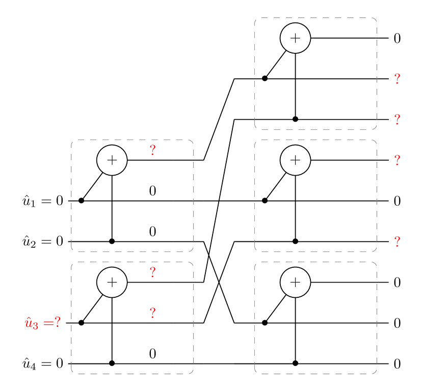
(a)

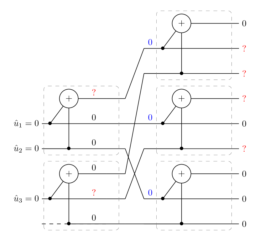
(b)

Figure 6: (a) illustrates the output of Elias’ decoding and (b) shows that $u_{3}$ indeed is correctly decoded by SC decoding for this erasure pattern. Note that the blue labeled values denote the hard-decisions propagating from left to right in SC decoding.

IV-A2 Asymptotic Performance Analysis

We consider now the asymptotic performance of SPC product codes. More specifically, we analyze the error probability of a product code sequence, defined by an ordered sequence of component code sets

$$\mathscr{C}^{{\color[rgb]{0,0,0}[m]}}=\left\{\mathcal{C}_{1},\mathcal{C}_{2},\ldots,\mathcal{C}_{m}\right\}$$

where we constrain $\left|\mathscr{C}^{{\color[rgb]{0,0,0}[m]}}\right|=m$, i.e., where the number of component codes for the $m$-th product code in the sequence is set to $m$, and the component code rates satisfy $R_{i}\leq R_{j}$ for $i<j$. We denote by $\mathcal{C}^{{\color[rgb]{0,0,0}[m]}}$ the $m$-th product code in the sequence corresponding to the set $\mathscr{C}^{{\color[rgb]{0,0,0}[m]}}$. We aim at studying the behavior of the error probability as the dimension $m$ tends to infinity when the SC decoding starts from $\mathcal{C}_{1}$ up to $\mathcal{C}_{m}$. We remark that, as $m$ changes, the component codes used to construct the product code are allowed to change, i.e., the sequence of product codes is defined by the set of component codes employed for each value of $m$. Observe that the rate of $\mathcal{C}^{{\color[rgb]{0,0,0}[m]}}$ may vanish as $m$ grows large, if the choice of the component codes forming the sets $\mathscr{C}^{{\color[rgb]{0,0,0}[m]}}$ is not performed carefully. We proceed by analyzing the limiting behavior in terms of block erasure thresholds for different product code sequences with positive rates under SC decoding. Recall that we consider $m$-dimensional systematic SPC product code constructions, where component code generator matrices $\bm{G}_{{\color[rgb]{0,0,0}1}},\dots,\bm{G}_{{\color[rgb]{0,0,0}m}}$ are obtained by removing the first rows of the kernels $\bm{\mathsf{K}}_{n_{1}},\dots,\bm{\mathsf{K}}_{n_{m}}$ of the form (15).

Definition 1.

The SC decoding block erasure threshold of a SPC product code sequence defined by the component code sets $\mathscr{C}^{[1]},\ldots,\mathscr{C}^{[m]}$ is the largest channel erasure probability $\epsilon^{\star}$ for which the block error probability $P_{\mathrm{SC}}\left(\mathcal{C}^{{\color[rgb]{0,0,0}[m]}}\right)$ converges to $0$ asymptotically in $m$ if the limit exists, i.e.,

$$\epsilon^{\star}=\sup_{\epsilon_{\mathrm{ch}}\in[0,1)}\{\epsilon_{\mathrm{ch}}:\lim_{m\rightarrow\infty}P_{\mathrm{SC}}\left(\mathcal{C}^{{\color[rgb]{0,0,0}[m]}}\right)=0\}.$$ (46)

As it is not possible to evaluate $P_{\mathrm{SC}}\left(\mathcal{C}^{{\color[rgb]{0,0,0}[m]}}\right)$ exactly, we rely on the upper bound (40) to obtain a lower bound $\epsilon^{\star}_{\mathrm{LB}}$ on the block erasure threshold in the form

$$\epsilon^{\star}_{\mathrm{LB}}=\sup_{\epsilon_{\mathrm{ch}}\in[0,1)}\{\epsilon_{\mathrm{ch}}:\lim_{m\rightarrow\infty}k\left(\mathcal{C}^{{\color[rgb]{0,0,0}[m]}}\right)\epsilon_{\mathrm{max}}\left(\mathcal{C}^{{\color[rgb]{0,0,0}[m]}}\right)=0\}$$ (47)

where the dependence of the code dimension $k$ and of the maximum information bit erasure probability $\epsilon_{\mathrm{max}}$ on the sequence of product codes has been made explicit. We provide next two examples of product code sequences, whose rates converge to a positive value. The first sequence exhibits a positive block erasure threshold (lower bound), which is however arguably far from the Shannon limit. We then analyze a product code sequence that is known to achieve the BEC capacity under bit-wise maximum a posteriori (MAP) decoding [42, 43].

Example 3 (Euler’s infinite-product representation of the sine function as an SPC product code).

Consider an SPC product code sequence with an $(a^{2}\ell^{2},a^{2}\ell^{2}-1)$ SPC component code at the $\ell$-th dimension, yielding $R_{\ell}=\left(1-(a\ell)^{-2}\right)$, with $\ell=1,\ldots,m$. The asymptotic rate is computed easily via the Euler’s infinite-product representation of the sine function, i.e.,

$$\sin\left(\frac{\pi}{a}\right)=\frac{\pi}{a}\prod_{\ell=1}^{\infty}\left(1-\frac{1}{a^{2}\ell^{2}}\right)$$

yielding an asymptotic rate $R=\frac{a}{\pi}\sin\left(\frac{\pi}{a}\right)$. Different product code sequences can be obtained for various choices of the parameter $a$. The lower bounds on the block erasure thresholds are provided in Table I for several values of $a$. The second column in Table I provides the asymptotic rate of the SPC product code sequence defined by the parameter $a$ (whose squared value is reported in the first column). The third column reports the lower bound on the block erasure threshold. The fourth column gives the Shannon limit for the given asymptotic rate, while the last one shows the fraction of the Shannon limit achieved by each construction. The thresholds achieved by the different product code sequences lie relatively far from the Shannon limit. In relative terms, the lowest-rate construction (obtained for $a^{2}=2$) achieves the largest fraction (above $1/2$) of the limit, while the efficiency of the sequences decreases as the rate grows.

TABLE I: Lower bounds on the block erasure thresholds for some SPC product code sequences based on Euler’s infinite-product representation of the sine function

$a^{2}$	$R$	$\epsilon^{\star}_{{\color[rgb]{0,0,0}\mathrm{LB}}}$	Limit, $\epsilon=1-R$	$\epsilon^{\star}_{{\color[rgb]{0,0,0}\mathrm{LB}}}/\epsilon$
$2$	$0.3582$	$0.3308$	$0.6418$	$0.5154$
$4$	$0.6366$	$0.1440$	$0.3634$	$0.3963$
$8$	$0.8067$	$0.0681$	$0.1933$	$0.3523$
$16$	$0.9003$	$0.0332$	$0.0997$	$0.3331$
$32$	$0.9494$	$0.0164$	$0.0506$	$0.3241$
$64$	$0.9745$	$0.0081$	$0.0255$	$0.3176$

Example 4 (Product of $(m,m-1)$ SPC product codes in $m$ dimensions).

We consider now the product code obtained by iterating $(m,m-1)$ SPC codes in $m$ dimensions, i.e., the resulting code is an $(m^{m},(m-1)^{m},2^{m})$ code. Hence, the rate of the $m$th product code in the sequence is

$$R\left(\mathcal{C}^{{\color[rgb]{0,0,0}[m]}}\right)=\left(1-\frac{1}{m}\right)^{m}$$

and it converges, for $m\rightarrow\infty$, to $\texttt{e}^{-1}$. As presented in [43], this product code sequence is remarkable: It is capacity-achieving over the BEC under bit-wise MAP decoding. This observation follows from results derived in [42]. Disappointingly, the block-wise erasure threshold under SC decoding turns out to be zero. This (negative) result is provided by the following theorem.

Theorem 2.

Under SC decoding, the block erasure threshold of the product code sequence defined by the component code sets $\mathscr{C}^{{\color[rgb]{0,0,0}[m]}}=\left\{\mathcal{C}_{1},\mathcal{C}_{2},\ldots,\mathcal{C}_{m}\right\}$, where $\mathcal{C}_{i}$, $i=1,\dots,m$, are $(m,m-1)$ SPC codes, is zero.

Proof.

The proof revolves around the following idea: For the product code with $(m,m-1)$ SPC component codes in $m$ dimensions over the BEC, the largest information bit erasure probability $\epsilon_{\mathrm{max}}$ under SC decoding is equal to the channel erasure probability $\epsilon_{\mathrm{ch}}\in(0,1)$, i.e., $\epsilon_{\mathrm{max}}=\epsilon_{\mathrm{ch}}$ as $m\rightarrow\infty$, which is proved below after this paragraph. Since the largest information bit erasure probability ${\color[rgb]{0,0,0}\epsilon}_{\mathrm{max}}$ is a lower bound on the block error probability under SC decoding (see (39)), we have that $\epsilon^{\star}=0$.

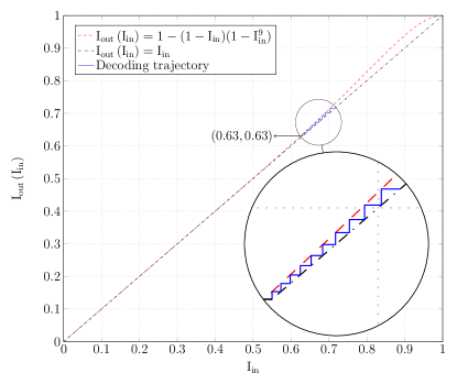
Figure 7: Decoding trajectory for the bit $u_{1}$ of the $10$-dimensional SPC product code, where the component codes are $(10,9)$ SPC codes, over the BEC$\left(0.37\right)$.

We rewrite the recursion (37), for $i=1$ and $j=1$, in mutual information as

$${\color[rgb]{0,0,0}I^{(1)}_{\bm{G}^{[m]}}}=1-\left[1-{\color[rgb]{0,0,0}I^{(1)}_{\bm{G}^{[m-1]}}}\right]\left[1-{\color[rgb]{0,0,0}\left(I^{(1)}_{\bm{G}^{[m-1]}}\right)}^{n_{m}-1}\right]$$ (48)

by noting that ${\color[rgb]{0,0,0}I^{(i)}_{\bm{G}^{[m]}}}=1-{\color[rgb]{0,0,0}\epsilon^{(i)}_{\bm{G}^{[m]}}}$ where $I^{(i)}_{\bm{G}^{[m]}}$ denotes the mutual information of the BEC with an erasure probability of $\epsilon^{(i)}_{\bm{G}^{[m]}}$ with uniform inputs. We are interested in $\mathrm{I}_{\mathrm{min}}\triangleq 1-\epsilon_{\mathrm{max}}$ for a given BEC$(\epsilon_{\mathrm{ch}})$, with $\epsilon_{\mathrm{ch}}\in[0,1)$, which can be calculated recursively via (48). This recursion is illustrated in Fig. 7 for the case $m=10$ and $\epsilon_{\mathrm{ch}}=0.37$ as an example. Note that, for the considered construction, we have $n_{\ell}=m$, $\ell=1,\dots,m$. This means that the top curve in the figure shifts down for a larger $m$, resulting in a narrower tunnel between the two curves, although the number of recursions, equal to $m$, increases. Note that it is necessary to have $\mathrm{I}_{\mathrm{min}}\rightarrow 1$, i.e., one reaches the $(1,1)$ point, with $m$ recursions in the figure for $P_{\mathrm{SC}}\rightarrow 0$. In the following, we provide an answer for the question on the dominating effect (narrower tunnel or more recursions) with increasing $m$.

The first (and single) recursion is simplified, using the RHS of (48) by setting the input $\mathrm{I}_{\mathrm{ch}}\triangleq 1-\epsilon_{\mathrm{ch}}$, as the following input-output relationship

$${\color[rgb]{0,0,0}f}(\mathrm{I}_{\mathrm{ch}}) \triangleq 1-\left(1-\mathrm{I}_{\mathrm{ch}}\right)\left(1-\mathrm{I}_{\mathrm{ch}}^{m-1}\right)$$

$$=\mathrm{I}_{\mathrm{ch}}+\mathrm{I}_{\mathrm{ch}}^{m-1}-\mathrm{I}_{\mathrm{ch}}^{m}.$$ (49)

Hence, we know that the mutual information after $m$ iterations is $\mathrm{I}_{\mathrm{min}}={\color[rgb]{0,0,0}f}^{\circ m}\left(\mathrm{I}_{\mathrm{ch}}\right)$ where ${\color[rgb]{0,0,0}f}^{\circ m}\left(\mathrm{I}_{\mathrm{ch}}\right)={\color[rgb]{0,0,0}f}\left({\color[rgb]{0,0,0}f}^{\circ m-1}\left(\mathrm{I}_{\mathrm{ch}}\right)\right)$ denotes the $m$-th iteration of function ${\color[rgb]{0,0,0}f}$ with ${\color[rgb]{0,0,0}f}^{\circ 1}\left(\mathrm{I}_{\mathrm{ch}}\right)\triangleq{\color[rgb]{0,0,0}f}\left(\mathrm{I}_{\mathrm{ch}}\right)$. We are interested in the lowest channel mutual information for which the block error rate converges to zero asymptotically in $m$, i.e.,

$$\mathrm{I}^{\star}=\inf_{\mathrm{I}_{\mathrm{ch}}\in(0,1]}\{\mathrm{I}_{\mathrm{ch}}:\lim_{m\rightarrow\infty}P_{\mathrm{SC}}\rightarrow 0\}.$$

Consider now an arbitrary $\delta>0$. For any positive $\gamma<1$, there exists a sufficiently large $m$ such that $m\gamma^{m-2}\leq\delta$. Then, for any non-negative $\mathrm{I}\leq\gamma$, we write

$${\color[rgb]{0,0,0}f}(\mathrm{I}) =\mathrm{I}+\mathrm{I}^{m-1}-\mathrm{I}^{m}$$ (50)

$$\leq\mathrm{I}\left(1+\mathrm{I}^{m-2}\right)$$ (51)

$$\leq\mathrm{I}\left(1+\frac{\delta}{m}\right)$$ (52)

where (51) follows from the fact that $\mathrm{I}\geq 0$ and (52) from the fact that $\mathrm{I}\leq\gamma$, which, combined with $m\gamma^{m-2}\leq\delta$, leads to $\mathrm{I}^{m-2}\leq\frac{\delta}{m}$. For any initial $\mathrm{I}_{\mathrm{ch}}\leq\texttt{e}^{-\delta}\gamma$ and any $m^{\prime}\leq m$, we have

$${\color[rgb]{0,0,0}f}^{\circ m^{\prime}}(\mathrm{I}_{\mathrm{ch}})\leq\texttt{e}^{-\delta}\gamma\left(1+\frac{\delta}{m}\right)^{m^{\prime}}\leq\gamma$$ (53)

which makes sure that the condition $\mathrm{I}\leq\gamma$ for (52) is not violated with $m^{\prime}$ iterations. Therefore, for any positive $\gamma<1$, any $\delta>0$ and any $\mathrm{I}_{\mathrm{ch}}\leq\texttt{e}^{-\delta}\gamma$, we write

$$\lim_{m\rightarrow\infty}{\color[rgb]{0,0,0}f}^{\circ m}(\mathrm{I}_{\mathrm{ch}})\leq\mathrm{I}_{\mathrm{ch}}\texttt{e}^{\delta}.$$ (54)

The result follows by choosing $\delta$ arbitrarily small and $\gamma$ arbitrarily close to $1$. $\blacksquare$

IV-B Analysis over Binary Memoryless Symmetric Channels

It is well-known that the block error probability of polar codes under SC decoding can be analyzed using density evolution, when the transmission takes place over a BMS channel[41]. In the following, the same method is used to provide a tight upper bound on the block error probability of SPC product codes over BMS channels.

Due to the channel symmetry and the linearity of the codes, we assume that the all-zero codeword is transmitted. We write $L^{(i)}_{{\color[rgb]{0,0,0}\bm{G}^{[m]}}}(\bm{y},\bm{0})$ to denote the the log-likelihood ratio for $u_{i}$ based on (21) where all the previous bit-values are provided as zeros to the decoder, i.e.,

$$L^{(i)}_{{\color[rgb]{0,0,0}\bm{G}^{[m]}}}(\bm{y},\bm{0})\triangleq\log\frac{\mathrm{W}^{(i)}_{{\color[rgb]{0,0,0}\bm{G}^{[m]}}}(\bm{y},U_{1}^{i-1}=\bm{0}|U_{i}=0)}{\mathrm{W}^{(i)}_{{\color[rgb]{0,0,0}\bm{G}^{[m]}}}(\bm{y},U_{1}^{i-1}=\bm{0}|U_{i}=1)}.$$

Accordingly, we use $l^{(i)}_{{\color[rgb]{0,0,0}\bm{G}^{[m]}}}$ to denote the probability density function (p.d.f.) of the RV $L^{(i)}_{{\color[rgb]{0,0,0}\bm{G}^{[m]}}}(Y_{1}^{n},\bm{0})$. Extending the equations (36) and (37) to general BMS channels, the densities can be computed recursively as

$$l^{(i)}_{{\color[rgb]{0,0,0}\bm{G}^{[m]}}}=l^{(j+1)}_{{\color[rgb]{0,0,0}\bm{G}^{[m-1]}}}\varoast(l^{(j+1)}_{{\color[rgb]{0,0,0}\bm{G}^{[m-1]}}})^{\boxast(n_{m}-t)}$$ (55)

with $j=\lfloor\nicefrac{{(i-1)}}{{k_{m}}}\rfloor$ and $t\triangleq[(i-1)\!\!\mod k_{m}]+1$ where $\varoast$ denotes the variable node convolution and $(l^{(j+1)}_{{\color[rgb]{0,0,0}\bm{G}^{[m-1]}}})^{\boxast(a)}$ the $a$-fold check node convolution with $(l^{(j+1)}_{{\color[rgb]{0,0,0}\bm{G}^{[m-1]}}})^{\boxast(1)}\triangleq l^{(j+1)}_{{\color[rgb]{0,0,0}\bm{G}^{[m-1]}}}$ as defined in [44, Ch. 4]. Then, the RHS of (27) can be computed via $l^{(i)}_{{\color[rgb]{0,0,0}\bm{G}^{[m]}}}$ with $i=1,\dots,k$, i.e., as

$$\sum_{i=1}^{k}\lim\limits_{z\rightarrow 0}\left(\int_{-\infty}^{-z}l^{(i)}_{{\color[rgb]{0,0,0}\bm{G}^{[m]}}}(x)dx+\frac{1}{2}\int_{-z}^{+z}l^{(i)}_{{\color[rgb]{0,0,0}\bm{G}^{[m]}}}(x)dx\right).$$ (56)

The computation of (55) and (56) can be carried out, for instance, via quantized density evolution [45], yielding an accurate estimate of the RHS of (27).

In Fig. 8, we provide simulation results for the $(125,64)$ SPC product code over the B-AWGN channel. The results are provided in terms of BLER vs. signal-to-noise ratio (SNR), where the SNR is expressed as $E_{b}/N_{0}$ ($E_{b}$ is here the energy per information bit and $N_{0}$ the single-sided noise power spectral density). The SC decoding performance is compared to the performance under Elias’ and BP decoding. While it was only proven for the case of BEC in Theorem 42, the results illustrate that the SC decoding outperforms Elias’ decoding also over the B-AWGN channel for the simulated code. BP decoding with a maximum number of iterations set to $100$ outperforms the SC decoding significantly, which motivates us to introduce SCL decoding in the next section. The tight upper bound on the SC decoding, computed via (56), is also provided.

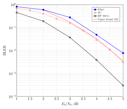
Figure 8: BLER vs. SNR over the B-AWGN channel for a $(125,64)$ product code under SC decoding, compared to Elias’ decoding as well as a BP decoding with $100$ iterations.

V Successive Cancellation List Decoding of Single Parity-Check Product Codes

While the asymptotic analysis provided in Section IV-A2 provides some insights on the SPC product codes constructed over a large number of dimensions (yielding very large block lengths), we are ultimately interested in the performance of product codes in the practical setting where the number of dimensions is small, and the block length is moderate (or small). Like polar codes, SC decoding of SPC product codes performs poorly in this regime, e.g., see Fig. 8. Hence, following the footsteps of [25], we investigate the error probability of SPC product codes under SCL decoding. The SC decoder decides on the value of $u_{i}$, $1\leq i\leq k$, after computing the corresponding likelihood. The SCL decoder does not make a final decision on the bit value $u_{i}$ immediately. Instead, it considers both options (i.e., $\hat{u}_{i}=0$ and $\hat{u}_{i}=1$) and runs several instances of the SC decoder in parallel. Each SC decoder corresponds to a decoding path, defined by a given different hypothesis on $i-1$ preceding information bits, namely $\hat{u}_{1}^{i-1}$, $1<i<k$, at decoding stage $i$. After computing the likelihood for $u_{i}$, a path is split into two new paths, that share the same decisions $\hat{u}_{1}^{i-1}$ for the preceding $i-1$ bits. But these new paths consider different decisions for $\hat{u}_{i}$ (i.e., $\hat{u}_{i}=0$ and $\hat{u}_{i}=1$), respectively, which doubles the number of paths at each decoding stage. In order to avoid an excessive growth in the number of paths, a maximum list size $L$ is imposed. The SCL decoder discards the paths except for the most likely paths, according to metrics computed via (21), whenever their number exceeds the list size $L$. After $k$ steps, among the surviving $L$ candidates, the SCL decoder chooses as the final decision the candidate path maximizing the likelihood, yielding a decision $\hat{\bm{u}}$. Obviously, the block error rate decreases with an increasing $L$ at the expense of a higher complexity.

Remark 3.

For short- and moderate-length polar codes, it was shown in [25] that close-to-ML performance can be attained with a sufficiently large (yet, manageable) list size. This was demonstrated by computing a numerical lower bound on the ML decoding error probability via Monte Carlo simulation, where the correct codeword is introduced artificially in the final list, prior to the final decision. If, for a specific list size $L$, the simulated error probability is close to the numerical ML decoding lower bound, then increasing the list size $L$ would not yield any performance improvement. The same principle applies to SCL decoding of SPC product codes.

Owing to this observation, we first study the performance of SPC product codes under ML decoding, by developing a weight enumerator analysis. Similarly, inspired by the concatenated polar code construction of [25], we also study the performance of a concatenation of a high-rate outer code with an inner SPC product code under ML decoding. For both cases, the analysis is complemented by the SCL decoding simulations. We will see that (for some short product codes) the ML decoding performance is indeed attainable by SCL decoding with small list sizes, e.g., $L\leq 8$, while moderate list sizes, e.g., $128\leq L\leq 1024$, are required when SPC product codes are concatenated with an outer code.

V-A Finite-length Performance Analysis via Weight Distribution of SPC Product Codes

Computing the weight enumerator of SPC product codes for small constructions is feasible using the method presented in [14]. First, we provide an alternative derivation to the WEF of a $2$-dimensional product code $\mathcal{C}$ with systematic arbitrary binary linear component code $\mathcal{C}_{1}$ and systematic $(\nu,\nu-1)$ SPC code $\mathcal{S}_{\nu}$ as the second component code.

Theorem 3.

Let $\mathcal{C}_{1}$ and $\mathcal{S}_{\nu}$ be an arbitrary $(n_{1},k_{1})$ systematic code with a generator matrix $\bm{G}$ and a length-$\nu$ systematic SPC code, respectively. Then, the WEF of the product code $\mathcal{C}$ with component codes $\mathcal{C}_{1}$ and $\mathcal{S}_{\nu}$ is

$$A_{\mathcal{C}}(z)=2^{-k_{\scaleto{1}{3pt}}}\sum_{\bm{v}\in\{0,1\}^{k_{\scaleto{1}{3pt}}}}\left(\sum_{\bm{u}\in\{0,1\}^{k_{\scaleto{1}{3pt}}}}(-1)^{\bm{u}\cdot\bm{v}^{\mathrm{T}}}z^{w_{\scaleto{\mathrm{H}}{3pt}}\left(\bm{u}{\color[rgb]{0,0,0}\bm{G}}\right)}\right)^{\nu}.$$ (57)

Proof.

Let $f(\bm{Z})=\prod_{i=1}^{\nu}f_{i}(z_{i,1},\ldots,z_{i,n})$ be a multinomial in the variables $\bm{Z}=\{z_{i,j}\}$, $1\leq i\leq\nu$, $1\leq j\leq{\color[rgb]{0,0,0}n}$, where each factor $f_{i}$ is a multinomial only in the variables $z_{i,1},\ldots,z_{i,n}$. Assume further that each variable $z_{i,j}$ appears with exponent either $0$ or $1$ in the multinomial $f_{i}(z_{i,1},\ldots,z_{i,n})$, and, hence, in $f(\bm{Z})$. Suppose now that we wish to remove from $f(\bm{Z})$ all the terms in the form

$$\prod_{i\in\mathcal{T}}z_{i,j}$$ (58)

where $|\mathcal{T}|$ is odd. The remaining terms can be obtained by computing

$$\frac{1}{2}\sum_{y\in\{+1,-1\}}\prod_{i=1}^{\nu}f_{i}(z_{i,1},\ldots,z_{i,j-1},yz_{i,j},z_{i,j+1},\ldots,z_{i,n}).$$ (59)

Similarly, to remove all the terms in the form

$$\prod_{i\in\mathcal{T}_{j}}z_{i,j},\quad j\in[n]$$ (60)

where $|\mathcal{T}_{j}|$ is odd, it is sufficient to evaluate

$$2^{-n}\sum_{\bm{y}\in\{+1,-1\}^{n}}\prod_{i=1}^{\nu}f_{i}(y_{1}z_{i,1},\ldots,y_{n}z_{i,n}).$$ (61)

Consider first a product code composed of $\nu\times n_{1}$ arrays whose rows and columns are codewords of $\mathcal{C}_{1}$ and a trivial rate-$1$ code $\mathcal{I}$ with a generator matrix $\bm{I}_{\nu}$, respectively. Then, the complete WEF $A_{\mathcal{C}_{1}\otimes\mathcal{I}}(\bm{Z})$ of the product code uses the dummy variables $\bm{Z}=\{z_{i,j}\}$, $1\leq i\leq\nu$, $1\leq j\leq n_{1}$, to track bits by their $(i,j)$ coordinate in the codeword. This is obtained simply by the multiplication of the complete WEFs for the codes corresponding to each row $i$, i.e., we have

$$A_{\mathcal{C}_{1}\otimes\mathcal{I}}(\bm{Z})=\prod_{i=1}^{\nu}A_{\mathcal{C}_{\scaleto{1}{3pt}}}(z_{i,1},\ldots,z_{i,n_{\scaleto{1}{3pt}}}).$$ (62)

Recall now that the codewords of $\mathcal{C}$ are $\nu\times n_{1}$ arrays whose rows and columns are codewords of $\mathcal{C}_{1}$ and $\mathcal{S}_{\nu}$, respectively. Then, the complete WEF $A_{\mathcal{C}}(\bm{Z})$ of the product code $\mathcal{C}$ is derived from $A_{\mathcal{C}_{1}\otimes\mathcal{I}}(\bm{Z})$ by imposing that each column word has an even weight, i.e., we have

$$\!\!\!\!\!\!\!\!A_{\mathcal{C}}(\bm{Z})=2^{-n_{\scaleto{1}{3pt}}}\sum_{\bm{y}\in\{+1,-1\}^{n_{\scaleto{1}{3pt}}}}\prod_{i=1}^{\nu}A_{\mathcal{C}_{\scaleto{1}{3pt}}}(y_{1}z_{i,1},\dots,y_{n_{\scaleto{1}{3pt}}}z_{i,n_{\scaleto{1}{3pt}}}).$$ (63)

Then, the WEF of the product code $\mathcal{C}$ is obtained by setting $z_{i,j}=z$, yielding

$$A_{\mathcal{C}}(z)=2^{-n_{\scaleto{1}{3pt}}}\sum_{\bm{y}\in\{1,-1\}^{n_{\scaleto{1}{3pt}}}}\left(A_{\mathcal{C}_{\scaleto{1}{3pt}}}(y_{1}z,\dots,y_{n_{\scaleto{1}{3pt}}}z)\right)^{\nu}$$ (64)

$$=2^{-n_{\scaleto{1}{3pt}}}\sum_{\bm{y}\in\{1,-1\}^{n_{\scaleto{1}{3pt}}}}\left(\sum_{\bm{x}\in\mathcal{C}_{1}}z^{w_{\scaleto{\mathrm{H}}{3pt}}(\bm{x})}\prod_{i^{\prime}=1}^{n_{1}}y_{i^{\prime}}^{x_{i^{\prime}}}\right)^{\nu}$$ (65)

$$=2^{-n_{\scaleto{1}{3pt}}}\sum_{\bm{y}\in\{0,1\}^{n_{\scaleto{1}{3pt}}}}\left(\sum_{\bm{x}\in\mathcal{C}_{1}}z^{w_{\scaleto{\mathrm{H}}{3pt}}\left(\bm{x}\right)}(-1)^{\bm{x}\cdot\bm{y}^{\mathrm{T}}}\right)^{\nu}$$ (66)

$$=2^{-n_{\scaleto{1}{3pt}}}\sum_{\bm{y}\in\{0,1\}^{n_{\scaleto{1}{3pt}}}}\left(\sum_{\bm{u}\in\{0,1\}^{k_{\scaleto{1}{3pt}}}}z^{w_{\scaleto{\mathrm{H}}{3pt}}\left(\bm{u}\bm{G}\right)}(-1)^{\bm{u}\bm{G}\bm{y}^{\mathrm{T}}}\right)^{\nu}$$ (67)

$$=2^{-n_{\scaleto{1}{3pt}}}\sum_{\bm{y}\in\{0,1\}^{n_{\scaleto{1}{3pt}}}}\left(\sum_{\bm{u}\in\{0,1\}^{k_{\scaleto{1}{3pt}}}}z^{w_{\scaleto{\mathrm{H}}{3pt}}\left(\bm{u}\bm{G}\right)}(-1)^{\bm{u}\bm{G}\tilde{\bm{H}}\bm{y}^{\mathrm{T}}}\right)^{\nu}$$ (68)

$$=2^{-n_{\scaleto{1}{3pt}}}\!\sum_{y_{1}^{n_{\scaleto{1}{3pt}}-k_{\scaleto{1}{3pt}}}}\!\sum_{\bm{v}\in\{0,1\}^{k_{\scaleto{1}{3pt}}}}\!\!\left(\sum_{\bm{u}\in\{0,1\}^{k_{\scaleto{1}{3pt}}}}\!\!z^{w_{\scaleto{\mathrm{H}}{3pt}}\left(\bm{u}\bm{G}\right)}(-1)^{\bm{u}\bm{G}\bar{\bm{H}}^{\mathrm{T}}\bm{v}^{\mathrm{T}}}\!\right)^{\nu}$$ (69)

with $\tilde{\bm{H}}\triangleq\left[\bm{H}^{\mathrm{T}},\bar{\bm{H}}^{\mathrm{T}}\right]$ where $\bm{H}$ and $\bar{\bm{H}}$ are the parity-check matrix of $\mathcal{C}_{1}$ and a complementary matrix such that $\tilde{\bm{H}}$ is non-singular, respectively, and $\bm{v}\triangleq y_{n_{\scaleto{1}{3pt}}-k_{\scaleto{1}{3pt}}+1}^{n_{\scaleto{1}{3pt}}}$. Note that (65) follows from (5) by noting that $(y_{1}z,\ldots,y_{n_{\scaleto{1}{3pt}}}z)^{\bm{x}}=z^{w_{\scaleto{\mathrm{H}}{3pt}}(\bm{x})}\bm{y}^{\bm{x}}$, (66) from re-defining the dummy vector $\bm{y}$, (67) from $\bm{x}=\bm{u}\bm{G}$ and performing the summation over $\bm{u}\in\{0,1\}^{k_{\scaleto{1}{3pt}}}$ instead of $\bm{x}\in\mathcal{C}_{\scaleto{1}{3pt}}$, (68) from the nonsingularity of $\tilde{\bm{H}}$ and the summation being over all possible $\bm{y}\in\{0,1\}^{n_{\scaleto{1}{3pt}}}$, and (69) from dividing the outer summation into two parts, namely over $y_{1}^{n_{\scaleto{1}{3pt}}-k_{\scaleto{1}{3pt}}}\in\{0,1\}^{n_{\scaleto{1}{3pt}}-k_{\scaleto{1}{3pt}}}$ and $\bm{v}\in\{0,1\}^{k_{\scaleto{1}{3pt}}}$, and the fact that the product $\bm{G}\bm{H}^{\mathrm{T}}$ results in the all-zero matrix. Finally, (57) follows from the fact that the outer summation can be removed by multiplying the remaining term by $2^{n_{\scaleto{1}{3pt}}-k_{\scaleto{1}{3pt}}}$ and the fact that the product $\bm{G}\bar{\bm{H}}^{\mathrm{T}}$ is non-singular. $\blacksquare$

Thanks to Theorem 3, one can compute the WEF of short and moderate-length SPC product codes iteratively, by simply choosing one component code to be a SPC product code $\mathcal{C}_{1}$ and the other one to be a SPC code $\mathcal{S}_{\nu}$. Given the weight enumerator of a product code, upper bounds on the ML decoding error probability can be obtained. As an example, a tight bound on the block error probability over the B-AWGN channel is provided by Poltyrev’s TSB [26]. Another example of a tight bound on the block error probability of a code based on its weight enumerator is Di’s union bound over the BEC [30, Lemma B.2]. We refer the interested reader to [46] for an extensive survey on performance bounds under ML decoding.

Next, we provide simulation results for the $3$-dimensional $(125,64)$ SPC product code under ML decoding implemented over the BEC via SCL decoding with $L=\infty$. The results are provided in Fig. 9. As reference, simulation results for a $(125,64)$ punctured polar code [47] are also provided, where the polar code design follows the guidelines of the 5G standard [48]. The polar code slightly outperforms the considered SPC product code. Note that Di’s union bound tightly approaches the performance of the SPC product code.

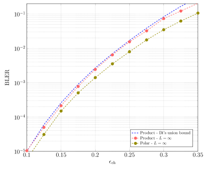
Figure 9: BLER vs. $\epsilon_{\mathrm{ch}}$ over the BEC for the $(125,64)$ product code under ML decoding, implemented via SCL decoding with $L=\infty$, compared to a $(125,64)$ punctured polar code.

The same $(125,64)$ SPC product code is also simulated over the B-AWGN channel under SCL decoding with various list sizes. The results are given in Fig. 10. The TSB is also provided, thanks to the weight enumerator analysis. Remarkably, SCL decoding with $L=4$ is sufficient to operate very close to the TSB and to outperform BP decoding. With $L=8$, the SCL decoder tightly approaches the ML lower bound, which is not the case for BP decoding. The RCU [27, Thm. 16] and the metaconverse (MC) [27, Thm. 26] bounds, are here plotted as reference. The gap to the RCU bound reaches to $1.7$ dB at BLER of $10^{-3}$.

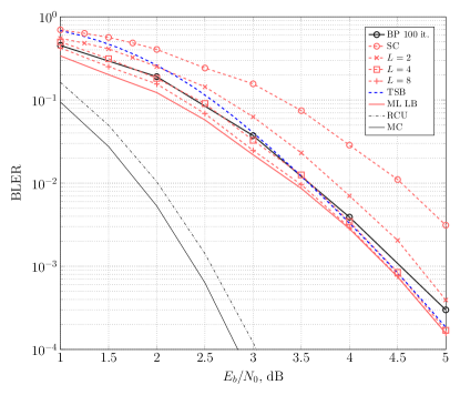
Figure 10: BLER vs. SNR under SCL decoding for the $(125,64)$ product code with various list sizes, compared to a BP decoding with $100$ iterations.

The performance of SPC product codes is compared to that of the $(125,64)$ polar code in Fig. 11. When $L=4$ is considered, the performance of polar code tightly matches its ML lower bound and outperforms the SPC product code by around $0.3$ dB at BLER of $10^{-3}$. The gap between their ML performance is around $0.25$ dB. Note that the polar code requires a smaller list size to approach its ML performance.

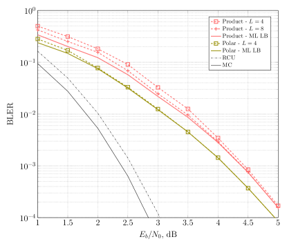
Figure 11: BLER vs. SNR over the B-AWGN channel for the $(125,64)$ product code under SCL decoding with various list sizes, compared to a $(125,64)$ punctured polar code.

V-B Finite-length Performance Analysis via Average Weight Distribution of Concatenated Ensembles

Following [25], SPC product codes are concatenated with a high-rate outer code to improve the distance profile, aiming at an improved performance under SCL (and ML) decoding. At the receiver, an SCL decoder with list size $L$ is employed for the inner code. The outer code is used to test the $L$ codewords in the final list. Among those satisfying the outer code constraints, the most likely one is chosen as the final decision. Our goal is to analyze the ML decoding performance of the concatenated code, since for short and moderate blocklengths close-to-ML performance may be practically attained via SCL decoding by choosing a sufficiently large list. To analyze the ML decoding performance of such a concatenation, we first derive the weight enumerator of product codes in concatenation with an outer code. The weight enumerators will then be used to derive well-known tight upper bounds on the ML decoding error probability as before. A reason to analyze such concatenation lies (besides in the expected performance improvement) in the fact that actual schemes employing product codes may make use of an error detection code to protect the product code information message (this is the case, for instance, of the IEEE 802.16 standard [28]). One may hence consider sacrificing (part of) the error detection capability introduced by the outer error detection code for a larger coding gain [20].

Consider the concatenation of an $(n_{\mathsf{i}},k_{\mathsf{i}})$ inner product code $\mathcal{C}_{\mathsf{i}}$ with an $(n_{\mathsf{o}},k_{\mathsf{o}})$ high-rate outer code $\mathcal{C}_{\mathsf{o}}$ with $k_{\mathsf{i}}=n_{\mathsf{o}}$. The generator matrices of $\mathcal{C}_{\mathsf{i}}$ and $\mathcal{C}_{\mathsf{o}}$ are $\bm{G}_{\mathsf{i}}$ and $\bm{G}_{\mathsf{o}}$, respectively.

Definition 2 (Concatenated Ensemble).

The (serially) concateneted ensemble $\mathscr{C}\left(\mathcal{C}_{\mathsf{o}},\mathcal{C}_{\mathsf{i}}\right)$ is the set of all codes with generator matrix of the form

$$\bm{G}=\bm{G}_{\mathsf{o}}\bm{\Pi}\bm{G}_{\mathsf{i}}$$

where $\bm{\Pi}$ is an $n_{\mathsf{o}}\times n_{\mathsf{o}}$ permutation matrix.

Assume that the outer code weight enumerator $A^{\mathsf{o}}_{j}$ and the input-output weight enumerator of the inner product code $A^{\mathrm{IO},\mathsf{i}}_{j,w}$ are known. We are interested in the weight enumerator of the concatenated code for a given permutation matrix $\bm{\Pi}$ (e.g., $\bm{\Pi}=\bm{I}_{n_{\mathsf{o}}}$), which interleaves the output of the outer encoder. Given an interleaver, this requires the enumeration of all possible input vectors of length $k_{\mathsf{o}}$, which is not possible in practice. For this reason, the impact of the outer code is typically analyzed in a concatenated ensemble setting by assuming that the interleaver is distributed uniformly over all possible ${n_{\text{out}}\choose i}$ permutations[49]. Then, the average weight enumerator of the ensemble is derived as

$$\bar{A}_{w}=\sum_{j=0}^{n_{\text{out}}}\frac{A_{j}^{\mathsf{o}}\cdot A_{j,w}^{\mathrm{IO},\mathsf{i}}}{{n_{\mathsf{o}}\choose j}}$$ (70)

where $\bar{A}_{w}$ is the average multiplicity of codewords ${\color[rgb]{0,0,0}\bm{x}}$ with $w_{\mathrm{H}}({\color[rgb]{0,0,0}\bm{x}})=w$. The computation of (70) requires the knowledge of the input-output weight enumerator of the inner SPC product code. Therefore, we extend the result of Theorem 3 to the derivation of the IOWEF.

Theorem 4.

Let $\mathcal{C}_{1}$ and $\mathcal{S}_{\nu}$ be an arbitrary $(n_{1},k_{1})$ systematic code with a generator matrix ${\color[rgb]{0,0,0}\bm{G}}$ and a systematic SPC code, respectively. Then, the IOWEF of the product code $\mathcal{C}$ with component codes $\mathcal{C}_{1}$ and $\mathcal{S}_{\nu}$ is

$$A_{\mathcal{C}}^{\mathrm{IO}}(x,z)\!=\!2^{-k_{\scaleto{1}{3pt}}}\!\sum_{\bm{v}\in\{0,1\}^{k_{\scaleto{1}{3pt}}}}\!\! \left(\sum_{\bm{u}\in\{0,1\}^{k_{\scaleto{1}{3pt}}}}\!\!(-1)^{\bm{u}\cdot\bm{v}^{\mathrm{T}}}x^{w_{\scaleto{\mathrm{H}}{3pt}}\left(\bm{u}\right)}z^{w_{\scaleto{\mathrm{H}}{3pt}}\left(\bm{u}{\color[rgb]{0,0,0}\bm{G}}\right)}\!\right)^{\nu-1}$$ (71)

$$\qquad\left(\sum_{\bm{u}\in\{0,1\}^{k_{\scaleto{1}{3pt}}}}(-1)^{\bm{u}\cdot\bm{v}^{\mathrm{T}}}z^{w_{\scaleto{\mathrm{H}}{3pt}}\left(\bm{u}{\color[rgb]{0,0,0}\bm{G}}\right)}\right).$$ (72)

Proof.

Recall (63) and assume, without loss of generality, that the component code generator matrices are of the form $[\bm{I}_{k_{i}}|\bm{P}_{i}]$. In this case, we set $z_{i,j}=xz$, for $1\leq i\leq k_{1}$ and $1\leq j\leq k_{2}=\nu-1$, and $z_{i,j}=z$, otherwise, to obtain

$$A_{\mathcal{C}}(x,z)=2^{-n_{\scaleto{1}{3pt}}}\sum_{\bm{y}\in\{1,-1\}^{n_{\scaleto{1}{3pt}}}} \left(\sum_{\bm{u}\in\{0,1\}^{k_{\scaleto{1}{3pt}}}}x^{w_{\scaleto{\mathrm{H}}{3pt}}\left(\bm{u}\right)}z^{w_{\scaleto{\mathrm{H}}{3pt}}\left({\color[rgb]{0,0,0}\bm{u}\bm{G}}\right)}{\color[rgb]{0,0,0}\bm{y}^{\bm{u}\bm{G}}}\right)^{\nu-1}$$ (73)

$$\qquad\left(\sum_{\bm{u}\in\{0,1\}^{k_{\scaleto{1}{3pt}}}}z^{w_{\scaleto{\mathrm{H}}{3pt}}\left({\color[rgb]{0,0,0}\bm{u}\bm{G}}\right)}{\color[rgb]{0,0,0}\bm{y}^{\bm{u}\bm{G}}}\right)$$ (74)

where the result follows by applying the similar steps in the proof of Theorem 3. $\blacksquare$

Similar to the WEF, one can compute the IOWEF of short and moderate-length SPC product codes iteratively, by choosing one component code to be a SPC product code $\mathcal{C}_{1}$ and the other one to be a SPC code $\mathcal{S}_{\nu}$. Given the average weight enumerator of a concatenated ensemble, upper bounds on the ML decoding error probability can be obtained as in Section V-A.

Fig. 12 shows the performance of concatenating the $(125,64)$ product code with a $8$-bit outer CRC code with generator polynomial $g(x)=x^{8}+x^{6}+x^{5}+x^{4}+x^{2}+x+1$, where the interleaver between the codes is the trivial one defined by an identity matrix. This concatenation leads to a $(125,56)$ code. Since the code distance properties are improved (observed directly via the TSB on the average performance of the code ensemble), the performance improvement under ML decoding is expected to be significant. The CRC polynomial is selected as the one which provides the best TSB, obtained for the average weight enumerator of a concatenated ensemble with the uniform interleaver assumption [49]. The gain achieved by SCL decoding is remarkably large, operating below the TSB. At a BLER of $10^{-2}$, SCL decoding of the concatenated code achieves gains up to $1.25$ dB over the original product code, reaching up to $1.5$ dB at a BLER $\approx 10^{-4}$. The gap to the RCU bound is approximately $0.7$ dB at a BLER of $10^{-4}$ and less for higher BLERs, providing a competitive performance for similar parameters[39]. For example, the performance of a $(128,64)$ 5G-NR LDPC code (base graph 2, see [39]) is reported. The code has been decoded with the BP algorithm by setting the maximum number of iterations to $100$. The concatenation of the outer CRC code with the inner SPC product code yields a remarkable gain of $\approx 0.6$ dB with respect to the 5G-NR LDPC code (it shall be noted, however, that the concatenated SPC code possesses a slightly lower code rate). Note that it is not always possible to attain a performance close to the ML performance of concatenated codes using BP decoding[20, 50]. In that sense, SCL decoding provides a low-complexity solution to approach the ML performance of the concatenated SPC product code scheme. As another reference, a (125, 56) CRC-concatenated polar code is constructed by using the $(125,64)$ polar code with an $8$-bit outer CRC code optimized using the guidelines of [51], which takes into account the exact code concatenation under SCL decoding rather than an ensemble performance. The generator polynomial of the CRC code is $g(x)=x^{8}+x^{7}+x^{6}+x^{5}+1$. The gap between the ML performance of two codes is less than $0.5$ dB in the considered regime. A careful optimization of the interleaver of the CRC-concatenated SPC product code might provide further gains as for polar codes[52], but it is not in the scope of this work.

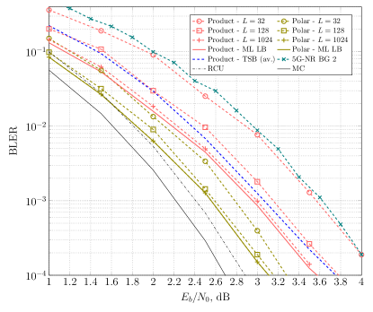
Figure 12: BLER vs. SNR over the B-AWGN channel for a $(125,64)$ product code concatenated with a $(64,56)$ CRC code under SCL decoding with various list sizes. The performance is compared to the one of a $(125,56)$ CRC-concatenated polar code with various list sizes, where the generator polynomial of the outer code is optimized for SCL decoding[51], and the one of the $(128,64)$ 5G-NR LDPC code (base graph 2, see [39]) under BP decoding where the maximum number of iterations is set to $100$.

VI Conclusions

Successive cancellation (SC) decoding was introduced for the class of product codes obtained by iterating single parity-check (SPC) codes, namely SPC product codes. As a byproduct, the relations between SPC product and multi-kernel polar codes were studied, which enables us to use tools of the latter. SPC product codes have been, then, analyzed under SC decoding over the binary memoryless symmetric channels, in particular, over the binary-input additive white Gaussian (B-AWGN) channel and the binary erasure channel (BEC).

Successive cancellation list (SCL) decoding has been described for SPC product codes as well, which outperforms belief propagation (BP) decoding even with a considerably small list sizes, e.g., $L=4$, for the demonstrated example over the B-AWGN channel. Larger gains are attained by concatenating an inner SPC product code with a high-rate outer code. The maximum-likelihood performance (with an outer code) was analyzed via (average) distance spectrum by developing an efficient method to compute the (input-output) weight enumerator of short SPC product codes, which is shown to be achieved via SCL decoding with moderate list sizes for the considered example.

While the asymptotic analysis over the BEC under SC decoding has shown, for some specific product code sequences, a considerable gap to channel capacity, finite-length results on SPC product codes show that they are well-suited for SC and SCL decoding, with performance gains over BP decoding that are especially visible when an outer error detection code is used in combination with the list decoder.

References

- [1] M. C. Coşkun, G. Liva, A. Graell i Amat, and M. Lentmaier, “Successive cancellation decoding of single parity-check product codes,” in Proc. of IEEE Int. Symp. on Inf. Theory, Aachen, Jun. 2017, pp. 1758–1762.
- [2] P. Elias, “Error-free coding,” IRE Trans. Inf. Theory, vol. PGIT-4, pp. 29–37, Sep. 1954.
- [3] C. Berrou, A. Glavieux, and P. Thitimajshima, “Near Shannon limit error-correcting coding and decoding: Turbo-codes. 1,” in IEEE Int. Conf. Commun. (ICC), vol. 2, May 1993, pp. 1064–1070.
- [4] R. M. Pyndiah, “Near-optimum decoding of product codes: block turbo codes,” IEEE Trans. Commun., vol. 46, no. 8, pp. 1003–1010, Aug. 1998.
- [5] R. Tanner, “A recursive approach to low complexity codes,” IEEE Trans. Inf. Theory, vol. 27, no. 5, pp. 533–547, Sep. 1981.
- [6] J. Li, K. R. Narayanan, and C. N. Georghiades, “Product accumulate codes: a class of codes with near-capacity performance and low decoding complexity,” IEEE Trans. Inf. Theory, vol. 50, no. 1, pp. 31–46, Jan. 2004.
- [7] A. J. Feltström, D. Truhachev, M. Lentmaier, and K. S. Zigangirov, “Braided block codes,” IEEE Trans. Inf. Theory, vol. 55, no. 6, pp. 2640–2658, Jun. 2009.
- [8] H. D. Pfister, S. K. Emmadi, and K. Narayanan, “Symmetric product codes,” in Proc. Information Theory and Applications Workshop (ITA), Feb. 2015, pp. 282–290.
- [9] C. Berrou, R. Pyndiah, P. Adde, C. Douillard, and R. L. Bidan, “An overview of turbo codes and their applications,” in Proc. European Conference on Wireless Technology, Oct. 2005, pp. 1–9.
- [10] C. Häger, H. D. Pfister, A. Graell i Amat, and F. Brännström, “Density evolution for deterministic generalized product codes on the binary erasure channel at high rates,” IEEE Trans. Inf. Theory, vol. 63, no. 7, pp. 4357–4378, Jul. 2017.
- [11] N. Abramson, “Cascade decoding of cyclic product codes,” IEEE Trans. Commun. Tech., vol. 16, no. 3, pp. 398–402, Jun. 1968.
- [12] X. Tang and R. Koetter, “Performance of iterative algebraic decoding of codes defined on graphs: An initial investigation,” in IEEE Inf. Theory Workshop (ITW), Sep. 2007, pp. 254–259.
- [13] C. Häger and H. D. Pfister, “Approaching miscorrection-free performance of product codes with anchor decoding,” IEEE Trans. Commun., vol. 66, no. 7, pp. 2797–2808, Jul. 2018.
- [14] G. Caire, G. Taricco, and G. Battail, “Weight distribution and performance of the iterated product of single-parity-check codes,” in IEEE GLOBECOM, Nov. 1994, pp. 206–211.
- [15] D. M. Rankin and T. A. Gulliver, “Single parity check product codes,” IEEE Trans. Commun., vol. 49, no. 8, pp. 1354–1362, Aug. 2001.
- [16] D. M. Rankin, T. A. Gulliver, and D. P. Taylor, “Asymptotic performance of single parity-check product codes,” IEEE Trans. Inf. Theory, vol. 49, no. 9, pp. 2230–2235, Sep. 2003.
- [17] P. Trifonov and P. Semenov, “Generalized concatenated codes based on polar codes,” in IEEE Int. Symp. Wireless Commun. Syst, Nov 2011, pp. 442–446.
- [18] E. Arıkan, “Channel polarization: A method for constructing capacity-achieving codes for symmetric binary-input memoryless channels,” IEEE Trans. Inf. Theory, vol. 55, no. 7, pp. 3051–3073, Jul. 2009.
- [19] N. Stolte, “Rekursive Codes mit der Plotkin-Konstruktion und ihre Decodierung,” Ph.D. dissertation, TU Darmstadt, 2002.
- [20] M. C. Coşkun, T. Jerkovits, and G. Liva, “Successive cancellation list decoding of product codes with Reed-Muller component codes,” IEEE Commun. Lett., vol. 23, no. 11, pp. 1972–1976, Nov. 2019.
- [21] N. Presman, O. Shapira, and S. Litsyn, “Mixed-kernels constructions of polar codes,” IEEE J. Sel. Areas Commun., vol. 34, no. 2, pp. 239–253, 2016.
- [22] F. Gabry, V. Bioglio, I. Land, and J. C. Belfiore, “Multi-kernel construction of polar codes,” in IEEE Int. Conf. Commun. (ICC) Workshops, May 2017, pp. 761–765.
- [23] V. Bioglio, F. Gabry, I. Land, and J.-C. Belfiore, “Multi-kernel polar codes: Concept and design principles,” IEEE Trans. Commun., vol. 68, no. 9, pp. 5350–5362, 2020.
- [24] M. Benammar, V. Bioglio, F. Gabry, and I. Land, “Multi-kernel polar codes: Proof of polarization and error exponents,” in IEEE Inf. Theory Workshop (ITW), Nov 2017, pp. 101–105.
- [25] I. Tal and A. Vardy, “List decoding of polar codes,” IEEE Trans. Inf. Theory, vol. 61, no. 5, pp. 2213–2226, May 2015.
- [26] G. Poltyrev, “Bounds on the decoding error probability of binary linear codes via their spectra,” IEEE Trans. Inf. Theory, vol. 40, no. 4, pp. 1284–1292, Jul 1994.
- [27] Y. Polyanskiy, V. Poor, and S. Verdù, “Channel coding rate in the finite blocklength regime,” IEEE Trans. Inf. Theory, vol. 56, no. 5, pp. 2307–235, May 2010.
- [28] “IEEE standard for air interface for broadband wireless access systems,” IEEE Std 802.16-2017 (Revision of IEEE Std 802.16-2012), pp. 1–2726, Mar. 2018.
- [29] F. MacWilliams, C. Mallows, and N. Sloane, “Generalizations of Gleason’s theorem on weight enumerators of self-dual codes,” IEEE Trans. Inf. Theory, vol. 18, no. 6, pp. 794–805, Nov. 1972.
- [30] C. Di, D. Proietti, I. E. Telatar, T. J. Richardson, and R. L. Urbanke, “Finite-length analysis of low-density parity-check codes on the binary erasure channel,” IEEE Trans. Inf. Theory, vol. 48, no. 6, pp. 1570–1579, Jun 2002.
- [31] D. J. Rose, “Matrix identities of the fast fourier transform,” Linear Algebra and its Applications, vol. 29, pp. 423–443, 1980. [Online]. Available: https://www.sciencedirect.com/science/article/pii/0024379580902530
- [32] F. J. MacWilliams and N. J. A. Sloane, The Theory of Error-Correcting Codes, 1st ed. Amsterdam:North-Holland, 1978, vol. 16.
- [33] L. M. G. M. Tolhuizen, “More results on the weight enumerator of product codes,” IEEE Trans. Inf. Theory, vol. 48, no. 9, pp. 2573–2577, Sep. 2002.
- [34] M. El-Khamy, “The average weight enumerator and the maximum likelihood performance of product codes,” in 2005 International Conference on Wireless Networks, Communications and Mobile Computing, vol. 2, 2005, pp. 1587–1592 vol.2.
- [35] M. El-Khamy and R. Garello, “On the weight enumerator and the maximum likelihood performance of linear product codes,” IEEE Trans. Inf. Theory, submitted, Dec. 2005.
- [36] L. Tolhuizen and C. Baggen, “On the weight enumerator of product codes,” Discrete Mathematics, vol. 106-107, pp. 483–488, 1992. [Online]. Available: https://www.sciencedirect.com/science/article/pii/0012365X92905795
- [37] R. Gallager, “Low-density parity-check codes,” IRE Trans. Inf. Theory, vol. 8, no. 1, pp. 21–28, Jan. 1962.
- [38] Technical Specification Group Radio Access Network - NR - Multiplexing and channel coding, 3GPP Technical specification TS 38.212 V16.5.0, Mar. 2021.
- [39] M. C. Coşkun, G. Durisi, T. Jerkovits, G. Liva, W. Ryan, B. Stein, and F. Steiner, “Efficient error-correcting codes in the short blocklength regime,” Elsevier Physical Communication, vol. 34, pp. 66–79, Jun. 2019.
- [40] S. B. Korada, E. Şaşoğlu, and R. Urbanke, “Polar codes: Characterization of exponent, bounds, and constructions,” IEEE Trans. Inf. Theory, vol. 56, no. 12, pp. 6253–6264, Dec 2010.
- [41] R. Mori and T. Tanaka, “Performance and construction of polar codes on symmetric binary-input memoryless channels,” in Int. Symp. on Inf Theory, Seoul, Jun. 2009, pp. 1496–1500.
- [42] S. Kumar, R. Calderbank, and H. D. Pfister, “Beyond double transitivity: Capacity-achieving cyclic codes on erasure channels,” in IEEE Inf. Theory Workshop (ITW), Sep. 2016, pp. 241–245.
- [43] H. Pfister, “Capacity via symmetry: Extensions and practical consequences,” MIT LIDS Seminar Series, Apr. 2017. [Online]. Available: http://pfister.ee.duke.edu/talks/mit17.pdf
- [44] T. Richardson and R. Urbanke, Modern Coding Theory. New York, NY, USA: Cambridge University Press, 2008.
- [45] S.-Y. Chung, G. D. Forney, T. J. Richardson, and R. Urbanke, “On the design of low-density parity-check codes within 0.0045 db of the Shannon limit,” IEEE Commun. Lett., vol. 5, no. 2, pp. 58–60, Feb. 2001.
- [46] I. Sason, S. Shamai et al., “Performance analysis of linear codes under maximum-likelihood decoding: A tutorial,” Foundations and Trends® in Communications and Information Theory, vol. 3, no. 1–2, pp. 1–222, 2006.
- [47] R. Wang and R. Liu, “A novel puncturing scheme for polar codes,” IEEE Commun. Lett., vol. 18, no. 12, pp. 2081–2084, 2014.
- [48] V. Bioglio, C. Condo, and I. Land, “Design of polar codes in 5g new radio,” IEEE Communications Surveys Tutorials, vol. 23, no. 1, pp. 29–40, 2021.
- [49] S. Benedetto and G. Montorsi, “Unveiling turbo codes: some results on parallel concatenated coding schemes,” IEEE Trans. Inf. Theory, vol. 42, no. 2, pp. 409–428, Mar. 1996.
- [50] M. Geiselhart, A. Elkelesh, M. Ebada, S. Cammerer, and S. ten Brink, “CRC-aided belief propagation list decoding of polar codes,” CoRR, vol. abs/2001.05303, 2020. [Online]. Available: https://arxiv.org/abs/2001.05303
- [51] P. Yuan, T. Prinz, G. Böcherer, O. İşcan, R. Böhnke, and W. Xu, “Polar code construction for list decoding,” in Proc. 11th Int. ITG Conf. on Syst., Commun. and Coding (SCC), Feb. 2019, pp. 125–130.
- [52] G. Ricciutelli, M. Baldi, and F. Chiaraluce, “Interleaver design for short concatenated codes,” IEEE Commun. Lett., vol. 22, no. 9, pp. 1762–1765, 2018.
- [53] A. Wyner and J. Ziv, “A theorem on the entropy of certain binary sequences and applications: Part I,” IEEE Trans. Inf. Theory, vol. 19, no. 6, pp. 769–772, 1973.