Cubature rules based on bivariate spline quasi-interpolation for weakly singular integrals

Abstract

In this paper we present a new class of cubature rules with the aim of accurately integrating weakly singular double integrals. In particular we focus on those integrals coming from the discretization of Boundary Integral Equations for 3D Laplace boundary value problems, using a collocation method within the Isogeometric Analysis paradigm. In such setting the regular part of the integrand can be defined as the product of a tensor product B-spline and a general function. The rules are derived by using first the spline quasi-interpolation approach to approximate such function and then the extension of a well known algorithm for spline product to the bivariate setting. In this way efficiency is ensured, since the locality of any spline quasi-interpolation scheme is combined with the capability of an ad–hoc treatment of the B-spline factor. The numerical integration is performed on the whole support of the B-spline factor by exploiting inter-element continuity of the integrands.

1 Introduction

The accurate and efficient numerical evaluation of singular integrals is one of the crucial steps in the numerical simulation of differential problems that can be modeled by Boundary Integral Equations (BIEs)[13]. This is the case when relying on Boundary Element Methods (BEMs), which were introduced in the eighties for the numerical solution of several differential problems, either stationary and evolutive, see for example [25, 8] and references therein. The main features of BEMs are the reduction of the problem dimension and the easiness of application to problems on unbounded domains. On the other hand it is well known that one of the major efforts with any BEM formulation consists in having to deal with singular and nearly singular integrals, which require special numerical treatment in order to preserve the theoretical convergence order of the numerical solution produced by the adopted discretization.

In this paper we focus on cubature rules for weakly singular integrals. Since the interest in integrals of this kind comes from the isogeometric formulation of BEMs, let us briefly recall their main ideas. The first formulation of BEMs considered a piecewise linear approximation of the boundary of the domain, but more accurate curvilinear BEMs already appeared in the nineties. In the latter methods the boundary of a 2D domain is described through a planar parametric curve. In the parameter domain of the curve a set of Lagrangian functions is defined for the discretization of the considered BIE. The basis of the discretization space where the missing Cauchy data are approximated is just obtained by lifting such functions to the physical boundary of the domain using its parametric representation. Such methodology is common to collocation and Galerkin approaches and can be extended also to the isogeometric formulation of a BEM. This is characterized by the significant assumption that the boundary is parametrically represented in B-spline or NURBS form and the discretization space $V$ is defined through B-splines instead of Lagrangian functions. This makes possible to increase the smoothness of functions belonging to $V$ at desired joints between adjacent elements, often guaranteeing a remarkable reduction of the number of degrees of freedom necessary to attain a certain level of accuracy [2]. Note that additional flexibility can be achieved by relying on generalized B-splines, see for example [15] and references therein, that can be used for the description of the geometry and/or the definition of the discretization space $V$ [3]. Furthermore, it has been already shown in the literature that for a 2D IgA–BEM the element–by–element assembly strategy is not anymore strictly necessary [1]. This computational advantage is obtained since the required integrals, even when singular, can be approximated by rules formulated directly on the support of the B-spline explicitly appearing in the integrand as one of the basis functions generating $V$ [7].

The literature on numerical approximation of singular integrals is quite vast and it is difficult to cover all the results on this issue, see for instance the book [20] or the more recent paper [10] and references therein. As our interest for singular integrals directly descends from their occurrence within the Isogeometric formulation of BEMs (IgA–BEMs), we limit our attention to the integrals of this kind arising in 3D problems. Singularity removal is often proposed for the numerical treatment of the occurring multivariate weakly singular integrals. For example in [14] where the 3D Stokes problem is considered, the singularity is removed by exploiting carefully chosen known solutions of the analyzed partial differential equation. In other papers these integrals are reformulated by using a suitable coordinate transformation, see for example [23] for Duffy and [24] for polar transformations. In these cases the additional emerging transformation term approximately cancels out the singularity of the kernel and the resulting integrals become regular. In [11] an adaptive Gaussian quadrature rule is presented and it is shown that it is able to tackle singular and also near singular integrals. However all these approaches do not exploit the smoothness of B-splines, taking only into account their piecewise polynomial nature. For this reason, the related cubature rules are always applied after splitting the integration domain into elements with a consequent increase of the computational cost. Instead, in this paper, the B-spline factor is explicitly treated and the cubature rule is applied on the whole B-spline support, not suffering from inter-element smoothness decrease of B–splines. The rules here proposed are an extension to the bivariate setting of the quadrature formulas for singular integrals introduced in [7]. Their key ingredients are a spline quasi-interpolation approach and the spline product formula [17], both considered in their tensor–product formulation. By exploiting the integration on the whole B-spline support, they are attractive for IgA-BEM also in the 3D case, where a replacement of element-by-element assembly with a function-by-function strategy is even more advantageous.

The paper is organized as follows. First we introduce cubature rules for weakly singular integrals, showing their effectiveness when the considered kernel is multiplied by a general function and a B-spline. Then the combination with suitable multiplicative or subtractive techniques specific of the 3D setting is analyzed, in order to show that they become applicable to deal with specific singular integrals of interest in the IgA-BEM setting.

2 The problem

In this paper we focus on cubature rules for singular integrals of the following type,

$$\int_{R_{\bf I}}{\mathcal{K}}({\bf s}\,,\,{\bf t})\,B_{{\bf I},{\bf d}}({\bf t})\,f_{\bf s}({\bf t})\,d{\bf t}\,,\qquad{\bf s}\in R_{{\bf I}}^{E}\,,$$ (1)

where $B_{{\bf I},{\bf d}}$ is an assigned bivariate B-spline of bi–degree ${\bf d}:=(d_{1},d_{2})$ with support in the rectangle $R_{\bf I}$, $R_{\bf I}^{E}\supset R_{\bf I}$, and

$${\mathcal{K}}({\bf s}\,,\,{\bf t}):=\frac{1}{\sqrt{({\bf t}-{\bf s})^{T}A({\bf s})({\bf t}-{\bf s})}},\quad{\bf t}=(t_{1},t_{2})\,,\quad{\bf s}=(s_{1},s_{2})\,,$$ (2)

with $A({\bf s})$ denoting a symmetric and positive definite matrix (which ensures that the singularity appears just at ${\bf t}={\bf s}$). Concerning the smoothness requirements for $f_{s},$ since our rules are based on the tensor product formulation of (a variant of) an Hermite quasi-interpolation scheme, it is reasonable to assume $f_{s}$ belonging to $C^{1,1}(R_{\bf I}),$ that is to the space of bivariate functions $g$ such that $\frac{\partial^{i+j}g}{\partial t_{1}^{i}\partial t_{2}^{j}}$ is continuous in $R_{\bf I}$ for $i,j\leq 1.$ We refer to [21] for an introduction on basic properties and definitions of B-splines and in particular on their tensor product bivariate extension. We observe that for ${\bf s}\in R_{\bf I}$ the integral in (1) is weakly singular and it becomes nearly singular when ${\bf s}\in R_{\bf I}^{E}\setminus R_{\bf I},$ with the maximal distance from $R_{\bf I}$ of ${\bf s}\in R_{\bf I}^{E}~{}\setminus~{}R_{\bf I}$ sufficiently small to exclude regular integrals. This is in contrast to other approaches proposed in the literature (see for instance [22]), where typically different integration methods are used for singular and nearly singular integrals. We also note that our rules numerically compute the integral in (1) by approximating only the factor $f_{\bf s}$. This is particularly useful when the function $f_{\bf s}$ is more regular in $R_{I}$ than $B_{{\bf I},{\bf d}}$, since usually it can be better approximated than the whole product $B_{{\bf I},{\bf d}}f_{\bf s}$ [7].

We outline that the kernel ${\mathcal{K}}$ is of interest for BEMs when $A({\bf s})$ is the matrix containing the coefficients at ${\bf t}={\bf s}$ of the first fundamental form associated to a differentiable parametric surface ${\bf X}={\bf X}({\bf t}),{\bf t}\in{\cal D}\subset{\mathop{{\rm I}\kern-1.99997pt{\rm R}}\nolimits}^{2},$

$$A({\bf t})=\left[\begin{array}[]{cc}({\bf X}_{t_{1}}\cdot{\bf X}_{t_{1}})({\bf t})&({\bf X}_{t_{1}}\cdot{\bf X}_{t_{2}})({\bf t})\cr({\bf X}_{t_{1}}\cdot{\bf X}_{t_{2}})({\bf t})&({\bf X}_{t_{2}}\cdot{\bf X}_{t_{2}})({\bf t})\cr\end{array}\right]\,.$$ (3)

Indeed in this case the quadratic homogeneous polynomial

$$P_{\bf s}({\bf t}):=({\bf t}-{\bf s})^{T}A({\bf s})({\bf t}-{\bf s})$$ (4)

collects the lowest order non-zero terms of the Taylor expansion at ${\bf t}={\bf s}$ of $\|{\bf X}({\bf t})-{\bf X}({\bf s})\|_{2}^{2}.$ So ${\mathcal{K}}({\bf s},{\bf t})$ is a local approximation of

$${\mathcal{G}}({\bf s}\,,\,{\bf t}):=\frac{1}{\|{\bf X}({\bf t})-{\bf X}({\bf s})\|_{2}}\,,$$ (5)

which is, up to a multiplicative constant, the kernel appearing in the single layer potential,

$$\int_{R_{\bf I}}{\mathcal{G}}({\bf s}\,,\,{\bf t})\,B_{{\bf I},{\bf d}}({\bf t})\,g_{\bf s}({\bf t})\,d{\bf t}\,,$$ (6)

for 3D Laplace problems, written in intrinsic coordinates. The B-spline factor in (6) corresponds to a basis function of the tensor product spline space V used for the discretization, while $g_{{\bf s}}$ appears in the formulation as the Jacobian of the domain transformation to the parametric domain. Note that ${\mathcal{G}}$ is substantially the kernel associated also with the Helmholtz problem, missing only an additional regular trigonometric factor appearing in the fundamental solution of such equation.

In this work we consider the so-called singularity extraction procedure, based on either a subtractive or a multiplicative technique, to derive a more convenient formulation of the singular integral. Following this procedure, the integral in (6) is transformed into an integral with the same kind of singularity but with a more standard kernel, possibly added to a regular integral.

Denoting with ${\mathcal{G}}_{a}$ the approximating kernel having the same kind of singularity of ${\mathcal{G}}$ at ${\bf t}={\bf s},$ with the subtractive technique the integral in (6) is decomposed in the following sum,

$$\int_{R_{\bf I}}{\mathcal{G}}_{a}({\bf s}\,,\,{\bf t})\,B_{{\bf I},{\bf d}}({\bf t})\,g_{\bf s}({\bf t})\,d{\bf t}+\int_{R_{\bf I}}\left({\mathcal{G}}({\bf s}\,,\,{\bf t})-{\mathcal{G}}_{a}({\bf s}\,,\,{\bf t})\right)\,B_{{\bf I},{\bf d}}({\bf t})\,g_{\bf s}({\bf t})\,d{\bf t}$$ (7)

where the second integral is regular if ${\mathcal{G}}_{a}$ is suitably defined. The first integral in (7) is still weakly singular and it becomes equal to the integral in (1) if ${\mathcal{G}}_{a}={\mathcal{K}}$ is chosen and $f_{\bf s}=g_{\bf s}$ is set. In this case the regularity of $f_{\bf s}$ is that of the Jacobian of ${\bf X}.$ Then, considering the IgA paradigm, we can observe that it can be low (anyway at least $C^{1,1}$ if ${\bf X}$ is a regular $C^{2,2}$ NURBS parameterization) only at the original knots involved in the CAGD representation of ${\bf X}$, and not at the other knots used to define the discretization space $V$. Furthermore, without loss of generality, we can assume that the original knots have maximal multiplicity, so that the possible reduction of regularity of $f_{\bf s}$ can appear only at the boundary of $R_{I}.$ With the multiplicative technique, setting $\rho_{\bf s}({\bf t}):={\mathcal{G}}({\bf s}\,,\,{\bf t})/{\mathcal{G}}_{a}({\bf s}\,,\,{\bf t}),$ and $f_{\bf s}({\bf t}):=\rho_{\bf s}({\bf t})\,g_{\bf s}({\bf t}),$ we obtain

$$\int_{R_{\bf I}}{\mathcal{G}}({\bf s}\,,\,{\bf t})\,B_{{\bf I},{\bf d}}({\bf t})\,g_{\bf s}({\bf t})\,d{\bf t}=\int_{R_{\bf I}}{\mathcal{G}}_{a}({\bf s}\,,\,{\bf t})\,B_{{\bf I},{\bf d}}({\bf t})\,f_{\bf s}({\bf t})\,d{\bf t}\,,$$ (8)

where the function $f_{\bf s}$ is regular, again if ${\mathcal{G}}_{a}$ is suitably defined. If in particular ${\mathcal{G}}_{a}={\mathcal{K}},$ we get

$$\rho_{{\bf s}}({\bf t})=\frac{\sqrt{({\bf t}-{\bf s})^{T}A({\bf s})({\bf t}-{\bf s})}}{\|{\bf X}({\bf t})-{\bf X}({\bf s})\|_{2}}\,,$$ (9)

with $A$ defined as in (3). Note that this reformulation of the singular integral in (6) can be considered as a bivariate generalization of the standard one proposed in the literature for dealing with univariate singular kernels, where ${\mathcal{G}}_{a}$ is just defined as ${\mathcal{G}}_{a}(s,t)=1/|s-t|$. In the bivariate setting the function $\rho_{\bf s}$ defined in (9) is continuous at ${\bf t}={\bf s}$, since it can be verified that $\lim_{{\bf t}\rightarrow{\bf s}}\rho_{\bf s}({\bf t})$ exists and is equal to $1.$ Unfortunately $\rho_{\bf s}$ is not smoother than $C^{0}$ at such point for a general surface ${\bf X}.$ Thus, when the integral of interest is that defined in (6) and ${\bf X}$ is a general surface, we would need to consider higher order approximations of ${\mathcal{G}}$ instead of ${\mathcal{K}},$ in order to deal with functions $f_{\bf s}$ more regular at ${\bf t}={\bf s}$ when they are obtained by using the multiplicative technique. Note that also adopting the subtractive technique this can be useful to increase the regularity of the integrand of the regular integral in (7). To keep the presentation of our rules concise, this technical but important aspect is not addressed in this paper.

3 Cubature rules based on tensor-product spline quasi-interpolation

Quasi-Interpolation (QI) is a general approach for approximating a function or a given set of discrete data with low computational cost, see for instance [19] and references therein. For a chosen finite dimensional approximating space and a suitable local basis generating it, the coefficients of the approximation are locally computed with explicit formulas by using linear functionals depending on the function and possibly also on its derivatives and/or integrals. Since there is already an explicit B-spline factor in the considered integral in (1), it is particularly beneficial for us to approximate the function $f_{s}$ using a spline quasi-interpolation operator. That way the B-spline factor is preserved in the expression for the numerical integration and the spline product algorithm can be readily applied [17].
The easiest extension of a univariate QI scheme to the bivariate setting relies on its tensor-product formulation which anyway performs function approximation on a rectangular domain, requiring information at the vertices of a quadrilateral grid of the domain. We add that in the bivariate spline setting there has recently been a lot of interest for QI schemes on special type triangulations or even on general ones adopting macroelements, see for example [5, 12] and references therein. However, since for application to cubature the analytic expression of the function to be approximated is available and our integration domain is rectangular, for our purposes the tensor-product extension is more suitable. In particular we adopt a tensor-product derivative free QI scheme which is a natural choice for numerical integration.

Denoting with $S_{p.T}$ the space of univariate splines with degree $p$ and with $T$ the associated extended knot vector defined in the reference domain $[-1\,,\,1],\,$ – $T=\{\xi_{0}\leq\cdots,\xi_{p-1}\leq\xi_{p}\leq\cdots\leq\xi_{m+1}\leq\cdots\leq\xi_{m+p+1}\}\,,$ with $\xi_{j}<\xi_{j+p+1}$ and $\xi_{p}=-1,\xi_{m+1}=1$ – a spline $\sigma\in S_{p,T}$ can be represented by using the standard B-spline basis, ${\mathcal{B}}_{j,p},j=0,\ldots,m,$

$$\sigma(\cdot)=\sum_{j=0}^{m}\lambda_{j}\ {\mathcal{B}}_{j,p}(\cdot)\,.$$

Thus a univariate derivative free QI scheme to approximate a univariate function $f$ can be compactly written as follows,

$$\mbox{\boldmath$\lambda$}=C{\bf f}\,,$$ (10)

where $\mbox{\boldmath$\lambda$}:=(\lambda_{0},\ldots,\lambda_{m})^{T}$ is the vector of the spline coefficients; $C$ is a $(m+1)\times(K+1)$ banded matrix characterizing the scheme; ${\bf f}:=(f(\tau_{0},)\ldots,f(\tau_{K}))^{T}\,,$ with $-1\leq\tau_{0}<\cdots<\tau_{K}\leq 1$ completing the characterization of the scheme. On this concern observe that, if $C_{i,j}\,j=i-L,\ldots,i+U$ are the non vanishing elements in $C,$ it must be required that $\tau_{i-L},\ldots,\tau_{i+U}$ belong to the support of ${\mathcal{B}}_{i,p}.$ Furthermore a certain polynomial reproduction capability of the scheme must be required to ensure a suitable convergence order.

Within this kind of QI schemes, we refer to the derivative free variant of the Hermite QI method introduced in [16]. Such variant requires in input only the values of $f$ at the spline breakpoints, since the derivative values required in the original scheme are approximated with suitable finite differences [16].

In the tensor product formulation of the scheme we have to define a spline $\sigma$ in the space $S_{p_{1},T_{1}}\times S_{p_{2},T_{2}},$

$$\sigma(t_{1},t_{2})=\sum_{i=0}^{m_{1}}\sum_{j=0}^{m_{2}}\lambda_{i,j}\ {\mathcal{B}}_{i,p_{1}}(t_{1}){\mathcal{B}}_{j,p_{2}}(t_{2})\,.$$

Setting ${\bf t}:=(t_{1},t_{2})$ and ${\bf I}:=\{(i,j),i=0,\ldots,m_{1},j=0,\ldots,m_{2}\}$ we can compactly write

$$\sigma({\bf t})=\sum_{{\bf i}\in{\bf I}}\lambda_{\bf i}\,{\cal B}_{{\bf I},{\bf p}}({\bf t})\,,$$

where ${\cal B}_{{\bf I},{\bf p}}({\bf t}):={\cal B}_{i,p_{1}}(t_{1}){\cal B}_{j,p_{2}}(t_{2}).$ Using for example the lexicographical ordering for the elements of ${\bf I}$ and the Kronecker product between matrices, the tensor product extension of the scheme can be expressed as follows,

$$\mbox{\boldmath$\lambda$}=(A_{1}\otimes A_{2}){\bf f}\,,$$ (11)

where now ${\bf f}=\left(f(\tau_{0}^{(1)},\tau_{0}^{(2)})\,,\,f(\tau_{0}^{(1)},\tau_{1}^{(2)}),\cdots\,,\,f(\tau_{K_{1}}^{(1)},\tau_{K_{2}}^{(2)})\right)^{T}$ with $f$ denoting a bivariate function and $\lambda$ is the vector $\mbox{\boldmath$\lambda$}:=\left(\lambda_{(0,0)},\,\lambda_{(0,1)},\ldots,\lambda_{(m_{1},m_{2})}\right)^{T}.$

In order to extend to the bivariate setting the quadrature rule for singular integrals containing a B-spline weight developed in [7], we need two additional ingredients: a bivariate generalization of the spline product formula and explicit analytical formulas to compute specific singular integrals. In more detail, we first consider the tensor product generalization of the algorithm in [17] to express the product $\sigma\ B_{{\bf I},{\bf d}}$ in the bivariate B-spline basis of the product space. Such space has bi–degree $(p_{1}+d_{1},p_{2}+d_{2})$ and the related extended knot vectors in each coordinate direction are obtained by merging $T_{k}$ and ${\cal T}_{k},$ for $k=1,2\,,$ knot vectors in each direction $k$ for $B_{{\bf I}}$ and $\sigma,$ respectively. The other necessary step for approximating the integral in (1) consists in the computation of the so-called modified moments,

$$\mu_{\bf i}({\bf s}):=\int_{R_{\bf I}}{\cal K}({\bf s}\,,\,{\bf t})\,B^{(\Pi)}_{\bf i}({\bf t})\,d{\bf t}\,,\qquad{\bf i}\in{\bf I}^{(\Pi)}\,,$$

where $B^{(\Pi)}_{\bf i},{\bf i}\in{\bf I}^{(\Pi)},$ denotes the B–spline basis of the product space. For this aim we need again to generalize to the bivariate setting the univariate recursion for B-splines whose usage in this context was introduced in [1]. We refer to [9] for more details on these two steps.

The final approximation of the integral in (1) is then simply given by the product $\mbox{\boldmath$\mu$}({\bf s})^{T}\mbox{\boldmath$\lambda$}^{(\Pi)},$ where $\mbox{\boldmath$\mu$}({\bf s})$ is the vector containing the above modified moments ordered in lexicographical way and $\mbox{\boldmath$\lambda$}^{(\Pi)}$ is a vector of the same length whose entries are the coefficients expressing $\sigma B_{I,{\bf d}}$ in the B-spline basis of the product space.

4 Numerical Results

This section is devoted to check the performance of our cubature rules.
In the experiments we always assume that the bi-degree ${\bf d}=(d,d)$ of the B-spline factor in the integrand of (1) is equal to $(2,2)$ or $(3,3)$ and that $R_{I}=[-1,\ 1]^{2}$. For simplicity, we consider a uniform distribution of the $d+1$ breakpoints of the B-spline in each coordinate direction. In order to deal either with nearly singular and singular integrals, we consider the source points ${\bf s}=(s_{1},s_{2})\in{\cal S}^{2}$ with ${\cal S}:=\{-1.1,-1,-0.5,0,0.5,1,1.1\}$.
The tests are performed on a uniform $N\times N$ grid for the breakpoints of the quasi-interpolating spline $\sigma$, with $N$ ranging from $6$ to $14$ with step $2.$ The bi-degree ${\bf p}=(p,p)$ of the quasi-interpolant is set to $(2,2)$ or $(3,3)$.

Example 1
In the first example we consider the quadratic bivariate polynomial function $f_{{\bf s}}({\bf t})=f({\bf t})=t_{1}^{2}+t_{2}^{2}$. The aim of the test is to check the exactness of the proposed cubature rule, since the integration rule is based on the chosen tensor product QI scheme, which is exact on polynomials of bi-degree $(\ell_{1},\ell_{2})$ with $\ell_{k}\leq p$. For this example the matrix $A$ defining the kernel ${\cal K}$ in (2) is just a constant matrix with all unit entries. We verified that already with $N=6$ we get a maximum relative error of $1.54\mbox{e-}13$ for ${\bf s}\in{\cal S}^{2}$ restricted to the interior of $R_{I}$. It becomes $7.56\mbox{e-}12$, and $9.60\mbox{e-}12$ when ${\bf s}\in{\cal S}^{2}$ is restricted to the boundary of $R_{I}$ and to values external to $R_{I},$ respectively.

Example 2
In order to check the convergence order, in this example we consider $A$ equal to the identity and the analytic function $f_{{\bf s}}({\bf t})=f({\bf t})=\exp(t_{1}t_{2})$. The results are collected in Table 1, where in particular the maximal absolute errors errmax1, errmax2 and errmax3 are reported, varying the number $N\times N$ of cubature nodes uniformly distributed in $R_{I}.$ The results show a very good behavior of the rules for the considered test function and matrix.

$d=2$	p=2						p=3
$N$	errmax1	${o}_{1}$	errmax2	${o}_{2}$	errmax3	${o}_{3}$	errmax1	${o}_{1}$	errmax2	${o}_{2}$	errmax3	${o}_{3}$
$6$	2.5704e-05	–	4.3428e-05	–	8.3210e-05	–	1.0520e-06	–	2.1322e-06	–	2.1322e-06	–
$8$	8.4609e-06	3.9	1.6115e-05	3.5	1.6697e-05	5.6	2.7380e-07	4.7	5.4119e-07	4.8	5.4278e-07	4.8
$10$	3.6045e-06	3.8	6.9256e-06	3.8	6.9256e-06	3.9	9.9469e-08	4.5	1.9417e-07	4.6	1.9417e-07	4.6
$12$	1.7283e-06	4.0	3.3031e-06	4.1	3.3031e-06	4.1	4.4251e-08	4.4	8.5289e-08	4.5	8.5289e-08	4.5
$14$	9.1746e-07	4.1	1.7456e-06	4.1	1.7456e-06	4.1	2.2321e-08	4.4	4.2435e-08	4.5	4.2435e-08	4.5
$d=3$	p=2						p=3
$6$	5.0578e-06	–	1.5198e-05	–	2.5845e-05	–	3.3475e-07	–	8.3595e-07	–	8.3595e-07	–
$8$	2.6660e-06	2.2	5.9122e-06	3.3	5.9122e-06	5.1	8.7285e-08	4.7	2.1109e-07	4.8	2.1156e-07	4.8
$10$	1.1965e-06	3.6	2.6836e-06	3.5	2.6836e-06	3.5	3.1949e-08	4.5	7.6082e-08	4.6	7.6082e-08	4.6
$12$	5.7522e-07	4.0	1.2883e-06	4.0	1.2883e-06	4.0	1.4385e-08	4.4	3.3872e-08	4.4	3.3873e-08	4.4
$14$	3.0410e-07	4.1	6.8169e-07	4.1	6.8170e-07	4.1	1.0270e-08	2.2	1.7292e-08	4.4	1.7292e-08	4.4

Table 1: Example 2. Maximal absolute cubature error and convergence order for ${\bf s}\in{\cal S}^{2}$ outside (errmax1, ${o}_{1}$), on the boundary (errmax2, ${o}_{2}$) and inside (errmax3, ${o}_{3}$) the integration domain $R_{I},$ for $p=2,3$ and $d=2,3$.

Example 3
This example considers the case of the matrix $A$ defined as in (3), with ${\bf X}$ being the standard parameterization for the lateral surface of a cylinder of radius $r=2$

$${\bf X}({\bf t})=\left(r\cos(\pi t_{1}/4)\,,\,r\sin(\pi t_{1}/4)\,,\,t_{2}\right)\,,$$

which implies that $R_{I}$ is mapped to a quarter of the lateral cylindrical surface with height $2.$ The factor $f_{\bf s}$ in (1) is assigned as the product between $\rho_{{\bf s}}$ which is defined in (9) and the Jacobian $J({\bf t}),$ with

$$J({\bf t}):=\|{\bf X}_{t_{1}}({\bf t})\times{\bf X}_{t_{2}}({\bf t})\|_{2}.$$ (12)

This means that the integral with the form in (1) considered for this experiment has been obtained from (6) by using the multiplicative strategy introduced in (8) with ${\cal G}_{a}={\cal K},$ obtaining in this case a $C^{1,1}$ smooth function $\rho_{\bf s}$ also when ${\bf s}\in R_{I}.$

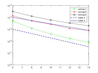
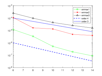
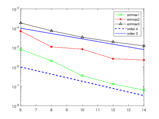
Figure 1: Example 3. The convergence behavior of the absolute cubature errors errmax1, errmax2 and errmax3 for $d=2,\ p=2,$ (a), $d=2,\ p=3$ (b), $d=3,\ p=2$ (c) and $d=3,\ p=3$ (d).

Figure 1 shows the convergence behavior of the absolute cubature errors errmax1, errmax2 and errmax3 for the four considered choices of the pair $(d,p).$ Comparing left and right images of the figure and first referring to ermax2 and errmax3 (i.e. when the rules are applied to singular integrals), we can observe that there is not significant advantage in using $p=3$ instead of $p=2$, either from the point of view of the convergence order or from that of the initial ($N=6$) and final ($N=14$) accuracy. This is a different behavior with respect to Example 2 where the function $f$ was highly smooth everywhere. Referring to errmax1 (i.e. for nearly–singular integrals) however, this comment does not hold anymore.
We observe that for the maximum considered value of $N,$ $N=14,$ we achieve a value for ermax3 of the order of $10^{-5}$ which corresponds to a relative error of the same order; at a first sight this could seem not satisfactory but we remark that the portion of the cylindrical surface taken into account for the integration is quite large. Indeed, repeating the experiment mapping $R_{I}$ to a smaller portion of the surface, the relative error decreases. Finally, comparing top and bottom images we can also conclude that different regularity of the B-spline factor in (1) associated with different choices of $d$ does not significantly influence the accuracy of our rules.

Example 4
In the last example, we consider an integral of interest for the BIE formulation of the 3D Helmholtz problem $\Delta u+k^{2}u=0,$ where $k$ is the wave number defined as $k=2\pi/\lambda,$ with $\lambda$ denoting the wavelength of the electromagnetic radiation. The boundary of the domain of the differential problem is assumed equal to a section of a one sheet hyperboloid which can be parametrically represented as follows,

$${\bf X}({\bf t})=(\cos(\pi t_{1}/4)\sqrt{1+t_{2}^{2}}\,,\,\sin(\pi t_{1}/4)\sqrt{1+t_{2}^{2}}\,,\,t_{2})\,.$$

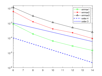
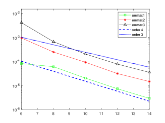
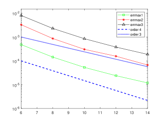
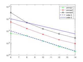
Figure 2: Example 4. The convergence behavior of the absolute cubature errors errmax1, errmax2 and errmax3 for $d=2,\ p=2,$ (a), $d=2,\ p=3$ (b), $d=3,\ p=2$ (c) and $d=3,\ p=3$ (d).

As in the previous example, the integration domain $R_{I}$ is mapped to a quarter of the boundary of the considered section of hyperboloid whose height is $2.$ The matrix $A$ is again defined by the formula in (3) but now the function $f_{\bf s}$ is assigned as follows,

$$f_{\bf s}({\bf t})=J({\bf t})\cos(k\|{\bf X}({\bf t})-{\bf X}({\bf s})\|_{2})\,,$$

with $k=\pi/2$ and $J$ defined as in (12). Note that such function is $C^{1,1}$ also at ${\bf t}={\bf s}.$ The so defined expression of (1) is the real part of the weakly singular integral to be computed when the decomposition in (7) is applied for the Helmholtz kernel on the considered domain and the IgA–BEM collocation approach is adopted for the numerical solution. The results for this example are shown in Figure 2. From the figure we note that in this case increasing $p$ from $2$ to $3$ produced a better accuracy. The errors for the same value of $N$ are a bit worse than those obtained in Example 3. This is due to the more oscillating nature of the function $f_{\bf s}.$ For a different approach to be applied in the nearly singular case with highly oscillating functions see for instance [18].

5 Conclusions

In this paper cubature rules for weakly singular double integrals containing an explicit B-spline factor are presented. The key ideas for these formulas are the extension of a derivative free spline quasi-interpolation scheme and of an algorithm for spline product to the bivariate setting. Numerical results, also of interest in the IgA-BEM setting, confirm good performances of the proposed rules.

References

- [1] Aimi, A., Calabrò F., Diligenti M., Sampoli M.L., Sangalli G., Sestini A.: New efficient assembly in Isogeometric Analysis for Symmetric Galerkin Boundary Element Method, CMAME 331, 327–342 (2018).
- [2] Aimi, A., Diligenti M., Sampoli, M.L., Sestini A.: Isogeometric Analysis and Symmetric Galerkin BEM: a 2D Numerical Study. Applied Mathematics of Computation 272, 173–186 (2016).
- [3] Aimi A., Diligenti M., Sampoli M.L., Sestini A.: Non-polynomial spline alternatives in Isogeometric Symmetric Galerkin BEM, Applied Numerical Mathematics 116, 10–23 (2017).
- [4] Aimi A., Calabrò F., Falini A., Sampoli M.L.: Sestini A.: Quadrature formulas based on spline Quasi-Interpolation for hypersingular integrals rising in IgA-SGBEM, submitted (2019).
- [5] Barrera D., Dagnino C. Ibáñez M.J., Remogna S.: Point and differential quasi-interpolation on three directional meshes, JCAM 354, 373–389 (2019).
- [6] Bonnet, M.: Regular boundary integral equations for three-dimensional finite or infinite bodies with or without curved cracks in elastodynamics, in: C.A. Brebbia, N. Zamani (Eds.), Boundary Element Techniques: Applications in Engineering, Computational Mechanics Publications, pp. 171–188. Southampton, UK (1989).
- [7] Calabrò F., Falini A., Sampoli M.L., Sestini A.: Efficient quadrature rules based on spline quasi-interpolation for application to IGA-BEMs, JCAM 338, 153–167 (2018).
- [8] Costabel, M.: Developments in boundary element methods for time-dependent problems. In: Problems and Methods in Mathematical Physics, Jentsch L., Troltzsch F. (eds), vol. 134, pp. 17–32. Springer, Leipzig (1994).
- [9] Falini A., Giannelli C., Kanduč T., Sampoli M.L., Sestini A.: Isogeometric collocation for 3D BEM: a study on numerical integration with spline quasi-interpolation, in preparation.
- [10] Gao, X.-W.: An effective method for numerical evaluation of general 2D and 3D high order singular boundary integrals, Comput. Methods Appl. Mech. Engrg. 199 2856–2864, (2010).
- [11] Gong, Y.P., Dong, C.Y.: An isogeometric boundary element method using adaptive integral method for 3D potential problems, JCAM 319 141–158 (2017).
- [12] Grošelj J., Speleers H.: Three recipes for quasi-interpolation with cubic Powell–Sabin splines, CAGD 67 47–70, (2018).
- [13] Hsiao, G. C., Wendland, W. L.: Boundary integral equations. Springer, Berlin Heidelberg (2008).
- [14] Klaseboer, E. Fernandez, C., Khoo, B.: A note on true desingularisation of boundary integral methods for three-dimensional potential problems, Engineering Analysis with Boundary Elements 33 (6) 796–801 (2009).
- [15] Manni, C., Pelosi F., Sampoli M.L: Generalized B-splines as a tool in isogemetric analysis, CMAME 200, 867–881 (2011).
- [16] Mazzia F., Sestini A.: The BS class of Hermite spline quasi–interpolants on nonuniform knot distributions, BIT 49 611–629 (2009)
- [17] Mørken, K.: Some identities for products and degree raising of splines, Constr. Approx. 7, 195–208 (1991).
- [18] Occorsio, D., Serafini, G.: Cubature formulae for nearly singular and highly oscillating integrals, Calcolo 55(1), 4 (2018).
- [19] Sablonnière, P.: Recent progress in univariate and multivariate polynomial or spline quasi–interpolants, Trends and Applications in Constructive Approximation, M.G. de Brujn, D. H. Mache and J. Szabados (eds.), Birkh’́auser, Basel, 229–245 (2005).
- [20] Sladek, V., Sladek, J.: Singular Integrals in Boundary Element Methods, WIT Press, Southampton, (1998).
- [21] Schumaker, L. : Spline Functions: Basic Theory, Cambridge Math. Press, 3rd ed. (2007).
- [22] Scuderi, L.: A new smoothing strategy for computing nearly singular integrals in 3D Galerkin BEM, JCAM 225, 406–427 (2009).
- [23] Tan, F., Lv, J., Jiao Y., Liang, J., Zhou, S.: Efficient evaluation of weakly singular integrals with Duffy-distance transformation in 3D BEM, Engineering Analysis with Boundary Elements 104, 63–70 (2019).
- [24] Taus, M., Rodin, G.J., Hughes, T.J.R.: Isogeometric analysis of boundary integral equations: High–order collocation methods for the singular and hyper–singular equations, mathematical Models and Methods in Applied Sciences, 26, 1447–1480 (2016).
- [25] Wendland, W.I.: On some mathematical aspects of boundary element methods for elliptic problems, The Mathematics of Finite Elements and Applications, V. Academic Press, London, 1985.