Obtaining Adjustable Regularization for Free via Iterate Averaging

Jingfeng Wu    Vladimir Braverman    Lin F. Yang
Abstract

Regularization for optimization is a crucial technique to avoid overfitting in machine learning. In order to obtain the best performance, we usually train a model by tuning the regularization parameters. It becomes costly, however, when a single round of training takes significant amount of time. Very recently, Neu & Rosasco (2018) show that if we run stochastic gradient descent (SGD) on linear regression problems, then by averaging the SGD iterates properly, we obtain a regularized solution. It left open whether the same phenomenon can be achieved for other optimization problems and algorithms. In this paper, we establish an averaging scheme that provably converts the iterates of SGD on an arbitrary strongly convex and smooth objective function to its regularized counterpart with an adjustable regularization parameter. Our approaches can be used for accelerated and preconditioned optimization methods as well. We further show that the same methods work empirically on more general optimization objectives including neural networks. In sum, we obtain adjustable regularization for free for a large class of optimization problems and resolve an open question raised by Neu & Rosasco (2018).

Iterate Average, Regularization

1 Introduction

Regularization for optimization is a key technique for avoiding over-fitting in machine learning and statistics  (Grandvalet & Bengio, 2005; Krogh & Hertz, 1992; Tibshirani, 1996; Tikhonov & Arsenin, 1977). The effects of explicit regularization methods, i.e., an extra regularization term added to the vanilla objective, are well studied, e.g., ridge regression (Tikhonov & Arsenin, 1977), LASSO (Tibshirani, 1996) and entropy regularization (Grandvalet & Bengio, 2005). Despite the great benefits of adopting explicit regularization, it could cause a huge computational burden to search for the optimal hyperparameter associated with the extra regularization term, especially for large-scale machine learning problems (Devlin et al., 2018; He et al., 2016; Silver et al., 2017).

In another line of research, people recognize and utilize the implicit regularization caused by certain components in machine learning algorithms, e.g., initialization (He et al., 2015; Hu et al., 2020), batch normalization (Ioffe & Szegedy, 2015; Cai et al., 2018), iterate averaging (Bach & Moulines, 2013; Jain et al., 2018; Neu & Rosasco, 2018), and optimizer such as gradient descent (GD) (Gunasekar et al., 2018; Soudry et al., 2018; Suggala et al., 2018). The regularization effect usually happens along the process of training the model and/or requires little post-computation. A great deal of evidence indicates that such a implicit bias plays a crucial role for the generalization abilities in many modern machine learning models (Zhang et al., 2016; Zhu et al., 2018; Wilson et al., 2017; Soudry et al., 2018). However, the implicit regularization is often a fixed effect and lacks the flexibility to be adjusted. To fully utilize it, we need a thorough understanding about the mechanism of the implicit regularization.

Among all the efforts spent on understanding and utilizing the implicit regularization, the work on bridging iterate averaging with explicit regularization (Neu & Rosasco, 2018) is extraordinarily appealing. In particular, Neu & Rosasco (2018) show that for linear regression, one can achieve 2subscript2\ell_{2}-regularization effect for free by simply taking geometrical averaging over the optimization path generated by stochastic gradient descent (SGD), which costs little additional computation. More interestingly, the regularization is adjustable, i.e., the solution biased by the regularizer in arbitrary strength can be obtained by iterate averaging using the corresponding weighting scheme. In a nutshell, this regularization approach has advantages over both the implicit regularization methods for being adjustable, and the explicit regularization methods for being cheap to tune.

Nevertheless, Neu & Rosasco (2018) only provide a method and its analysis for linear regression optimized by SGD. However linear regression itself is a rather restricted optimization objective. A nature question arises:

Can we obtain “free” and “adjustable” regularization for broader objective functions and optimization methods?

In this work, we answer this question positively from the following aspects:

  1. 1.

    For linear regression, we analyze the regularization effects of averaging the optimization paths of SGD as well as preconditioned SGD, with adaptive learning rates. The averaged solutions achieve effects of 2subscript2\ell_{2}-regularization and generalized 2subscript2\ell_{2}-regularization respectively, in an adjustable manner. Similar results hold for kernel ridge regression as well.

  2. 2.

    We show that for Nesterov’s accelerated stochastic gradient descent, the iterate averaged solution can also realize 2subscript2\ell_{2}-regularization effect by a modified averaging scheme. This resolves an open question raised by Neu & Rosasco (2018).

  3. 3.

    Beside linear regression, we study the regularization effects of iterate averaging for strongly convex and smooth loss functions, hence establishing a provable approach for obtaining nearly free and adjustable regularization for a broad class of functions.

  4. 4.

    Empirical studies on both synthetic and real datasets verify our theory. Moreover, we test iterate averaging with modern deep neural networks on CIFAR-10 and CIFAR-100 datasets, and the proposed approaches still obtain effective and adjustable regularization effects with little additional computation, demonstrating the broad applicability of our methods.

Our analysis is motivated from continuous approximation based on differential equations. When the learning rate tends to zero, the discrete algorithmic iterates tends to be the continuous path of an ordinary differential equation (ODE), on which we can establish a continuous version of our theory. We then discretize the ODE and generalize the theory to that of finite step size. This technique is of independent interests since it can be applied to analyze other comprehensive optimization problems as well (Su et al., 2014; Hu et al., 2017a; Li et al., 2017; Yang et al., 2018; Shi et al., 2019). Our results, in addition to the linear regression result in (Neu & Rosasco, 2018), illustrate the promising application of iterate averaging to obtain adjustable regularization for free.

2 Preliminaries

Let {(xi,yi)d×1}i=1nsuperscriptsubscriptsubscript𝑥𝑖subscript𝑦𝑖superscript𝑑1𝑖1𝑛\{(x_{i},y_{i})\in\mathds{R}^{d\times 1}\}_{i=1}^{n} be the training data and wd𝑤superscript𝑑w\in\mathds{R}^{d} be the parameters to be optimized. The goal is to minimize a lower bounded loss function L(w)𝐿𝑤L(w)

minwL(w):=1ni=1n(xi,yi,w).assignsubscript𝑤𝐿𝑤1𝑛superscriptsubscript𝑖1𝑛subscript𝑥𝑖subscript𝑦𝑖𝑤\displaystyle\min_{w}L(w):=\frac{1}{n}\sum_{i=1}^{n}\ell(x_{i},y_{i},w). (𝒫1subscript𝒫1\mathcal{P}_{1})

One important example is linear regression under the square loss where L(w)=12ni=1nwxiyi22𝐿𝑤12𝑛superscriptsubscript𝑖1𝑛superscriptsubscriptnormsuperscript𝑤topsubscript𝑥𝑖subscript𝑦𝑖22L(w)=\frac{1}{2n}\sum_{i=1}^{n}\left\|w^{\top}x_{i}-y_{i}\right\|_{2}^{2}. The optimization problem often involves an explicit regularization term

minw^L(w^)+λR(w^),subscript^𝑤𝐿^𝑤𝜆𝑅^𝑤\min_{\hat{w}}L(\hat{w})+\lambda R(\hat{w}), (𝒫2subscript𝒫2\mathcal{P}_{2})

where R(w^)𝑅^𝑤R(\hat{w}) is a regularizer and λ𝜆\lambda is the associated hyperparameter. For example, the 2subscript2\ell_{2}-regularizer is R(w^)=12w^22𝑅^𝑤12superscriptsubscriptnorm^𝑤22R(\hat{w})=\frac{1}{2}\left\|\hat{w}\right\|_{2}^{2}. Given an iterative algorithm, e.g., SGD, an optimization path is generated by running the algorithm. With a little abuse of notations, we use {wk}k=0superscriptsubscriptsubscript𝑤𝑘𝑘0\{w_{k}\}_{k=0}^{\infty} and {w^k}k=0superscriptsubscriptsubscript^𝑤𝑘𝑘0\{\hat{w}_{k}\}_{k=0}^{\infty} to represent the optimization paths for the unregularized problem (𝒫1subscript𝒫1\mathcal{P}_{1}) and the regularized problem (𝒫2subscript𝒫2\mathcal{P}_{2}), respectively. Sometimes we write w^ksubscript^𝑤𝑘\hat{w}_{k} with a script as w^k,λsubscript^𝑤𝑘𝜆\hat{w}_{k,\lambda} to emphasize its dependence on the hyperparameter λ𝜆\lambda. We use ηksubscript𝜂𝑘\eta_{k} and γksubscript𝛾𝑘\gamma_{k} to denote the learning rates for training the unregularized and regularized objectives respectively. For simplicity we always initialize the iterative algorithms from zero, i.e., w0=w^0=0subscript𝑤0subscript^𝑤00w_{0}=\hat{w}_{0}=0.

Iterate averaging

The core idea in this work is a technique called iterate averaging. Given a series of parameters {wk}k=0superscriptsubscriptsubscript𝑤𝑘𝑘0\{w_{k}\}_{k=0}^{\infty}, a weighting scheme {pk}k=0superscriptsubscriptsubscript𝑝𝑘𝑘0\{p_{k}\}_{k=0}^{\infty} is defined as a probability distribution associated to the series, i.e., pk0,k=0pk=1formulae-sequencesubscript𝑝𝑘0superscriptsubscript𝑘0subscript𝑝𝑘1p_{k}\geq 0,\ \sum_{k=0}^{\infty}p_{k}=1. Its accumulation is denoted as Pk=i=0kpisubscript𝑃𝑘superscriptsubscript𝑖0𝑘subscript𝑝𝑖P_{k}=\sum_{i=0}^{k}p_{i}, where limkPk=1subscript𝑘subscript𝑃𝑘1\lim_{k\to\infty}P_{k}=1. Since a weighting scheme and its accumulation identifies each other by pk=PkPk1subscript𝑝𝑘subscript𝑃𝑘subscript𝑃𝑘1p_{k}=P_{k}-P_{k-1} for k1𝑘1k\geq 1, we also call {Pk}k=0superscriptsubscriptsubscript𝑃𝑘𝑘0\{P_{k}\}_{k=0}^{\infty} a weighting scheme. Then the iterate averaged parameters are

w~k=Pk1i=0kpiwi,k0.formulae-sequencesubscript~𝑤𝑘superscriptsubscript𝑃𝑘1superscriptsubscript𝑖0𝑘subscript𝑝𝑖subscript𝑤𝑖𝑘0\tilde{w}_{k}={P_{k}}^{-1}{\textstyle\sum}_{i=0}^{k}p_{i}w_{i},\quad k\geq 0.

Various kinds of averaging schemes (for the SGD optimization path) have been studied before. Theoretically, arithmetic averaging is shown to bring better convergence (Bach & Moulines, 2013; Lakshminarayanan & Szepesvari, 2018); tail-averaging is analyzed by Jain et al. (2018); and Neu & Rosasco (2018) discuss geometrically averaging and its regularization effect for SGD and linear regression. Empirically, arithmetic averaging is also shown to be helpful for modern deep neural networks (Izmailov et al., 2018; Zhang et al., 2019; Granziol et al., 2020). Inspired by Neu & Rosasco (2018), in this work we explore in depth the regularization effect induced by iterate averaging for various kinds of optimization algorithms and loss functions.

Stochastic gradient descent

The optimization problem (𝒫1subscript𝒫1\mathcal{P}_{1}) is often solved by stochastic gradient descent (SGD): at every iteration, a mini-batch is sampled uniformly at random, and then the parameters are updated according to the gradient of the loss estimated using the mini-batch. For simplicity we let the batch size be 111. Then with learning rate ηk>0subscript𝜂𝑘0\eta_{k}>0, SGD takes the following update:

wk+1=wkηk(xk,yk,wk).subscript𝑤𝑘1subscript𝑤𝑘subscript𝜂𝑘subscript𝑥𝑘subscript𝑦𝑘subscript𝑤𝑘w_{k+1}=w_{k}-\eta_{k}\operatorname{\nabla}\ell(x_{k},y_{k},w_{k}). (1)

Similarly, for the regularized problem (𝒫2subscript𝒫2\mathcal{P}_{2}), with learning rate γk>0subscript𝛾𝑘0\gamma_{k}>0, SGD takes update:

w^k+1=w^kγk((xk,yk,w^k)+λR(w^k)).subscript^𝑤𝑘1subscript^𝑤𝑘subscript𝛾𝑘subscript𝑥𝑘subscript𝑦𝑘subscript^𝑤𝑘𝜆𝑅subscript^𝑤𝑘\hat{w}_{k+1}=\hat{w}_{k}-\gamma_{k}\left(\operatorname{\nabla}\ell(x_{k},y_{k},\hat{w}_{k})+\lambda\operatorname{\nabla}R(\hat{w}_{k})\right). (2)

For linear regression problem and fixed learning rates, Neu & Rosasco (2018) discuss the geometrically averaging over the SGD iterates (1). They show that by doing so one obtains the solution of the 2subscript2\ell_{2}-regularized problem (𝒫2subscript𝒫2\mathcal{P}_{2}) where R(w^)=12w^22𝑅^𝑤12superscriptsubscriptnorm^𝑤22R(\hat{w})=\frac{1}{2}\left\|\hat{w}\right\|_{2}^{2} for arbitrary hyperparameter λ𝜆\lambda. In this work, we analyze a much broader class of algorithms and functions. In particular, we establish adjustable 2subscript2\ell_{2}-regularization effect for (i) SGD with adaptive learning rate, (ii) kernel ridge regression (Mohri et al., 2018), and (iii) general strongly convex and smooth loss functions.

Preconditioned stochastic gradient descent

We also study iterate averaging for preconditioned stochastic gradient descent (PSGD). Given a positive definite matrix Q𝑄Q as the preconditioning matrix and ηksubscript𝜂𝑘\eta_{k} as the learning rate, the PSGD takes following update to optimize problem (𝒫1subscript𝒫1\mathcal{P}_{1}):

wk+1=wkηkQ1(xk,yk,wk),subscript𝑤𝑘1subscript𝑤𝑘subscript𝜂𝑘superscript𝑄1subscript𝑥𝑘subscript𝑦𝑘subscript𝑤𝑘w_{k+1}=w_{k}-\eta_{k}Q^{-1}\operatorname{\nabla}\ell(x_{k},y_{k},w_{k}), (3)

Similarly, the regularized problem (𝒫2subscript𝒫2\mathcal{P}_{2}) can be solved by PSGD with learning rate γk>0subscript𝛾𝑘0\gamma_{k}>0 as:

w^k+1=w^kγkQ1((xk,yk,w^k)+λR(w^k)).subscript^𝑤𝑘1subscript^𝑤𝑘subscript𝛾𝑘superscript𝑄1subscript𝑥𝑘subscript𝑦𝑘subscript^𝑤𝑘𝜆𝑅subscript^𝑤𝑘\hat{w}_{k+1}=\hat{w}_{k}-\gamma_{k}Q^{-1}\left(\operatorname{\nabla}\ell(x_{k},y_{k},\hat{w}_{k})+\lambda\operatorname{\nabla}R(\hat{w}_{k})\right). (4)

We remark that PSGD unifies several important algorithms as natural gradient descent and Newton’s method at special cases where the curvature matrices can be replaced by constant matrices (Martens, 2014; Dennis Jr & Schnabel, 1996; Bottou & Bousquet, 2008).

For linear regression problems, we will show that geometrically averaging the PSGD iterates (3) leads to a solution biased by the generalized 2subscript2\ell_{2}-regularizer, i.e., the solution of problem (𝒫2subscript𝒫2\mathcal{P}_{2}) with R(w)=12wQw=12wQ2𝑅𝑤12superscript𝑤top𝑄𝑤12superscriptsubscriptnorm𝑤𝑄2R(w)=\frac{1}{2}w^{\top}Qw=\frac{1}{2}\left\|w\right\|_{Q}^{2}. The obtained regularization is adjustable, too.

Nesterov’s accelerated stochastic gradient descent

In problem (𝒫1subscript𝒫1\mathcal{P}_{1}), suppose the loss function L(w)𝐿𝑤L(w) is α𝛼\alpha-strongly convex. Let η>0𝜂0\eta>0 be the learning rate and τ=1ηα1+ηα𝜏1𝜂𝛼1𝜂𝛼\tau=\frac{1-\sqrt{\eta\alpha}}{1+\sqrt{\eta\alpha}}, then the Nesterov’s accelerated stochastic gradient descent (NSGD) takes update (Nesterov, 1983; Su et al., 2014; Yang et al., 2018):

wk+1subscript𝑤𝑘1\displaystyle w_{k+1} =vkη(xk,yk,vk),absentsubscript𝑣𝑘𝜂subscript𝑥𝑘subscript𝑦𝑘subscript𝑣𝑘\displaystyle=v_{k}-\eta\operatorname{\nabla}\ell(x_{k},y_{k},v_{k}), (5)
vksubscript𝑣𝑘\displaystyle v_{k} =wk+τ(wkwk1).absentsubscript𝑤𝑘𝜏subscript𝑤𝑘subscript𝑤𝑘1\displaystyle=w_{k}+\tau(w_{k}-w_{k-1}).

Now we consider the regularized problem (𝒫2subscript𝒫2\mathcal{P}_{2}) with the 2subscript2\ell_{2}-regularizer, R(w^)=12w^22𝑅^𝑤12superscriptsubscriptnorm^𝑤22R(\hat{w})=\frac{1}{2}\left\|\hat{w}\right\|_{2}^{2}. The objective function then becomes (α+λ)𝛼𝜆(\alpha+\lambda)-strongly convex. Let γ>0𝛾0\gamma>0 be the learning rate and τ^=1γ(α+λ)1+γ(α+λ)^𝜏1𝛾𝛼𝜆1𝛾𝛼𝜆\hat{\tau}=\frac{1-\sqrt{\gamma(\alpha+\lambda)}}{1+\sqrt{\gamma(\alpha+\lambda)}}, then the NSGD takes update:

w^k+1subscript^𝑤𝑘1\displaystyle\hat{w}_{k+1} =v^kγ((xk,yk,v^k)+λv^k),absentsubscript^𝑣𝑘𝛾subscript𝑥𝑘subscript𝑦𝑘subscript^𝑣𝑘𝜆subscript^𝑣𝑘\displaystyle=\hat{v}_{k}-\gamma\left(\operatorname{\nabla}\ell(x_{k},y_{k},\hat{v}_{k})+\lambda\hat{v}_{k}\right), (6)
v^ksubscript^𝑣𝑘\displaystyle\hat{v}_{k} =w^k+τ^(w^kw^k1).absentsubscript^𝑤𝑘^𝜏subscript^𝑤𝑘subscript^𝑤𝑘1\displaystyle=\hat{w}_{k}+\hat{\tau}(\hat{w}_{k}-\hat{w}_{k-1}).

It is proposed as an open question by Neu & Rosasco (2018) whether or not adjustable regularization can be obtained by averaging the NSGD optimization path. Our work offers an affirmative answer by showing that for linear regression, one can perform iterate averaging over the NSGD path to obtain the 2subscript2\ell_{2}-regularized solution as well.

3 The free and adjustable regularization induced by iterate averaging

In this section, we show that adjustable regularization effects can be obtained for “free” via iterate averaging for: (i) different SGD schemes, e.g., linear regression or kernel ridge regression with adaptive learning rates; (ii) PSGD; (iii) NSGD; (iv) arbitrary strongly convex and smooth loss functions. Not limited to SGD with fixed learning rate and linear regression, our results manifest the broader potential of employing iterate averaging to obtain regularization that can be tuned with little computation overhead.

Our analysis is motivated from continuous differential equations, which is postponed to Section A of Supplementary Materials due to space limitation. In the following we present our results in discrete cases.

3.1 The effect of an averaged SGD path
Refer to caption
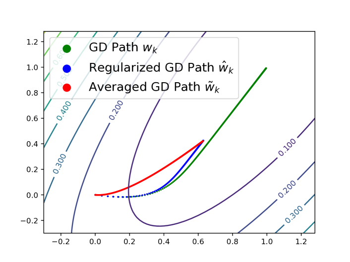
Figure 1: A 2-D demonstration of the effect of an averaged SGD path (Theorem 1). Green dots: the vanilla GD path wksubscript𝑤𝑘w_{k}; blue dots: the regularized GD path w^ksubscript^𝑤𝑘\hat{w}_{k}; red dots: the averaged GD path w~ksubscript~𝑤𝑘\tilde{w}_{k}. The red dots converge to the blue ones.

We first introduce a generalized averaging scheme for the SGD algorithm. Unlike the method in (Neu & Rosasco, 2018), our approach works even with adaptive learning rates. Specifically, given a learning rate schedule and a regularization parameter λ𝜆\lambda, we compute a weighting scheme for averaging a stored SGD path. Then the averaged solution converges to the regularized solution with hyperparameter λ𝜆\lambda. Theorem 1 formally justifies our method.

Theorem 1 (The effect of an averaged SGD path).

Consider loss function L(w)=12ni=1nwxiyi22𝐿𝑤12𝑛superscriptsubscript𝑖1𝑛superscriptsubscriptnormsuperscript𝑤topsubscript𝑥𝑖subscript𝑦𝑖22L(w)=\frac{1}{2n}\sum_{i=1}^{n}\left\|w^{\top}x_{i}-y_{i}\right\|_{2}^{2}, and regularizer R(w)=12w22𝑅𝑤12superscriptsubscriptnorm𝑤22R(w)=\frac{1}{2}\left\|w\right\|_{2}^{2}. Let α𝛼\alpha and β𝛽\beta be such that L(w)𝐿𝑤L(w) is α𝛼\alpha-strongly convex111The strong convexity assumption does not limit the application of our method. For a convex but not strongly convex loss L(w)𝐿𝑤L(w), we can instead collect an optimization path of L(w)+λ0w22𝐿𝑤subscript𝜆0subscriptsuperscriptnorm𝑤22L(w)+\lambda_{0}\left\|w\right\|^{2}_{2} for some small λ0subscript𝜆0\lambda_{0}, which is then strongly convex, and then we apply Theorem 1 to obtain the regularized solutions for a different λ𝜆\lambda. Similar arguments apply to the theorems afterwards as well.and β𝛽\beta-smooth. Let {wk}k=0superscriptsubscriptsubscript𝑤𝑘𝑘0\{w_{k}\}_{k=0}^{\infty} and {w^k}k=0superscriptsubscriptsubscript^𝑤𝑘𝑘0\{\hat{w}_{k}\}_{k=0}^{\infty} be the SGD paths for the vanilla loss function L(w)𝐿𝑤L(w) with learning rate ηksubscript𝜂𝑘\eta_{k}, and the regularized loss function L(w^)+λR(w^)𝐿^𝑤𝜆𝑅^𝑤L(\hat{w})+\lambda R(\hat{w}) with learning rate γksubscript𝛾𝑘\gamma_{k}, respectively. Suppose 1λγk=γk/ηk1𝜆subscript𝛾𝑘subscript𝛾𝑘subscript𝜂𝑘1-\lambda\gamma_{k}={\gamma_{k}}/{\eta_{k}}, ηk(η,1/β)subscript𝜂𝑘𝜂1𝛽\eta_{k}\in(\eta,1/\beta), η>0𝜂0\eta>0 and γ:=η/(1+λη)assign𝛾𝜂1𝜆𝜂\gamma:={\eta}/{(1+\lambda\eta)}. Let

Pk:=i=0kpi=1Πi=0k(γi/ηi).assignsubscript𝑃𝑘superscriptsubscript𝑖0𝑘subscript𝑝𝑖1superscriptsubscriptΠ𝑖0𝑘subscript𝛾𝑖subscript𝜂𝑖P_{k}:={\textstyle\sum}_{i=0}^{k}p_{i}=1-\Pi_{i=0}^{k}({\gamma_{i}}/{\eta_{i}}).

Then for w~k=Pk1i=0kpiwisubscript~𝑤𝑘superscriptsubscript𝑃𝑘1superscriptsubscript𝑖0𝑘subscript𝑝𝑖subscript𝑤𝑖\tilde{w}_{k}=P_{k}^{-1}\sum_{i=0}^{k}p_{i}w_{i} we have

1. Pk𝔼[w~k]=𝔼[w^k](1Pk)𝔼[wk]subscript𝑃𝑘𝔼delimited-[]subscript~𝑤𝑘𝔼delimited-[]subscript^𝑤𝑘1subscript𝑃𝑘𝔼delimited-[]subscript𝑤𝑘P_{k}\cdot\mathds{E}[\tilde{w}_{k}]=\mathds{E}[\hat{w}_{k}]-(1-P_{k})\cdot\mathds{E}[w_{k}].

2. Both 𝔼[wk]𝔼delimited-[]subscript𝑤𝑘\mathds{E}[w_{k}] and 𝔼[w^k]𝔼delimited-[]subscript^𝑤𝑘\mathds{E}[\hat{w}_{k}] converge. Moreover, we have 𝔼[w^k]𝔼[w~k]2𝒪((1λγ)k)subscriptnorm𝔼delimited-[]subscript^𝑤𝑘𝔼delimited-[]subscript~𝑤𝑘2𝒪superscript1𝜆𝛾𝑘\left\|\mathds{E}[\hat{w}_{k}]-\mathds{E}[\tilde{w}_{k}]\right\|_{2}\leq\mathcal{O}((1-\lambda\gamma)^{k}).

3. If the gradient noise ϵk=(xk,yk,w)L(w)subscriptitalic-ϵ𝑘subscript𝑥𝑘subscript𝑦𝑘𝑤𝐿𝑤\epsilon_{k}=\operatorname{\nabla}\ell(x_{k},y_{k},w)-\operatorname{\nabla}L(w) has uniformly bounded variance 𝔼[ϵk22]σ2𝔼delimited-[]superscriptsubscriptnormsubscriptitalic-ϵ𝑘22superscript𝜎2\mathds{E}[\left\|\epsilon_{k}\right\|_{2}^{2}]\leq\sigma^{2}, then for k𝑘k large enough, with probability at least 1δ1𝛿1-\delta we have222In this high probability result, the confidence parameter δ𝛿\delta appears in a polynomial order, 1δ1𝛿\frac{1}{\sqrt{\delta}}. However this is only due to the assumption of bounded variance of the noise and an application of Chebyshev’s inequality. It is straightforward to obtain a logarithm dependence on δ𝛿\delta by assuming the sub-Gaussianity of the noise and applying Hoeffding’s inequality. Similar arguments apply to the theorems afterwards as well.

Pkw~kPk𝔼[w~k]2ϵ,subscriptnormsubscript𝑃𝑘subscript~𝑤𝑘subscript𝑃𝑘𝔼delimited-[]subscript~𝑤𝑘2italic-ϵ\left\|P_{k}\tilde{w}_{k}-P_{k}\mathds{E}[\tilde{w}_{k}]\right\|_{2}\leq\epsilon,

where ϵ=σγ(λ+α)(λ+β)2italic-ϵ𝜎𝛾𝜆𝛼superscript𝜆𝛽2\epsilon=\frac{\sigma}{\gamma(\lambda+\alpha)(\lambda+\beta)^{2}} λδγ(2λγ)absent𝜆𝛿𝛾2𝜆𝛾\cdot\sqrt{\frac{\lambda}{\delta\gamma(2-\lambda\gamma)}}.

The proof is left in Supplementary Materials, Section C.1. A 2-D illustration for Theorem 1 is presented in Figure 1.

Theorem 1 guarantees the method of obtaining adjustable 2subscript2\ell_{2}-regularization for free via iterate averaging. Specifically, we first collect an SGD path {wk}k=0superscriptsubscriptsubscript𝑤𝑘𝑘0\left\{w_{k}\right\}_{k=0}^{\infty} for L(w)𝐿𝑤L(w) under a learning rate schedule ηksubscript𝜂𝑘\eta_{k} (it can be chosen in a broad range); then for a regularization parameter λ𝜆\lambda, we compute an averaging scheme {pk}k=0superscriptsubscriptsubscript𝑝𝑘𝑘0\left\{p_{k}\right\}_{k=0}^{\infty} that converts the collected SGD path to the regularized solution, w^subscript^𝑤\hat{w}_{\infty}. Note that the learning rate schedule γksubscript𝛾𝑘\gamma_{k} is only for analysis and does not need to be known.

Specifically, when the learning rates are constants, i.e., ηi=ηsubscript𝜂𝑖𝜂\eta_{i}=\eta and γi=γsubscript𝛾𝑖𝛾\gamma_{i}=\gamma, the first two conclusions in Theorem 1 recover the Proposition 1 and Proposition 2 in (Neu & Rosasco, 2018). Besides, the third claim in Theorem 1 characterizes the deviation of the averaged solution, which relies on the models, learning rates, and the regularization parameter, etc. And empirical studies in Section 4.2 do suggest that such a deviation is sufficiently small that it does not affect the induced regularization effect.

Remark.

We emphasize that the method of Neu & Rosasco (2018) only applies to SGD with constant learning rate. Moreover, their theory only guarantees the averaged solution has convergence in expectation, which is not very useful since the averaged solution might not converge to the regularized solution almost surely, not even in probability (a.k.a. weak convergence) (see Section 4.2). Nevertheless, our theory carefully characterizes the deviation between the averaged solution and the regularized solution.

More interestingly, Theorem 1.1 shows that this method is also applicable to kernel ridge regression (in the dual space).

Theorem 1.1.

Let Kn×n𝐾superscript𝑛𝑛K\in\mathds{R}^{n\times n} be a kernel, K(i,j)=ϕ(xi)ϕ(xj)𝐾𝑖𝑗italic-ϕsuperscriptsubscript𝑥𝑖topitalic-ϕsubscript𝑥𝑗K(i,j)=\phi(x_{i})^{\top}\phi(x_{j}), where ϕ:d:italic-ϕsuperscript𝑑\phi:\mathds{R}^{d}\to\mathcal{H} is the kernel map. Consider kernel ridge regression

minαnL(α,λ):=12yKα22+λ2αKαassignsubscript𝛼superscript𝑛𝐿𝛼𝜆12superscriptsubscriptnorm𝑦𝐾𝛼22𝜆2superscript𝛼top𝐾𝛼\min_{\alpha\in\mathds{R}^{n}}L(\alpha,\lambda):=\frac{1}{2}\left\|y-K\alpha\right\|_{2}^{2}+\frac{\lambda}{2}\alpha^{\top}K\alpha

where y=(y1,,yn)T𝑦superscriptsubscript𝑦1subscript𝑦𝑛𝑇y=(y_{1},\dots,y_{n})^{T} is the labels and αn𝛼superscript𝑛\alpha\in\mathds{R}^{n} is the dual parameter. Let {αk}k=0superscriptsubscriptsubscript𝛼𝑘𝑘0\{\alpha_{k}\}_{k=0}^{\infty} and {α^k}k=0superscriptsubscriptsubscript^𝛼𝑘𝑘0\{\hat{\alpha}_{k}\}_{k=0}^{\infty} be the GD paths for the loss L(α,λ)𝐿𝛼𝜆L(\alpha,\lambda) with learning rate ηksubscript𝜂𝑘\eta_{k}, and the loss L(α^,λ^)𝐿^𝛼^𝜆L(\hat{\alpha},\hat{\lambda}) with generalized learning rate γksubscript𝛾𝑘\gamma_{k}, respectively. Suppose λ^>λ^𝜆𝜆\hat{\lambda}>\lambda, γk=ηk(I+(λ^λ)ηkK)1subscript𝛾𝑘subscript𝜂𝑘superscript𝐼^𝜆𝜆subscript𝜂𝑘𝐾1\gamma_{k}=\eta_{k}\left(I+(\hat{\lambda}-\lambda)\eta_{k}K\right)^{-1}. Let

Pk:=i=0kpi=1Πi=0k(γi/ηi).assignsubscript𝑃𝑘superscriptsubscript𝑖0𝑘subscript𝑝𝑖1superscriptsubscriptΠ𝑖0𝑘subscript𝛾𝑖subscript𝜂𝑖P_{k}:={\textstyle\sum}_{i=0}^{k}p_{i}=1-\Pi_{i=0}^{k}\left(\gamma_{i}/\eta_{i}\right).

Then for α~k=Pk1i=0kpiαisubscript~𝛼𝑘superscriptsubscript𝑃𝑘1superscriptsubscript𝑖0𝑘subscript𝑝𝑖subscript𝛼𝑖\tilde{\alpha}_{k}=P_{k}^{-1}\sum_{i=0}^{k}p_{i}\alpha_{i} we have

1. Pkα~k=α^k(1Pk)αksubscript𝑃𝑘subscript~𝛼𝑘subscript^𝛼𝑘1subscript𝑃𝑘subscript𝛼𝑘P_{k}\tilde{\alpha}_{k}=\hat{\alpha}_{k}-(1-P_{k})\alpha_{k}.

2. Both αksubscript𝛼𝑘\alpha_{k} and α^ksubscript^𝛼𝑘\hat{\alpha}_{k} converge provided suitable learning rates. Moreover, we have α^kα~k2𝒪(Ck)subscriptnormsubscript^𝛼𝑘subscript~𝛼𝑘2𝒪superscript𝐶𝑘\left\|\hat{\alpha}_{k}-\tilde{\alpha}_{k}\right\|_{2}\leq\mathcal{O}(C^{k}) where C(0,1)𝐶01C\in(0,1) is a constant decided by K𝐾K, λ^λ^𝜆𝜆\hat{\lambda}-\lambda and ηksubscript𝜂𝑘\eta_{k}.

3.2 The effect of an averaged PSGD path
Refer to caption
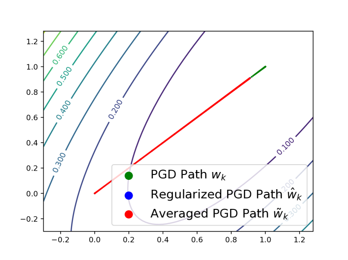
Figure 2: A 2-D demonstration of the effect of an averaged PSGD path (Theorem 2). The Hessian is used as the preconditioning matrix. Green dots: the vanilla PGD path wtsubscript𝑤𝑡w_{t}; blue dots: the regularized PGD path w^tsubscript^𝑤𝑡\hat{w}_{t}; red dots: the averaged PGD path w~tsubscript~𝑤𝑡\tilde{w}_{t}. The red dots converge to the blue ones.

In practice, we usually need many different regularizers. And one important class of them is the generalized 2subscript2\ell_{2}-regularizers, i.e., R(w):=12wQwassign𝑅𝑤12superscript𝑤top𝑄𝑤R(w):=\frac{1}{2}w^{\top}Qw for some positive definite matrix Q𝑄Q. But it is painful to adjust its regularization parameter λ𝜆\lambda by re-training the model. Luckily, we show that the solution biased by such a regularizer can also be obtained for “free” by averaging the optimization path of PSGD. Our result is formally presented in the next theorem.

Theorem 2 (The effect of an averaged PSGD path).

Consider loss function L(w)=12ni=1nwxiyi22𝐿𝑤12𝑛superscriptsubscript𝑖1𝑛superscriptsubscriptnormsuperscript𝑤topsubscript𝑥𝑖subscript𝑦𝑖22L(w)=\frac{1}{2n}\sum_{i=1}^{n}\left\|w^{\top}x_{i}-y_{i}\right\|_{2}^{2}, and regularizer R(w)=12wQw𝑅𝑤12superscript𝑤top𝑄𝑤R(w)=\frac{1}{2}w^{\top}Qw, where Q𝑄Q is a positive definite matrix. Let α𝛼\alpha and β𝛽\beta be such that αQΣ=n1i=1nxixiβQprecedes-or-equals𝛼𝑄Σsuperscript𝑛1superscriptsubscript𝑖1𝑛subscript𝑥𝑖superscriptsubscript𝑥𝑖topprecedes-or-equals𝛽𝑄\alpha Q\preceq\Sigma=n^{-1}\sum_{i=1}^{n}x_{i}x_{i}^{\top}\preceq\beta Q. With Q𝑄Q as the preconditioning matrix, let {wk}k=0superscriptsubscriptsubscript𝑤𝑘𝑘0\{w_{k}\}_{k=0}^{\infty} and {w^k}k=0superscriptsubscriptsubscript^𝑤𝑘𝑘0\{\hat{w}_{k}\}_{k=0}^{\infty} be the PSGD paths for the vanilla loss function L(w)𝐿𝑤L(w) with learning rate ηksubscript𝜂𝑘\eta_{k}, and the regularized loss function L(w^)+λR(w^)𝐿^𝑤𝜆𝑅^𝑤L(\hat{w})+\lambda R(\hat{w}) with learning rate γksubscript𝛾𝑘\gamma_{k}, respectively. Suppose 1λγk=γk/ηk1𝜆subscript𝛾𝑘subscript𝛾𝑘subscript𝜂𝑘1-\lambda\gamma_{k}={\gamma_{k}}/{\eta_{k}}, ηk(η,1/β)subscript𝜂𝑘𝜂1𝛽\eta_{k}\in(\eta,1/\beta), η>0𝜂0\eta>0 and γ:=η/(1+λη)assign𝛾𝜂1𝜆𝜂\gamma:={\eta}/{(1+\lambda\eta)}. Let

Pk:=i=0kpi=1Πi=0k(γi/ηi).assignsubscript𝑃𝑘superscriptsubscript𝑖0𝑘subscript𝑝𝑖1superscriptsubscriptΠ𝑖0𝑘subscript𝛾𝑖subscript𝜂𝑖P_{k}:={\textstyle\sum}_{i=0}^{k}p_{i}=1-\Pi_{i=0}^{k}({\gamma_{i}}/{\eta_{i}}).

Then for w~k=Pk1i=0kpiwisubscript~𝑤𝑘superscriptsubscript𝑃𝑘1superscriptsubscript𝑖0𝑘subscript𝑝𝑖subscript𝑤𝑖\tilde{w}_{k}=P_{k}^{-1}\sum_{i=0}^{k}p_{i}w_{i} we have

1. Pk𝔼[w~k]=𝔼[w^k](1Pk)𝔼[wk]subscript𝑃𝑘𝔼delimited-[]subscript~𝑤𝑘𝔼delimited-[]subscript^𝑤𝑘1subscript𝑃𝑘𝔼delimited-[]subscript𝑤𝑘P_{k}\cdot\mathds{E}[\tilde{w}_{k}]=\mathds{E}[\hat{w}_{k}]-(1-P_{k})\cdot\mathds{E}[w_{k}].

2. Both 𝔼[wk]𝔼delimited-[]subscript𝑤𝑘\mathds{E}[w_{k}] and 𝔼[w^k]𝔼delimited-[]subscript^𝑤𝑘\mathds{E}[\hat{w}_{k}] converge. Moreover, we have 𝔼[w^k]𝔼[w~k]2𝒪((1λγ)k)subscriptnorm𝔼delimited-[]subscript^𝑤𝑘𝔼delimited-[]subscript~𝑤𝑘2𝒪superscript1𝜆𝛾𝑘\left\|\mathds{E}[\hat{w}_{k}]-\mathds{E}[\tilde{w}_{k}]\right\|_{2}\leq\mathcal{O}((1-\lambda\gamma)^{k}).

3. If the noise ϵk=Q1((xk,yk,w)L(w))subscriptitalic-ϵ𝑘superscript𝑄1subscript𝑥𝑘subscript𝑦𝑘𝑤𝐿𝑤\epsilon_{k}=Q^{-1}(\operatorname{\nabla}\ell(x_{k},y_{k},w)-\operatorname{\nabla}L(w)) has uniform bounded variance 𝔼[ϵk22]σ2𝔼delimited-[]superscriptsubscriptnormsubscriptitalic-ϵ𝑘22superscript𝜎2\mathds{E}[\left\|\epsilon_{k}\right\|_{2}^{2}]\leq\sigma^{2}, then for k𝑘k large enough, with probability at least 1δ1𝛿1-\delta we have

Pkw~kPk𝔼[w~k]2ϵ,subscriptnormsubscript𝑃𝑘subscript~𝑤𝑘subscript𝑃𝑘𝔼delimited-[]subscript~𝑤𝑘2italic-ϵ\left\|P_{k}\tilde{w}_{k}-P_{k}\mathds{E}[\tilde{w}_{k}]\right\|_{2}\leq\epsilon,

where ϵ=σQ2γ(λ+α)(λ+β)2λδγ(2λγ)italic-ϵ𝜎subscriptnorm𝑄2𝛾𝜆𝛼superscript𝜆𝛽2𝜆𝛿𝛾2𝜆𝛾\epsilon=\frac{\sigma\left\|Q\right\|_{2}}{\gamma(\lambda+\alpha)(\lambda+\beta)^{2}}\sqrt{\frac{\lambda}{\delta\gamma(2-\lambda\gamma)}}.

The proof is left in Supplementary Materials, Section C.3. A 2-D illustration for Theorem 2 is presented in Figure 2.

The importance of Theorem 2 is two-folds. On the one hand, averaging the PSGD path has an effect as the generalized 2subscript2\ell_{2}-regularizer. And as before, this induced regularization is both adjustable and costless. The considered PSGD algorithm applies to natural gradient descent and Newton’s method in certain circumstances where the curvature matrices can be replaced by constant matrices (Martens, 2014; Dennis Jr & Schnabel, 1996; Bottou & Bousquet, 2008). On the other hand, to obtain a desired type of generalized 2subscript2\ell_{2}-regularization effect, we should store and average a PSGD path with the corresponding preconditioning matrix as indicated in Theorem 2, instead of using a SGD path.

3.3 The effect of an averaged NSGD path
Refer to caption
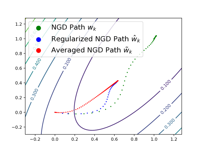
Figure 3: A 2-D demonstration of the effect of an averaged NSGD path (Theorem 3). Green dots: the vanilla NGD path wtsubscript𝑤𝑡w_{t}; blue dots: the regularized NGD path w^tsubscript^𝑤𝑡\hat{w}_{t}; red dots: the averaged NGD path w~tsubscript~𝑤𝑡\tilde{w}_{t}. The red dots converge to the blue ones.

In this part, we show how to obtain adjustable regularization effect by applying averaging schemes on the NSGD path.

Theorem 3 (The effect of an averaged NSGD path).

Consider loss function L(w)=12ni=1nwxiyi22𝐿𝑤12𝑛superscriptsubscript𝑖1𝑛superscriptsubscriptnormsuperscript𝑤topsubscript𝑥𝑖subscript𝑦𝑖22L(w)=\frac{1}{2n}\sum_{i=1}^{n}\left\|w^{\top}x_{i}-y_{i}\right\|_{2}^{2}, and regularizer R(w)=12w22𝑅𝑤12superscriptsubscriptnorm𝑤22R(w)=\frac{1}{2}\left\|w\right\|_{2}^{2}. Let α𝛼\alpha and β𝛽\beta be such that L(w)𝐿𝑤L(w) is α𝛼\alpha-strongly convex and β𝛽\beta-smooth. Let {wk}k=0superscriptsubscriptsubscript𝑤𝑘𝑘0\{w_{k}\}_{k=0}^{\infty} and {w^k}k=0superscriptsubscriptsubscript^𝑤𝑘𝑘0\{\hat{w}_{k}\}_{k=0}^{\infty} be the NSGD paths for the vanilla loss function L(w)𝐿𝑤L(w) with learning rate η𝜂\eta, and the regularized loss function L(w^)+λR(w^)𝐿^𝑤𝜆𝑅^𝑤L(\hat{w})+\lambda R(\hat{w}) with learning rate γ𝛾\gamma, respectively. Suppose 1λγ=γ/η1𝜆𝛾𝛾𝜂1-\lambda\gamma={\gamma}/{\eta}, η(0,1/β)𝜂01𝛽\eta\in(0,1/\beta). Let

Pk:=i=0kpk=1γη(1γ(α+λ)1ηα)k1.assignsubscript𝑃𝑘superscriptsubscript𝑖0𝑘subscript𝑝𝑘1𝛾𝜂superscript1𝛾𝛼𝜆1𝜂𝛼𝑘1P_{k}:=\sum_{i=0}^{k}p_{k}=1-\frac{\gamma}{\eta}\left(\frac{1-\sqrt{\gamma(\alpha+\lambda)}}{1-\sqrt{\eta\alpha}}\right)^{k-1}.

Then for w~k=Pk1i=0kpiwisubscript~𝑤𝑘superscriptsubscript𝑃𝑘1superscriptsubscript𝑖0𝑘subscript𝑝𝑖subscript𝑤𝑖\tilde{w}_{k}=P_{k}^{-1}\sum_{i=0}^{k}p_{i}w_{i} we have

1. Pk𝔼[w~k]=𝔼[w^k](1Pk)𝔼[wk]subscript𝑃𝑘𝔼delimited-[]subscript~𝑤𝑘𝔼delimited-[]subscript^𝑤𝑘1subscript𝑃𝑘𝔼delimited-[]subscript𝑤𝑘P_{k}\cdot\mathds{E}[\tilde{w}_{k}]=\mathds{E}[\hat{w}_{k}]-(1-P_{k})\cdot\mathds{E}[w_{k}].

2. 𝔼[wk]𝔼delimited-[]subscript𝑤𝑘\mathds{E}[w_{k}] and 𝔼[w^k]𝔼delimited-[]subscript^𝑤𝑘\mathds{E}[\hat{w}_{k}] converge. And 𝔼[w^k]𝔼[w~k]2𝒪(Ck)subscriptnorm𝔼delimited-[]subscript^𝑤𝑘𝔼delimited-[]subscript~𝑤𝑘2𝒪superscript𝐶𝑘\left\|\mathds{E}[\hat{w}_{k}]-\mathds{E}[\tilde{w}_{k}]\right\|_{2}\leq\mathcal{O}\left(C^{k}\right), where C=1γ(α+λ)1ηα(0,1)𝐶1𝛾𝛼𝜆1𝜂𝛼01C=\frac{1-\sqrt{\gamma(\alpha+\lambda)}}{1-\sqrt{\eta\alpha}}\in(0,1).

3. If the gradient noise ϵk=(xk,yk,w)L(w)subscriptitalic-ϵ𝑘subscript𝑥𝑘subscript𝑦𝑘𝑤𝐿𝑤\epsilon_{k}=\operatorname{\nabla}\ell(x_{k},y_{k},w)-\operatorname{\nabla}L(w) has uniformly bounded variance 𝔼[ϵk22]σ2𝔼delimited-[]superscriptsubscriptnormsubscriptitalic-ϵ𝑘22superscript𝜎2\mathds{E}[\left\|\epsilon_{k}\right\|_{2}^{2}]\leq\sigma^{2}, then for k𝑘k large enough, with probability at least 1δ1𝛿1-\delta we have

Pkw~kPk𝔼[w~k]2ϵ,subscriptnormsubscript𝑃𝑘subscript~𝑤𝑘subscript𝑃𝑘𝔼delimited-[]subscript~𝑤𝑘2italic-ϵ\left\|P_{k}\tilde{w}_{k}-P_{k}\mathds{E}[\tilde{w}_{k}]\right\|_{2}\leq\epsilon,

where ϵitalic-ϵ\epsilon depends on σ,α,β,η,γ𝜎𝛼𝛽𝜂𝛾\sigma,\alpha,\beta,\eta,\gamma.

The proof and the exact value of ϵitalic-ϵ\epsilon are given in Supplementary Materials, Section C.4. A 2-D illustration for Theorem 3 is presented in Figure 3.

Theorem 3 affirmatively answers an open question raised by Neu & Rosasco (2018): there exists an averaging scheme for NSGD to achieve 2subscript2\ell_{2}-regularization in arbitrary strength. In addition to the results for averaging SGD, Theorem 3 provides us wider choices of applicable optimizers for obtaining adjustable 2subscript2\ell_{2}-regularization effect by iterate averaging.

3.4 The effect of an averaged GD path for strongly convex and smooth loss functions

In this section, we show that the iterate averaging methods work for not only simple optimization objectives like least square, but also a much broader set of loss functions. In fact, we show that any strongly convex and smooth function admits an iterate averaging scheme, which brings 2subscript2\ell_{2}-regularization effect in a tunable manner. More formally, in the problems (𝒫1subscript𝒫1\mathcal{P}_{1}) and (𝒫2subscript𝒫2\mathcal{P}_{2}), let L(w)𝐿𝑤L(w) be α𝛼\alpha-strongly convex and β𝛽\beta-smooth, and R(w):=12w22assign𝑅𝑤12superscriptsubscriptnorm𝑤22R(w):=\frac{1}{2}\left\|w\right\|_{2}^{2} be the 2subscript2\ell_{2}-regularizer. For the sake of representation, we focus on gradient descent (GD) with constant learning rate applied on the loss functions. Similar arguments can also be applied for SGD, PSGD and NSGD. The GD takes update

wk+1=wkηL(wk),subscript𝑤𝑘1subscript𝑤𝑘𝜂𝐿subscript𝑤𝑘\displaystyle w_{k+1}=w_{k}-\eta\operatorname{\nabla}L(w_{k}),
w^k+1,λ=w^k,λγ(L(w^k,λ)+λw^k,λ),subscript^𝑤𝑘1𝜆subscript^𝑤𝑘𝜆𝛾𝐿subscript^𝑤𝑘𝜆𝜆subscript^𝑤𝑘𝜆\displaystyle\hat{w}_{k+1,\lambda}=\hat{w}_{k,\lambda}-\gamma(\operatorname{\nabla}L(\hat{w}_{k,\lambda})+\lambda\hat{w}_{k,\lambda}),

for optimizing problems (𝒫1subscript𝒫1\mathcal{P}_{1}) and (𝒫2subscript𝒫2\mathcal{P}_{2}), respectively. Let b=L(w0)=L(0)𝑏𝐿subscript𝑤0𝐿0b=-\operatorname{\nabla}L(w_{0})=-\operatorname{\nabla}L(0). Let us denote two iterations

uk+1uk=η(αukb),vk+1vk=η(βvkb),formulae-sequencesubscript𝑢𝑘1subscript𝑢𝑘𝜂𝛼subscript𝑢𝑘𝑏subscript𝑣𝑘1subscript𝑣𝑘𝜂𝛽subscript𝑣𝑘𝑏u_{k+1}-u_{k}=-\eta(\alpha u_{k}-b),\quad v_{k+1}-v_{k}=-\eta(\beta v_{k}-b),

where u0=v0=0subscript𝑢0subscript𝑣00u_{0}=v_{0}=0. Consider an averaging scheme Pk=i=0kpi=1(γ/η)k+1subscript𝑃𝑘superscriptsubscript𝑖0𝑘subscript𝑝𝑖1superscript𝛾𝜂𝑘1P_{k}=\sum_{i=0}^{k}p_{i}=1-\left({\gamma}/{\eta}\right)^{k+1}. Let u~k=Pk1i=0kpiuisubscript~𝑢𝑘superscriptsubscript𝑃𝑘1superscriptsubscript𝑖0𝑘subscript𝑝𝑖subscript𝑢𝑖\tilde{u}_{k}={P_{k}}^{-1}\sum_{i=0}^{k}p_{i}u_{i}, v~k=Pk1i=0kpivisubscript~𝑣𝑘superscriptsubscript𝑃𝑘1superscriptsubscript𝑖0𝑘subscript𝑝𝑖subscript𝑣𝑖\tilde{v}_{k}={P_{k}}^{-1}\sum_{i=0}^{k}p_{i}v_{i}, and w~k=Pk1i=0kpiwisubscript~𝑤𝑘superscriptsubscript𝑃𝑘1superscriptsubscript𝑖0𝑘subscript𝑝𝑖subscript𝑤𝑖\tilde{w}_{k}=P_{k}^{-1}\sum_{i=0}^{k}p_{i}w_{i}. Then the next theorem characterizes the regularization effect of a averaged GD path for general strongly convex and smooth loss functions.

Theorem 4 (The effect of an averaged GD path for strongly convex and smooth loss functions).

Without loss of generality, assume the unique minimum wsubscript𝑤w_{*} of L(w)𝐿𝑤L(w) satisfies w>w0=0subscript𝑤subscript𝑤00w_{*}>w_{0}=0 entry-wisely. Suppose 1/(2βα)<η<1/β12𝛽𝛼𝜂1𝛽{1}/{(2\beta-\alpha)}<\eta<{1}/{\beta}, 0<γ<η/(η(βα)+1)0𝛾𝜂𝜂𝛽𝛼10<\gamma<{\eta}/{(\eta(\beta-\alpha)+1)}. Then for hyperparameters

λ1=1/γ1/η+βα,λ2=1/γ1/η+αβ,formulae-sequencesubscript𝜆11𝛾1𝜂𝛽𝛼subscript𝜆21𝛾1𝜂𝛼𝛽\lambda_{1}={1}/{\gamma}-{1}/{\eta}+\beta-\alpha,\quad\lambda_{2}={1}/{\gamma}-{1}/{\eta}+\alpha-\beta,

we have

1. w^k,λ1+(1Pk)(v~kvk)w~kw^k,λ2+(1Pk)(u~kuk)subscript^𝑤𝑘subscript𝜆11subscript𝑃𝑘subscript~𝑣𝑘subscript𝑣𝑘subscript~𝑤𝑘subscript^𝑤𝑘subscript𝜆21subscript𝑃𝑘subscript~𝑢𝑘subscript𝑢𝑘\hat{w}_{k,\lambda_{1}}+(1-P_{k})(\tilde{v}_{k}-v_{k})\leq\tilde{w}_{k}\leq\hat{w}_{k,\lambda_{2}}+(1-P_{k})(\tilde{u}_{k}-u_{k}), where the “\leq” is defined entry-wisely.

2. uk,u~k,vk,v~k,w^k,λ1,w^k,λ2subscript𝑢𝑘subscript~𝑢𝑘subscript𝑣𝑘subscript~𝑣𝑘subscript^𝑤𝑘subscript𝜆1subscript^𝑤𝑘subscript𝜆2u_{k},\tilde{u}_{k},v_{k},\tilde{v}_{k},\hat{w}_{k,\lambda_{1}},\hat{w}_{k,\lambda_{2}} converge. Moreover let m=(w^,λ2+w^,λ1)/2𝑚subscript^𝑤subscript𝜆2subscript^𝑤subscript𝜆12m=(\hat{w}_{\infty,\lambda_{2}}+\hat{w}_{\infty,\lambda_{1}})/2, d=(w^,λ2w^,λ1)/2𝑑subscript^𝑤subscript𝜆2subscript^𝑤subscript𝜆12d=(\hat{w}_{\infty,\lambda_{2}}-\hat{w}_{\infty,\lambda_{1}})/2 and C=max{(1γ(α+λ1),(1γ(α+λ2),γη}(0,1)C=\max\{(1-\gamma(\alpha+\lambda_{1}),(1-\gamma(\alpha+\lambda_{2}),\frac{\gamma}{\eta}\}\in(0,1), then w~km2d2+𝒪(Ck)subscriptnormsubscript~𝑤𝑘𝑚2subscriptnorm𝑑2𝒪superscript𝐶𝑘\left\|\tilde{w}_{k}-m\right\|_{2}\leq\left\|d\right\|_{2}+\mathcal{O}(C^{k}).

The proof is left in Supplementary Materials, Section C.5 .

According to Theorem 4, for strongly convex and smooth objectives, the averaged GD path {w~k}k=0superscriptsubscriptsubscript~𝑤𝑘𝑘0\{\tilde{w}_{k}\}_{k=0}^{\infty} lies in the area between two regularized GD paths, {w^k,λ1}k=0superscriptsubscriptsubscript^𝑤𝑘subscript𝜆1𝑘0\{\hat{w}_{k,\lambda_{1}}\}_{k=0}^{\infty} and {w^k,λ2}k=0superscriptsubscriptsubscript^𝑤𝑘subscript𝜆2𝑘0\{\hat{w}_{k,\lambda_{2}}\}_{k=0}^{\infty}. Furthermore, w~ksubscript~𝑤𝑘\tilde{w}_{k} converges to a hyper cube whose diagonal vertices are defined by w^,λ1subscript^𝑤subscript𝜆1\hat{w}_{\infty,\lambda_{1}} and w^,λ2subscript^𝑤subscript𝜆2\hat{w}_{\infty,\lambda_{2}}. In this way for this class of loss functions, averaging the GD path has an “approximate” 2subscript2\ell_{2}-regularization effect that is in between two 2subscript2\ell_{2}-regularizers with hyperparameters as λ1subscript𝜆1\lambda_{1} and λ2subscript𝜆2\lambda_{2} respectively. In addition, λ1subscript𝜆1\lambda_{1} and λ2subscript𝜆2\lambda_{2} can be adjusted through changing the weighting scheme. Finally, we note that d2=𝒪(βα)subscriptnorm𝑑2𝒪𝛽𝛼\left\|d\right\|_{2}=\operatorname{\mathcal{O}}\left(\beta-\alpha\right), thus when the objective is quadratic, we have α=β𝛼𝛽\alpha=\beta and d=0𝑑0d=0 and thus the “approximate” 2subscript2\ell_{2}-regularization effect becomes the exact 2subscript2\ell_{2}-regularization by Theorem 4.

We therefore conjecture that, generally, for arbitrary loss functions and iterative optimizers, an iterate averaging scheme admits a specific yet unknown regularization effect. Indeed, our experiments in the next section empirically verifies such an effect by performing iterate averaging on deep neural networks, which are highly comprehensive.

4 Experiments

In this section we present our empirical studies. The detailed setups are explained in Supplementary Materials, Section D. The code is available at https://github.com/uuujf/IterAvg.

4.1 Two dimensional demonstration

We first introduce a two dimensional toy example to demonstrate the regularization effect of iterate averaging. The vanilla loss function is quadratic with a unique minimum at (1,1)11(1,1), as shown in Figure 1similar-to\sim3. For the purpose of demonstration we only run deterministic algorithms with constant learning rates. We plot the trajectories of the concerned optimizers for learning the vanilla loss function and the regularized loss function, as well as the averaged solutions. All of the optimizers start iterations from zero.

In Figure 1, the green and the blue dots represent the GD paths for optimizing the vanilla/regularized loss functions respectively, while the red dots are the path of iterate averaged solutions. We observe that the red dots do converge to the blue ones, indicating the averaged solution has the same effect of an 2subscript2\ell_{2}-regularizer, as suggested by Theorem 1. Similarly the phenomenon holds for averaging the NGD path, as indicated in Figure 3. In Figure 2, the preconditioning matrix is set to be the Hessian. And as predicted by Theorem 2, the averaged solution converges to the solution biased by a generalized 2subscript2\ell_{2}-regularizer.

4.2 Real data verification

We then present experiments on the MNIST dataset.
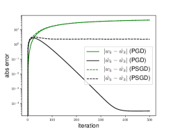
Refer to caption Refer to caption Refer to caption
(a) GD and SGD (b) PGD and PSGD (c) NGD and PNGD
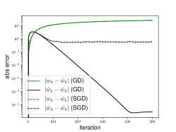
Figure 4: Linear regression on MNIST dataset. X-axis: iteration; y-axis: the absolute approximation error in logarithmic scale. Green lines represent wtw^t1subscriptnormsubscript𝑤𝑡subscript^𝑤𝑡1\left\|{w}_{t}-\hat{w}_{t}\right\|_{1} and black lines represent w~tw^t1subscriptnormsubscript~𝑤𝑡subscript^𝑤𝑡1\left\|\tilde{w}_{t}-\hat{w}_{t}\right\|_{1}, where wtsubscript𝑤𝑡w_{t}, w^tsubscript^𝑤𝑡\hat{w}_{t} and w~tsubscript~𝑤𝑡\tilde{w}_{t} are the unregularized path, the regularized path and the iterate averaged path, respectively. Solid lines and dashed lines are the results obtained by running deterministic and stochastic algorithms respectively. For deterministic algorithms, the error between w~tsubscript~𝑤𝑡\tilde{w}_{t} and w^tsubscript^𝑤𝑡\hat{w}_{t} converges to zero. For stochastic algorithms, the error between w~tsubscript~𝑤𝑡\tilde{w}_{t} and w^tsubscript^𝑤𝑡\hat{w}_{t} remains small.

Linear regression

Firstly, we study linear regression under quadratic loss functions and the regularization effects caused by averaging the optimization paths of (S)GD, P(S)GD and N(S)GD. The learning rates are set to be constant. For P(S)GD, we set the preconditioning matrix as the Hessian, which is known as the Newton’s method.

Our theories predict that averaging the (S)GD and N(S)GD paths leads to the solutions biased by 2subscript2\ell_{2}-regularizers (Theorem 13), while averaging the P(S)GD path introduces an effect of the generalized 2subscript2\ell_{2}-regularization (Theorem 2). To verify the predictions, we generate the paths of the averaged solutions w~ksubscript~𝑤𝑘\tilde{w}_{k} and the regularized solutions w^ksubscript^𝑤𝑘\hat{w}_{k}, and then compute the approximation errors between them. The results are plotted in Figure 4.

In Figure 4 (a), the solid lines clearly indicate that the averaged solution converges to the regularized solution when running GD, which also corresponds to the convergence in expectation in SGD cases, as predicted by Theorem 1. For SGD, however, the dashed lines in Figure 4 (a) show that there is a small error between the averaged solution and the regularized solution. The error exists since the convergence of the averaged solution does not hold in probability. Luckily, the error would not grow large as the deviation of the averaged solution is controllable by Theorem 1. Hence by comparing the dashed green and black lines, we see that averaging the SGD path still leads to an effect of 2subscript2\ell_{2}-regularization ignoring a tolerable error.

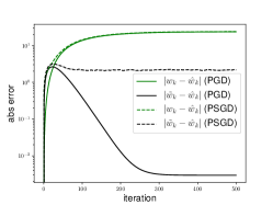
Figure 4 (b) shows the results for PGD and PSGD. Again, averaging the PGD path causes a perfect generalized 2subscript2\ell_{2}-regularization effect, and there is a small gap for averaging the optimization path with noise. These support Theorem 2.

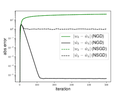
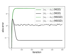
The results related to NGD and NSGD are shown in Figure 4 (c). Again, for the deterministic algorithm, the solid lines manifest the convergence between the averaged solution and the regularized solution, verifying our Theorem 3. And the dashed lines once more suggest the stochastic algorithm causes a tolerable approximation error.
Refer to caption Refer to caption Refer to caption
(a) GD and SGD (b) PGD and PSGD (c) NGD and NSGD
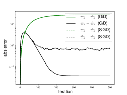
Figure 5: Logistic regression on MNIST dataset. X-axis: iteration; y-axis: the absolute approximation error in logarithmic scale. Green lines represent wtw^t1subscriptnormsubscript𝑤𝑡subscript^𝑤𝑡1\left\|{w}_{t}-\hat{w}_{t}\right\|_{1} and black lines represent w~tw^t1subscriptnormsubscript~𝑤𝑡subscript^𝑤𝑡1\left\|\tilde{w}_{t}-\hat{w}_{t}\right\|_{1}, where wtsubscript𝑤𝑡w_{t}, w^tsubscript^𝑤𝑡\hat{w}_{t} and w~tsubscript~𝑤𝑡\tilde{w}_{t} are the unregularized path, the regularized path and the iterate averaged path, respectively. Solid lines and dashed lines are the results obtained by running deterministic and stochastic algorithms respectively. For both deterministic and stochastic algorithms, we see that the error between w~tsubscript~𝑤𝑡\tilde{w}_{t} and w^tsubscript^𝑤𝑡\hat{w}_{t} has a small upper bound. Moreover, the error bounds for the paths generated by stochastic algorithms are relatively bigger.

Logistic regression

Next we set the loss function L(w)𝐿𝑤L(w) to be the logistic regression objective with a small 2subscript2\ell_{2}-regularizer, which is then strongly convex and smooth, as required by Theorem 4. We firstly generate the unregularized paths and perform iterate averaging over them. Next, since it is impossible to visualize a high dimensional cubic with vertices decided by Theorem 4, instead we set λ=1/γ1/η𝜆1𝛾1𝜂\lambda={1}/{\gamma}-{1}/{\eta}, and add an extra regularization term with this particular hyperparameter to obtain the regularized paths. Lastly we measure the errors between the averaged solutions and the regularized solutions to verify the effect of iterate averaging applied on strongly convex and smooth loss functions. The learning rates are set to be constant. The approximation errors are plotted in Figure 5.

In Figure 5 (a), the solid black line measures the error between the averaged GD path and the regularized GD path, and indeed the error is bounded and small as predicted by Theorem 4; the dashed black line is the result obtained by running SGD, which suggests that the approximation error, though increases a little due to randomness, is still small.

For completeness, we also test P(S)GD and N(S)GD with results shown in Figure 5 (b) and (c). For P(S)GD, we use the Hessian in linear regression experiments as the preconditioning matrix (since the Hessian of the logistic loss varies during training). Figure 5 (b) and (c) show that the averaged solutions approximately achieve the generalized/vanilla 2subscript2\ell_{2}-regularization effects respectively. And for the stochastic optimization paths, the approximation errors between the averaged paths and the regularized paths increase by a small amount due to the randomness of the algorithms.

4.3 Application in deep neural networks

Lastly, we study the benefits of using iterate averaging in modern deep neural networks.

We train VGG-16 (Simonyan & Zisserman, 2014) and ResNet-18 (He et al., 2016) on CIFAR-10 and CIFAR-100 datasets, with standard tricks including batch normalization, data augmentation, learning rate decay and weight decay. All experiments are repeated three times to obtain the mean and deviation. The running times are measured by performing the experiments using a single GPU K80. The models are trained for 300300300 epochs using SGD. We perform “epoch averaging” using the 240240240 checkpoints saved from the 616161st to the 300300300th epoch. The first 606060 epochs are skipped since the models in the early phase are extremely unstable. After averaging the parameters, we apply a trick proposed by Izmailov et al. (2018) to handle the batch normalization statistics which are not trained by SGD. Specifically, we make a forward pass on the training data to compute the activation statistics for the batch normalization layers. For the choice of averaging scheme, we test standard geometric distribution with success probability p{0.9999,0.999,0.99,0.9}𝑝0.99990.9990.990.9p\in\{0.9999,0.999,0.99,0.9\}.

Table 1: CIFAR-10 and CIFAR-100 experiments
Dataset CIFAR-10 CIFAR-100
Model VGG-16 ResNet-18 ResNet-18
Accuracy after training (%percent\%) 92.5492.5492.54 ±0.22plus-or-minus0.22\pm 0.22 94.5494.5494.54 ±0.04plus-or-minus0.04\pm 0.04 75.6275.6275.62 ±0.16plus-or-minus0.16\pm 0.16
Accuracy after averaging (%percent\%) 93.1893.18\bm{93.18} ±0.06plus-or-minus0.06\pm 0.06 94.7294.72\bm{94.72} ±0.04plus-or-minus0.04\pm 0.04 76.2476.24\bm{76.24} ±0.05plus-or-minus0.05\pm 0.05
Time of training 4.5similar-toabsent4.5\sim 4.5h 8.3similar-toabsent8.3\sim 8.3h 8.3similar-toabsent8.3\sim 8.3h
Time of averaging333The time of averaging contains the time of IO and fixing BN, which takes the major overhead. For example, in CIFAR-10 and VGG-16 experiments, IO takes 22similar-toabsent22\sim 22s, fixing BN takes 18similar-toabsent18\sim 18s, while performing averaging and evaluation take merely 7similar-toabsent7\sim 7s. 47similar-toabsent47\sim 47s 56similar-toabsent56\sim 56s 58similar-toabsent58\sim 58s

The results are shown in Table 1. We see that (i) averaging the SGD path does improve performance since it introduce an implicit regularization by our understanding; (ii) obtaining such regularization by iterate averaging is computationally cheap. It only takes a few seconds to test a hyperparameter of the averaging scheme. In contrast, several hours are required to test a hyperparameter for traditional explicit regularization since it requires re-training the model. Finally, we emphasize that the space cost of our method is also affordable. In fact, in our experiments, we perform epoch-wise averaging instead of iterate-wise averaging, thus we only need to store a few hundreds of the checkpoints.

5 Discussion

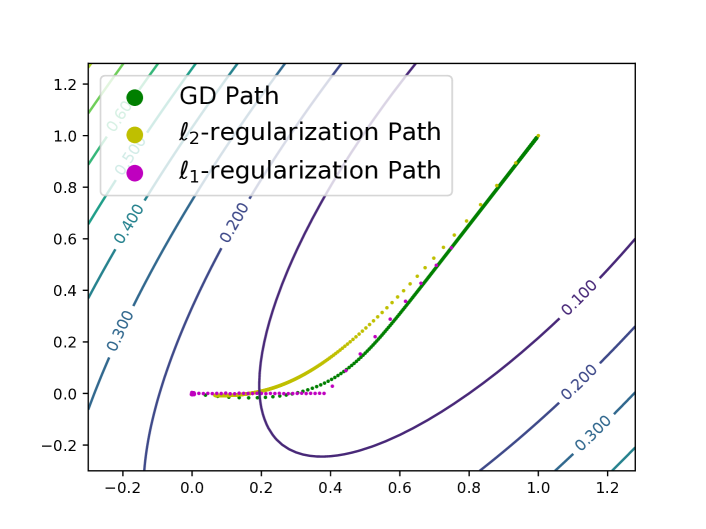
1subscript1\ell_{1}-regularization

Notice that all our results obtain 2subscript2\ell_{2}-type regularization effects. A natural follow-up question would be whether or not there is an averaging scheme that acts as an 1subscript1\ell_{1}-regularizer. However, we here provide some evidence that this question is relatively hard. As illustrated in Figure 6, even for simple quadratic loss, the 1subscript1\ell_{1}-regularized solutions could lie outside of the convex hull of a SGD path. Therefore, any averaging scheme with positive weights fails to obtain such 1subscript1\ell_{1}-regularized solutions.

Refer to caption
Figure 6: A 2-D demonstration of the 1subscript1\ell_{1}-regularization path. Green dots: the vanilla GD path wtsubscript𝑤𝑡w_{t}; yellow dots: the 2subscript2\ell_{2}-regularization path w^λ,2subscript^𝑤𝜆subscript2\hat{w}_{{\lambda},\ell_{2}}; purple dots: the 1subscript1\ell_{1}-regularization path w^λ,1subscript^𝑤𝜆subscript1\hat{w}_{{\lambda},\ell_{1}}. There exist 1subscript1\ell_{1}-regularized solutions outside of the convex hull of the GD path, while all of the 2subscript2\ell_{2}-regularized solutions are inside of that.

Infinite width neural network

Recent works suggest that a sufficient wide neural network trained by SGD behaves like a quadratic model, i.e., the neural tangent kernel (NTK) (Jacot et al., 2018; Arora et al., 2019; Cao & Gu, 2019). Nonetheless, the NTK approximation fails when there is an explicit 2subscript2\ell_{2}-regularizer (Wei et al., 2019). Since our results hold for kernel ridge regression, we conjecture that iterate averaging could be a potential approach to achieve 2subscript2\ell_{2}-regularization for the NTK regime. We leave further investigation of this issue in future works.

6 Conclusions

In this work, we establish averaging schemes for various optimization methods and objective functions to obtain adjustable 2subscript2\ell_{2}-type regularization effects, i.e., SGD with preconditioning and adaptive learning rate schedules, Nesterov’s accelerated stochastic gradient descent, and strongly convex and smooth objective functions. Particularly, we resolve an open question in (Neu & Rosasco, 2018). The method of achieving regularization by iterate averaging requires little computation. It is further shown experimentally that iterate averaging even benefits practical deep learning models. Our theoretical and empirical results demonstrate the potential of adopting iterate averaging to obtain adjustable regularization for free in a much broader class of optimization methods and objective functions.

Acknowledgement

This research is supported in part by NSF CAREER grant 1652257, ONR Award N00014-18-1-2364 and the Lifelong Learning Machines program from DARPA/MTO.

References

  • Arora et al. (2019) Arora, S., Du, S. S., Hu, W., Li, Z., Salakhutdinov, R., and Wang, R. On exact computation with an infinitely wide neural net. arXiv preprint arXiv:1904.11955, 2019.
  • Bach & Moulines (2013) Bach, F. and Moulines, E. Non-strongly-convex smooth stochastic approximation with convergence rate o (1/n). In Advances in neural information processing systems, pp. 773–781, 2013.
  • Beck & Teboulle (2009) Beck, A. and Teboulle, M. A fast iterative shrinkage-thresholding algorithm for linear inverse problems. SIAM journal on imaging sciences, 2(1):183–202, 2009.
  • Bottou & Bousquet (2008) Bottou, L. and Bousquet, O. The tradeoffs of large scale learning. In Advances in neural information processing systems, pp. 161–168, 2008.
  • Cai et al. (2018) Cai, Y., Li, Q., and Shen, Z. A quantitative analysis of the effect of batch normalization on gradient descent. arXiv preprint arXiv:1810.00122, 2018.
  • Cao & Gu (2019) Cao, Y. and Gu, Q. Generalization bounds of stochastic gradient descent for wide and deep neural networks. arXiv preprint arXiv:1905.13210, 2019.
  • Clark (1987) Clark, D. S. Short proof of a discrete gronwall inequality. Discrete applied mathematics, 16(3):279–281, 1987.
  • Dennis Jr & Schnabel (1996) Dennis Jr, J. E. and Schnabel, R. B. Numerical methods for unconstrained optimization and nonlinear equations, volume 16. Siam, 1996.
  • Devlin et al. (2018) Devlin, J., Chang, M.-W., Lee, K., and Toutanova, K. Bert: Pre-training of deep bidirectional transformers for language understanding. arXiv preprint arXiv:1810.04805, 2018.
  • Grandvalet & Bengio (2005) Grandvalet, Y. and Bengio, Y. Semi-supervised learning by entropy minimization. In Advances in neural information processing systems, pp. 529–536, 2005.
  • Granziol et al. (2020) Granziol, D., Wan, X., and Roberts, S. Iterate averaging helps: An alternative perspective in deep learning. arXiv preprint arXiv:2003.01247, 2020.
  • Gunasekar et al. (2018) Gunasekar, S., Lee, J., Soudry, D., and Srebro, N. Characterizing implicit bias in terms of optimization geometry. arXiv preprint arXiv:1802.08246, 2018.
  • He et al. (2015) He, K., Zhang, X., Ren, S., and Sun, J. Delving deep into rectifiers: Surpassing human-level performance on imagenet classification. In Proceedings of the IEEE international conference on computer vision, pp.  1026–1034, 2015.
  • He et al. (2016) He, K., Zhang, X., Ren, S., and Sun, J. Deep residual learning for image recognition. 2016 IEEE Conference on Computer Vision and Pattern Recognition (CVPR), Jun 2016. doi: 10.1109/cvpr.2016.90. URL http://dx.doi.org/10.1109/CVPR.2016.90.
  • Hu et al. (2017a) Hu, W., Li, C. J., Li, L., and Liu, J.-G. On the diffusion approximation of nonconvex stochastic gradient descent. arXiv preprint arXiv:1705.07562, 2017a.
  • Hu et al. (2017b) Hu, W., Li, C. J., and Su, W. On the global convergence of a randomly perturbed dissipative nonlinear oscillator. arXiv preprint arXiv:1712.05733, 2017b.
  • Hu et al. (2020) Hu, W., Xiao, L., and Pennington, J. Provable benefit of orthogonal initialization in optimizing deep linear networks. arXiv preprint arXiv:2001.05992, 2020.
  • Ioffe & Szegedy (2015) Ioffe, S. and Szegedy, C. Batch normalization: Accelerating deep network training by reducing internal covariate shift. arXiv preprint arXiv:1502.03167, 2015.
  • Izmailov et al. (2018) Izmailov, P., Podoprikhin, D., Garipov, T., Vetrov, D., and Wilson, A. G. Averaging weights leads to wider optima and better generalization. arXiv preprint arXiv:1803.05407, 2018.
  • Jacot et al. (2018) Jacot, A., Gabriel, F., and Hongler, C. Neural tangent kernel: Convergence and generalization in neural networks. In Advances in neural information processing systems, pp. 8571–8580, 2018.
  • Jain et al. (2018) Jain, P., Kakade, S., Kidambi, R., Netrapalli, P., and Sidford, A. Parallelizing stochastic gradient descent for least squares regression: mini-batching, averaging, and model misspecification. Journal of Machine Learning Research, 18, 2018.
  • Krogh & Hertz (1992) Krogh, A. and Hertz, J. A. A simple weight decay can improve generalization. In Advances in neural information processing systems, pp. 950–957, 1992.
  • Lakshminarayanan & Szepesvari (2018) Lakshminarayanan, C. and Szepesvari, C. Linear stochastic approximation: How far does constant step-size and iterate averaging go? In International Conference on Artificial Intelligence and Statistics, pp.  1347–1355, 2018.
  • Li et al. (2017) Li, Q., Tai, C., et al. Stochastic modified equations and adaptive stochastic gradient algorithms. In Proceedings of the 34th International Conference on Machine Learning-Volume 70, pp.  2101–2110. JMLR. org, 2017.
  • Martens (2014) Martens, J. New insights and perspectives on the natural gradient method. arXiv preprint arXiv:1412.1193, 2014.
  • Mohri et al. (2018) Mohri, M., Rostamizadeh, A., and Talwalkar, A. Foundations of machine learning. MIT press, 2018.
  • Nesterov (1983) Nesterov, Y. E. A method for solving the convex programming problem with convergence rate o (1/k^ 2). In Dokl. akad. nauk Sssr, volume 269, pp.  543–547, 1983.
  • Neu & Rosasco (2018) Neu, G. and Rosasco, L. Iterate averaging as regularization for stochastic gradient descent. arXiv preprint arXiv:1802.08009, 2018.
  • Shi et al. (2019) Shi, B., Du, S. S., Su, W., and Jordan, M. I. Acceleration via symplectic discretization of high-resolution differential equations. In Advances in Neural Information Processing Systems, pp. 5745–5753, 2019.
  • Silver et al. (2017) Silver, D., Schrittwieser, J., Simonyan, K., Antonoglou, I., Huang, A., Guez, A., Hubert, T., Baker, L., Lai, M., Bolton, A., et al. Mastering the game of go without human knowledge. Nature, 550(7676):354, 2017.
  • Simonyan & Zisserman (2014) Simonyan, K. and Zisserman, A. Very deep convolutional networks for large-scale image recognition. arXiv preprint arXiv:1409.1556, 2014.
  • Soudry et al. (2018) Soudry, D., Hoffer, E., Nacson, M. S., Gunasekar, S., and Srebro, N. The implicit bias of gradient descent on separable data. The Journal of Machine Learning Research, 19(1):2822–2878, 2018.
  • Su et al. (2014) Su, W., Boyd, S., and Candes, E. A differential equation for modeling nesterov’s accelerated gradient method: Theory and insights. In Advances in Neural Information Processing Systems, pp. 2510–2518, 2014.
  • Suggala et al. (2018) Suggala, A., Prasad, A., and Ravikumar, P. K. Connecting optimization and regularization paths. In Advances in Neural Information Processing Systems, pp. 10608–10619, 2018.
  • Tibshirani (1996) Tibshirani, R. Regression shrinkage and selection via the lasso. Journal of the Royal Statistical Society: Series B (Methodological), 58(1):267–288, 1996.
  • Tikhonov & Arsenin (1977) Tikhonov, A. N. and Arsenin, V. Y. Solutions of ill-posed problems. V. H. Winston & Sons, Washington, D.C.: John Wiley & Sons, New York, 1977. Translated from the Russian, Preface by translation editor Fritz John, Scripta Series in Mathematics.
  • Wei et al. (2019) Wei, C., Lee, J. D., Liu, Q., and Ma, T. Regularization matters: Generalization and optimization of neural nets vs their induced kernel. In Advances in Neural Information Processing Systems, pp. 9709–9721, 2019.
  • Wilson et al. (2017) Wilson, A. C., Roelofs, R., Stern, M., Srebro, N., and Recht, B. The marginal value of adaptive gradient methods in machine learning. In Advances in Neural Information Processing Systems, pp. 4148–4158, 2017.
  • Yang et al. (2018) Yang, L., Arora, R., Zhao, T., et al. The physical systems behind optimization algorithms. In Advances in Neural Information Processing Systems, pp. 4372–4381, 2018.
  • Zhang et al. (2016) Zhang, C., Bengio, S., Hardt, M., Recht, B., and Vinyals, O. Understanding deep learning requires rethinking generalization. arXiv preprint arXiv:1611.03530, 2016.
  • Zhang et al. (2019) Zhang, M., Lucas, J., Ba, J., and Hinton, G. E. Lookahead optimizer: k steps forward, 1 step back. In Advances in Neural Information Processing Systems, pp. 9593–9604, 2019.
  • Zhou (2018) Zhou, X. On the fenchel duality between strong convexity and lipschitz continuous gradient. arXiv preprint arXiv:1803.06573, 2018.
  • Zhu et al. (2018) Zhu, Z., Wu, J., Yu, B., Wu, L., and Ma, J. The anisotropic noise in stochastic gradient descent: Its behavior of escaping from minima and regularization effects. arXiv preprint arXiv:1803.00195, 2018.

Appendix A Continuous analysis

To motivate our proofs for the theorems in main text, let us first elaborate the continuous cases. Then we will extend our analysis to the discrete circumstances. One can safely skip this part and go directly to Section C for the missing proofs in main text, which is self-consistent.

Continuous optimization paths

To ease notations and preliminaries, in this part we only discuss gradient descent (GD) and Nesterov’s accelerated gradient descent (NGD), and their strong continuous approximation via ordinary differential equations (ODEs). For SGD and NSGD, existing works show that there are weak continuous approximation by stochastic differential equations (SDEs) (Hu et al., 2017a, b; Li et al., 2017). Our analysis can be extended to SDEs, but we believe it serves better to motivate our discrete proofs by focusing on ODEs.

We consider loss L(w)𝐿𝑤L(w) and 2subscript2\ell_{2}-regularizer R(w)=12w22𝑅𝑤12superscriptsubscriptnorm𝑤22R(w)=\frac{1}{2}\left\|w\right\|_{2}^{2}. Let the learning rate η0𝜂0\eta\to 0, the path of L(w)𝐿𝑤L(w) optimized by GD converges to the following ODE (Yang et al., 2018)

dwt=L(wt)dt.dsubscript𝑤𝑡𝐿subscript𝑤𝑡d𝑡\mathrm{d}w_{t}=-\operatorname{\nabla}L(w_{t})\mathrm{d}t.

Similarly the continuous GD optimization path of regularized loss admits

dw^t=(L(w^t)+λw^t)dt.dsubscript^𝑤𝑡𝐿subscript^𝑤𝑡𝜆subscript^𝑤𝑡d𝑡\mathrm{d}\hat{w}_{t}=-\left(\operatorname{\nabla}L(\hat{w}_{t})+\lambda\hat{w}_{t}\right)\mathrm{d}t.

As for NGD, Su et al. (2014); Yang et al. (2018) show if the loss is α𝛼\alpha-strongly convex, then the NGD optimization path converges to

wt′′+2αwt+L(wt)=0.subscriptsuperscript𝑤′′𝑡2𝛼subscriptsuperscript𝑤𝑡superscript𝐿subscript𝑤𝑡0w^{\prime\prime}_{t}+2\sqrt{\alpha}w^{\prime}_{t}+L^{\prime}(w_{t})=0.

Since L^(w^)=L(w^)+λ2w^22^𝐿^𝑤𝐿^𝑤𝜆2superscriptsubscriptnorm^𝑤22\hat{L}(\hat{w})=L(\hat{w})+\frac{\lambda}{2}\left\|\hat{w}\right\|_{2}^{2} is (α+λ)𝛼𝜆(\alpha+\lambda)-strongly convex, the NGD path of the regularized loss satisfies

w^t′′+2α+λw^t+L(w^t)+λw^t=0.subscriptsuperscript^𝑤′′𝑡2𝛼𝜆subscriptsuperscript^𝑤𝑡superscript𝐿subscript^𝑤𝑡𝜆subscript^𝑤𝑡0\hat{w}^{\prime\prime}_{t}+2\sqrt{\alpha+\lambda}\hat{w}^{\prime}_{t}+L^{\prime}(\hat{w}_{t})+\lambda\hat{w}_{t}=0.

Continuous weighting scheme

We define the continuous weighting scheme as

pt0,t0,Pt=0tp(s)ds,limtPt=1.formulae-sequencesubscript𝑝𝑡0formulae-sequence𝑡0formulae-sequencesubscript𝑃𝑡superscriptsubscript0𝑡𝑝𝑠differential-d𝑠subscript𝑡subscript𝑃𝑡1p_{t}\geq 0,\quad t\geq 0,\quad P_{t}=\int_{0}^{t}p(s)\mathrm{d}s,\quad\lim_{t\to\infty}P_{t}=1.
Lemma 1.

Given two continuous dynamic xt,x^t,t0subscript𝑥𝑡subscript^𝑥𝑡𝑡0x_{t},\ \hat{x}_{t},\ t\geq 0. Let x~t=Pt10tpsxsdssubscript~𝑥𝑡superscriptsubscript𝑃𝑡1superscriptsubscript0𝑡subscript𝑝𝑠subscript𝑥𝑠differential-d𝑠\tilde{x}_{t}=P_{t}^{-1}\int_{0}^{t}p_{s}x_{s}\mathrm{d}s. Suppose x0=x^0=0subscript𝑥0subscript^𝑥00x_{0}=\hat{x}_{0}=0. If the continuous weighting scheme Ptsubscript𝑃𝑡P_{t} satisfies

dx^t=(1Pt)dxt,t0,formulae-sequencedsubscript^𝑥𝑡1subscript𝑃𝑡dsubscript𝑥𝑡𝑡0\mathrm{d}\hat{x}_{t}=(1-P_{t})\mathrm{d}x_{t},\quad t\geq 0,

then we have

Pt(xtx~t)=xtx^t,t0,formulae-sequencesubscript𝑃𝑡subscript𝑥𝑡subscript~𝑥𝑡subscript𝑥𝑡subscript^𝑥𝑡𝑡0P_{t}(x_{t}-\tilde{x}_{t})=x_{t}-\hat{x}_{t},\quad t\geq 0,

and

x^tx~t=(1Pt)(xtx~t),t0.formulae-sequencesubscript^𝑥𝑡subscript~𝑥𝑡1subscript𝑃𝑡subscript𝑥𝑡subscript~𝑥𝑡𝑡0\hat{x}_{t}-\tilde{x}_{t}=(1-P_{t})(x_{t}-\tilde{x}_{t}),\quad t\geq 0.
Proof.

By definition we have for t0𝑡0t\geq 0,

x~t=Pt10tpsxsds=Pt1(xsPs|0t0tPsdxs)=xtPt10tPsdxssubscript~𝑥𝑡superscriptsubscript𝑃𝑡1superscriptsubscript0𝑡subscript𝑝𝑠subscript𝑥𝑠differential-d𝑠superscriptsubscript𝑃𝑡1evaluated-atsubscript𝑥𝑠subscript𝑃𝑠0𝑡superscriptsubscript0𝑡subscript𝑃𝑠differential-dsubscript𝑥𝑠subscript𝑥𝑡superscriptsubscript𝑃𝑡1superscriptsubscript0𝑡subscript𝑃𝑠differential-dsubscript𝑥𝑠\displaystyle\tilde{x}_{t}=P_{t}^{-1}\int_{0}^{t}p_{s}x_{s}\mathrm{d}s=P_{t}^{-1}\left(\left.x_{s}P_{s}\right|_{0}^{t}-\int_{0}^{t}P_{s}\mathrm{d}x_{s}\right)=x_{t}-P_{t}^{-1}\int_{0}^{t}P_{s}\mathrm{d}x_{s}
=\displaystyle= xtPt1(xt0t(1Ps)dxs)=xtPt1(xt0tdx^s)subscript𝑥𝑡superscriptsubscript𝑃𝑡1subscript𝑥𝑡superscriptsubscript0𝑡1subscript𝑃𝑠differential-dsubscript𝑥𝑠subscript𝑥𝑡superscriptsubscript𝑃𝑡1subscript𝑥𝑡superscriptsubscript0𝑡differential-dsubscript^𝑥𝑠\displaystyle x_{t}-P_{t}^{-1}\left(x_{t}-\int_{0}^{t}(1-P_{s})\mathrm{d}x_{s}\right)=x_{t}-P_{t}^{-1}\left(x_{t}-\int_{0}^{t}\mathrm{d}\hat{x}_{s}\right)
=\displaystyle= xtPt1(xtx^t).subscript𝑥𝑡superscriptsubscript𝑃𝑡1subscript𝑥𝑡subscript^𝑥𝑡\displaystyle x_{t}-P_{t}^{-1}\left(x_{t}-\hat{x}_{t}\right).

Thus

Pt(xtx~t)=xtx^t,subscript𝑃𝑡subscript𝑥𝑡subscript~𝑥𝑡subscript𝑥𝑡subscript^𝑥𝑡P_{t}(x_{t}-\tilde{x}_{t})=x_{t}-\hat{x}_{t},

and

x^tx~t=xtPt(xtx~t)x~t=(1Pt)(xtx~t).subscript^𝑥𝑡subscript~𝑥𝑡subscript𝑥𝑡subscript𝑃𝑡subscript𝑥𝑡subscript~𝑥𝑡subscript~𝑥𝑡1subscript𝑃𝑡subscript𝑥𝑡subscript~𝑥𝑡\hat{x}_{t}-\tilde{x}_{t}=x_{t}-P_{t}(x_{t}-\tilde{x}_{t})-\tilde{x}_{t}=(1-P_{t})(x_{t}-\tilde{x}_{t}).

A.1 Continuous Theorem 1

Consider linear regression problem L(w)=12ni=1nwxiyi22=12wΣwwa+const𝐿𝑤12𝑛superscriptsubscript𝑖1𝑛superscriptsubscriptnormsuperscript𝑤topsubscript𝑥𝑖subscript𝑦𝑖2212superscript𝑤topΣ𝑤superscript𝑤top𝑎constL(w)=\frac{1}{2n}\sum_{i=1}^{n}\left\|w^{\top}x_{i}-y_{i}\right\|_{2}^{2}=\frac{1}{2}w^{\top}\Sigma w-w^{\top}a+\text{const}, and 2subscript2\ell_{2}-regularizer R(w)=12w22𝑅𝑤12superscriptsubscriptnorm𝑤22R(w)=\frac{1}{2}\left\|w\right\|_{2}^{2}. Assume the initial condition w0=w^0=0subscript𝑤0subscript^𝑤00w_{0}=\hat{w}_{0}=0, then the GD dynamics for the unregularized and regularized losses are

dwt=(Σwta)dt,w0=0,formulae-sequencedsubscript𝑤𝑡Σsubscript𝑤𝑡𝑎d𝑡subscript𝑤00\displaystyle\mathrm{d}w_{t}=-\left(\Sigma w_{t}-a\right)\mathrm{d}t,\quad w_{0}=0,
dw^t=(Σw^ta+λw^t)dt,w^0=0.formulae-sequencedsubscript^𝑤𝑡Σsubscript^𝑤𝑡𝑎𝜆subscript^𝑤𝑡d𝑡subscript^𝑤00\displaystyle\mathrm{d}\hat{w}_{t}=-\left(\Sigma\hat{w}_{t}-a+\lambda\hat{w}_{t}\right)\mathrm{d}t,\quad\hat{w}_{0}=0.

The ODEs are solved by

wt=(IeΣt)Σ1a,w^t=(Ie(Σ+λI)t)(Σ+λI)1a.formulae-sequencesubscript𝑤𝑡𝐼superscript𝑒Σ𝑡superscriptΣ1𝑎subscript^𝑤𝑡𝐼superscript𝑒Σ𝜆𝐼𝑡superscriptΣ𝜆𝐼1𝑎w_{t}=\left(I-e^{-\Sigma t}\right)\Sigma^{-1}a,\quad\hat{w}_{t}=\left(I-e^{-(\Sigma+\lambda I)t}\right){\left(\Sigma+\lambda I\right)^{-1}}a.

Now let the continuous weighting scheme be

Pt=1eλt,subscript𝑃𝑡1superscript𝑒𝜆𝑡P_{t}=1-e^{\lambda t},

then we have

dw^t=(1Pt)dwt,dsubscript^𝑤𝑡1subscript𝑃𝑡dsubscript𝑤𝑡\mathrm{d}\hat{w}_{t}=(1-P_{t})\mathrm{d}w_{t},

thus by Lemma 1 we obtain

w^tw~t=(1Pt)(wtw~t),subscript^𝑤𝑡subscript~𝑤𝑡1subscript𝑃𝑡subscript𝑤𝑡subscript~𝑤𝑡\hat{w}_{t}-\tilde{w}_{t}=(1-P_{t})(w_{t}-\tilde{w}_{t}),

which proves the continuous version of Theorem 1.

A.2 Continuous Theorem 3

Consider linear regression problem L(w)=12ni=1nwxiyi22=12wΣwwa+const𝐿𝑤12𝑛superscriptsubscript𝑖1𝑛superscriptsubscriptnormsuperscript𝑤topsubscript𝑥𝑖subscript𝑦𝑖2212superscript𝑤topΣ𝑤superscript𝑤top𝑎constL(w)=\frac{1}{2n}\sum_{i=1}^{n}\left\|w^{\top}x_{i}-y_{i}\right\|_{2}^{2}=\frac{1}{2}w^{\top}\Sigma w-w^{\top}a+\text{const}, and 2subscript2\ell_{2}-regularizer R(w)=12w22𝑅𝑤12superscriptsubscriptnorm𝑤22R(w)=\frac{1}{2}\left\|w\right\|_{2}^{2}. Assume the initial condition w0=w0=0subscript𝑤0subscriptsuperscript𝑤00w_{0}=w^{\prime}_{0}=0 and w^0=w^0=0subscript^𝑤0subscriptsuperscript^𝑤00\hat{w}_{0}=\hat{w}^{\prime}_{0}=0. Then the unregularized and regularized NGD dynamics are

wt′′+2αwt+Σwta=0,w0=w0=0,formulae-sequencesubscriptsuperscript𝑤′′𝑡2𝛼subscriptsuperscript𝑤𝑡Σsubscript𝑤𝑡𝑎0subscript𝑤0subscriptsuperscript𝑤00\displaystyle w^{\prime\prime}_{t}+2\sqrt{\alpha}w^{\prime}_{t}+\Sigma w_{t}-a=0,\quad w_{0}=w^{\prime}_{0}=0, (7)
w^t′′+2α+λw^t+(Σ+λ)w^ta=0,w^0=w^0=0.formulae-sequencesubscriptsuperscript^𝑤′′𝑡2𝛼𝜆subscriptsuperscript^𝑤𝑡Σ𝜆subscript^𝑤𝑡𝑎0subscript^𝑤0subscriptsuperscript^𝑤00\displaystyle\hat{w}^{\prime\prime}_{t}+2\sqrt{\alpha+\lambda}\hat{w}^{\prime}_{t}+(\Sigma+\lambda)\hat{w}_{t}-a=0,\quad\hat{w}_{0}=\hat{w}^{\prime}_{0}=0. (8)

We first solve the order-2 ODE Eq. (7) in the canonical way, and then obtain the solution of Eq. (8) similarly. To do so, let’s firstly ignore the constant term and solve the homogenous ODE of Eq. (7), and obtain two general solutions of the homogenous equation as

wt,1=eαtcosΣαt,wt,2=eαtsinΣαt.formulae-sequencesubscript𝑤𝑡1superscript𝑒𝛼𝑡Σ𝛼𝑡subscript𝑤𝑡2superscript𝑒𝛼𝑡Σ𝛼𝑡w_{t,1}=e^{\sqrt{\alpha}t}\cos{\sqrt{\Sigma-\alpha}t},\quad w_{t,2}=e^{\sqrt{\alpha}t}\sin{\sqrt{\Sigma-\alpha}t}.

Then we guess a particular solution of Eq. (7) as wt,0=Σ1asubscript𝑤𝑡0superscriptΣ1𝑎w_{t,0}=\Sigma^{-1}a. Thus the general solution of ODE (7) can be decomposed as wt=λ1wt,1+λ2wt,2+wt,0subscript𝑤𝑡subscript𝜆1subscript𝑤𝑡1subscript𝜆2subscript𝑤𝑡2subscript𝑤𝑡0w_{t}=\lambda_{1}w_{t,1}+\lambda_{2}w_{t,2}+w_{t,0}. Consider the initial conditions w0=w0=0subscript𝑤0subscriptsuperscript𝑤00w_{0}=w^{\prime}_{0}=0, we obtain λ1=Σ1a,λ2=Σ1a(Σα)1αformulae-sequencesubscript𝜆1superscriptΣ1𝑎subscript𝜆2superscriptΣ1𝑎superscriptΣ𝛼1𝛼\lambda_{1}=-{\Sigma^{-1}}a,\ \lambda_{2}=-{\Sigma^{-1}}a\sqrt{{(\Sigma-\alpha)^{-1}}\alpha}. Thus the solution of Eq. (7) is

wtsubscript𝑤𝑡\displaystyle w_{t} =Σ1a(1eαtcosΣαtα(Σα)1eαtsinΣαt),absentsuperscriptΣ1𝑎1superscript𝑒𝛼𝑡Σ𝛼𝑡𝛼superscriptΣ𝛼1superscript𝑒𝛼𝑡Σ𝛼𝑡\displaystyle={\Sigma^{-1}}a\left(1-e^{-\sqrt{\alpha}t}\cos{\sqrt{\Sigma-\alpha}t}-\sqrt{\alpha{(\Sigma-\alpha)^{-1}}}e^{-\sqrt{\alpha}t}\sin{\sqrt{\Sigma-\alpha}t}\right), (9)
wtsubscriptsuperscript𝑤𝑡\displaystyle w^{\prime}_{t} =a(Σα)1eαtsinΣαt.absent𝑎superscriptΣ𝛼1superscript𝑒𝛼𝑡Σ𝛼𝑡\displaystyle=a\sqrt{{(\Sigma-\alpha)^{-1}}}e^{-\sqrt{\alpha}t}\sin{\sqrt{\Sigma-\alpha}t}.

Repeat these procedures, Eq. (9) is solved by

w^tsubscript^𝑤𝑡\displaystyle\hat{w}_{t} =(Σ+λ)1a(1eα+λtcosΣαt(α+λ)(Σα)1eα+λtsinΣαt),absentsuperscriptΣ𝜆1𝑎1superscript𝑒𝛼𝜆𝑡Σ𝛼𝑡𝛼𝜆superscriptΣ𝛼1superscript𝑒𝛼𝜆𝑡Σ𝛼𝑡\displaystyle={(\Sigma+\lambda)^{-1}}a\left(1-e^{-\sqrt{\alpha+\lambda}t}\cos{\sqrt{\Sigma-\alpha}t}-\sqrt{\left(\alpha+\lambda\right){(\Sigma-\alpha)^{-1}}}e^{-\sqrt{\alpha+\lambda}t}\sin{\sqrt{\Sigma-\alpha}t}\right), (10)
w^tsubscriptsuperscript^𝑤𝑡\displaystyle\hat{w}^{\prime}_{t} =a(Σα)1eα+λtsinΣαt.absent𝑎superscriptΣ𝛼1superscript𝑒𝛼𝜆𝑡Σ𝛼𝑡\displaystyle=a{\sqrt{{(\Sigma-\alpha)^{-1}}}}e^{-\sqrt{\alpha+\lambda}t}\sin{\sqrt{\Sigma-\alpha}t}.

Now let the continuous weighting scheme be

Pt=1e(α+λλ)t,subscript𝑃𝑡1superscript𝑒𝛼𝜆𝜆𝑡P_{t}=1-e^{-(\sqrt{\alpha+\lambda}-\sqrt{\lambda})t},

then we have

dw^t=(1Pt)dwt,dsubscript^𝑤𝑡1subscript𝑃𝑡dsubscript𝑤𝑡\mathrm{d}\hat{w}_{t}=(1-P_{t})\mathrm{d}w_{t},

thus by Lemma 1 we obtain

w^tw~t=(1Pt)(wtw~t),subscript^𝑤𝑡subscript~𝑤𝑡1subscript𝑃𝑡subscript𝑤𝑡subscript~𝑤𝑡\hat{w}_{t}-\tilde{w}_{t}=(1-P_{t})(w_{t}-\tilde{w}_{t}),

which proves the continuous version of Theorem 3.

A.3 Continuous Theorem 4

Consider an α𝛼\alpha-strongly convex and β𝛽\beta-smooth loss function L(w)𝐿𝑤L(w), and 2subscript2\ell_{2}-regularizer. Without loss of generality assume the minimum of L(w)𝐿𝑤L(w) satisfies w>w0=0subscript𝑤subscript𝑤00w_{*}>w_{0}=0. Then by Lemma 3 we have

αwbL(w)βwb,w(0,w),formulae-sequence𝛼𝑤𝑏𝐿𝑤𝛽𝑤𝑏for-all𝑤0subscript𝑤\alpha w-b\leq\operatorname{\nabla}L(w)\leq\beta w-b,\quad\forall w\in(0,w_{*}),

where b=L(0)𝑏𝐿0b=-\operatorname{\nabla}L(0), and “\leq” is defined entry-wisely. We study the continuous optimization paths caused by GD.

Consider the following three dynamics:

dwt=L(wt)dt,dut=(αutb)dt,dvt=(βvtb)dt,w0=u0=v0=0.formulae-sequencedsubscript𝑤𝑡𝐿subscript𝑤𝑡d𝑡formulae-sequencedsubscript𝑢𝑡𝛼subscript𝑢𝑡𝑏d𝑡formulae-sequencedsubscript𝑣𝑡𝛽subscript𝑣𝑡𝑏d𝑡subscript𝑤0subscript𝑢0subscript𝑣00\mathrm{d}w_{t}=-\operatorname{\nabla}L(w_{t})\mathrm{d}t,\quad\mathrm{d}u_{t}=-(\alpha u_{t}-b)\mathrm{d}t,\quad\mathrm{d}v_{t}=-(\beta v_{t}-b)\mathrm{d}t,\quad w_{0}=u_{0}=v_{0}=0.

By the comparison theorem of ODEs (Gronwall’s inequality), and solution of linear ODEs, we claim that for all t>0𝑡0t>0,

vtwtut,ut=bα(1eαt),vt=bβ(1eβt).formulae-sequencesubscript𝑣𝑡subscript𝑤𝑡subscript𝑢𝑡formulae-sequencesubscript𝑢𝑡𝑏𝛼1superscript𝑒𝛼𝑡subscript𝑣𝑡𝑏𝛽1superscript𝑒𝛽𝑡v_{t}\leq w_{t}\leq u_{t},\quad u_{t}=\frac{b}{\alpha}(1-e^{-\alpha t}),\quad v_{t}=\frac{b}{\beta}(1-e^{-\beta t}). (11)

In a similar manner, for the following three dynamics of regularized loss:

dw^t,λ=(L(w^t,λ)+λw^t,λ)dt,dsubscript^𝑤𝑡𝜆𝐿subscript^𝑤𝑡𝜆𝜆subscript^𝑤𝑡𝜆d𝑡\displaystyle\mathrm{d}\hat{w}_{t,\lambda}=-(\operatorname{\nabla}L(\hat{w}_{t,\lambda})+\lambda\hat{w}_{t,\lambda})\mathrm{d}t,\quad du^t,λ=((λ+α)u^t,λb)dt,dv^t,λ=((λ+β)v^t,λb)dt,formulae-sequencedsubscript^𝑢𝑡𝜆𝜆𝛼subscript^𝑢𝑡𝜆𝑏d𝑡dsubscript^𝑣𝑡𝜆𝜆𝛽subscript^𝑣𝑡𝜆𝑏d𝑡\displaystyle\mathrm{d}\hat{u}_{t,\lambda}=-((\lambda+\alpha)\hat{u}_{t,\lambda}-b)\mathrm{d}t,\quad\mathrm{d}\hat{v}_{t,\lambda}=-((\lambda+\beta)\hat{v}_{t,\lambda}-b)\mathrm{d}t,

where w^0,λ=u^0,λ=v^0,λ=0subscript^𝑤0𝜆subscript^𝑢0𝜆subscript^𝑣0𝜆0\hat{w}_{0,\lambda}=\hat{u}_{0,\lambda}=\hat{v}_{0,\lambda}=0. Similarly we have for all t>0𝑡0t>0,

v^t,λw^t,λu^t,λ,u^t,λ=bλ+α(1e(λ+α)t),v^t,λ=bλ+β(1e(λ+β)t).formulae-sequencesubscript^𝑣𝑡𝜆subscript^𝑤𝑡𝜆subscript^𝑢𝑡𝜆formulae-sequencesubscript^𝑢𝑡𝜆𝑏𝜆𝛼1superscript𝑒𝜆𝛼𝑡subscript^𝑣𝑡𝜆𝑏𝜆𝛽1superscript𝑒𝜆𝛽𝑡\hat{v}_{t,\lambda}\leq\hat{w}_{t,\lambda}\leq\hat{u}_{t,\lambda},\quad\hat{u}_{t,\lambda}=\frac{b}{\lambda+\alpha}(1-e^{-(\lambda+\alpha)t}),\quad\hat{v}_{t,\lambda}=\frac{b}{\lambda+\beta}(1-e^{-(\lambda+\beta)t}).

For the continuous weighting scheme

Pt=1eζt,pt=ζeζt,t0,ζ>0,formulae-sequencesubscript𝑃𝑡1superscript𝑒𝜁𝑡formulae-sequencesubscript𝑝𝑡𝜁superscript𝑒𝜁𝑡formulae-sequence𝑡0𝜁0P_{t}=1-e^{-\zeta t},\quad p_{t}=\zeta e^{-\zeta t},\quad t\geq 0,\quad\zeta>0,

the averaged solution is defined as w~t=Pt10tptwtdt=wtPt10tPsdwssubscript~𝑤𝑡superscriptsubscript𝑃𝑡1superscriptsubscript0𝑡subscript𝑝𝑡subscript𝑤𝑡differential-d𝑡subscript𝑤𝑡superscriptsubscript𝑃𝑡1superscriptsubscript0𝑡subscript𝑃𝑠differential-dsubscript𝑤𝑠\tilde{w}_{t}={P_{t}^{-1}}\int_{0}^{t}p_{t}w_{t}\mathrm{d}t=w_{t}-{P_{t}^{-1}}\int_{0}^{t}P_{s}\mathrm{d}w_{s}, similar there are u~t,v~tsubscript~𝑢𝑡subscript~𝑣𝑡\tilde{u}_{t},\tilde{v}_{t}. Thanks to Eq. (11) and ptsubscript𝑝𝑡p_{t} being non-negative, we have v~tw~tu~tsubscript~𝑣𝑡subscript~𝑤𝑡subscript~𝑢𝑡\tilde{v}_{t}\leq\tilde{w}_{t}\leq\tilde{u}_{t}. Let

λ1=ζ+βα,λ2=ζ+αβ,formulae-sequencesubscript𝜆1𝜁𝛽𝛼subscript𝜆2𝜁𝛼𝛽\lambda_{1}=\zeta+\beta-\alpha,\quad\lambda_{2}=\zeta+\alpha-\beta,

then

Pt(utu~t)=subscript𝑃𝑡subscript𝑢𝑡subscript~𝑢𝑡absent\displaystyle P_{t}(u_{t}-\tilde{u}_{t})= 0tPsdus=0t(1e(λ2+βα)s)beαsdt=b0teαse(β+λ2)sdssuperscriptsubscript0𝑡subscript𝑃𝑠differential-dsubscript𝑢𝑠superscriptsubscript0𝑡1superscript𝑒subscript𝜆2𝛽𝛼𝑠𝑏superscript𝑒𝛼𝑠differential-d𝑡𝑏superscriptsubscript0𝑡superscript𝑒𝛼𝑠superscript𝑒𝛽subscript𝜆2𝑠d𝑠\displaystyle\int_{0}^{t}P_{s}\mathrm{d}u_{s}=\int_{0}^{t}(1-e^{-(\lambda_{2}+\beta-\alpha)s})be^{-\alpha s}\mathrm{d}t=b\int_{0}^{t}e^{-\alpha s}-e^{-(\beta+\lambda_{2})s}\mathrm{d}s
=\displaystyle= b(1α(1eαt)1λ2+β(1e(λ2+β)t))=utv^t,λ2.𝑏1𝛼1superscript𝑒𝛼𝑡1subscript𝜆2𝛽1superscript𝑒subscript𝜆2𝛽𝑡subscript𝑢𝑡subscript^𝑣𝑡subscript𝜆2\displaystyle b\left(\frac{1}{\alpha}(1-e^{-\alpha t})-\frac{1}{\lambda_{2}+\beta}(1-e^{-(\lambda_{2}+\beta)t})\right)=u_{t}-\hat{v}_{t,\lambda_{2}}.

Thus

w~tw^t,λ2u~tv^t,λ2=u~tut+Pt(utu~t)=(1Pt)(u~tut).subscript~𝑤𝑡subscript^𝑤𝑡subscript𝜆2subscript~𝑢𝑡subscript^𝑣𝑡subscript𝜆2subscript~𝑢𝑡subscript𝑢𝑡subscript𝑃𝑡subscript𝑢𝑡subscript~𝑢𝑡1subscript𝑃𝑡subscript~𝑢𝑡subscript𝑢𝑡\tilde{w}_{t}-\hat{w}_{t,\lambda_{2}}\leq\tilde{u}_{t}-\hat{v}_{t,\lambda_{2}}=\tilde{u}_{t}-u_{t}+P_{t}(u_{t}-\tilde{u}_{t})=(1-P_{t})(\tilde{u}_{t}-u_{t}).

Similarly, since

Pt(vtv~t)=subscript𝑃𝑡subscript𝑣𝑡subscript~𝑣𝑡absent\displaystyle P_{t}(v_{t}-\tilde{v}_{t})= 0tPsdvs=0t(1e(λ1β+α)s)beβsdt=b0teβse(α+λ1)sdssuperscriptsubscript0𝑡subscript𝑃𝑠differential-dsubscript𝑣𝑠superscriptsubscript0𝑡1superscript𝑒subscript𝜆1𝛽𝛼𝑠𝑏superscript𝑒𝛽𝑠differential-d𝑡𝑏superscriptsubscript0𝑡superscript𝑒𝛽𝑠superscript𝑒𝛼subscript𝜆1𝑠d𝑠\displaystyle\int_{0}^{t}P_{s}\mathrm{d}v_{s}=\int_{0}^{t}(1-e^{-(\lambda_{1}-\beta+\alpha)s})be^{-\beta s}\mathrm{d}t=b\int_{0}^{t}e^{-\beta s}-e^{-(\alpha+\lambda_{1})s}\mathrm{d}s
=\displaystyle= b(1β(1eβt)1λ1+α(1e(λ1+α)t))=vtu^t,λ1,𝑏1𝛽1superscript𝑒𝛽𝑡1subscript𝜆1𝛼1superscript𝑒subscript𝜆1𝛼𝑡subscript𝑣𝑡subscript^𝑢𝑡subscript𝜆1\displaystyle b\left(\frac{1}{\beta}(1-e^{-\beta t})-\frac{1}{\lambda_{1}+\alpha}(1-e^{-(\lambda_{1}+\alpha)t})\right)=v_{t}-\hat{u}_{t,\lambda_{1}},

we can obtain a lower bound as

w~tw^t,λ1v~tu^t,λ1=v~tvt+Pt(vtv~t)=(1Pt)(v~tvt).subscript~𝑤𝑡subscript^𝑤𝑡subscript𝜆1subscript~𝑣𝑡subscript^𝑢𝑡subscript𝜆1subscript~𝑣𝑡subscript𝑣𝑡subscript𝑃𝑡subscript𝑣𝑡subscript~𝑣𝑡1subscript𝑃𝑡subscript~𝑣𝑡subscript𝑣𝑡\tilde{w}_{t}-\hat{w}_{t,\lambda_{1}}\geq\tilde{v}_{t}-\hat{u}_{t,\lambda_{1}}=\tilde{v}_{t}-v_{t}+P_{t}(v_{t}-\tilde{v}_{t})=(1-P_{t})(\tilde{v}_{t}-v_{t}).

These inequalities give us

w^t,λ1+(1Pt)(v~tvt)w~tw^t,λ2+(1Pt)(u~tut),subscript^𝑤𝑡subscript𝜆11subscript𝑃𝑡subscript~𝑣𝑡subscript𝑣𝑡subscript~𝑤𝑡subscript^𝑤𝑡subscript𝜆21subscript𝑃𝑡subscript~𝑢𝑡subscript𝑢𝑡\hat{w}_{t,\lambda_{1}}+(1-P_{t})(\tilde{v}_{t}-v_{t})\leq\tilde{w}_{t}\leq\hat{w}_{t,\lambda_{2}}+(1-P_{t})(\tilde{u}_{t}-u_{t}),

which proves the continuous version of Theorem 4.

Appendix B Technical Lemmas

Lemma 2.

Consider two series {xk}k=0,{x^k}k=0superscriptsubscriptsubscript𝑥𝑘𝑘0superscriptsubscriptsubscript^𝑥𝑘𝑘0\left\{x_{k}\right\}_{k=0}^{\infty},\ \left\{\hat{x}_{k}\right\}_{k=0}^{\infty}, and a weighting scheme {pk}k=0superscriptsubscriptsubscript𝑝𝑘𝑘0\left\{p_{k}\right\}_{k=0}^{\infty} such that k=0pk=1,pk0formulae-sequencesuperscriptsubscript𝑘0subscript𝑝𝑘1subscript𝑝𝑘0\sum_{k=0}^{\infty}p_{k}=1,\ p_{k}\geq 0, Pk=i=1kpisubscript𝑃𝑘superscriptsubscript𝑖1𝑘subscript𝑝𝑖P_{k}=\sum_{i=1}^{k}p_{i}. Let x~k:=Pk1i=0kpixiassignsubscript~𝑥𝑘superscriptsubscript𝑃𝑘1superscriptsubscript𝑖0𝑘subscript𝑝𝑖subscript𝑥𝑖\tilde{x}_{k}:=P_{k}^{-1}\sum_{i=0}^{k}p_{i}x_{i}. Suppose x0=x^0=0subscript𝑥0subscript^𝑥00x_{0}=\hat{x}_{0}=0. Suppose the weighting scheme Pksubscript𝑃𝑘P_{k} satisfies

x^k+1x^k=(1Pk)(xk+1xk),k0.formulae-sequencesubscript^𝑥𝑘1subscript^𝑥𝑘1subscript𝑃𝑘subscript𝑥𝑘1subscript𝑥𝑘𝑘0\hat{x}_{k+1}-\hat{x}_{k}=(1-P_{k})(x_{k+1}-x_{k}),\quad k\geq 0.

Then we have

Pk(xkx~k)=xkx^k,k0,formulae-sequencesubscript𝑃𝑘subscript𝑥𝑘subscript~𝑥𝑘subscript𝑥𝑘subscript^𝑥𝑘𝑘0P_{k}(x_{k}-\tilde{x}_{k})=x_{k}-\hat{x}_{k},\quad k\geq 0,

and

x^kx~k=(1Pk)(xkx~k),k0.formulae-sequencesubscript^𝑥𝑘subscript~𝑥𝑘1subscript𝑃𝑘subscript𝑥𝑘subscript~𝑥𝑘𝑘0\hat{x}_{k}-\tilde{x}_{k}=\left(1-P_{k}\right)(x_{k}-\tilde{x}_{k}),\quad k\geq 0.

More generally, the weighting scheme {pk}k=0superscriptsubscriptsubscript𝑝𝑘𝑘0\left\{p_{k}\right\}_{k=0}^{\infty} could be a series of positive semi-definite matrix where

limk+Pk=I,0PkI,pk=PkPk1.formulae-sequenceformulae-sequencesubscript𝑘subscript𝑃𝑘𝐼precedes-or-equals0subscript𝑃𝑘precedes-or-equals𝐼subscript𝑝𝑘subscript𝑃𝑘subscript𝑃𝑘1\lim_{k\to+\infty}P_{k}=I,\quad 0\preceq P_{k}\preceq I,\quad p_{k}=P_{k}-P_{k-1}.
Proof.

By definition we know p0=P0,pk=PkPk1,k1formulae-sequencesubscript𝑝0subscript𝑃0formulae-sequencesubscript𝑝𝑘subscript𝑃𝑘subscript𝑃𝑘1𝑘1p_{0}=P_{0},\ p_{k}=P_{k}-P_{k-1},\ k\geq 1, and

Pkx~k=subscript𝑃𝑘subscript~𝑥𝑘absent\displaystyle P_{k}\tilde{x}_{k}= i=1kpixi=i=1k(PiPi1)xi=i=1kPixii=1kPi1xisuperscriptsubscript𝑖1𝑘subscript𝑝𝑖subscript𝑥𝑖superscriptsubscript𝑖1𝑘subscript𝑃𝑖subscript𝑃𝑖1subscript𝑥𝑖superscriptsubscript𝑖1𝑘subscript𝑃𝑖subscript𝑥𝑖superscriptsubscript𝑖1𝑘subscript𝑃𝑖1subscript𝑥𝑖\displaystyle\sum_{i=1}^{k}p_{i}x_{i}=\sum_{i=1}^{k}(P_{i}-P_{i-1})x_{i}=\sum_{i=1}^{k}P_{i}x_{i}-\sum_{i=1}^{k}P_{i-1}x_{i}
=\displaystyle= Pkxk+i=1kPi1xi1i=1kPi1xi=Pkxki=1kPi1(xixi1).subscript𝑃𝑘subscript𝑥𝑘superscriptsubscript𝑖1𝑘subscript𝑃𝑖1subscript𝑥𝑖1superscriptsubscript𝑖1𝑘subscript𝑃𝑖1subscript𝑥𝑖subscript𝑃𝑘subscript𝑥𝑘superscriptsubscript𝑖1𝑘subscript𝑃𝑖1subscript𝑥𝑖subscript𝑥𝑖1\displaystyle P_{k}x_{k}+\sum_{i=1}^{k}P_{i-1}x_{i-1}-\sum_{i=1}^{k}P_{i-1}x_{i}=P_{k}x_{k}-\sum_{i=1}^{k}P_{i-1}(x_{i}-x_{i-1}).

Therefore

Pk(xkx~k)=subscript𝑃𝑘subscript𝑥𝑘subscript~𝑥𝑘absent\displaystyle P_{k}(x_{k}-\tilde{x}_{k})= i=1kPi1(xixi1)=i=1k(xixi1)i=1k(1Pi1)(xixi1)superscriptsubscript𝑖1𝑘subscript𝑃𝑖1subscript𝑥𝑖subscript𝑥𝑖1superscriptsubscript𝑖1𝑘subscript𝑥𝑖subscript𝑥𝑖1superscriptsubscript𝑖1𝑘1subscript𝑃𝑖1subscript𝑥𝑖subscript𝑥𝑖1\displaystyle\sum_{i=1}^{k}P_{i-1}(x_{i}-x_{i-1})=\sum_{i=1}^{k}(x_{i}-x_{i-1})-\sum_{i=1}^{k}(1-P_{i-1})(x_{i}-x_{i-1})
=\displaystyle= xki=1k(1Pi1)(xixi1).subscript𝑥𝑘superscriptsubscript𝑖1𝑘1subscript𝑃𝑖1subscript𝑥𝑖subscript𝑥𝑖1\displaystyle x_{k}-\sum_{i=1}^{k}(1-P_{i-1})(x_{i}-x_{i-1}).

Now use the assumption, we obtain

Pk(xkx~k)=xki=1k(x^ix^i1)=xkx^k,k1.formulae-sequencesubscript𝑃𝑘subscript𝑥𝑘subscript~𝑥𝑘subscript𝑥𝑘superscriptsubscript𝑖1𝑘subscript^𝑥𝑖subscript^𝑥𝑖1subscript𝑥𝑘subscript^𝑥𝑘𝑘1P_{k}(x_{k}-\tilde{x}_{k})=x_{k}-\sum_{i=1}^{k}(\hat{x}_{i}-\hat{x}_{i-1})=x_{k}-\hat{x}_{k},\quad k\geq 1.

Thus we have

x^kx~k=xkPk(xkx~k)x~k=(1Pk)(xkx~k),k1.formulae-sequencesubscript^𝑥𝑘subscript~𝑥𝑘subscript𝑥𝑘subscript𝑃𝑘subscript𝑥𝑘subscript~𝑥𝑘subscript~𝑥𝑘1subscript𝑃𝑘subscript𝑥𝑘subscript~𝑥𝑘𝑘1\hat{x}_{k}-\tilde{x}_{k}=x_{k}-P_{k}(x_{k}-\tilde{x}_{k})-\tilde{x}_{k}=\left(1-P_{k}\right)(x_{k}-\tilde{x}_{k}),\quad k\geq 1.

One can directly verify that the above equation also holds for k=0𝑘0k=0, which concludes our proof. ∎

Lemma 3.

Let x𝑥x\in\mathds{R}. Let f(x)𝑓𝑥f(x) be α𝛼\alpha-strongly convex and β𝛽\beta-smooth, 0<αβ0𝛼𝛽0<\alpha\leq\beta. Let f(x)𝑓𝑥f(x) be lower bounded, then x=argminxf(x)subscript𝑥subscriptargmin𝑥𝑓𝑥x_{*}=\operatorname*{arg\,min}_{x\in\mathds{R}}f(x) exists. Consider GD with learning rate η(0,1β)𝜂01𝛽\eta\in(0,\frac{1}{\beta}), the optimization path {xk}k=0+superscriptsubscriptsubscript𝑥𝑘𝑘0\{x_{k}\}_{k=0}^{+\infty} is given by

xk+1=xkηf(xk).subscript𝑥𝑘1subscript𝑥𝑘𝜂𝑓subscript𝑥𝑘x_{k+1}=x_{k}-\eta\operatorname{\nabla}f(x_{k}).

If x0<xsubscript𝑥0subscript𝑥x_{0}<x_{*}, then we have

  1. 1.

    For all k>0𝑘0k>0, xk(x0,x)subscript𝑥𝑘subscript𝑥0subscript𝑥x_{k}\in(x_{0},x_{*}).

  2. 2.

    For all x(x0,x)𝑥subscript𝑥0subscript𝑥x\in(x_{0},x_{*}), we have β(xx)f(x)α(xx)𝛽𝑥subscript𝑥𝑓𝑥𝛼𝑥subscript𝑥\beta(x-x_{*})\leq\operatorname{\nabla}f(x)\leq\alpha(x-x_{*}).

  3. 3.

    For all x(x0,x)𝑥subscript𝑥0subscript𝑥x\in(x_{0},x_{*}), we have α(xx0)+f(x0)f(x)β(xx0)+f(x0)𝛼𝑥subscript𝑥0𝑓subscript𝑥0𝑓𝑥𝛽𝑥subscript𝑥0𝑓subscript𝑥0\alpha(x-x_{0})+\operatorname{\nabla}f(x_{0})\leq\operatorname{\nabla}f(x)\leq\beta(x-x_{0})+\operatorname{\nabla}f(x_{0}).

Similarly if x0>xsubscript𝑥0subscript𝑥x_{0}>x_{*}, then we have

  1. 1.

    For all k>0𝑘0k>0, xk(x,x0)subscript𝑥𝑘subscript𝑥subscript𝑥0x_{k}\in(x_{*},x_{0}).

  2. 2.

    For all x(x,x0)𝑥subscript𝑥subscript𝑥0x\in(x_{*},x_{0}), we have α(xx)f(x)β(xx)𝛼𝑥subscript𝑥𝑓𝑥𝛽𝑥subscript𝑥\alpha(x-x_{*})\leq\operatorname{\nabla}f(x)\leq\beta(x-x_{*}).

  3. 3.

    For all x(x,x0)𝑥subscript𝑥subscript𝑥0x\in(x_{*},x_{0}), we have β(xx0)+f(x0)f(x)α(xx0)+f(x0)𝛽𝑥subscript𝑥0𝑓subscript𝑥0𝑓𝑥𝛼𝑥subscript𝑥0𝑓subscript𝑥0\beta(x-x_{0})+\operatorname{\nabla}f(x_{0})\leq\operatorname{\nabla}f(x)\leq\alpha(x-x_{0})+\operatorname{\nabla}f(x_{0}).

Proof.

We only prove Lemma 3 in case of x0<xsubscript𝑥0subscript𝑥x_{0}<x_{*}. The other case is true in a similar manner.

To prove the first conclusion we only need to show that x0<x1<xsubscript𝑥0subscript𝑥1subscript𝑥x_{0}<x_{1}<x_{*}, then recursively we obtain x0<x1<<xk<xsubscript𝑥0subscript𝑥1subscript𝑥𝑘subscript𝑥x_{0}<x_{1}<\dots<x_{k}<x_{*}.

Note that f(x)=0𝑓subscript𝑥0\operatorname{\nabla}f(x_{*})=0. Since f(x)𝑓𝑥f(x) is α𝛼\alpha-strongly convex and β𝛽\beta-smooth, we have (Zhou, 2018)

α(xy)2(f(x)f(y))(xy)β(xy)2.𝛼superscript𝑥𝑦2𝑓𝑥𝑓𝑦𝑥𝑦𝛽superscript𝑥𝑦2\alpha(x-y)^{2}\leq\left(\operatorname{\nabla}f(x)-\operatorname{\nabla}f(y)\right)(x-y)\leq\beta(x-y)^{2}.

Thus α(xx0)2f(x0)(xx0)β(xx0)2𝛼superscriptsubscript𝑥subscript𝑥02𝑓subscript𝑥0subscript𝑥subscript𝑥0𝛽superscriptsubscript𝑥subscript𝑥02\alpha(x_{*}-x_{0})^{2}\leq-\operatorname{\nabla}f(x_{0})(x_{*}-x_{0})\leq\beta(x_{*}-x_{0})^{2}. Now by the assumption that x0<xsubscript𝑥0subscript𝑥x_{0}<x_{*}, we obtain 0<α(xx0)f(x0)β(xx0)0𝛼subscript𝑥subscript𝑥0𝑓subscript𝑥0𝛽subscript𝑥subscript𝑥00<\alpha(x_{*}-x_{0})\leq-\operatorname{\nabla}f(x_{0})\leq\beta(x_{*}-x_{0}). Hence

x1subscript𝑥1\displaystyle x_{1} =x0ηf(x0)>x0absentsubscript𝑥0𝜂𝑓subscript𝑥0subscript𝑥0\displaystyle=x_{0}-\eta\operatorname{\nabla}f(x_{0})>x_{0}
x1subscript𝑥1\displaystyle x_{1} =x0ηf(x0)<x0+ηβ(xx0)<x0+xx0<x.absentsubscript𝑥0𝜂𝑓subscript𝑥0subscript𝑥0𝜂𝛽subscript𝑥subscript𝑥0subscript𝑥0subscript𝑥subscript𝑥0subscript𝑥\displaystyle=x_{0}-\eta\operatorname{\nabla}f(x_{0})<x_{0}+\eta\beta(x_{*}-x_{0})<x_{0}+x_{*}-x_{0}<x_{*}.

To prove the second conclusion, recall that α(xx)2f(x)(xx)β(xx)2𝛼superscriptsubscript𝑥𝑥2𝑓𝑥subscript𝑥𝑥𝛽superscriptsubscript𝑥𝑥2\alpha(x_{*}-x)^{2}\leq-\operatorname{\nabla}f(x)(x_{*}-x)\leq\beta(x_{*}-x)^{2}, thus for x(x0,x)𝑥subscript𝑥0subscript𝑥x\in(x_{0},x_{*}), we obtain α(xx)f(x)β(xx)𝛼subscript𝑥𝑥𝑓𝑥𝛽subscript𝑥𝑥\alpha(x_{*}-x)\leq-\operatorname{\nabla}f(x)\leq\beta(x_{*}-x).

As for the third conclusion, since α(xx0)2(f(x)f(x0))(xx0)β(xx0)2𝛼superscript𝑥subscript𝑥02𝑓𝑥𝑓subscript𝑥0𝑥subscript𝑥0𝛽superscript𝑥subscript𝑥02\alpha(x-x_{0})^{2}\leq(\operatorname{\nabla}f(x)-\operatorname{\nabla}f(x_{0}))(x-x_{0})\leq\beta(x-x_{0})^{2}, thus for x(x0,x)𝑥subscript𝑥0subscript𝑥x\in(x_{0},x_{*}), we obtain α(xx0)+f(x0)f(x)β(xx0)+f(x0)𝛼𝑥subscript𝑥0𝑓subscript𝑥0𝑓𝑥𝛽𝑥subscript𝑥0𝑓subscript𝑥0\alpha(x-x_{0})+\operatorname{\nabla}f(x_{0})\leq\operatorname{\nabla}f(x)\leq\beta(x-x_{0})+\operatorname{\nabla}f(x_{0}). which completes our proof. ∎

Appendix C Missing proofs in main text

C.1 Proof of Theorem 1

Proof.

The first part of the theorem is an extension of Proposition 1 and Proposition 2 in (Neu & Rosasco, 2018). Beyond the analysis of constant learning rate in (Neu & Rosasco, 2018), we show the corresponding results for adaptive learning rates.

Recall the SGD updates for linear regression problem

wk+1=wkηk(xk+1xk+1wkxk+1yk+1),w0=0.formulae-sequencesubscript𝑤𝑘1subscript𝑤𝑘subscript𝜂𝑘subscript𝑥𝑘1superscriptsubscript𝑥𝑘1topsubscript𝑤𝑘subscript𝑥𝑘1subscript𝑦𝑘1subscript𝑤00w_{k+1}=w_{k}-\eta_{k}(x_{k+1}{x_{k+1}^{\top}}w_{k}-x_{k+1}y_{k+1}),\quad w_{0}=0.

Let

Σ=𝔼x[xx],a=𝔼x,y[xy],w=Σ1a,ϵk=(Σwka)(xk+1xk+1wkxk+1yk+1),formulae-sequenceΣsubscript𝔼𝑥delimited-[]𝑥superscript𝑥topformulae-sequence𝑎subscript𝔼𝑥𝑦delimited-[]𝑥𝑦formulae-sequencesubscript𝑤superscriptΣ1𝑎subscriptitalic-ϵ𝑘Σsubscript𝑤𝑘𝑎subscript𝑥𝑘1superscriptsubscript𝑥𝑘1topsubscript𝑤𝑘subscript𝑥𝑘1subscript𝑦𝑘1\Sigma=\mathds{E}_{x}[x{x^{\top}}],\quad a=\mathds{E}_{x,y}[xy],\quad w_{*}={\Sigma^{-1}}a,\quad\epsilon_{k}=(\Sigma w_{k}-a)-(x_{k+1}{x_{k+1}^{\top}}w_{k}-x_{k+1}y_{k+1}),

where ϵksubscriptitalic-ϵ𝑘\epsilon_{k} is the gradient noise, and 𝔼k+1[ϵk]=0subscript𝔼𝑘1delimited-[]subscriptitalic-ϵ𝑘0\mathds{E}_{k+1}[\epsilon_{k}]=0. Under these notations we have

wk+1=wkηk(Σwka)+ηkϵk=wkηkΣ(wkw)+ηkϵk,w0=0.formulae-sequencesubscript𝑤𝑘1subscript𝑤𝑘subscript𝜂𝑘Σsubscript𝑤𝑘𝑎subscript𝜂𝑘subscriptitalic-ϵ𝑘subscript𝑤𝑘subscript𝜂𝑘Σsubscript𝑤𝑘subscript𝑤subscript𝜂𝑘subscriptitalic-ϵ𝑘subscript𝑤00w_{k+1}=w_{k}-\eta_{k}(\Sigma w_{k}-a)+\eta_{k}\epsilon_{k}=w_{k}-\eta_{k}\Sigma(w_{k}-w_{*})+\eta_{k}\epsilon_{k},\quad w_{0}=0. (12)

Similarly for linear regression with 2subscript2\ell_{2}-regularization, SGD takes update

w^k+1=w^kγk(xk+1xk+1w^kxk+1yk+1+λw^k),w^0=0.formulae-sequencesubscript^𝑤𝑘1subscript^𝑤𝑘subscript𝛾𝑘subscript𝑥𝑘1superscriptsubscript𝑥𝑘1topsubscript^𝑤𝑘subscript𝑥𝑘1subscript𝑦𝑘1𝜆subscript^𝑤𝑘subscript^𝑤00\hat{w}_{k+1}=\hat{w}_{k}-\gamma_{k}(x_{k+1}x_{k+1}^{\top}\hat{w}_{k}-x_{k+1}y_{k+1}+\lambda\hat{w}_{k}),\quad\hat{w}_{0}=0.

Let

w^=(Σ+λI)1a,subscript^𝑤superscriptΣ𝜆𝐼1𝑎\hat{w}_{*}=(\Sigma+\lambda I)^{-1}a,

then

w^k+1=w^kγk(Σw^ka+λw^k)+γkϵk=w^kγk(Σ+λI)(w^kw^)+γkϵk,w^0=0.formulae-sequencesubscript^𝑤𝑘1subscript^𝑤𝑘subscript𝛾𝑘Σsubscript^𝑤𝑘𝑎𝜆subscript^𝑤𝑘subscript𝛾𝑘subscriptitalic-ϵ𝑘subscript^𝑤𝑘subscript𝛾𝑘Σ𝜆𝐼subscript^𝑤𝑘subscript^𝑤subscript𝛾𝑘subscriptitalic-ϵ𝑘subscript^𝑤00\hat{w}_{k+1}=\hat{w}_{k}-\gamma_{k}(\Sigma\hat{w}_{k}-a+\lambda\hat{w}_{k})+\gamma_{k}\epsilon_{k}=\hat{w}_{k}-\gamma_{k}(\Sigma+\lambda I)(\hat{w}_{k}-\hat{w}_{*})+\gamma_{k}\epsilon_{k},\quad\hat{w}_{0}=0. (13)

Expectations

First let us compute the expectations. For Eq. (12), after taking expectation at time k+1𝑘1k+1, we have

𝔼k+1[wk+1]=wkηkΣ(wkw).subscript𝔼𝑘1delimited-[]subscript𝑤𝑘1subscript𝑤𝑘subscript𝜂𝑘Σsubscript𝑤𝑘subscript𝑤\mathds{E}_{k+1}[w_{k+1}]=w_{k}-\eta_{k}\Sigma(w_{k}-w_{*}).

Then recursively taking expectation at time k,,1𝑘1k,\dots,1, we obtain

𝔼[wk+1]=𝔼[wk]ηkΣ(𝔼[wk]w),𝔼[w0]=w0=0.formulae-sequence𝔼delimited-[]subscript𝑤𝑘1𝔼delimited-[]subscript𝑤𝑘subscript𝜂𝑘Σ𝔼delimited-[]subscript𝑤𝑘subscript𝑤𝔼delimited-[]subscript𝑤0subscript𝑤00\mathds{E}[w_{k+1}]=\mathds{E}[w_{k}]-\eta_{k}\Sigma(\mathds{E}[w_{k}]-w_{*}),\quad\mathds{E}[w_{0}]=w_{0}=0.

Solving the above recurrence relation we have

𝔼[wk]w=Πi=0k1(IηiΣ)(w0w),w0=0,w=Σ1a,formulae-sequence𝔼delimited-[]subscript𝑤𝑘subscript𝑤superscriptsubscriptΠ𝑖0𝑘1𝐼subscript𝜂𝑖Σsubscript𝑤0subscript𝑤formulae-sequencesubscript𝑤00subscript𝑤superscriptΣ1𝑎\mathds{E}[w_{k}]-w_{*}=\Pi_{i=0}^{k-1}(I-\eta_{i}\Sigma)(w_{0}-w_{*}),\quad w_{0}=0,\quad w_{*}=\Sigma^{-1}a,

hence

𝔼[wk+1]𝔼[wk]=Πi=0k1(IηiΣ)ηkΣ(w0w)=Πi=0k1(IηiΣ)ηka,𝔼[w0]=0.formulae-sequence𝔼delimited-[]subscript𝑤𝑘1𝔼delimited-[]subscript𝑤𝑘superscriptsubscriptΠ𝑖0𝑘1𝐼subscript𝜂𝑖Σsubscript𝜂𝑘Σsubscript𝑤0subscript𝑤superscriptsubscriptΠ𝑖0𝑘1𝐼subscript𝜂𝑖Σsubscript𝜂𝑘𝑎𝔼delimited-[]subscript𝑤00\mathds{E}[w_{k+1}]-\mathds{E}[w_{k}]=-\Pi_{i=0}^{k-1}(I-\eta_{i}\Sigma)\eta_{k}\Sigma(w_{0}-w_{*})=\Pi_{i=0}^{k-1}(I-\eta_{i}\Sigma)\eta_{k}a,\quad\mathds{E}[w_{0}]=0.

In a same way we can solve Eq. (13) in expectation and obtain

𝔼[w^k+1]𝔼[w^k]=Πi=0k1(Iγi(Σ+λI))γka,𝔼[w^0]=0.formulae-sequence𝔼delimited-[]subscript^𝑤𝑘1𝔼delimited-[]subscript^𝑤𝑘superscriptsubscriptΠ𝑖0𝑘1𝐼subscript𝛾𝑖Σ𝜆𝐼subscript𝛾𝑘𝑎𝔼delimited-[]subscript^𝑤00\mathds{E}[\hat{w}_{k+1}]-\mathds{E}[\hat{w}_{k}]=\Pi_{i=0}^{k-1}(I-\gamma_{i}(\Sigma+\lambda I))\gamma_{k}a,\quad\mathds{E}[\hat{w}_{0}]=0.

Notice that the weighting scheme is defined by

Pk=1Πi=0k(1λγi),subscript𝑃𝑘1superscriptsubscriptΠ𝑖0𝑘1𝜆subscript𝛾𝑖P_{k}=1-\Pi_{i=0}^{k}(1-\lambda\gamma_{i}),

and 1λγi=γiηi1𝜆subscript𝛾𝑖subscript𝛾𝑖subscript𝜂𝑖1-\lambda\gamma_{i}=\frac{\gamma_{i}}{\eta_{i}}, we can directly verify that

𝔼[w^k+1]𝔼[w^k]=(1Pk)(𝔼[wk+1]𝔼[wk]).𝔼delimited-[]subscript^𝑤𝑘1𝔼delimited-[]subscript^𝑤𝑘1subscript𝑃𝑘𝔼delimited-[]subscript𝑤𝑘1𝔼delimited-[]subscript𝑤𝑘\mathds{E}[\hat{w}_{k+1}]-\mathds{E}[\hat{w}_{k}]=(1-P_{k})(\mathds{E}[w_{k+1}]-\mathds{E}[w_{k}]).

Thus by Lemma 2, we know that

Pk𝔼[w~k]=𝔼[w^k](1Pk)𝔼[wk],k0.formulae-sequencesubscript𝑃𝑘𝔼delimited-[]subscript~𝑤𝑘𝔼delimited-[]subscript^𝑤𝑘1subscript𝑃𝑘𝔼delimited-[]subscript𝑤𝑘𝑘0P_{k}\mathds{E}[\tilde{w}_{k}]=\mathds{E}[\hat{w}_{k}]-(1-P_{k})\mathds{E}[w_{k}],\quad k\geq 0.

Hence the first conclusion holds.

Convergence

By assumptions we know 0<ηηi<1β1λmax0𝜂subscript𝜂𝑖1𝛽1subscript𝜆0<\eta\leq\eta_{i}<\frac{1}{\beta}\leq\frac{1}{\lambda_{\max}}, where λmaxsubscript𝜆\lambda_{\max} is the largest eigenvalue of ΣΣ\Sigma. Thus

𝔼[wk]w2Πi=0k1(IηiΣ)2w0w2(IηΣ)k2w0w20,subscriptnorm𝔼delimited-[]subscript𝑤𝑘subscript𝑤2subscriptnormsuperscriptsubscriptΠ𝑖0𝑘1𝐼subscript𝜂𝑖Σ2subscriptnormsubscript𝑤0subscript𝑤2subscriptnormsuperscript𝐼𝜂Σ𝑘2subscriptnormsubscript𝑤0subscript𝑤20\left\|\mathds{E}[w_{k}]-w_{*}\right\|_{2}\leq\left\|\Pi_{i=0}^{k-1}(I-\eta_{i}\Sigma)\right\|_{2}\cdot\left\|w_{0}-w_{*}\right\|_{2}\leq\left\|(I-\eta\Sigma)^{k}\right\|_{2}\cdot\left\|w_{0}-w_{*}\right\|_{2}\to 0,

and limk+𝔼[wk]=w=Σ1asubscript𝑘𝔼delimited-[]subscript𝑤𝑘subscript𝑤superscriptΣ1𝑎\lim_{k\to+\infty}\mathds{E}[w_{k}]=w_{*}=\Sigma^{-1}a.

In a similar manner, since γi=ηi1+ηiλsubscript𝛾𝑖subscript𝜂𝑖1subscript𝜂𝑖𝜆\gamma_{i}=\frac{\eta_{i}}{1+\eta_{i}\lambda} and 0<ηηi<1β1λmax0𝜂subscript𝜂𝑖1𝛽1subscript𝜆0<\eta\leq\eta_{i}<\frac{1}{\beta}\leq\frac{1}{\lambda_{\max}}, we have 0<η1+λη=γγi<1β+λ1λmax+λ0𝜂1𝜆𝜂𝛾subscript𝛾𝑖1𝛽𝜆1subscript𝜆𝜆0<\frac{\eta}{1+\lambda\eta}=\gamma\leq\gamma_{i}<\frac{1}{\beta+\lambda}\leq\frac{1}{\lambda_{\max}+\lambda}. Thus

𝔼[w^k]w^2Πi=0k1(Iγi(Σ+λI))2w^0w^2(Iγ(Σ+λI))k2w^0w^20,subscriptnorm𝔼delimited-[]subscript^𝑤𝑘subscript^𝑤2subscriptnormsuperscriptsubscriptΠ𝑖0𝑘1𝐼subscript𝛾𝑖Σ𝜆𝐼2subscriptnormsubscript^𝑤0subscript^𝑤2subscriptnormsuperscript𝐼𝛾Σ𝜆𝐼𝑘2subscriptnormsubscript^𝑤0subscript^𝑤20\left\|\mathds{E}[\hat{w}_{k}]-\hat{w}_{*}\right\|_{2}\leq\left\|\Pi_{i=0}^{k-1}(I-\gamma_{i}(\Sigma+\lambda I))\right\|_{2}\cdot\left\|\hat{w}_{0}-\hat{w}_{*}\right\|_{2}\leq\left\|(I-\gamma(\Sigma+\lambda I))^{k}\right\|_{2}\cdot\left\|\hat{w}_{0}-\hat{w}_{*}\right\|_{2}\to 0,

and limk+𝔼[w^k]=w^=(Σ+λI)1asubscript𝑘𝔼delimited-[]subscript^𝑤𝑘subscript^𝑤superscriptΣ𝜆𝐼1𝑎\lim_{k\to+\infty}\mathds{E}[\hat{w}_{k}]=\hat{w}_{*}=(\Sigma+\lambda I)^{-1}a.

On the other hand, by the first conclusion we know

𝔼[w^k]𝔼[w~k]=(1Pk)(𝔼[wk]𝔼[w~k]).𝔼delimited-[]subscript^𝑤𝑘𝔼delimited-[]subscript~𝑤𝑘1subscript𝑃𝑘𝔼delimited-[]subscript𝑤𝑘𝔼delimited-[]subscript~𝑤𝑘\mathds{E}[\hat{w}_{k}]-\mathds{E}[\tilde{w}_{k}]=(1-P_{k})(\mathds{E}[w_{k}]-\mathds{E}[\tilde{w}_{k}]).

Since 𝔼[wk]𝔼delimited-[]subscript𝑤𝑘\mathds{E}[w_{k}] converges, 𝔼[w~k]=Pk1i=1kpi𝔼[wi]𝔼delimited-[]subscript~𝑤𝑘superscriptsubscript𝑃𝑘1superscriptsubscript𝑖1𝑘subscript𝑝𝑖𝔼delimited-[]subscript𝑤𝑖\mathds{E}[\tilde{w}_{k}]={P_{k}^{-1}}\sum_{i=1}^{k}p_{i}\mathds{E}[w_{i}] is bounded. Therefore

𝔼[w^k]𝔼[w~k]2=(1Pk)𝔼[wk]𝔼[w~k]2=𝒪(1Pk)=𝒪(Πi=0k(1λγi))𝒪((1λγ)k).subscriptnorm𝔼delimited-[]subscript^𝑤𝑘𝔼delimited-[]subscript~𝑤𝑘21subscript𝑃𝑘subscriptnorm𝔼delimited-[]subscript𝑤𝑘𝔼delimited-[]subscript~𝑤𝑘2𝒪1subscript𝑃𝑘𝒪superscriptsubscriptΠ𝑖0𝑘1𝜆subscript𝛾𝑖𝒪superscript1𝜆𝛾𝑘\left\|\mathds{E}[\hat{w}_{k}]-\mathds{E}[\tilde{w}_{k}]\right\|_{2}=(1-P_{k})\left\|\mathds{E}[w_{k}]-\mathds{E}[\tilde{w}_{k}]\right\|_{2}=\mathcal{O}(1-P_{k})=\mathcal{O}(\Pi_{i=0}^{k}(1-\lambda\gamma_{i}))\leq\mathcal{O}((1-\lambda\gamma)^{k}).

Hence the second claim is true.

Variance

Now we turn to analyze the deviation of the averaged solution. From Eq. (12), we can recursively obtain

wi=𝔼[wi]+ξi,ξi=j=0i1Πh=j+1i1(IηhΣ)ηjϵj,formulae-sequencesubscript𝑤𝑖𝔼delimited-[]subscript𝑤𝑖subscript𝜉𝑖subscript𝜉𝑖superscriptsubscript𝑗0𝑖1superscriptsubscriptΠ𝑗1𝑖1𝐼subscript𝜂Σsubscript𝜂𝑗subscriptitalic-ϵ𝑗w_{i}=\mathds{E}[w_{i}]+\xi_{i},\quad\xi_{i}=\sum_{j=0}^{i-1}\Pi_{h=j+1}^{i-1}(I-\eta_{h}\Sigma)\eta_{j}\epsilon_{j},

where we abuse the notation and let Πh=ii1(IηhΣ)=IsuperscriptsubscriptΠ𝑖𝑖1𝐼subscript𝜂Σ𝐼\Pi_{h=i}^{i-1}(I-\eta_{h}\Sigma)=I.

Now applying iterate averaging with respect to pi=λγiΠh=0i1(1λγh)subscript𝑝𝑖𝜆subscript𝛾𝑖superscriptsubscriptΠ0𝑖11𝜆subscript𝛾p_{i}=\lambda\gamma_{i}\Pi_{h=0}^{i-1}(1-\lambda\gamma_{h}), we have

Pkw~k=i=1kpiwi=i=1kpi𝔼[wi]+i=1kpiξi=Pk𝔼[w~k]+i=1kpiξi.subscript𝑃𝑘subscript~𝑤𝑘superscriptsubscript𝑖1𝑘subscript𝑝𝑖subscript𝑤𝑖superscriptsubscript𝑖1𝑘subscript𝑝𝑖𝔼delimited-[]subscript𝑤𝑖superscriptsubscript𝑖1𝑘subscript𝑝𝑖subscript𝜉𝑖subscript𝑃𝑘𝔼delimited-[]subscript~𝑤𝑘superscriptsubscript𝑖1𝑘subscript𝑝𝑖subscript𝜉𝑖P_{k}\tilde{w}_{k}=\sum_{i=1}^{k}p_{i}w_{i}=\sum_{i=1}^{k}p_{i}\mathds{E}[w_{i}]+\sum_{i=1}^{k}p_{i}\xi_{i}=P_{k}\mathds{E}[\tilde{w}_{k}]+\sum_{i=1}^{k}p_{i}\xi_{i}.

We turn to calculate the noise term i=1kpiξisuperscriptsubscript𝑖1𝑘subscript𝑝𝑖subscript𝜉𝑖\sum_{i=1}^{k}p_{i}\xi_{i}. Note that in every step, all of the matrices can be diagonalized simultaneously, thus they commute, similarly hereinafter.

i=1kpiξi=i=1kpi(j=0i1Πh=j+1i1(IηhΣ)ηjϵj)superscriptsubscript𝑖1𝑘subscript𝑝𝑖subscript𝜉𝑖superscriptsubscript𝑖1𝑘subscript𝑝𝑖superscriptsubscript𝑗0𝑖1superscriptsubscriptΠ𝑗1𝑖1𝐼subscript𝜂Σsubscript𝜂𝑗subscriptitalic-ϵ𝑗\displaystyle\sum_{i=1}^{k}p_{i}\xi_{i}=\sum_{i=1}^{k}p_{i}\left(\sum_{j=0}^{i-1}\Pi_{h=j+1}^{i-1}(I-\eta_{h}\Sigma)\eta_{j}\epsilon_{j}\right)
=\displaystyle= j=0k1(i=j+1kpiΠh=j+1i1(IηhΣ)ηj)ϵjsuperscriptsubscript𝑗0𝑘1superscriptsubscript𝑖𝑗1𝑘subscript𝑝𝑖superscriptsubscriptΠ𝑗1𝑖1𝐼subscript𝜂Σsubscript𝜂𝑗subscriptitalic-ϵ𝑗\displaystyle\sum_{j=0}^{k-1}\left(\sum_{i=j+1}^{k}p_{i}\Pi_{h=j+1}^{i-1}(I-\eta_{h}\Sigma)\eta_{j}\right)\epsilon_{j}
=\displaystyle= j=0k1(i=j+1kλγiΠh=0i1(1λγh)Πh=j+1i1(IηhΣ)ηj)ϵjsuperscriptsubscript𝑗0𝑘1superscriptsubscript𝑖𝑗1𝑘𝜆subscript𝛾𝑖superscriptsubscriptΠ0𝑖11𝜆subscript𝛾superscriptsubscriptΠ𝑗1𝑖1𝐼subscript𝜂Σsubscript𝜂𝑗subscriptitalic-ϵ𝑗\displaystyle\sum_{j=0}^{k-1}\left(\sum_{i=j+1}^{k}\lambda\gamma_{i}\Pi_{h=0}^{i-1}(1-\lambda\gamma_{h})\Pi_{h=j+1}^{i-1}(I-\eta_{h}\Sigma)\eta_{j}\right)\epsilon_{j}
=\displaystyle= j=0k1(i=j+1kλγi(Πh=0j1(1λγh))(Πh=j+1i1(1λγh)(IηhΣ))((1λγj)ηj))ϵjsuperscriptsubscript𝑗0𝑘1superscriptsubscript𝑖𝑗1𝑘𝜆subscript𝛾𝑖superscriptsubscriptΠ0𝑗11𝜆subscript𝛾superscriptsubscriptΠ𝑗1𝑖11𝜆subscript𝛾𝐼subscript𝜂Σ1𝜆subscript𝛾𝑗subscript𝜂𝑗subscriptitalic-ϵ𝑗\displaystyle\sum_{j=0}^{k-1}\left(\sum_{i=j+1}^{k}\lambda\gamma_{i}\left(\Pi_{h=0}^{j-1}(1-\lambda\gamma_{h})\right)\left(\Pi_{h=j+1}^{i-1}(1-\lambda\gamma_{h})(I-\eta_{h}\Sigma)\right)\left((1-\lambda\gamma_{j})\eta_{j}\right)\right)\epsilon_{j}
=\displaystyle= j=0k1((Πh=0j1(1λγh))(i=j+1kλγiΠh=j+1i1(Iγh(Σ+λI)))γj)ϵjsuperscriptsubscript𝑗0𝑘1superscriptsubscriptΠ0𝑗11𝜆subscript𝛾superscriptsubscript𝑖𝑗1𝑘𝜆subscript𝛾𝑖superscriptsubscriptΠ𝑗1𝑖1𝐼subscript𝛾Σ𝜆𝐼subscript𝛾𝑗subscriptitalic-ϵ𝑗\displaystyle\sum_{j=0}^{k-1}\left(\left(\Pi_{h=0}^{j-1}(1-\lambda\gamma_{h})\right)\left(\sum_{i=j+1}^{k}\lambda\gamma_{i}\Pi_{h=j+1}^{i-1}\left(I-\gamma_{h}(\Sigma+\lambda I)\right)\right)\gamma_{j}\right)\epsilon_{j}
=\displaystyle= j=0k1Ajϵj,superscriptsubscript𝑗0𝑘1subscript𝐴𝑗subscriptitalic-ϵ𝑗\displaystyle\sum_{j=0}^{k-1}A_{j}\epsilon_{j},

where Aj=γj(Πh=0j1(1λγh))(i=j+1kλγiΠh=j+1i1(Iγh(Σ+λI)))subscript𝐴𝑗subscript𝛾𝑗superscriptsubscriptΠ0𝑗11𝜆subscript𝛾superscriptsubscript𝑖𝑗1𝑘𝜆subscript𝛾𝑖superscriptsubscriptΠ𝑗1𝑖1𝐼subscript𝛾Σ𝜆𝐼A_{j}=\gamma_{j}\left(\Pi_{h=0}^{j-1}(1-\lambda\gamma_{h})\right)\left(\sum_{i=j+1}^{k}\lambda\gamma_{i}\Pi_{h=j+1}^{i-1}\left(I-\gamma_{h}(\Sigma+\lambda I)\right)\right). Recall that ϵ0,ϵ1,ϵksubscriptitalic-ϵ0subscriptitalic-ϵ1subscriptitalic-ϵ𝑘\epsilon_{0},\epsilon_{1}\dots,\epsilon_{k} is a martingale difference sequence, then i=1kpiξi=j=0k1Ajϵjsuperscriptsubscript𝑖1𝑘subscript𝑝𝑖subscript𝜉𝑖superscriptsubscript𝑗0𝑘1subscript𝐴𝑗subscriptitalic-ϵ𝑗\sum_{i=1}^{k}p_{i}\xi_{i}=\sum_{j=0}^{k-1}A_{j}\epsilon_{j} is a martingale. Thus

TrVar[i=1kpiξi]=TrVar[j=0k1Ajϵj]=j=0k1TrVar[Ajϵj],TrVardelimited-[]superscriptsubscript𝑖1𝑘subscript𝑝𝑖subscript𝜉𝑖TrVardelimited-[]superscriptsubscript𝑗0𝑘1subscript𝐴𝑗subscriptitalic-ϵ𝑗superscriptsubscript𝑗0𝑘1TrVardelimited-[]subscript𝐴𝑗subscriptitalic-ϵ𝑗\operatorname{Tr}\mathrm{Var}\left[\sum_{i=1}^{k}p_{i}\xi_{i}\right]=\operatorname{Tr}{\mathrm{Var}\left[\sum_{j=0}^{k-1}A_{j}\epsilon_{j}\right]}=\sum_{j=0}^{k-1}\operatorname{Tr}{\mathrm{Var}\left[A_{j}\epsilon_{j}\right]},

where “Var” is the covariance of a random vector. and “Tr” is the trace of a matrix.

Next we bound each term in the summation as

TrVar[Ajϵj]=Tr𝔼[(Ajϵj)(Ajϵj)]=𝔼[Ajϵ22]Aj22𝔼[ϵ22]σ2Aj22.TrVardelimited-[]subscript𝐴𝑗subscriptitalic-ϵ𝑗Tr𝔼delimited-[]subscript𝐴𝑗subscriptitalic-ϵ𝑗superscriptsubscript𝐴𝑗subscriptitalic-ϵ𝑗top𝔼delimited-[]superscriptsubscriptnormsubscript𝐴𝑗italic-ϵ22superscriptsubscriptnormsubscript𝐴𝑗22𝔼delimited-[]superscriptsubscriptnormitalic-ϵ22superscript𝜎2superscriptsubscriptnormsubscript𝐴𝑗22\operatorname{Tr}{\mathrm{Var}\left[A_{j}\epsilon_{j}\right]}=\operatorname{Tr}{\mathds{E}\left[(A_{j}\epsilon_{j})(A_{j}\epsilon_{j})^{\top}\right]}=\mathds{E}\left[\left\|A_{j}\epsilon\right\|_{2}^{2}\right]\leq\left\|A_{j}\right\|_{2}^{2}\cdot\mathds{E}\left[\left\|\epsilon\right\|_{2}^{2}\right]\leq\sigma^{2}\left\|A_{j}\right\|_{2}^{2}.

And we remain to bound Aj22superscriptsubscriptnormsubscript𝐴𝑗22\left\|A_{j}\right\|_{2}^{2}. Remember that ηηh1β,γγh1λ+βformulae-sequence𝜂subscript𝜂1𝛽𝛾subscript𝛾1𝜆𝛽\eta\leq\eta_{h}\leq\frac{1}{\beta},\ \gamma\leq\gamma_{h}\leq\frac{1}{\lambda+\beta}, we have

Aj22=γj(Πh=0j1(1λγh))(i=j+1kλγiΠh=j+1i1(Iγh(Σ+λI)))22superscriptsubscriptnormsubscript𝐴𝑗22superscriptsubscriptnormsubscript𝛾𝑗superscriptsubscriptΠ0𝑗11𝜆subscript𝛾superscriptsubscript𝑖𝑗1𝑘𝜆subscript𝛾𝑖superscriptsubscriptΠ𝑗1𝑖1𝐼subscript𝛾Σ𝜆𝐼22\displaystyle\left\|A_{j}\right\|_{2}^{2}=\left\|\gamma_{j}\left(\Pi_{h=0}^{j-1}(1-\lambda\gamma_{h})\right)\left(\sum_{i=j+1}^{k}\lambda\gamma_{i}\Pi_{h=j+1}^{i-1}\left(I-\gamma_{h}(\Sigma+\lambda I)\right)\right)\right\|_{2}^{2}
\displaystyle\leq 1λ+β((1λγ)j)(i=j+1kλλ+β(Iγ(Σ+λI))ij1)22superscriptsubscriptnorm1𝜆𝛽superscript1𝜆𝛾𝑗superscriptsubscript𝑖𝑗1𝑘𝜆𝜆𝛽superscript𝐼𝛾Σ𝜆𝐼𝑖𝑗122\displaystyle\left\|\frac{1}{\lambda+\beta}\left((1-\lambda\gamma)^{j}\right)\left(\sum_{i=j+1}^{k}\frac{\lambda}{\lambda+\beta}\left(I-\gamma(\Sigma+\lambda I)\right)^{i-j-1}\right)\right\|_{2}^{2}
=\displaystyle= λ(λ+β)2((1λγ)j)(i=0kj1(Iγ(Σ+λI))i)22superscriptsubscriptnorm𝜆superscript𝜆𝛽2superscript1𝜆𝛾𝑗superscriptsubscript𝑖0𝑘𝑗1superscript𝐼𝛾Σ𝜆𝐼𝑖22\displaystyle\left\|\frac{\lambda}{(\lambda+\beta)^{2}}\left((1-\lambda\gamma)^{j}\right)\left(\sum_{i=0}^{k-j-1}\left(I-\gamma(\Sigma+\lambda I)\right)^{i}\right)\right\|_{2}^{2}
\displaystyle\leq (λ(λ+β)2((1λγ)j)(i=0kj1(1γ(α+λ))i))2superscript𝜆superscript𝜆𝛽2superscript1𝜆𝛾𝑗superscriptsubscript𝑖0𝑘𝑗1superscript1𝛾𝛼𝜆𝑖2\displaystyle\left(\frac{\lambda}{(\lambda+\beta)^{2}}\left((1-\lambda\gamma)^{j}\right)\left(\sum_{i=0}^{k-j-1}\left(1-\gamma(\alpha+\lambda)\right)^{i}\right)\right)^{2}
\displaystyle\leq (λ(λ+β)2((1λγ)j)(1γ(α+λ)))2superscript𝜆superscript𝜆𝛽2superscript1𝜆𝛾𝑗1𝛾𝛼𝜆2\displaystyle\left(\frac{\lambda}{(\lambda+\beta)^{2}}\left((1-\lambda\gamma)^{j}\right)\left(\frac{1}{\gamma(\alpha+\lambda)}\right)\right)^{2}
=\displaystyle= λ2γ2(λ+α)2(λ+β)4(1λγ)2j.superscript𝜆2superscript𝛾2superscript𝜆𝛼2superscript𝜆𝛽4superscript1𝜆𝛾2𝑗\displaystyle\frac{\lambda^{2}}{\gamma^{2}(\lambda+\alpha)^{2}(\lambda+\beta)^{4}}(1-\lambda\gamma)^{2j}.

The second equality holds because αλmin(Σ)𝛼subscript𝜆𝑚𝑖𝑛Σ\alpha\leq\lambda_{min}(\Sigma).

Based on previous discussion we have

TrVar[i=1kpiξi]=j=0k1TrVar[Ajϵj]j=0k1σ2Aj22TrVardelimited-[]superscriptsubscript𝑖1𝑘subscript𝑝𝑖subscript𝜉𝑖superscriptsubscript𝑗0𝑘1TrVardelimited-[]subscript𝐴𝑗subscriptitalic-ϵ𝑗superscriptsubscript𝑗0𝑘1superscript𝜎2superscriptsubscriptnormsubscript𝐴𝑗22\displaystyle\operatorname{Tr}{\mathrm{Var}\left[\sum_{i=1}^{k}p_{i}\xi_{i}\right]}=\sum_{j=0}^{k-1}\operatorname{Tr}{\mathrm{Var}\left[A_{j}\epsilon_{j}\right]}\leq\sum_{j=0}^{k-1}\sigma^{2}\left\|A_{j}\right\|_{2}^{2}
\displaystyle\leq j=0k1λ2σ2γ2(λ+α)2(λ+β)4(1λγ)2jλ2σ2γ2(λ+α)2(λ+β)411(1λγ)2superscriptsubscript𝑗0𝑘1superscript𝜆2superscript𝜎2superscript𝛾2superscript𝜆𝛼2superscript𝜆𝛽4superscript1𝜆𝛾2𝑗superscript𝜆2superscript𝜎2superscript𝛾2superscript𝜆𝛼2superscript𝜆𝛽411superscript1𝜆𝛾2\displaystyle\sum_{j=0}^{k-1}\frac{\lambda^{2}\sigma^{2}}{\gamma^{2}(\lambda+\alpha)^{2}(\lambda+\beta)^{4}}(1-\lambda\gamma)^{2j}\leq\frac{\lambda^{2}\sigma^{2}}{\gamma^{2}(\lambda+\alpha)^{2}(\lambda+\beta)^{4}}\frac{1}{1-(1-\lambda\gamma)^{2}}
=\displaystyle= λσ2γ3(2λγ)(λ+α)2(λ+β)4.𝜆superscript𝜎2superscript𝛾32𝜆𝛾superscript𝜆𝛼2superscript𝜆𝛽4\displaystyle\frac{\lambda\sigma^{2}}{\gamma^{3}(2-\lambda\gamma)(\lambda+\alpha)^{2}(\lambda+\beta)^{4}}.

Now by multivariate Chebyshev’s inequality, we have

(i=1kpiξi2ϵ)TrVar[i=1kpiξi]ϵ2λσ2ϵ2γ3(2λγ)(λ+α)2(λ+β)4=subscriptnormsuperscriptsubscript𝑖1𝑘subscript𝑝𝑖subscript𝜉𝑖2italic-ϵTrVardelimited-[]superscriptsubscript𝑖1𝑘subscript𝑝𝑖subscript𝜉𝑖superscriptitalic-ϵ2𝜆superscript𝜎2superscriptitalic-ϵ2superscript𝛾32𝜆𝛾superscript𝜆𝛼2superscript𝜆𝛽4absent\displaystyle\operatorname{\mathds{P}}\left(\left\|\sum_{i=1}^{k}p_{i}\xi_{i}\right\|_{2}\geq\epsilon\right)\leq\frac{\operatorname{Tr}{\mathrm{Var}\left[\sum_{i=1}^{k}p_{i}\xi_{i}\right]}}{\epsilon^{2}}\leq\frac{\lambda\sigma^{2}}{\epsilon^{2}\gamma^{3}(2-\lambda\gamma)(\lambda+\alpha)^{2}(\lambda+\beta)^{4}}= δ.𝛿\displaystyle\delta.

That is, with probability at least 1δ1𝛿1-\delta, we have

Pkw~kPk𝔼[w~k]2=i=1kpiξi2ϵ,subscriptnormsubscript𝑃𝑘subscript~𝑤𝑘subscript𝑃𝑘𝔼delimited-[]subscript~𝑤𝑘2subscriptnormsuperscriptsubscript𝑖1𝑘subscript𝑝𝑖subscript𝜉𝑖2italic-ϵ\left\|P_{k}\tilde{w}_{k}-P_{k}\mathds{E}[\tilde{w}_{k}]\right\|_{2}=\left\|\sum_{i=1}^{k}p_{i}\xi_{i}\right\|_{2}\leq\epsilon,

where

ϵ=σγ(λ+α)(λ+β)2λδγ(2λγ).italic-ϵ𝜎𝛾𝜆𝛼superscript𝜆𝛽2𝜆𝛿𝛾2𝜆𝛾\epsilon=\frac{\sigma}{\gamma(\lambda+\alpha)(\lambda+\beta)^{2}}\sqrt{\frac{\lambda}{\delta\gamma(2-\lambda\gamma)}}.

This completes our proof. ∎

C.2 Proof of Theorem 1.1

Proof.

The derivation of kernel ridge regression can be found in (Mohri et al., 2018). We consider the following loss function of the dual problem

L(α,λ)=12yKα22+λ2αKα,𝐿𝛼𝜆12superscriptsubscriptnorm𝑦𝐾𝛼22𝜆2superscript𝛼top𝐾𝛼L(\alpha,\lambda)=\frac{1}{2}\left\|y-K\alpha\right\|_{2}^{2}+\frac{\lambda}{2}\alpha^{\top}K\alpha,

where y=(y1,,yn)T𝑦superscriptsubscript𝑦1subscript𝑦𝑛𝑇y=(y_{1},\dots,y_{n})^{T} is the label set. Then GD takes update

αk+1=αkηk(K2αkKy+λKαk),α0=0.formulae-sequencesubscript𝛼𝑘1subscript𝛼𝑘subscript𝜂𝑘superscript𝐾2subscript𝛼𝑘𝐾𝑦𝜆𝐾subscript𝛼𝑘subscript𝛼00\alpha_{k+1}=\alpha_{k}-\eta_{k}\left(K^{2}\alpha_{k}-Ky+\lambda K\alpha_{k}\right),\quad\alpha_{0}=0.

Let α=(K+λI)1ysubscript𝛼superscript𝐾𝜆𝐼1𝑦\alpha_{*}=(K+\lambda I)^{-1}y, then

αk+1α=(Iηk(K2+λK))(αkα),subscript𝛼𝑘1subscript𝛼𝐼subscript𝜂𝑘superscript𝐾2𝜆𝐾subscript𝛼𝑘subscript𝛼\alpha_{k+1}-\alpha_{*}=\left(I-\eta_{k}(K^{2}+\lambda K)\right)(\alpha_{k}-\alpha_{*}),

thus

αk+1α=Πi=0k(Iηi(K2+λK))(α0α),subscript𝛼𝑘1subscript𝛼superscriptsubscriptΠ𝑖0𝑘𝐼subscript𝜂𝑖superscript𝐾2𝜆𝐾subscript𝛼0subscript𝛼\alpha_{k+1}-\alpha_{*}=\Pi_{i=0}^{k}\left(I-\eta_{i}(K^{2}+\lambda K)\right)(\alpha_{0}-\alpha_{*}),

and

αk+1αk=Πi=0k1(Iηi(K2+λK))ηk(K2+λK)(K+λI)1y=Πi=0k1(Iηi(K2+λK))ηkKy.subscript𝛼𝑘1subscript𝛼𝑘superscriptsubscriptΠ𝑖0𝑘1𝐼subscript𝜂𝑖superscript𝐾2𝜆𝐾subscript𝜂𝑘superscript𝐾2𝜆𝐾superscript𝐾𝜆𝐼1𝑦superscriptsubscriptΠ𝑖0𝑘1𝐼subscript𝜂𝑖superscript𝐾2𝜆𝐾subscript𝜂𝑘𝐾𝑦\alpha_{k+1}-\alpha_{k}=\Pi_{i=0}^{k-1}\left(I-\eta_{i}(K^{2}+\lambda K)\right)\cdot\eta_{k}(K^{2}+\lambda K)\cdot(K+\lambda I)^{-1}y=\Pi_{i=0}^{k-1}\left(I-\eta_{i}(K^{2}+\lambda K)\right)\eta_{k}Ky.

Similarly for α^ksubscript^𝛼𝑘\hat{\alpha}_{k}, i.e., the GD path for L(α^,λ^)𝐿^𝛼^𝜆L(\hat{\alpha},\hat{\lambda}) with learning rate γksubscript𝛾𝑘\gamma_{k}, we have

α^k+1α^k=Πi=0k1(Iγi(K2+λ^K))γkKy.subscript^𝛼𝑘1subscript^𝛼𝑘superscriptsubscriptΠ𝑖0𝑘1𝐼subscript𝛾𝑖superscript𝐾2^𝜆𝐾subscript𝛾𝑘𝐾𝑦\hat{\alpha}_{k+1}-\hat{\alpha}_{k}=\Pi_{i=0}^{k-1}\left(I-\gamma_{i}(K^{2}+\hat{\lambda}K)\right)\gamma_{k}Ky.

We emphasize that the generalized learning rate γk=(I+(λ^λ)ηkK)1ηksubscript𝛾𝑘superscript𝐼^𝜆𝜆subscript𝜂𝑘𝐾1subscript𝜂𝑘\gamma_{k}=\left(I+(\hat{\lambda}-\lambda)\eta_{k}K\right)^{-1}\eta_{k} commutes with K𝐾K. And

Iγk(λ^λ)K=γkηk.𝐼subscript𝛾𝑘^𝜆𝜆𝐾subscript𝛾𝑘subscript𝜂𝑘I-\gamma_{k}(\hat{\lambda}-\lambda)K=\frac{\gamma_{k}}{\eta_{k}}.

Thus for the generalized weighting scheme PK=1Πi=0k(γi/ηi)subscript𝑃𝐾1superscriptsubscriptΠ𝑖0𝑘subscript𝛾𝑖subscript𝜂𝑖P_{K}=1-\Pi_{i=0}^{k}(\gamma_{i}/\eta_{i}) we have

(1Pk)(αk+1αk)=Πi=0k1(γiηi(Iηi(K2+λK)))γkηkηkKy1subscript𝑃𝑘subscript𝛼𝑘1subscript𝛼𝑘superscriptsubscriptΠ𝑖0𝑘1subscript𝛾𝑖subscript𝜂𝑖𝐼subscript𝜂𝑖superscript𝐾2𝜆𝐾subscript𝛾𝑘subscript𝜂𝑘subscript𝜂𝑘𝐾𝑦\displaystyle(1-P_{k})(\alpha_{k+1}-\alpha_{k})=\Pi_{i=0}^{k-1}\left(\frac{\gamma_{i}}{\eta_{i}}\left(I-\eta_{i}(K^{2}+\lambda K)\right)\right)\frac{\gamma_{k}}{\eta_{k}}\eta_{k}Ky
=\displaystyle= Πi=0k1(γiηiγi(K2+λK))γkKy=Πi=0k1(Iγi(λ^λ)Kγi(K2+λK))γkKysuperscriptsubscriptΠ𝑖0𝑘1subscript𝛾𝑖subscript𝜂𝑖subscript𝛾𝑖superscript𝐾2𝜆𝐾subscript𝛾𝑘𝐾𝑦superscriptsubscriptΠ𝑖0𝑘1𝐼subscript𝛾𝑖^𝜆𝜆𝐾subscript𝛾𝑖superscript𝐾2𝜆𝐾subscript𝛾𝑘𝐾𝑦\displaystyle\Pi_{i=0}^{k-1}\left(\frac{\gamma_{i}}{\eta_{i}}-\gamma_{i}(K^{2}+\lambda K)\right)\gamma_{k}Ky=\Pi_{i=0}^{k-1}\left(I-\gamma_{i}(\hat{\lambda}-\lambda)K-\gamma_{i}(K^{2}+\lambda K)\right)\gamma_{k}Ky
=\displaystyle= Πi=0k1(Iγi(K2+λ^K))γkKy=α^k+1α^k.superscriptsubscriptΠ𝑖0𝑘1𝐼subscript𝛾𝑖superscript𝐾2^𝜆𝐾subscript𝛾𝑘𝐾𝑦subscript^𝛼𝑘1subscript^𝛼𝑘\displaystyle\Pi_{i=0}^{k-1}\left(I-\gamma_{i}(K^{2}+\hat{\lambda}K)\right)\gamma_{k}Ky=\hat{\alpha}_{k+1}-\hat{\alpha}_{k}.

Therefore by Lemma 2 we have

Pkα~k=α^k(1Pk)αk.subscript𝑃𝑘subscript~𝛼𝑘subscript^𝛼𝑘1subscript𝑃𝑘subscript𝛼𝑘P_{k}\tilde{\alpha}_{k}=\hat{\alpha}_{k}-(1-P_{k})\alpha_{k}.

Let λmaxsubscript𝜆\lambda_{\max} and λminsubscript𝜆\lambda_{\min} be the maximal and minimal eigenvalue of K𝐾K respectively. Then if

ηηkmax{1λmax(λmax+λ),1λmax(λmax+2λ^λ)},γ=(I+(λ^λ)ηK)1η,formulae-sequence𝜂subscript𝜂𝑘1subscript𝜆subscript𝜆𝜆1subscript𝜆subscript𝜆2^𝜆𝜆𝛾superscript𝐼^𝜆𝜆𝜂𝐾1𝜂\eta\leq\eta_{k}\leq\max\left\{\frac{1}{\lambda_{\max}(\lambda_{\max}+\lambda)},\ \frac{1}{\lambda_{\max}(\lambda_{\max}+2\hat{\lambda}-\lambda)}\right\},\quad\gamma=\left(I+(\hat{\lambda}-\lambda)\eta K\right)^{-1}\eta,

we have

η(K2+λK)ηk(K2+λK)I,γ(K2+λ^K)γk(K2+λ^K)I,formulae-sequenceprecedes-or-equals𝜂superscript𝐾2𝜆𝐾subscript𝜂𝑘superscript𝐾2𝜆𝐾precedes𝐼precedes-or-equals𝛾superscript𝐾2^𝜆𝐾subscript𝛾𝑘superscript𝐾2^𝜆𝐾precedes𝐼\eta(K^{2}+\lambda K)\preceq\eta_{k}(K^{2}+\lambda K)\prec I,\quad\gamma(K^{2}+\hat{\lambda}K)\preceq\gamma_{k}(K^{2}+\hat{\lambda}K)\prec I,

which guarantees the convergence of αksubscript𝛼𝑘\alpha_{k} and α^ksubscript^𝛼𝑘\hat{\alpha}_{k}. Hence both αksubscript𝛼𝑘\alpha_{k} and α~ksubscript~𝛼𝑘\tilde{\alpha}_{k} are bounded. And the convergence rate is given by

α^kα~k2=(1Pk)(αkα~k)2=𝒪(1Pk2)𝒪(γ/η2k)=𝒪((1+(λ^λ)ηλmin)k).subscriptnormsubscript^𝛼𝑘subscript~𝛼𝑘2subscriptnorm1subscript𝑃𝑘subscript𝛼𝑘subscript~𝛼𝑘2𝒪subscriptnorm1subscript𝑃𝑘2𝒪superscriptsubscriptnorm𝛾𝜂2𝑘𝒪superscript1^𝜆𝜆𝜂subscript𝜆𝑘\displaystyle\left\|\hat{\alpha}_{k}-\tilde{\alpha}_{k}\right\|_{2}=\left\|\left(1-P_{k}\right)(\alpha_{k}-\tilde{\alpha}_{k})\right\|_{2}=\operatorname{\mathcal{O}}\left(\left\|1-P_{k}\right\|_{2}\right)\leq\operatorname{\mathcal{O}}\left(\left\|\gamma/\eta\right\|_{2}^{k}\right)=\operatorname{\mathcal{O}}\left((1+(\hat{\lambda}-\lambda)\eta\lambda_{\min})^{-k}\right).

C.3 Proof of Theorem 2

Proof.

Let us consider changing of variable vk=Q12wksubscript𝑣𝑘superscript𝑄12subscript𝑤𝑘v_{k}=Q^{\frac{1}{2}}w_{k}, then

vk+1=Q12wk+1=Q12wkηkQ12(xkxkwkxkyk)subscript𝑣𝑘1superscript𝑄12subscript𝑤𝑘1superscript𝑄12subscript𝑤𝑘subscript𝜂𝑘superscript𝑄12subscript𝑥𝑘superscriptsubscript𝑥𝑘topsubscript𝑤𝑘subscript𝑥𝑘subscript𝑦𝑘\displaystyle v_{k+1}=Q^{\frac{1}{2}}w_{k+1}=Q^{\frac{1}{2}}w_{k}-\eta_{k}Q^{-\frac{1}{2}}(x_{k}x_{k}^{\top}w_{k}-x_{k}y_{k})
=\displaystyle= Q12wkηk(Q12xkxkTQ12Q12wkQ12xkyk)superscript𝑄12subscript𝑤𝑘subscript𝜂𝑘superscript𝑄12subscript𝑥𝑘superscriptsubscript𝑥𝑘𝑇superscript𝑄12superscript𝑄12subscript𝑤𝑘superscript𝑄12subscript𝑥𝑘subscript𝑦𝑘\displaystyle Q^{\frac{1}{2}}w_{k}-\eta_{k}(Q^{-\frac{1}{2}}x_{k}x_{k}^{T}Q^{-\frac{1}{2}}Q^{\frac{1}{2}}w_{k}-Q^{-\frac{1}{2}}x_{k}y_{k})
=\displaystyle= vkηk(Q12xkxkQ12vkQ12xkyk).subscript𝑣𝑘subscript𝜂𝑘superscript𝑄12subscript𝑥𝑘superscriptsubscript𝑥𝑘topsuperscript𝑄12subscript𝑣𝑘superscript𝑄12subscript𝑥𝑘subscript𝑦𝑘\displaystyle v_{k}-\eta_{k}(Q^{-\frac{1}{2}}x_{k}x_{k}^{\top}Q^{-\frac{1}{2}}v_{k}-Q^{-\frac{1}{2}}x_{k}y_{k}).

Similarly let v^k=Q12w^ksubscript^𝑣𝑘superscript𝑄12subscript^𝑤𝑘\hat{v}_{k}=Q^{\frac{1}{2}}\hat{w}_{k}, then

v^k+1=Q12w^k+1=Q12w^kγkQ12(xkxkw^kxkykλQw^k)subscript^𝑣𝑘1superscript𝑄12subscript^𝑤𝑘1superscript𝑄12subscript^𝑤𝑘subscript𝛾𝑘superscript𝑄12subscript𝑥𝑘superscriptsubscript𝑥𝑘topsubscript^𝑤𝑘subscript𝑥𝑘subscript𝑦𝑘𝜆𝑄subscript^𝑤𝑘\displaystyle\hat{v}_{k+1}=Q^{\frac{1}{2}}\hat{w}_{k+1}=Q^{\frac{1}{2}}\hat{w}_{k}-\gamma_{k}Q^{-\frac{1}{2}}(x_{k}x_{k}^{\top}\hat{w}_{k}-x_{k}y_{k}-\lambda Q\hat{w}_{k})
=\displaystyle= Q12w^kγk(Q12xkxkQ12Q12w^kQ12xkykλQ12w^k)superscript𝑄12subscript^𝑤𝑘subscript𝛾𝑘superscript𝑄12subscript𝑥𝑘superscriptsubscript𝑥𝑘topsuperscript𝑄12superscript𝑄12subscript^𝑤𝑘superscript𝑄12subscript𝑥𝑘subscript𝑦𝑘𝜆superscript𝑄12subscript^𝑤𝑘\displaystyle Q^{\frac{1}{2}}\hat{w}_{k}-\gamma_{k}(Q^{-\frac{1}{2}}x_{k}x_{k}^{\top}Q^{-\frac{1}{2}}Q^{\frac{1}{2}}\hat{w}_{k}-Q^{-\frac{1}{2}}x_{k}y_{k}-\lambda Q^{\frac{1}{2}}\hat{w}_{k})
=\displaystyle= v^kγk(Q12xkxkQ12v^kQ12xkykλv^k).subscript^𝑣𝑘subscript𝛾𝑘superscript𝑄12subscript𝑥𝑘superscriptsubscript𝑥𝑘topsuperscript𝑄12subscript^𝑣𝑘superscript𝑄12subscript𝑥𝑘subscript𝑦𝑘𝜆subscript^𝑣𝑘\displaystyle\hat{v}_{k}-\gamma_{k}(Q^{-\frac{1}{2}}x_{k}x_{k}^{\top}Q^{-\frac{1}{2}}\hat{v}_{k}-Q^{-\frac{1}{2}}x_{k}y_{k}-\lambda\hat{v}_{k}).

Let us denote

Σ=𝔼x[xxT],a=𝔼x,y[xy],w=Σ1a,w^=(Σ+λI)1a,ϵk=(Σwka)(xk+1xk+1wkxk+1yk+1),formulae-sequenceΣsubscript𝔼𝑥delimited-[]𝑥superscript𝑥𝑇formulae-sequence𝑎subscript𝔼𝑥𝑦delimited-[]𝑥𝑦formulae-sequencesubscript𝑤superscriptΣ1𝑎formulae-sequencesubscript^𝑤superscriptΣ𝜆𝐼1𝑎subscriptitalic-ϵ𝑘Σsubscript𝑤𝑘𝑎subscript𝑥𝑘1superscriptsubscript𝑥𝑘1topsubscript𝑤𝑘subscript𝑥𝑘1subscript𝑦𝑘1\Sigma=\mathds{E}_{x}[xx^{T}],\quad a=\mathds{E}_{x,y}[xy],\quad w_{*}=\Sigma^{-1}a,\quad\hat{w}_{*}=(\Sigma+\lambda I)^{-1}a,\quad\epsilon_{k}=(\Sigma w_{k}-a)-(x_{k+1}x_{k+1}^{\top}w_{k}-x_{k+1}y_{k+1}),

and correspondingly,

Λ=Q12ΣQ12,b=Q12a,v=Q12w,v^=Q12w^,ιk=Q12ϵk.formulae-sequenceΛsuperscript𝑄12Σsuperscript𝑄12formulae-sequence𝑏superscript𝑄12𝑎formulae-sequencesubscript𝑣superscript𝑄12subscript𝑤formulae-sequencesubscript^𝑣superscript𝑄12subscript^𝑤subscript𝜄𝑘superscript𝑄12subscriptitalic-ϵ𝑘\Lambda=Q^{-\frac{1}{2}}\Sigma Q^{-\frac{1}{2}},\quad b=Q^{-\frac{1}{2}}a,\quad v_{*}=Q^{-\frac{1}{2}}w_{*},\quad\hat{v}_{*}=Q^{-\frac{1}{2}}\hat{w}_{*},\quad\iota_{k}=Q^{-\frac{1}{2}}\epsilon_{k}.

Under these notations we have

vk+1=vkηk(Λvkb)+ηkιk,v0=0.formulae-sequencesubscript𝑣𝑘1subscript𝑣𝑘subscript𝜂𝑘Λsubscript𝑣𝑘𝑏subscript𝜂𝑘subscript𝜄𝑘subscript𝑣00v_{k+1}=v_{k}-\eta_{k}(\Lambda v_{k}-b)+\eta_{k}\iota_{k},\quad v_{0}=0. (14)

and

v^k+1=v^kγk(Λv^kb+λv^k)+γkιk,v^0=0.formulae-sequencesubscript^𝑣𝑘1subscript^𝑣𝑘subscript𝛾𝑘Λsubscript^𝑣𝑘𝑏𝜆subscript^𝑣𝑘subscript𝛾𝑘subscript𝜄𝑘subscript^𝑣00\hat{v}_{k+1}=\hat{v}_{k}-\gamma_{k}(\Lambda\hat{v}_{k}-b+\lambda\hat{v}_{k})+\gamma_{k}\iota_{k},\quad\hat{v}_{0}=0. (15)

We can see that Eq. (14) and Eq. (15) are exactly what we have studied in Theorem 1. Also by assumption we know

αIΛβI.precedes-or-equals𝛼𝐼Λprecedes-or-equals𝛽𝐼\alpha I\preceq\Lambda\preceq\beta I.

Thus by Theorem 1 we have the following conclusions:

  1. 1.

    In expectation for any k>0𝑘0k>0,

    Pk𝔼[v~k]=𝔼[v^k](1Pk)𝔼[vk].subscript𝑃𝑘𝔼delimited-[]subscript~𝑣𝑘𝔼delimited-[]subscript^𝑣𝑘1subscript𝑃𝑘𝔼delimited-[]subscript𝑣𝑘P_{k}\mathds{E}[\tilde{v}_{k}]=\mathds{E}[\hat{v}_{k}]-(1-P_{k})\mathds{E}[v_{k}].
  2. 2.

    Both 𝔼[vk]𝔼delimited-[]subscript𝑣𝑘\mathds{E}[v_{k}] and 𝔼[v^k]𝔼delimited-[]subscript^𝑣𝑘\mathds{E}[\hat{v}_{k}] converge. And there exists a constant K𝐾K such that for all k>K𝑘𝐾k>K,

    𝔼[v^k]𝔼[v~k]2𝒪((1λγ)k).subscriptnorm𝔼delimited-[]subscript^𝑣𝑘𝔼delimited-[]subscript~𝑣𝑘2𝒪superscript1𝜆𝛾𝑘\left\|\mathds{E}[\hat{v}_{k}]-\mathds{E}[\tilde{v}_{k}]\right\|_{2}\leq\mathcal{O}((1-\lambda\gamma)^{k}).

    Hence the limitation of 𝔼[v~k]𝔼delimited-[]subscript~𝑣𝑘\mathds{E}[\tilde{v}_{k}] exists and limk𝔼[v~k]=limk𝔼[v^k]subscript𝑘𝔼delimited-[]subscript~𝑣𝑘subscript𝑘𝔼delimited-[]subscript^𝑣𝑘\lim_{k\to\infty}\mathds{E}[\tilde{v}_{k}]=\lim_{k\to\infty}\mathds{E}[\hat{v}_{k}].

  3. 3.

    If the noise ιksubscript𝜄𝑘\iota_{k} has uniform bounded variance

    𝔼[ι~k22]Q2σ2,k.𝔼delimited-[]superscriptsubscriptnormsubscript~𝜄𝑘22subscriptnorm𝑄2superscript𝜎2for-all𝑘\mathds{E}[\left\|\tilde{\iota}_{k}\right\|_{2}^{2}]\leq\left\|Q\right\|_{2}\sigma^{2},\quad\forall k.

    Then for k𝑘k large enough, with probability at least 1δ1𝛿1-\delta, we have

    Pkv~kPk𝔼[v~k]2ϵ,subscriptnormsubscript𝑃𝑘subscript~𝑣𝑘subscript𝑃𝑘𝔼delimited-[]subscript~𝑣𝑘2italic-ϵ\left\|P_{k}\tilde{v}_{k}-P_{k}\mathds{E}[\tilde{v}_{k}]\right\|_{2}\leq\epsilon,

    where

    ϵ=Q212σγ(λ+α)(λ+β)2λδγ(2λγ).italic-ϵsuperscriptsubscriptnorm𝑄212𝜎𝛾𝜆𝛼superscript𝜆𝛽2𝜆𝛿𝛾2𝜆𝛾\epsilon=\frac{\left\|Q\right\|_{2}^{\frac{1}{2}}\sigma}{\gamma(\lambda+\alpha)(\lambda+\beta)^{2}}\sqrt{\frac{\lambda}{\delta\gamma(2-\lambda\gamma)}}.

Now let wk=Q12vksubscript𝑤𝑘superscript𝑄12subscript𝑣𝑘w_{k}=Q^{-\frac{1}{2}}v_{k}, w^k=Q12v^ksubscript^𝑤𝑘superscript𝑄12subscript^𝑣𝑘\hat{w}_{k}=Q^{-\frac{1}{2}}\hat{v}_{k}, then w~k=1Pki=1kpiwi=Q121Pki=1kpivi=Q12v~ksubscript~𝑤𝑘1subscript𝑃𝑘superscriptsubscript𝑖1𝑘subscript𝑝𝑖subscript𝑤𝑖superscript𝑄121subscript𝑃𝑘superscriptsubscript𝑖1𝑘subscript𝑝𝑖subscript𝑣𝑖superscript𝑄12subscript~𝑣𝑘\tilde{w}_{k}=\frac{1}{P_{k}}\sum_{i=1}^{k}p_{i}w_{i}=Q^{-\frac{1}{2}}\frac{1}{P_{k}}\sum_{i=1}^{k}p_{i}v_{i}=Q^{-\frac{1}{2}}\tilde{v}_{k}. Hence we have

  1. 1.

    In expectation for any k>0𝑘0k>0,

    Pk𝔼[w~k]=𝔼[w^k](1Pk)𝔼[wk].subscript𝑃𝑘𝔼delimited-[]subscript~𝑤𝑘𝔼delimited-[]subscript^𝑤𝑘1subscript𝑃𝑘𝔼delimited-[]subscript𝑤𝑘P_{k}\mathds{E}[\tilde{w}_{k}]=\mathds{E}[\hat{w}_{k}]-(1-P_{k})\mathds{E}[w_{k}].
  2. 2.

    Both 𝔼[wk]𝔼delimited-[]subscript𝑤𝑘\mathds{E}[w_{k}] and 𝔼[w^k]𝔼delimited-[]subscript^𝑤𝑘\mathds{E}[\hat{w}_{k}] converge. And there exists a constant K𝐾K such that for all k>K𝑘𝐾k>K,

    𝔼[w^k]𝔼[w~k]2𝒪((1λγ)k).subscriptnorm𝔼delimited-[]subscript^𝑤𝑘𝔼delimited-[]subscript~𝑤𝑘2𝒪superscript1𝜆𝛾𝑘\left\|\mathds{E}[\hat{w}_{k}]-\mathds{E}[\tilde{w}_{k}]\right\|_{2}\leq\mathcal{O}((1-\lambda\gamma)^{k}).

    Hence the limitation of 𝔼[w~k]𝔼delimited-[]subscript~𝑤𝑘\mathds{E}[\tilde{w}_{k}] exists and limk𝔼[w~k]=limk𝔼[w^k]subscript𝑘𝔼delimited-[]subscript~𝑤𝑘subscript𝑘𝔼delimited-[]subscript^𝑤𝑘\lim_{k\to\infty}\mathds{E}[\tilde{w}_{k}]=\lim_{k\to\infty}\mathds{E}[\hat{w}_{k}].

  3. 3.

    If the PSGD noise Q1ϵksuperscript𝑄1subscriptitalic-ϵ𝑘Q^{-1}\epsilon_{k} has uniform bounded variance

    𝔼[Q1ϵi22]σ2,i.𝔼delimited-[]superscriptsubscriptnormsuperscript𝑄1subscriptitalic-ϵ𝑖22superscript𝜎2for-all𝑖\mathds{E}[\left\|Q^{-1}\epsilon_{i}\right\|_{2}^{2}]\leq\sigma^{2},\quad\forall i.

    Then for k𝑘k large enough, with probability at least 1δ1𝛿1-\delta, we have

    Pkw~kPk𝔼[w~k]2ϵ,subscriptnormsubscript𝑃𝑘subscript~𝑤𝑘subscript𝑃𝑘𝔼delimited-[]subscript~𝑤𝑘2italic-ϵ\left\|P_{k}\tilde{w}_{k}-P_{k}\mathds{E}[\tilde{w}_{k}]\right\|_{2}\leq\epsilon,

    where

    ϵ=σQ122Q122γ(λ+α)(λ+β)2λδγ(2λγ)σQ2γ(λ+α)(λ+β)2λδγ(2λγ).italic-ϵ𝜎subscriptnormsuperscript𝑄122subscriptnormsuperscript𝑄122𝛾𝜆𝛼superscript𝜆𝛽2𝜆𝛿𝛾2𝜆𝛾𝜎subscriptnorm𝑄2𝛾𝜆𝛼superscript𝜆𝛽2𝜆𝛿𝛾2𝜆𝛾\epsilon=\frac{\sigma\left\|Q^{-\frac{1}{2}}\right\|_{2}\cdot\left\|Q^{\frac{1}{2}}\right\|_{2}}{\gamma(\lambda+\alpha)(\lambda+\beta)^{2}}\sqrt{\frac{\lambda}{\delta\gamma(2-\lambda\gamma)}}\leq\frac{\sigma\left\|Q\right\|_{2}}{\gamma(\lambda+\alpha)(\lambda+\beta)^{2}}\sqrt{\frac{\lambda}{\delta\gamma(2-\lambda\gamma)}}.

Hence our claims are proved.

C.4 Proof of Theorem 3

Proof.

First, provided 0<η<1β<1α0𝜂1𝛽1𝛼0<\eta<\frac{1}{\beta}<\frac{1}{\alpha} and γ=11η+λ𝛾11𝜂𝜆\gamma=\frac{1}{\frac{1}{\eta}+\lambda}, we have

ηαα+λ=11η+ληα<11η+λ=γ<1β+λ1α+λ.𝜂𝛼𝛼𝜆11𝜂𝜆𝜂𝛼11𝜂𝜆𝛾1𝛽𝜆1𝛼𝜆\frac{\eta\alpha}{\alpha+\lambda}=\frac{1}{\frac{1}{\eta}+\frac{\lambda}{\eta\alpha}}<\frac{1}{\frac{1}{\eta}+\lambda}=\gamma<\frac{1}{\beta+\lambda}\leq\frac{1}{\alpha+\lambda}.

Therefore 0<1γ(α+λ)1ηα<101𝛾𝛼𝜆1𝜂𝛼10<\frac{1-\sqrt{\gamma(\alpha+\lambda)}}{1-\sqrt{\eta\alpha}}<1, and

Pk=1γη(1γ(α+λ)1ηα)k1,pk=PkPk1,formulae-sequencesubscript𝑃𝑘1𝛾𝜂superscript1𝛾𝛼𝜆1𝜂𝛼𝑘1subscript𝑝𝑘subscript𝑃𝑘subscript𝑃𝑘1P_{k}=1-\frac{\gamma}{\eta}\left(\frac{1-\sqrt{\gamma(\alpha+\lambda)}}{1-\sqrt{\eta\alpha}}\right)^{k-1},\quad p_{k}=P_{k}-P_{k-1},

is a well defined weighting scheme, i.e., Pksubscript𝑃𝑘P_{k} is non-negative, non-decreasing and limkPk=1subscript𝑘subscript𝑃𝑘1\lim_{k\to\infty}P_{k}=1.

Recall the NSGD updates for linear regression problem

wk+1=vkη(xk+1xk+1vkxk+1yk+1),vk=wk+τ(wkwk1),w0=w1=0,formulae-sequencesubscript𝑤𝑘1subscript𝑣𝑘𝜂subscript𝑥𝑘1superscriptsubscript𝑥𝑘1topsubscript𝑣𝑘subscript𝑥𝑘1subscript𝑦𝑘1formulae-sequencesubscript𝑣𝑘subscript𝑤𝑘𝜏subscript𝑤𝑘subscript𝑤𝑘1subscript𝑤0subscript𝑤10w_{k+1}=v_{k}-\eta(x_{k+1}x_{k+1}^{\top}v_{k}-x_{k+1}y_{k+1}),\quad v_{k}=w_{k}+\tau(w_{k}-w_{k-1}),\quad w_{0}=w_{1}=0,

where τ=1ηα1+ηα𝜏1𝜂𝛼1𝜂𝛼\tau=\frac{1-\sqrt{\eta\alpha}}{1+\sqrt{\eta\alpha}}.

Let

Σ=𝔼x[xx],a=𝔼x,y[xy],ϵk=(Σvka)(xk+1xk+1vkxk+1yk+1),formulae-sequenceΣsubscript𝔼𝑥delimited-[]𝑥superscript𝑥topformulae-sequence𝑎subscript𝔼𝑥𝑦delimited-[]𝑥𝑦subscriptitalic-ϵ𝑘Σsubscript𝑣𝑘𝑎subscript𝑥𝑘1superscriptsubscript𝑥𝑘1topsubscript𝑣𝑘subscript𝑥𝑘1subscript𝑦𝑘1\Sigma=\mathds{E}_{x}[xx^{\top}],\quad a=\mathds{E}_{x,y}[xy],\quad\epsilon_{k}=(\Sigma v_{k}-a)-(x_{k+1}x_{k+1}^{\top}v_{k}-x_{k+1}y_{k+1}),

where ϵksubscriptitalic-ϵ𝑘\epsilon_{k} is the gradient noise, and 𝔼k+1[ϵk]=0subscript𝔼𝑘1delimited-[]subscriptitalic-ϵ𝑘0\mathds{E}_{k+1}[\epsilon_{k}]=0. Under these notations we have

wk+1=vkη(Σvka)+ηϵk,vk=wk+τ(wkwk1),w0=w1=0.formulae-sequencesubscript𝑤𝑘1subscript𝑣𝑘𝜂Σsubscript𝑣𝑘𝑎𝜂subscriptitalic-ϵ𝑘formulae-sequencesubscript𝑣𝑘subscript𝑤𝑘𝜏subscript𝑤𝑘subscript𝑤𝑘1subscript𝑤0subscript𝑤10w_{k+1}=v_{k}-\eta(\Sigma v_{k}-a)+\eta\epsilon_{k},\quad v_{k}=w_{k}+\tau(w_{k}-w_{k-1}),\quad w_{0}=w_{1}=0.

Thus

wk+1=(1+τ)(1ηΣ)wkτ(1ηΣ)wk1+ηa+ηϵk,w0=w1=0.formulae-sequencesubscript𝑤𝑘11𝜏1𝜂Σsubscript𝑤𝑘𝜏1𝜂Σsubscript𝑤𝑘1𝜂𝑎𝜂subscriptitalic-ϵ𝑘subscript𝑤0subscript𝑤10w_{k+1}=(1+\tau)(1-\eta\Sigma)w_{k}-\tau(1-\eta\Sigma)w_{k-1}+\eta a+\eta\epsilon_{k},\quad w_{0}=w_{1}=0. (16)

Similarly for the linear regression with 2subscript2\ell_{2}-regularization, NSGD takes update

w^k+1=v^kγ((xk+1xk+1T+λ)v^kxk+1yk+1),v^k=w^k+τ^(w^kw^k1),w^0=w^1=0,formulae-sequencesubscript^𝑤𝑘1subscript^𝑣𝑘𝛾subscript𝑥𝑘1superscriptsubscript𝑥𝑘1𝑇𝜆subscript^𝑣𝑘subscript𝑥𝑘1subscript𝑦𝑘1formulae-sequencesubscript^𝑣𝑘subscript^𝑤𝑘^𝜏subscript^𝑤𝑘subscript^𝑤𝑘1subscript^𝑤0subscript^𝑤10\hat{w}_{k+1}=\hat{v}_{k}-\gamma\left((x_{k+1}x_{k+1}^{T}+\lambda)\hat{v}_{k}-x_{k+1}y_{k+1}\right),\quad\hat{v}_{k}=\hat{w}_{k}+\hat{\tau}(\hat{w}_{k}-\hat{w}_{k-1}),\quad\hat{w}_{0}=\hat{w}_{1}=0,

where τ^=1γ(α+λ)1+γ(α+λ)^𝜏1𝛾𝛼𝜆1𝛾𝛼𝜆\hat{\tau}=\frac{1-\sqrt{\gamma(\alpha+\lambda)}}{1+\sqrt{\gamma(\alpha+\lambda)}}.

And we have

w^k+1=(1+τ^)(1γ(Σ+λ))w^kτ^(1γ(Σ+λ))w^k1+γa+γϵk,w^0=w^1=0.formulae-sequencesubscript^𝑤𝑘11^𝜏1𝛾Σ𝜆subscript^𝑤𝑘^𝜏1𝛾Σ𝜆subscript^𝑤𝑘1𝛾𝑎𝛾subscriptitalic-ϵ𝑘subscript^𝑤0subscript^𝑤10\hat{w}_{k+1}=(1+\hat{\tau})\left(1-\gamma(\Sigma+\lambda)\right)\hat{w}_{k}-\hat{\tau}\left(1-\gamma(\Sigma+\lambda)\right)\hat{w}_{k-1}+\gamma a+\gamma\epsilon_{k},\quad\hat{w}_{0}=\hat{w}_{1}=0. (17)

Expectation

First let us compute the expectations. Let zk=𝔼[wk+1]𝔼[wk],z^k=𝔼[w^k+1]𝔼[w^k]formulae-sequencesubscript𝑧𝑘𝔼delimited-[]subscript𝑤𝑘1𝔼delimited-[]subscript𝑤𝑘subscript^𝑧𝑘𝔼delimited-[]subscript^𝑤𝑘1𝔼delimited-[]subscript^𝑤𝑘z_{k}=\mathds{E}[w_{k+1}]-\mathds{E}[w_{k}],\ \hat{z}_{k}=\mathds{E}[\hat{w}_{k+1}]-\mathds{E}[\hat{w}_{k}], we aim to show that

(1Pk)zk=z^k,k0.formulae-sequence1subscript𝑃𝑘subscript𝑧𝑘subscript^𝑧𝑘𝑘0(1-P_{k})z_{k}=\hat{z}_{k},\quad k\geq 0. (18)

Then according to Lemma 2, we prove the first conclusion in Theorem 3.

We begin with solving zksubscript𝑧𝑘z_{k}.

For Eq. (16), taking expectation with respect to the random mini-batch sampling procedure, we have

𝔼[wk+1]=(1+τ)(1ηΣ)𝔼[wk]τ(1ηΣ)𝔼[wk1]+ηa,𝔼[w0]=𝔼[w1]=0.formulae-sequence𝔼delimited-[]subscript𝑤𝑘11𝜏1𝜂Σ𝔼delimited-[]subscript𝑤𝑘𝜏1𝜂Σ𝔼delimited-[]subscript𝑤𝑘1𝜂𝑎𝔼delimited-[]subscript𝑤0𝔼delimited-[]subscript𝑤10\mathds{E}[w_{k+1}]=(1+\tau)(1-\eta\Sigma)\mathds{E}[w_{k}]-\tau(1-\eta\Sigma)\mathds{E}[w_{k-1}]+\eta a,\quad\mathds{E}[w_{0}]=\mathds{E}[w_{1}]=0.

Thus zk=𝔼[wk+1]𝔼[wk]subscript𝑧𝑘𝔼delimited-[]subscript𝑤𝑘1𝔼delimited-[]subscript𝑤𝑘z_{k}=\mathds{E}[w_{k+1}]-\mathds{E}[w_{k}] satisfies

zk+1=(1+τ)(1ηΣ)zkτ(1ηΣ)zk1,z0=0,z1=ηa.formulae-sequencesubscript𝑧𝑘11𝜏1𝜂Σsubscript𝑧𝑘𝜏1𝜂Σsubscript𝑧𝑘1formulae-sequencesubscript𝑧00subscript𝑧1𝜂𝑎z_{k+1}=(1+\tau)(1-\eta\Sigma)z_{k}-\tau(1-\eta\Sigma)z_{k-1},\quad z_{0}=0,\quad z_{1}=\eta a. (19)

Without loss of generality, let us assume ΣΣ\Sigma is diagonal in the following. Otherwise consider its eigenvalue decomposition Σ=UΛUTΣ𝑈Λsuperscript𝑈𝑇\Sigma=U\Lambda U^{T}, and replace zksubscript𝑧𝑘z_{k} with Uzksuperscript𝑈topsubscript𝑧𝑘U^{\top}z_{k}. All of the operators in the following are defined entry-wisely.

Eq. (19) defines a homogeneous linear recurrence relation with constant coefficients, which could be solved in a standard manner. Let

A=(1+τ)(1ηΣ)=2(1ηΣ)1+ηα,B=τ(1ηΣ)=(1ηα)(1ηΣ)1+ηα,formulae-sequence𝐴1𝜏1𝜂Σ21𝜂Σ1𝜂𝛼𝐵𝜏1𝜂Σ1𝜂𝛼1𝜂Σ1𝜂𝛼A=(1+\tau)(1-\eta\Sigma)=\frac{2(1-\eta\Sigma)}{1+\sqrt{\eta\alpha}},\quad B=-\tau(1-\eta\Sigma)=\frac{-(1-\sqrt{\eta\alpha})(1-\eta\Sigma)}{1+\sqrt{\eta\alpha}},

then the characteristic function of Eq. (19) is

r2ArB=0.superscript𝑟2𝐴𝑟𝐵0r^{2}-Ar-B=0. (20)

Since ΣΣ\Sigma is diagonal, 0<η<1α0𝜂1𝛼0<\eta<\frac{1}{\alpha}, and α𝛼\alpha is no greater than the smallest eigenvalue of ΣΣ\Sigma, we have

A2+4B=4η(1ηΣ)(αΣ)(1+ηα)20.superscript𝐴24𝐵4𝜂1𝜂Σ𝛼Σsuperscript1𝜂𝛼20A^{2}+4B=\frac{4\eta(1-\eta\Sigma)(\alpha-\Sigma)}{(1+\sqrt{\eta\alpha})^{2}}\leq 0.

Thus the characteristic function (20) has two conjugate complex roots r1subscript𝑟1r_{1} and r2subscript𝑟2r_{2} (they might be equal). Suppose r1,2=s±tisubscript𝑟12plus-or-minus𝑠𝑡𝑖r_{1,2}=s\pm ti. Then the solution of Eq. (19) can be written as

zk=2(B)k2(Ecos(θk)+Fsin(θk)),k0,formulae-sequencesubscript𝑧𝑘2superscript𝐵𝑘2𝐸𝜃𝑘𝐹𝜃𝑘𝑘0z_{k}=2(-B)^{\frac{k}{2}}\left(E\cos(\theta k)+F\sin(\theta k)\right),\quad k\geq 0,

where E𝐸E and F𝐹F are constants decided by initial conditions z0=0,z1=ηaformulae-sequencesubscript𝑧00subscript𝑧1𝜂𝑎z_{0}=0,\ z_{1}=\eta a, and θ𝜃\theta satisfies

cosθ=ss2+t2,sinθ=ts2+t2,r1,2=s±ti.formulae-sequence𝜃𝑠superscript𝑠2superscript𝑡2formulae-sequence𝜃𝑡superscript𝑠2superscript𝑡2subscript𝑟12plus-or-minus𝑠𝑡𝑖\cos\theta=\frac{s}{\sqrt{s^{2}+t^{2}}},\quad\sin\theta=\frac{t}{\sqrt{s^{2}+t^{2}}},\quad r_{1,2}=s\pm ti.

Since 2s=r1+r2=A,s2+t2=r1r˙2=Bformulae-sequence2𝑠subscript𝑟1subscript𝑟2𝐴superscript𝑠2superscript𝑡2subscript𝑟1subscript˙𝑟2𝐵2s=r_{1}+r_{2}=A,s^{2}+t^{2}=r_{1}\dot{r}_{2}=-B, we have

cosθ=A2B=1ηΣ1ηα,sinθ=4BA22B=η(Σα)1ηα.formulae-sequence𝜃𝐴2𝐵1𝜂Σ1𝜂𝛼𝜃4𝐵superscript𝐴22𝐵𝜂Σ𝛼1𝜂𝛼\cos\theta=\frac{A}{2\sqrt{-B}}=\sqrt{\frac{1-\eta\Sigma}{1-\eta\alpha}},\quad\sin\theta=\frac{\sqrt{-4B-A^{2}}}{2\sqrt{-B}}=\sqrt{\frac{\eta(\Sigma-\alpha)}{1-\eta\alpha}}.

Because z0=0,z1=ηaformulae-sequencesubscript𝑧00subscript𝑧1𝜂𝑎z_{0}=0,z_{1}=\eta a, we know that

E=0,2F=ηa(B)12sinθ.formulae-sequence𝐸02𝐹𝜂𝑎superscript𝐵12𝜃E=0,\quad 2F=\frac{\eta a}{(-B)^{\frac{1}{2}}\sin\theta}.

Thus

zk=ηasinθ(B)k12sin(θk),k0.formulae-sequencesubscript𝑧𝑘𝜂𝑎𝜃superscript𝐵𝑘12𝜃𝑘𝑘0z_{k}=\frac{\eta a}{\sin\theta}(-B)^{\frac{k-1}{2}}\sin(\theta k),\quad k\geq 0. (21)

where

B=(1ηα)(1ηΣ)1+ηα,cosθ=1ηΣ1ηα,sinθ=η(Σα)1ηα.formulae-sequence𝐵1𝜂𝛼1𝜂Σ1𝜂𝛼formulae-sequence𝜃1𝜂Σ1𝜂𝛼𝜃𝜂Σ𝛼1𝜂𝛼B=\frac{-(1-\sqrt{\eta\alpha})(1-\eta\Sigma)}{1+\sqrt{\eta\alpha}},\quad\cos\theta=\sqrt{\frac{1-\eta\Sigma}{1-\eta\alpha}},\quad\sin\theta=\sqrt{\frac{\eta(\Sigma-\alpha)}{1-\eta\alpha}}.

One can directly verify that Eq. (21) solves the recurrence relation (19).

Then we solve z^ksubscript^𝑧𝑘\hat{z}_{k}.

Similarly treat Eq. (17), we know z^k=𝔼[w^k+1]𝔼[w^k]subscript^𝑧𝑘𝔼delimited-[]subscript^𝑤𝑘1𝔼delimited-[]subscript^𝑤𝑘\hat{z}_{k}=\mathds{E}[\hat{w}_{k+1}]-\mathds{E}[\hat{w}_{k}] satisfies

z^k+1(1+τ^)(1γ(Σ+λ))z^k+τ^(1γ(Σ+λ))z^k1=0,z^0=0,z^1=γa.formulae-sequencesubscript^𝑧𝑘11^𝜏1𝛾Σ𝜆subscript^𝑧𝑘^𝜏1𝛾Σ𝜆subscript^𝑧𝑘10formulae-sequencesubscript^𝑧00subscript^𝑧1𝛾𝑎\hat{z}_{k+1}-(1+\hat{\tau})\left(1-\gamma(\Sigma+\lambda)\right)\hat{z}_{k}+\hat{\tau}\left(1-\gamma(\Sigma+\lambda)\right)\hat{z}_{k-1}=0,\quad\hat{z}_{0}=0,\quad\hat{z}_{1}=-\gamma a.

Repeat the calculation, we obtain

z^k=γasinθ^(B^)k12sin(θ^k),k0,formulae-sequencesubscript^𝑧𝑘𝛾𝑎^𝜃superscript^𝐵𝑘12^𝜃𝑘𝑘0\hat{z}_{k}=\frac{\gamma a}{\sin\hat{\theta}}(-\hat{B})^{\frac{k-1}{2}}\sin(\hat{\theta}k),\quad k\geq 0,

where

B^=(1γ(α+λ))(1γ(Σ+λ))1+γ(α+λ),\displaystyle\hat{B}=\frac{-\left(1-\sqrt{\gamma(\alpha+\lambda})\right)\left(1-\gamma(\Sigma+\lambda)\right)}{1+\sqrt{\gamma(\alpha+\lambda)}},
cosθ^=1γ(Σ+λ)1γ(α+λ),sinθ^=γ(Σα)1γ(α+λ).formulae-sequence^𝜃1𝛾Σ𝜆1𝛾𝛼𝜆^𝜃𝛾Σ𝛼1𝛾𝛼𝜆\displaystyle\cos\hat{\theta}=\sqrt{\frac{1-\gamma(\Sigma+\lambda)}{1-\gamma(\alpha+\lambda)}},\quad\sin\hat{\theta}=\sqrt{\frac{\gamma(\Sigma-\alpha)}{1-\gamma(\alpha+\lambda)}}.

Finally we verify the sufficient condition in Lemma 2 (Eq. (18)).

First we show that if 1λγ=γη1𝜆𝛾𝛾𝜂1-\lambda\gamma=\frac{\gamma}{\eta}, we have θθ^(mod 2π)𝜃^𝜃mod2𝜋\theta\equiv\hat{\theta}\ (\text{mod}\ 2\pi). To see this, we only need to verify that cosθ^=cosθ,sinθ^=sinθformulae-sequence^𝜃𝜃^𝜃𝜃\cos\hat{\theta}=\cos\theta,\ \sin\hat{\theta}=\sin\theta. This is because

cosθ^=1γλγΣ1γλγα=γηγΣγηγα=1ηΣ1ηα=cosθ;^𝜃1𝛾𝜆𝛾Σ1𝛾𝜆𝛾𝛼𝛾𝜂𝛾Σ𝛾𝜂𝛾𝛼1𝜂Σ1𝜂𝛼𝜃\displaystyle\cos\hat{\theta}=\sqrt{\frac{1-\gamma\lambda-\gamma\Sigma}{1-\gamma\lambda-\gamma\alpha}}=\sqrt{\frac{\frac{\gamma}{\eta}-\gamma\Sigma}{\frac{\gamma}{\eta}-\gamma\alpha}}=\sqrt{\frac{1-\eta\Sigma}{1-\eta\alpha}}=\cos\theta;
sinθ^=γ(Σα)1γλγα=γ(Σα)γηγα=η(Σα)1ηα=sinθ.^𝜃𝛾Σ𝛼1𝛾𝜆𝛾𝛼𝛾Σ𝛼𝛾𝜂𝛾𝛼𝜂Σ𝛼1𝜂𝛼𝜃\displaystyle\sin\hat{\theta}=\sqrt{\frac{\gamma(\Sigma-\alpha)}{1-\gamma\lambda-\gamma\alpha}}=\sqrt{\frac{\gamma(\Sigma-\alpha)}{\frac{\gamma}{\eta}-\gamma\alpha}}=\sqrt{\frac{\eta(\Sigma-\alpha)}{1-\eta\alpha}}=\sin\theta.

Therefore we have

zk=ηasinθ(B)k12sin(θk),z^k=γasinθ(B^)k12sin(θk).formulae-sequencesubscript𝑧𝑘𝜂𝑎𝜃superscript𝐵𝑘12𝜃𝑘subscript^𝑧𝑘𝛾𝑎𝜃superscript^𝐵𝑘12𝜃𝑘z_{k}=\frac{\eta a}{\sin\theta}(-B)^{\frac{k-1}{2}}\sin(\theta k),\quad\hat{z}_{k}=\frac{\gamma a}{\sin\theta}(-\hat{B})^{\frac{k-1}{2}}\sin({\theta}k).

Since

1Pk=γη(1γ(α+λ)1ηα)k1,γη=1λγ,formulae-sequence1subscript𝑃𝑘𝛾𝜂superscript1𝛾𝛼𝜆1𝜂𝛼𝑘1𝛾𝜂1𝜆𝛾1-P_{k}=\frac{\gamma}{\eta}\left(\frac{1-\sqrt{\gamma(\alpha+\lambda)}}{1-\sqrt{\eta\alpha}}\right)^{k-1},\quad\frac{\gamma}{\eta}=1-\lambda\gamma,

we have

ηγ(1Pk)(B)k12=((1γ(α+λ))2(1ηα)2(1ηα)(1ηΣ)1+ηα)k12𝜂𝛾1subscript𝑃𝑘superscript𝐵𝑘12superscriptsuperscript1𝛾𝛼𝜆2superscript1𝜂𝛼21𝜂𝛼1𝜂Σ1𝜂𝛼𝑘12\displaystyle\frac{\eta}{\gamma}(1-P_{k})(-B)^{\frac{k-1}{2}}=\left(\frac{\left(1-\sqrt{\gamma(\alpha+\lambda)}\right)^{2}}{(1-\sqrt{\eta\alpha})^{2}}\cdot\frac{(1-\sqrt{\eta\alpha})(1-\eta\Sigma)}{1+\sqrt{\eta\alpha}}\right)^{\frac{k-1}{2}}
=\displaystyle= ((1γ(α+λ))2(1ηΣ)1ηα)k12=((1γ(α+λ))2(1γ(Σ+λ))1γ(α+λ))k12superscriptsuperscript1𝛾𝛼𝜆21𝜂Σ1𝜂𝛼𝑘12superscriptsuperscript1𝛾𝛼𝜆21𝛾Σ𝜆1𝛾𝛼𝜆𝑘12\displaystyle\left(\frac{\left(1-\sqrt{\gamma(\alpha+\lambda)}\right)^{2}(1-\eta\Sigma)}{1-\eta\alpha}\right)^{\frac{k-1}{2}}=\left(\frac{\left(1-\sqrt{\gamma(\alpha+\lambda)}\right)^{2}(1-\gamma(\Sigma+\lambda))}{1-\gamma(\alpha+\lambda)}\right)^{\frac{k-1}{2}}
=\displaystyle= ((1γ(α+λ))(1γ(Σ+λ))1+γ(α+λ))k12=(B^)k12.superscript1𝛾𝛼𝜆1𝛾Σ𝜆1𝛾𝛼𝜆𝑘12superscript^𝐵𝑘12\displaystyle\left(\frac{\left(1-\sqrt{\gamma(\alpha+\lambda)}\right)(1-\gamma(\Sigma+\lambda))}{1+\sqrt{\gamma(\alpha+\lambda)}}\right)^{\frac{k-1}{2}}=(-\hat{B})^{\frac{k-1}{2}}.

Thus (1Pk)zk=z^k1subscript𝑃𝑘subscript𝑧𝑘subscript^𝑧𝑘(1-P_{k})z_{k}=\hat{z}_{k}. And according to Lemma 2, we have

𝔼[w^k]𝔼[w~k]=(1Pk)(𝔼[wk]𝔼[w~k]),k0.formulae-sequence𝔼delimited-[]subscript^𝑤𝑘𝔼delimited-[]subscript~𝑤𝑘1subscript𝑃𝑘𝔼delimited-[]subscript𝑤𝑘𝔼delimited-[]subscript~𝑤𝑘𝑘0\mathds{E}[\hat{w}_{k}]-\mathds{E}[\tilde{w}_{k}]=\left(1-P_{k}\right)(\mathds{E}[w_{k}]-\mathds{E}[\tilde{w}_{k}]),\quad k\geq 0.

Hence the first conclusion holds.

Convergence

Since L(w)𝐿𝑤L(w) is β𝛽\beta-smooth, and the corresponding learning rate η<1β𝜂1𝛽\eta<\frac{1}{\beta}, 𝔼[wk]𝔼delimited-[]subscript𝑤𝑘\mathds{E}[w_{k}] converges (Beck & Teboulle, 2009). Similarly, L^(w^)=L(w^)+λ2w^22^𝐿^𝑤𝐿^𝑤𝜆2superscriptsubscriptnorm^𝑤22\hat{L}(\hat{w})=L(\hat{w})+\frac{\lambda}{2}\left\|\hat{w}\right\|_{2}^{2} is (β+λ)𝛽𝜆(\beta+\lambda)-smooth, and the corresponding learning rate γ=11η+λ<1β+λ𝛾11𝜂𝜆1𝛽𝜆\gamma=\frac{1}{\frac{1}{\eta}+\lambda}<\frac{1}{\beta+\lambda}, thus 𝔼[w^k]𝔼delimited-[]subscript^𝑤𝑘\mathds{E}[\hat{w}_{k}] converges (Beck & Teboulle, 2009). Specially for linear regression, these can be also verified by noticing that 0<B<10𝐵10<-B<1 because η<1β𝜂1𝛽\eta<\frac{1}{\beta} and

i=1k|zi|=i=1k|ηasinθ(B)i12sin(θi)|i=1k|ηasinθ(B)i12|<+,superscriptsubscript𝑖1𝑘subscript𝑧𝑖superscriptsubscript𝑖1𝑘𝜂𝑎𝜃superscript𝐵𝑖12𝜃𝑖superscriptsubscript𝑖1𝑘𝜂𝑎𝜃superscript𝐵𝑖12\sum_{i=1}^{k}|z_{i}|=\sum_{i=1}^{k}\left|\frac{\eta a}{\sin\theta}(-B)^{\frac{i-1}{2}}\sin(\theta i)\right|\leq\sum_{i=1}^{k}\left|\frac{\eta a}{\sin\theta}(-B)^{\frac{i-1}{2}}\right|<+\infty,

i.e., the right hand side of the above series converge, which implies that 𝔼[wk]=i=1kzi𝔼delimited-[]subscript𝑤𝑘superscriptsubscript𝑖1𝑘subscript𝑧𝑖\mathds{E}[w_{k}]=\sum_{i=1}^{k}z_{i} converges absolutely, hence it converges. In a same manner 𝔼[w^k]𝔼delimited-[]subscript^𝑤𝑘\mathds{E}[\hat{w}_{k}] converges. Thus there exist constants M𝑀M and K𝐾K such that for all k>K𝑘𝐾k>K, 𝔼[wk]2Msubscriptnorm𝔼delimited-[]subscript𝑤𝑘2𝑀\left\|\mathds{E}[w_{k}]\right\|_{2}\leq M, 𝔼[w^k]2Msubscriptnorm𝔼delimited-[]subscript^𝑤𝑘2𝑀\left\|\mathds{E}[\hat{w}_{k}]\right\|_{2}\leq M. Hence

𝔼[w^k]𝔼[w~k]2=(1Pk)𝔼[wk]𝔼[w^k]2γηCk12M=𝒪(Ck),subscriptnorm𝔼delimited-[]subscript^𝑤𝑘𝔼delimited-[]subscript~𝑤𝑘21subscript𝑃𝑘subscriptnorm𝔼delimited-[]subscript𝑤𝑘𝔼delimited-[]subscript^𝑤𝑘2𝛾𝜂superscript𝐶𝑘12𝑀𝒪superscript𝐶𝑘\left\|\mathds{E}[\hat{w}_{k}]-\mathds{E}[\tilde{w}_{k}]\right\|_{2}=(1-P_{k})\left\|\mathds{E}[w_{k}]-\mathds{E}[\hat{w}_{k}]\right\|_{2}\leq\frac{\gamma}{\eta}C^{k-1}\cdot 2M=\mathcal{O}(C^{k}),

where C=1γ(α+λ)1ηα(0,1)𝐶1𝛾𝛼𝜆1𝜂𝛼01C=\frac{1-\sqrt{\gamma(\alpha+\lambda)}}{1-\sqrt{\eta\alpha}}\in(0,1), thus by taking limitation in both sides we obtain

limk𝔼[w~k]=limk𝔼[w^k],subscript𝑘𝔼delimited-[]subscript~𝑤𝑘subscript𝑘𝔼delimited-[]subscript^𝑤𝑘\lim_{k\to\infty}\mathds{E}[\tilde{w}_{k}]=\lim_{k\to\infty}\mathds{E}[\hat{w}_{k}],

Hence the second conclusion holds.

Variance

Next we turn to analyze the deviation of the averaged solution.

Let wi=𝔼[wi]+ξisubscript𝑤𝑖𝔼delimited-[]subscript𝑤𝑖subscript𝜉𝑖w_{i}=\mathds{E}[w_{i}]+\xi_{i}. Based on Eq. (16), we first prove that

ξi=j=1i1aijηϵj,i1,formulae-sequencesubscript𝜉𝑖superscriptsubscript𝑗1𝑖1subscript𝑎𝑖𝑗𝜂subscriptitalic-ϵ𝑗𝑖1\xi_{i}=\sum_{j=1}^{i-1}a_{i-j}\eta\epsilon_{j},\quad i\geq 1, (22)

where

ak+1=Aak+Bak1,a0=0,a1=1.formulae-sequencesubscript𝑎𝑘1𝐴subscript𝑎𝑘𝐵subscript𝑎𝑘1formulae-sequencesubscript𝑎00subscript𝑎11a_{k+1}=Aa_{k}+Ba_{k-1},\quad a_{0}=0,\quad a_{1}=1. (23)

We prove Eq. (22) by mathematical induction.

For i=1,2𝑖12i=1,2, by Eq. (16) we know ξ1=w1𝔼[w1]=0subscript𝜉1subscript𝑤1𝔼delimited-[]subscript𝑤10\xi_{1}=w_{1}-\mathds{E}[w_{1}]=0 and ξ2=w2𝔼[w2]=ηϵ1subscript𝜉2subscript𝑤2𝔼delimited-[]subscript𝑤2𝜂subscriptitalic-ϵ1\xi_{2}=w_{2}-\mathds{E}[w_{2}]=\eta\epsilon_{1}, thus Eq. (22) holds. Now suppose Eq. (22) holds for i1𝑖1i-1 and i𝑖i, then we consider i+1𝑖1i+1. In Eq. (16), since ξi=wi𝔼[wi]subscript𝜉𝑖subscript𝑤𝑖𝔼delimited-[]subscript𝑤𝑖\xi_{i}=w_{i}-\mathds{E}[w_{i}], taking difference we have

ξi+1=Aξi+Bξi1+ηϵi.subscript𝜉𝑖1𝐴subscript𝜉𝑖𝐵subscript𝜉𝑖1𝜂subscriptitalic-ϵ𝑖\xi_{i+1}=A\xi_{i}+B\xi_{i-1}+\eta\epsilon_{i}.

Now combining the induction assumptions we have

ξi+1=subscript𝜉𝑖1absent\displaystyle\xi_{i+1}= Aj=1i1aijηϵj+Bj=1i2aij1ηϵj+ηϵi𝐴superscriptsubscript𝑗1𝑖1subscript𝑎𝑖𝑗𝜂subscriptitalic-ϵ𝑗𝐵superscriptsubscript𝑗1𝑖2subscript𝑎𝑖𝑗1𝜂subscriptitalic-ϵ𝑗𝜂subscriptitalic-ϵ𝑖\displaystyle A\sum_{j=1}^{i-1}a_{i-j}\eta\epsilon_{j}+B\sum_{j=1}^{i-2}a_{i-j-1}\eta\epsilon_{j}+\eta\epsilon_{i}
=\displaystyle= j=1i2(Aaij+Baij1)ηϵj+Aa1ηϵi1+ηϵisuperscriptsubscript𝑗1𝑖2𝐴subscript𝑎𝑖𝑗𝐵subscript𝑎𝑖𝑗1𝜂subscriptitalic-ϵ𝑗𝐴subscript𝑎1𝜂subscriptitalic-ϵ𝑖1𝜂subscriptitalic-ϵ𝑖\displaystyle\sum_{j=1}^{i-2}(Aa_{i-j}+Ba_{i-j-1})\eta\epsilon_{j}+Aa_{1}\eta\epsilon_{i-1}+\eta\epsilon_{i}
=\displaystyle= j=1i2aij+1ηϵj+a2ηϵi1+a1ηϵisuperscriptsubscript𝑗1𝑖2subscript𝑎𝑖𝑗1𝜂subscriptitalic-ϵ𝑗subscript𝑎2𝜂subscriptitalic-ϵ𝑖1subscript𝑎1𝜂subscriptitalic-ϵ𝑖\displaystyle\sum_{j=1}^{i-2}a_{i-j+1}\eta\epsilon_{j}+a_{2}\eta\epsilon_{i-1}+a_{1}\eta\epsilon_{i}
=\displaystyle= j=1iaij+1ηϵj.superscriptsubscript𝑗1𝑖subscript𝑎𝑖𝑗1𝜂subscriptitalic-ϵ𝑗\displaystyle\sum_{j=1}^{i}a_{i-j+1}\eta\epsilon_{j}.

Thus by mathematical induction Eq. (22) is true for all i1𝑖1i\geq 1.

Similarly to solve zksubscript𝑧𝑘z_{k}, we can solve the recurrence relation Eq. (23) and obtain

ak=1sinθ(B)k12sin(θk),k0,formulae-sequencesubscript𝑎𝑘1𝜃superscript𝐵𝑘12𝜃𝑘𝑘0a_{k}=\frac{1}{\sin\theta}(-B)^{\frac{k-1}{2}}\sin(\theta k),\quad k\geq 0, (24)

where

B=(1ηα)(1ηΣ)1+ηα,cosθ=1ηΣ1ηα,sinθ=η(Σα)1ηα.formulae-sequence𝐵1𝜂𝛼1𝜂Σ1𝜂𝛼formulae-sequence𝜃1𝜂Σ1𝜂𝛼𝜃𝜂Σ𝛼1𝜂𝛼B=\frac{-(1-\sqrt{\eta\alpha})(1-\eta\Sigma)}{1+\sqrt{\eta\alpha}},\quad\cos\theta=\sqrt{\frac{1-\eta\Sigma}{1-\eta\alpha}},\quad\sin\theta=\sqrt{\frac{\eta(\Sigma-\alpha)}{1-\eta\alpha}}.

Thus

B=𝐵absent\displaystyle\sqrt{-B}= (1ηα)(1ηΣ)1+ηα=(1ηα)1ηΣ1ηα,1𝜂𝛼1𝜂Σ1𝜂𝛼1𝜂𝛼1𝜂Σ1𝜂𝛼\displaystyle\sqrt{\frac{(1-\sqrt{\eta\alpha})(1-\eta\Sigma)}{1+\sqrt{\eta\alpha}}}=(1-\sqrt{\eta\alpha})\sqrt{\frac{1-\eta\Sigma}{1-\eta\alpha}},
1sinθ=1𝜃absent\displaystyle\frac{1}{\sin\theta}= 1ηαη(Σα)1ηαη(λminα)I,precedes-or-equals1𝜂𝛼𝜂Σ𝛼1𝜂𝛼𝜂subscript𝜆𝛼𝐼\displaystyle\sqrt{\frac{1-\eta\alpha}{\eta(\Sigma-\alpha)}}\preceq\sqrt{\frac{1-\eta\alpha}{\eta(\lambda_{\min}-\alpha)}}I,

where λminsubscript𝜆\lambda_{\min} is the smallest eigenvalue of ΣΣ\Sigma.

Now apply iterate averaging with respect to

pi=PiPi1=γη(γ(α+λ)ηα1ηα)(1γ(α+λ)1ηα)i2,subscript𝑝𝑖subscript𝑃𝑖subscript𝑃𝑖1𝛾𝜂𝛾𝛼𝜆𝜂𝛼1𝜂𝛼superscript1𝛾𝛼𝜆1𝜂𝛼𝑖2p_{i}=P_{i}-P_{i-1}=\frac{\gamma}{\eta}\left(\frac{\sqrt{\gamma(\alpha+\lambda)}-\sqrt{\eta\alpha}}{1-\sqrt{\eta\alpha}}\right)\left(\frac{1-\sqrt{\gamma(\alpha+\lambda)}}{1-\sqrt{\eta\alpha}}\right)^{i-2},

we have

Pkw~k=i=1kpiwi=i=1kpi𝔼[wi]+i=1kpiξi=Pk𝔼[w~k]+i=1kpiξi.subscript𝑃𝑘subscript~𝑤𝑘superscriptsubscript𝑖1𝑘subscript𝑝𝑖subscript𝑤𝑖superscriptsubscript𝑖1𝑘subscript𝑝𝑖𝔼delimited-[]subscript𝑤𝑖superscriptsubscript𝑖1𝑘subscript𝑝𝑖subscript𝜉𝑖subscript𝑃𝑘𝔼delimited-[]subscript~𝑤𝑘superscriptsubscript𝑖1𝑘subscript𝑝𝑖subscript𝜉𝑖P_{k}\tilde{w}_{k}=\sum_{i=1}^{k}p_{i}w_{i}=\sum_{i=1}^{k}p_{i}\mathds{E}[w_{i}]+\sum_{i=1}^{k}p_{i}\xi_{i}=P_{k}\mathds{E}[\tilde{w}_{k}]+\sum_{i=1}^{k}p_{i}\xi_{i}.

We turn to calculate the noise term i=1kpiξisuperscriptsubscript𝑖1𝑘subscript𝑝𝑖subscript𝜉𝑖\sum_{i=1}^{k}p_{i}\xi_{i}. Note that in every step, all of the matrices can be diagonalized simultaneously, thus they commute, similarly hereinafter.

i=1kpiξi=superscriptsubscript𝑖1𝑘subscript𝑝𝑖subscript𝜉𝑖absent\displaystyle\sum_{i=1}^{k}p_{i}\xi_{i}= i=1kpij=1i1aijηϵjsuperscriptsubscript𝑖1𝑘subscript𝑝𝑖superscriptsubscript𝑗1𝑖1subscript𝑎𝑖𝑗𝜂subscriptitalic-ϵ𝑗\displaystyle\sum_{i=1}^{k}p_{i}\sum_{j=1}^{i-1}a_{i-j}\eta\epsilon_{j}
=\displaystyle= j=1k1(i=j+1kpiaij)ηϵjsuperscriptsubscript𝑗1𝑘1superscriptsubscript𝑖𝑗1𝑘subscript𝑝𝑖subscript𝑎𝑖𝑗𝜂subscriptitalic-ϵ𝑗\displaystyle\sum_{j=1}^{k-1}\left(\sum_{i=j+1}^{k}p_{i}a_{i-j}\right)\eta\epsilon_{j}
=\displaystyle= j=1k1Ajϵj,superscriptsubscript𝑗1𝑘1subscript𝐴𝑗subscriptitalic-ϵ𝑗\displaystyle\sum_{j=1}^{k-1}A_{j}\epsilon_{j},

where Aj=ηi=j+1kpiaijsubscript𝐴𝑗𝜂superscriptsubscript𝑖𝑗1𝑘subscript𝑝𝑖subscript𝑎𝑖𝑗A_{j}=\eta\sum_{i=j+1}^{k}p_{i}a_{i-j}. Recall that ϵ0,ϵ1,ϵksubscriptitalic-ϵ0subscriptitalic-ϵ1subscriptitalic-ϵ𝑘\epsilon_{0},\epsilon_{1}\dots,\epsilon_{k} is a martingale difference sequence, i=1kpiξi=j=0k1Ajϵjsuperscriptsubscript𝑖1𝑘subscript𝑝𝑖subscript𝜉𝑖superscriptsubscript𝑗0𝑘1subscript𝐴𝑗subscriptitalic-ϵ𝑗\sum_{i=1}^{k}p_{i}\xi_{i}=\sum_{j=0}^{k-1}A_{j}\epsilon_{j} is a martingale. Thus

TrVar[i=1kpiξi]=TrVar[j=1k1Ajϵj]=j=1k1TrVar[Ajϵj].TrVardelimited-[]superscriptsubscript𝑖1𝑘subscript𝑝𝑖subscript𝜉𝑖TrVardelimited-[]superscriptsubscript𝑗1𝑘1subscript𝐴𝑗subscriptitalic-ϵ𝑗superscriptsubscript𝑗1𝑘1TrVardelimited-[]subscript𝐴𝑗subscriptitalic-ϵ𝑗\operatorname{Tr}{\mathrm{Var}\left[\sum_{i=1}^{k}p_{i}\xi_{i}\right]}=\operatorname{Tr}{\mathrm{Var}\left[\sum_{j=1}^{k-1}A_{j}\epsilon_{j}\right]}=\sum_{j=1}^{k-1}\operatorname{Tr}{\mathrm{Var}\left[A_{j}\epsilon_{j}\right]}.

Next we bound each term in the summation as

TrVar[Ajϵj]=Tr𝔼[(Ajϵj)(Ajϵj)]=𝔼[Ajϵ22]Aj22𝔼[ϵ22]σ2Aj22.TrVardelimited-[]subscript𝐴𝑗subscriptitalic-ϵ𝑗Tr𝔼delimited-[]subscript𝐴𝑗subscriptitalic-ϵ𝑗superscriptsubscript𝐴𝑗subscriptitalic-ϵ𝑗top𝔼delimited-[]superscriptsubscriptnormsubscript𝐴𝑗italic-ϵ22superscriptsubscriptnormsubscript𝐴𝑗22𝔼delimited-[]superscriptsubscriptnormitalic-ϵ22superscript𝜎2superscriptsubscriptnormsubscript𝐴𝑗22\operatorname{Tr}{\mathrm{Var}\left[A_{j}\epsilon_{j}\right]}=\operatorname{Tr}{\mathds{E}\left[(A_{j}\epsilon_{j})(A_{j}\epsilon_{j})^{\top}\right]}=\mathds{E}\left[\left\|A_{j}\epsilon\right\|_{2}^{2}\right]\leq\left\|A_{j}\right\|_{2}^{2}\cdot\mathds{E}\left[\left\|\epsilon\right\|_{2}^{2}\right]\leq\sigma^{2}\left\|A_{j}\right\|_{2}^{2}.

And we remain to bound Aj22superscriptsubscriptnormsubscript𝐴𝑗22\left\|A_{j}\right\|_{2}^{2}:

Aj22=superscriptsubscriptnormsubscript𝐴𝑗22absent\displaystyle\left\|A_{j}\right\|_{2}^{2}= ηi=j+1kpiaij22superscriptsubscriptnorm𝜂superscriptsubscript𝑖𝑗1𝑘subscript𝑝𝑖subscript𝑎𝑖𝑗22\displaystyle\left\|\eta\sum_{i=j+1}^{k}p_{i}a_{i-j}\right\|_{2}^{2}
=\displaystyle= γsinθγ(α+λ)ηα1ηαi=j+1k(1γ(α+λ)1ηα)i2(B)ij12sin(θ(ij))22superscriptsubscriptnorm𝛾𝜃𝛾𝛼𝜆𝜂𝛼1𝜂𝛼superscriptsubscript𝑖𝑗1𝑘superscript1𝛾𝛼𝜆1𝜂𝛼𝑖2superscript𝐵𝑖𝑗12𝜃𝑖𝑗22\displaystyle\left\|\frac{\gamma}{\sin\theta}\frac{\sqrt{\gamma(\alpha+\lambda)}-\sqrt{\eta\alpha}}{1-\sqrt{\eta\alpha}}\sum_{i=j+1}^{k}\left(\frac{1-\sqrt{\gamma(\alpha+\lambda)}}{1-\sqrt{\eta\alpha}}\right)^{i-2}(-B)^{\frac{i-j-1}{2}}\sin(\theta(i-j))\right\|_{2}^{2}
\displaystyle\leq γsinθγ(α+λ)ηα1ηαi=j+1k(1γ(α+λ)1ηα)i2((1ηα)1ηΣ1ηα)ij122superscriptsubscriptnorm𝛾𝜃𝛾𝛼𝜆𝜂𝛼1𝜂𝛼superscriptsubscript𝑖𝑗1𝑘superscript1𝛾𝛼𝜆1𝜂𝛼𝑖2superscript1𝜂𝛼1𝜂Σ1𝜂𝛼𝑖𝑗122\displaystyle\left\|\frac{\gamma}{\sin\theta}\frac{\sqrt{\gamma(\alpha+\lambda)}-\sqrt{\eta\alpha}}{1-\sqrt{\eta\alpha}}\sum_{i=j+1}^{k}\left(\frac{1-\sqrt{\gamma(\alpha+\lambda)}}{1-\sqrt{\eta\alpha}}\right)^{i-2}\left((1-\sqrt{\eta\alpha})\sqrt{\frac{1-\eta\Sigma}{1-\eta\alpha}}\right)^{i-j-1}\right\|_{2}^{2}
\displaystyle\leq (γsinθγ(α+λ)ηα1ηαi=j+1k(1γ(α+λ)1ηα)i2(1ηα)ij1)2superscript𝛾𝜃𝛾𝛼𝜆𝜂𝛼1𝜂𝛼superscriptsubscript𝑖𝑗1𝑘superscript1𝛾𝛼𝜆1𝜂𝛼𝑖2superscript1𝜂𝛼𝑖𝑗12\displaystyle\left(\frac{\gamma}{\sin\theta}\frac{\sqrt{\gamma(\alpha+\lambda)}-\sqrt{\eta\alpha}}{1-\sqrt{\eta\alpha}}\sum_{i=j+1}^{k}\left(\frac{1-\sqrt{\gamma(\alpha+\lambda)}}{1-\sqrt{\eta\alpha}}\right)^{i-2}\left(1-\sqrt{\eta\alpha}\right)^{i-j-1}\right)^{2}
=\displaystyle= (γsinθγ(α+λ)ηα1ηα(1ηα)1ji=j+1k(1γ(α+λ))i2)2superscript𝛾𝜃𝛾𝛼𝜆𝜂𝛼1𝜂𝛼superscript1𝜂𝛼1𝑗superscriptsubscript𝑖𝑗1𝑘superscript1𝛾𝛼𝜆𝑖22\displaystyle\left(\frac{\gamma}{\sin\theta}\frac{\sqrt{\gamma(\alpha+\lambda)}-\sqrt{\eta\alpha}}{1-\sqrt{\eta\alpha}}\left(1-\sqrt{\eta\alpha}\right)^{1-j}\sum_{i=j+1}^{k}\left(1-\sqrt{\gamma(\alpha+\lambda)}\right)^{i-2}\right)^{2}
\displaystyle\leq (γ1ηαη(λminα)γ(α+λ)ηα(1ηα)j(1γ(α+λ))j1γ(α+λ))2superscript𝛾1𝜂𝛼𝜂subscript𝜆𝛼𝛾𝛼𝜆𝜂𝛼superscript1𝜂𝛼𝑗superscript1𝛾𝛼𝜆𝑗1𝛾𝛼𝜆2\displaystyle\left(\gamma\sqrt{\frac{1-\eta\alpha}{\eta(\lambda_{\min}-\alpha)}}\cdot\frac{\sqrt{\gamma(\alpha+\lambda)}-\sqrt{\eta\alpha}}{\left(1-\sqrt{\eta\alpha}\right)^{j}}\cdot\frac{\left(1-\sqrt{\gamma(\alpha+\lambda)}\right)^{j-1}}{\sqrt{\gamma(\alpha+\lambda)}}\right)^{2}
=\displaystyle= γ(1ηα)(γ(α+λ)ηα)2η(λminα)(α+λ)(1γ(α+λ))2(1γ(α+λ)1ηα)2j.𝛾1𝜂𝛼superscript𝛾𝛼𝜆𝜂𝛼2𝜂subscript𝜆𝛼𝛼𝜆superscript1𝛾𝛼𝜆2superscript1𝛾𝛼𝜆1𝜂𝛼2𝑗\displaystyle\frac{\gamma(1-\eta\alpha)\left(\sqrt{\gamma(\alpha+\lambda)}-\sqrt{\eta\alpha}\right)^{2}}{\eta(\lambda_{\min}-\alpha)(\alpha+\lambda)\left(1-\sqrt{\gamma(\alpha+\lambda)}\right)^{2}}\left(\frac{1-\sqrt{\gamma(\alpha+\lambda)}}{1-\sqrt{\eta\alpha}}\right)^{2j}.

The first inequality is because sin(θ(ij))1𝜃𝑖𝑗1\sin(\theta(i-j))\leq 1, and the second inequality is because α<λmin(Σ)𝛼subscript𝜆Σ\alpha<\lambda_{\min}(\Sigma).

Based on previous discussion we have

TrVar[i=1kpiξi]=j=1k1TrVar[Ajϵj]j=1k1σ2Aj22TrVardelimited-[]superscriptsubscript𝑖1𝑘subscript𝑝𝑖subscript𝜉𝑖superscriptsubscript𝑗1𝑘1TrVardelimited-[]subscript𝐴𝑗subscriptitalic-ϵ𝑗superscriptsubscript𝑗1𝑘1superscript𝜎2superscriptsubscriptnormsubscript𝐴𝑗22\displaystyle\operatorname{Tr}\mathrm{Var}\left[\sum_{i=1}^{k}p_{i}\xi_{i}\right]=\sum_{j=1}^{k-1}\operatorname{Tr}\mathrm{Var}\left[A_{j}\epsilon_{j}\right]\leq\sum_{j=1}^{k-1}\sigma^{2}\left\|A_{j}\right\|_{2}^{2}
\displaystyle\leq j=1k1σ2γ(1ηα)(γ(α+λ)ηα)2η(λminα)(α+λ)(1γ(α+λ))2(1γ(α+λ)1ηα)2jsuperscriptsubscript𝑗1𝑘1superscript𝜎2𝛾1𝜂𝛼superscript𝛾𝛼𝜆𝜂𝛼2𝜂subscript𝜆𝛼𝛼𝜆superscript1𝛾𝛼𝜆2superscript1𝛾𝛼𝜆1𝜂𝛼2𝑗\displaystyle\sum_{j=1}^{k-1}\frac{\sigma^{2}\gamma(1-\eta\alpha)\left(\sqrt{\gamma(\alpha+\lambda)}-\sqrt{\eta\alpha}\right)^{2}}{\eta(\lambda_{\min}-\alpha)(\alpha+\lambda)\left(1-\sqrt{\gamma(\alpha+\lambda)}\right)^{2}}\left(\frac{1-\sqrt{\gamma(\alpha+\lambda)}}{1-\sqrt{\eta\alpha}}\right)^{2j}
\displaystyle\leq σ2γ(1ηα)(γ(α+λ)ηα)2η(λminα)(α+λ)(1γ(α+λ))2(1γ(α+λ)1ηα)21(1γ(α+λ)1ηα)2superscript𝜎2𝛾1𝜂𝛼superscript𝛾𝛼𝜆𝜂𝛼2𝜂subscript𝜆𝛼𝛼𝜆superscript1𝛾𝛼𝜆2superscript1𝛾𝛼𝜆1𝜂𝛼21superscript1𝛾𝛼𝜆1𝜂𝛼2\displaystyle\frac{\sigma^{2}\gamma(1-\eta\alpha)\left(\sqrt{\gamma(\alpha+\lambda)}-\sqrt{\eta\alpha}\right)^{2}}{\eta(\lambda_{\min}-\alpha)(\alpha+\lambda)\left(1-\sqrt{\gamma(\alpha+\lambda)}\right)^{2}}\cdot\frac{\left(\frac{1-\sqrt{\gamma(\alpha+\lambda)}}{1-\sqrt{\eta\alpha}}\right)^{2}}{1-\left(\frac{1-\sqrt{\gamma(\alpha+\lambda)}}{1-\sqrt{\eta\alpha}}\right)^{2}}
\displaystyle\leq σ2γ(1ηα)(γ(α+λ)ηα)2η(λminα)(α+λ)(1γ(α+λ))2(1γ(α+λ))2(2ηαγ(α+λ))(γ(α+λ)ηα)superscript𝜎2𝛾1𝜂𝛼superscript𝛾𝛼𝜆𝜂𝛼2𝜂subscript𝜆𝛼𝛼𝜆superscript1𝛾𝛼𝜆2superscript1𝛾𝛼𝜆22𝜂𝛼𝛾𝛼𝜆𝛾𝛼𝜆𝜂𝛼\displaystyle\frac{\sigma^{2}\gamma(1-\eta\alpha)\left(\sqrt{\gamma(\alpha+\lambda)}-\sqrt{\eta\alpha}\right)^{2}}{\eta(\lambda_{\min}-\alpha)(\alpha+\lambda)\left(1-\sqrt{\gamma(\alpha+\lambda)}\right)^{2}}\cdot\frac{\left(1-\sqrt{\gamma(\alpha+\lambda)}\right)^{2}}{\left(2-\sqrt{\eta\alpha}-\sqrt{\gamma(\alpha+\lambda)}\right)\left(\sqrt{\gamma(\alpha+\lambda)}-\sqrt{\eta\alpha}\right)}
=\displaystyle= σ2γ(1ηα)(γ(α+λ)ηα)η(λminα)(α+λ)(2ηαγ(α+λ)).superscript𝜎2𝛾1𝜂𝛼𝛾𝛼𝜆𝜂𝛼𝜂subscript𝜆𝛼𝛼𝜆2𝜂𝛼𝛾𝛼𝜆\displaystyle\frac{\sigma^{2}\gamma(1-\eta\alpha)\left(\sqrt{\gamma(\alpha+\lambda)}-\sqrt{\eta\alpha}\right)}{\eta(\lambda_{\min}-\alpha)(\alpha+\lambda)\left(2-\sqrt{\eta\alpha}-\sqrt{\gamma(\alpha+\lambda)}\right)}.

Now by multivariate Chebyshev’s inequality, we have

(i=1kpiξi2ϵ)TrVar[i=1kpiξi]ϵ2σ2γ(1ηα)(γ(α+λ)ηα)ϵ2η(λminα)(α+λ)(2ηαγ(α+λ))=:δ.\displaystyle\mathds{P}\left(\left\|\sum_{i=1}^{k}p_{i}\xi_{i}\right\|_{2}\geq\epsilon\right)\leq\frac{\operatorname{Tr}\operatorname{Var}[\sum_{i=1}^{k}p_{i}\xi_{i}]}{\epsilon^{2}}\leq\frac{\sigma^{2}\gamma(1-\eta\alpha)\left(\sqrt{\gamma(\alpha+\lambda)}-\sqrt{\eta\alpha}\right)}{\epsilon^{2}\eta(\lambda_{\min}-\alpha)(\alpha+\lambda)\left(2-\sqrt{\eta\alpha}-\sqrt{\gamma(\alpha+\lambda)}\right)}=:\delta.

That is, with probability at least 1δ1𝛿1-\delta, we have

Pkw~kPk𝔼[w~k]2=i=1kpiξi2ϵ,subscriptnormsubscript𝑃𝑘subscript~𝑤𝑘subscript𝑃𝑘𝔼delimited-[]subscript~𝑤𝑘2subscriptnormsuperscriptsubscript𝑖1𝑘subscript𝑝𝑖subscript𝜉𝑖2italic-ϵ\left\|P_{k}\tilde{w}_{k}-P_{k}\mathds{E}[\tilde{w}_{k}]\right\|_{2}=\left\|\sum_{i=1}^{k}p_{i}\xi_{i}\right\|_{2}\leq\epsilon,

where

ϵ=σ2γ(1ηα)(γ(α+λ)ηα)δη(λminα)(α+λ)(2ηαγ(α+λ)).italic-ϵsuperscript𝜎2𝛾1𝜂𝛼𝛾𝛼𝜆𝜂𝛼𝛿𝜂subscript𝜆𝛼𝛼𝜆2𝜂𝛼𝛾𝛼𝜆\epsilon=\sqrt{\frac{\sigma^{2}\gamma(1-\eta\alpha)\left(\sqrt{\gamma(\alpha+\lambda)}-\sqrt{\eta\alpha}\right)}{\delta\eta(\lambda_{\min}-\alpha)(\alpha+\lambda)\left(2-\sqrt{\eta\alpha}-\sqrt{\gamma(\alpha+\lambda)}\right)}}.

This completes our proof.

C.5 Proof of Theorem 4

Proof.

We will prove a stronger version of Theorem 4 by showing the conclusions hold for any 1-dim projection direction v1dsubscript𝑣1superscript𝑑v_{1}\in\mathds{R}^{d}. Concisely, given a unit vector v1dsubscript𝑣1superscript𝑑v_{1}\in\mathds{R}^{d}, we can extend it to a group of orthogonal basis, v1,v2,,vdsubscript𝑣1subscript𝑣2subscript𝑣𝑑v_{1},v_{2},\dots,v_{d}. For wd𝑤superscript𝑑w\in\mathds{R}^{d}, we denote its decomposition as

w=w(1)v1+w(2)v2++w(d)vd,w(i).formulae-sequence𝑤superscript𝑤1subscript𝑣1superscript𝑤2subscript𝑣2superscript𝑤𝑑subscript𝑣𝑑superscript𝑤𝑖w=w^{(1)}v_{1}+w^{(2)}v_{2}+\dots+w^{(d)}v_{d},\quad w^{(i)}\in\mathds{R}.

Define h(w(1))=L(w)=L(w(1)v1++w(d)vd)superscript𝑤1𝐿𝑤𝐿superscript𝑤1subscript𝑣1superscript𝑤𝑑subscript𝑣𝑑h(w^{(1)})=L(w)=L(w^{(1)}v_{1}+\dots+w^{(d)}v_{d}), then h(w(1))=v1L(w)superscript𝑤1superscriptsubscript𝑣1top𝐿𝑤\operatorname{\nabla}h(w^{(1)})=v_{1}^{\top}\operatorname{\nabla}L(w). Now for one step of GD,

wk+1=wkηL(wk),subscript𝑤𝑘1subscript𝑤𝑘𝜂𝐿subscript𝑤𝑘w_{k+1}=w_{k}-\eta\operatorname{\nabla}L(w_{k}),

by multiplying v1subscript𝑣1v_{1} in both sides, we obtain

wk+1(1)=v1wk+1=v1wkηv1L(wk)=wk(1)ηh(wk(1)).superscriptsubscript𝑤𝑘11superscriptsubscript𝑣1topsubscript𝑤𝑘1superscriptsubscript𝑣1topsubscript𝑤𝑘𝜂superscriptsubscript𝑣1top𝐿subscript𝑤𝑘superscriptsubscript𝑤𝑘1𝜂superscriptsubscript𝑤𝑘1w_{k+1}^{(1)}=v_{1}^{\top}w_{k+1}=v_{1}^{\top}w_{k}-\eta v_{1}^{\top}\operatorname{\nabla}L(w_{k})=w_{k}^{(1)}-\eta\operatorname{\nabla}h(w_{k}^{(1)}). (25)

We turn to study GD along direction v1subscript𝑣1v_{1} by analyzing Eq. (25).

Firstly h(w(1))superscript𝑤1h(w^{(1)}) is α𝛼\alpha-strongly convex, β𝛽\beta-smooth and lower bounded since L(w)𝐿𝑤L(w) is α𝛼\alpha-strongly convex, β𝛽\beta-smooth, and lower bounded. Let wsubscript𝑤w_{*} be the unique minimum of L(w)𝐿𝑤L(w), then w(1)=v1wsuperscriptsubscript𝑤1superscriptsubscript𝑣1topsubscript𝑤w_{*}^{(1)}=v_{1}^{\top}w_{*} is the minimum of h(w(1))superscript𝑤1h(w^{(1)}). Without loss of generality, assume

w(1)>0=w0(1).superscriptsubscript𝑤10superscriptsubscript𝑤01w_{*}^{(1)}>0=w_{0}^{(1)}.

Then by Lemma 3, we know the optimization path of Eq. (25) lies between (0,w(1))0superscriptsubscript𝑤1(0,w_{*}^{(1)}), and for any v(0,w(1))𝑣0superscriptsubscript𝑤1v\in(0,w_{*}^{(1)}), we have

αvbh(v)βvb,b=h(0).formulae-sequence𝛼𝑣𝑏𝑣𝛽𝑣𝑏𝑏0\alpha v-b\leq\operatorname{\nabla}h(v)\leq\beta v-b,\quad b=-\operatorname{\nabla}h(0).

Thus for Eq. (25) we have

wk+1(1)wk(1)=superscriptsubscript𝑤𝑘11superscriptsubscript𝑤𝑘1absent\displaystyle w_{k+1}^{(1)}-w_{k}^{(1)}= ηh(wk(1))η(αwk(1)b),𝜂superscriptsubscript𝑤𝑘1𝜂𝛼superscriptsubscript𝑤𝑘1𝑏\displaystyle-\eta\operatorname{\nabla}h(w_{k}^{(1)})\leq-\eta(\alpha w_{k}^{(1)}-b),
wk+1(1)wk(1)=superscriptsubscript𝑤𝑘11superscriptsubscript𝑤𝑘1absent\displaystyle w_{k+1}^{(1)}-w_{k}^{(1)}= ηh(wk(1))η(βwk(1)b).𝜂superscriptsubscript𝑤𝑘1𝜂𝛽superscriptsubscript𝑤𝑘1𝑏\displaystyle-\eta\operatorname{\nabla}h(w_{k}^{(1)})\geq-\eta(\beta w_{k}^{(1)}-b).

Define the following dynamics:

uk+1(1)uk(1)=η(αuk(1)b),vk+1(1)vk(1)=η(βvk(1)b),u0(1)=v0(1)=0.formulae-sequencesuperscriptsubscript𝑢𝑘11superscriptsubscript𝑢𝑘1𝜂𝛼superscriptsubscript𝑢𝑘1𝑏formulae-sequencesuperscriptsubscript𝑣𝑘11superscriptsubscript𝑣𝑘1𝜂𝛽superscriptsubscript𝑣𝑘1𝑏superscriptsubscript𝑢01superscriptsubscript𝑣010u_{k+1}^{(1)}-u_{k}^{(1)}=-\eta(\alpha u_{k}^{(1)}-b),\quad v_{k+1}^{(1)}-v_{k}^{(1)}=-\eta(\beta v_{k}^{(1)}-b),\quad u_{0}^{(1)}=v_{0}^{(1)}=0.

By the discrete Gronwall’s inequality (Clark, 1987), we have

vk(1)wk(1)uk(1).superscriptsubscript𝑣𝑘1superscriptsubscript𝑤𝑘1superscriptsubscript𝑢𝑘1v_{k}^{(1)}\leq w_{k}^{(1)}\leq u_{k}^{(1)}.

Furthermore, uk(1)superscriptsubscript𝑢𝑘1u_{k}^{(1)} and vk(1)superscriptsubscript𝑣𝑘1v_{k}^{(1)} satisfy two first order recurrence relations respectively, thus they can be solved by

uk(1)=ηi=1k(1ηα)i1b,vk(1)=ηi=1k(1ηβ)i1b.formulae-sequencesuperscriptsubscript𝑢𝑘1𝜂superscriptsubscript𝑖1𝑘superscript1𝜂𝛼𝑖1𝑏superscriptsubscript𝑣𝑘1𝜂superscriptsubscript𝑖1𝑘superscript1𝜂𝛽𝑖1𝑏u_{k}^{(1)}=\eta\sum_{i=1}^{k}(1-\eta\alpha)^{i-1}b,\quad v_{k}^{(1)}=\eta\sum_{i=1}^{k}(1-\eta\beta)^{i-1}b.

Since η<1β1α𝜂1𝛽1𝛼\eta<\frac{1}{\beta}\leq\frac{1}{\alpha}, uk(1)superscriptsubscript𝑢𝑘1u_{k}^{(1)} and vk(1)superscriptsubscript𝑣𝑘1v_{k}^{(1)} converge. And wk(1)superscriptsubscript𝑤𝑘1w_{k}^{(1)} also converges since h()h(\cdot) is β𝛽\beta-smooth convex and η<1β𝜂1𝛽\eta<\frac{1}{\beta}.

In a same way, for the regularized path,

w^k+1,λ(1)=w^k,λ(1)γ(h(w^k,λ(1))+λw^k,λ(1)),w^0,λ(1)=0,formulae-sequencesuperscriptsubscript^𝑤𝑘1𝜆1superscriptsubscript^𝑤𝑘𝜆1𝛾superscriptsubscript^𝑤𝑘𝜆1𝜆superscriptsubscript^𝑤𝑘𝜆1superscriptsubscript^𝑤0𝜆10\hat{w}_{k+1,\lambda}^{(1)}=\hat{w}_{k,\lambda}^{(1)}-\gamma(\operatorname{\nabla}h(\hat{w}_{k,\lambda}^{(1)})+\lambda\hat{w}_{k,\lambda}^{(1)}),\quad\hat{w}_{0,\lambda}^{(1)}=0,

we have

w^k+1,λ(1)w^k,λ(1)=superscriptsubscript^𝑤𝑘1𝜆1superscriptsubscript^𝑤𝑘𝜆1absent\displaystyle\hat{w}_{k+1,\lambda}^{(1)}-\hat{w}_{k,\lambda}^{(1)}= γ(h(w^k,λ(1))+λw^k,λ(1))γ((α+λ)w^k,λ(1)b),𝛾superscriptsubscript^𝑤𝑘𝜆1𝜆superscriptsubscript^𝑤𝑘𝜆1𝛾𝛼𝜆superscriptsubscript^𝑤𝑘𝜆1𝑏\displaystyle-\gamma(\operatorname{\nabla}h(\hat{w}_{k,\lambda}^{(1)})+\lambda\hat{w}_{k,\lambda}^{(1)})\leq-\gamma\left((\alpha+\lambda)\hat{w}_{k,\lambda}^{(1)}-b\right),
w^k+1,λ(1)w^k,λ(1)=superscriptsubscript^𝑤𝑘1𝜆1superscriptsubscript^𝑤𝑘𝜆1absent\displaystyle\hat{w}_{k+1,\lambda}^{(1)}-\hat{w}_{k,\lambda}^{(1)}= γ(h(w^k,λ(1))+λw^k,λ(1))γ((β+λ)w^k,λ(1)b).𝛾superscriptsubscript^𝑤𝑘𝜆1𝜆superscriptsubscript^𝑤𝑘𝜆1𝛾𝛽𝜆superscriptsubscript^𝑤𝑘𝜆1𝑏\displaystyle-\gamma(\operatorname{\nabla}h(\hat{w}_{k,\lambda}^{(1)})+\lambda\hat{w}_{k,\lambda}^{(1)})\geq-\gamma\left((\beta+\lambda)\hat{w}_{k,\lambda}^{(1)}-b\right).

Consider the following dynamics:

u^k+1,λ(1)u^k,λ(1)=γ((α+λ)u^k,λ(1)b),v^k+1,λ(1)v^k,λ(1)=γ((β+λ)v^k,λ(1)b),formulae-sequencesuperscriptsubscript^𝑢𝑘1𝜆1superscriptsubscript^𝑢𝑘𝜆1𝛾𝛼𝜆superscriptsubscript^𝑢𝑘𝜆1𝑏superscriptsubscript^𝑣𝑘1𝜆1superscriptsubscript^𝑣𝑘𝜆1𝛾𝛽𝜆superscriptsubscript^𝑣𝑘𝜆1𝑏\hat{u}_{k+1,\lambda}^{(1)}-\hat{u}_{k,\lambda}^{(1)}=-\gamma((\alpha+\lambda)\hat{u}_{k,\lambda}^{(1)}-b),\quad\hat{v}_{k+1,\lambda}^{(1)}-\hat{v}_{k,\lambda}^{(1)}=-\gamma((\beta+\lambda)\hat{v}_{k,\lambda}^{(1)}-b),

where u^0,λ(1)=v^0,λ(1)=0superscriptsubscript^𝑢0𝜆1superscriptsubscript^𝑣0𝜆10\hat{u}_{0,\lambda}^{(1)}=\hat{v}_{0,\lambda}^{(1)}=0. Then by the discrete Gronwall’s inequality (Clark, 1987) and the solution of the first order recurrence relation we obtain

v^k,λ(1)w^k,λ(1)u^k,λ(1),u^k,λ(1)=γi=1k(1γ(α+λ))i1b,v^k,λ(1)=γi=1k(1γ(β+λ))i1b.formulae-sequencesuperscriptsubscript^𝑣𝑘𝜆1superscriptsubscript^𝑤𝑘𝜆1superscriptsubscript^𝑢𝑘𝜆1formulae-sequencesuperscriptsubscript^𝑢𝑘𝜆1𝛾superscriptsubscript𝑖1𝑘superscript1𝛾𝛼𝜆𝑖1𝑏superscriptsubscript^𝑣𝑘𝜆1𝛾superscriptsubscript𝑖1𝑘superscript1𝛾𝛽𝜆𝑖1𝑏\hat{v}_{k,\lambda}^{(1)}\leq\hat{w}_{k,\lambda}^{(1)}\leq\hat{u}_{k,\lambda}^{(1)},\quad\hat{u}_{k,\lambda}^{(1)}=\gamma\sum_{i=1}^{k}(1-\gamma(\alpha+\lambda))^{i-1}b,\quad\hat{v}_{k,\lambda}^{(1)}=\gamma\sum_{i=1}^{k}(1-\gamma(\beta+\lambda))^{i-1}b.

Now we turn to bound the iterate averaged solution. Consider

λ1=1γ1η+βα,λ2=1γ1η+αβ,formulae-sequencesubscript𝜆11𝛾1𝜂𝛽𝛼subscript𝜆21𝛾1𝜂𝛼𝛽\lambda_{1}=\frac{1}{\gamma}-\frac{1}{\eta}+\beta-\alpha,\quad\lambda_{2}=\frac{1}{\gamma}-\frac{1}{\eta}+\alpha-\beta,

since βα𝛽𝛼\beta\geq\alpha and 0<γ<1βα+1/η0𝛾1𝛽𝛼1𝜂0<\gamma<\frac{1}{\beta-\alpha+1/\eta} we know λ1λ2>0subscript𝜆1subscript𝜆20\lambda_{1}\geq\lambda_{2}>0. Notice that

0<γ(α+λ2){γ(α+λ1),γ(β+λ2)}γ(β+λ1)=1γ(1η+2βα)<1,0𝛾𝛼subscript𝜆2𝛾𝛼subscript𝜆1𝛾𝛽subscript𝜆2𝛾𝛽subscript𝜆11𝛾1𝜂2𝛽𝛼10<\gamma(\alpha+\lambda_{2})\leq\{\gamma(\alpha+\lambda_{1}),\ \gamma(\beta+\lambda_{2})\}\leq\gamma(\beta+\lambda_{1})=1-\gamma(-\frac{1}{\eta}+2\beta-\alpha)<1,

where the last inequality is because η>12βα𝜂12𝛽𝛼\eta>\frac{1}{2\beta-\alpha}. Thus u^k,λ1(1)superscriptsubscript^𝑢𝑘subscript𝜆11\hat{u}_{k,\lambda_{1}}^{(1)}, u^k,λ2(1)superscriptsubscript^𝑢𝑘subscript𝜆21\hat{u}_{k,\lambda_{2}}^{(1)}, v^k,λ1(1)superscriptsubscript^𝑣𝑘subscript𝜆11\hat{v}_{k,\lambda_{1}}^{(1)}, v^k,λ2(1)superscriptsubscript^𝑣𝑘subscript𝜆21\hat{v}_{k,\lambda_{2}}^{(1)} converge. Further w^k,λ1subscript^𝑤𝑘subscript𝜆1\hat{w}_{k,\lambda_{1}} and w^k,λ2subscript^𝑤𝑘subscript𝜆2\hat{w}_{k,\lambda_{2}} also converge since γ<1β+λ11β+λ2𝛾1𝛽subscript𝜆11𝛽subscript𝜆2\gamma<\frac{1}{\beta+\lambda_{1}}\leq\frac{1}{\beta+\lambda_{2}} and the corresponding regularized losses are (β+λ1)𝛽subscript𝜆1(\beta+\lambda_{1}) and (β+λ2)𝛽subscript𝜆2(\beta+\lambda_{2})-smooth, respectively.

Next let us consider the weighting scheme Pk=1(γη)k+1subscript𝑃𝑘1superscript𝛾𝜂𝑘1P_{k}=1-\left(\frac{\gamma}{\eta}\right)^{k+1}, which is well defined since 0<γ<1βα+1/ηη0𝛾1𝛽𝛼1𝜂𝜂0<\gamma<\frac{1}{\beta-\alpha+1/\eta}\leq\eta.

One can directly verify that u~k(1)=1Pki=1kpiui(1),v~k(1)=1Pki=1kpivi(1)formulae-sequencesuperscriptsubscript~𝑢𝑘11subscript𝑃𝑘superscriptsubscript𝑖1𝑘subscript𝑝𝑖superscriptsubscript𝑢𝑖1superscriptsubscript~𝑣𝑘11subscript𝑃𝑘superscriptsubscript𝑖1𝑘subscript𝑝𝑖superscriptsubscript𝑣𝑖1\tilde{u}_{k}^{(1)}=\frac{1}{P_{k}}\sum_{i=1}^{k}p_{i}u_{i}^{(1)},\ \tilde{v}_{k}^{(1)}=\frac{1}{P_{k}}\sum_{i=1}^{k}p_{i}v_{i}^{(1)} converge, and

(1Pk)(uk+1(1)uk(1))=v^k+1,λ2(1)v^k,λ2(1),(1Pk)(vk+1(1)vk(1))=u^k+1,λ1(1)u^k,λ1(1).formulae-sequence1subscript𝑃𝑘superscriptsubscript𝑢𝑘11superscriptsubscript𝑢𝑘1superscriptsubscript^𝑣𝑘1subscript𝜆21superscriptsubscript^𝑣𝑘subscript𝜆211subscript𝑃𝑘superscriptsubscript𝑣𝑘11superscriptsubscript𝑣𝑘1superscriptsubscript^𝑢𝑘1subscript𝜆11superscriptsubscript^𝑢𝑘subscript𝜆11(1-P_{k})(u_{k+1}^{(1)}-u_{k}^{(1)})=\hat{v}_{k+1,\lambda_{2}}^{(1)}-\hat{v}_{k,\lambda_{2}}^{(1)},\quad(1-P_{k})(v_{k+1}^{(1)}-v_{k}^{(1)})=\hat{u}_{k+1,\lambda_{1}}^{(1)}-\hat{u}_{k,\lambda_{1}}^{(1)}.

Thus according to Lemma 2 we have

Pk(uk(1)u~k(1))=uk(1)v^k,λ2(1),Pk(vk(1)v~k(1))=vk(1)u^k,λ1(1).formulae-sequencesubscript𝑃𝑘superscriptsubscript𝑢𝑘1superscriptsubscript~𝑢𝑘1superscriptsubscript𝑢𝑘1superscriptsubscript^𝑣𝑘subscript𝜆21subscript𝑃𝑘superscriptsubscript𝑣𝑘1superscriptsubscript~𝑣𝑘1superscriptsubscript𝑣𝑘1superscriptsubscript^𝑢𝑘subscript𝜆11P_{k}(u_{k}^{(1)}-\tilde{u}_{k}^{(1)})=u_{k}^{(1)}-\hat{v}_{k,\lambda_{2}}^{(1)},\quad P_{k}(v_{k}^{(1)}-\tilde{v}_{k}^{(1)})=v_{k}^{(1)}-\hat{u}_{k,\lambda_{1}}^{(1)}.

Therefore

w~k(1)w^k,λ2(1)u~k(1)v^k,λ2(1)=u~k(1)uk(1)+Pk(uk(1)u~k(1))=(1Pk)(u~k(1)uk(1)),superscriptsubscript~𝑤𝑘1superscriptsubscript^𝑤𝑘subscript𝜆21superscriptsubscript~𝑢𝑘1superscriptsubscript^𝑣𝑘subscript𝜆21superscriptsubscript~𝑢𝑘1superscriptsubscript𝑢𝑘1subscript𝑃𝑘superscriptsubscript𝑢𝑘1superscriptsubscript~𝑢𝑘11subscript𝑃𝑘superscriptsubscript~𝑢𝑘1superscriptsubscript𝑢𝑘1\displaystyle\tilde{w}_{k}^{(1)}-\hat{w}_{k,\lambda_{2}}^{(1)}\leq\tilde{u}_{k}^{(1)}-\hat{v}_{k,\lambda_{2}}^{(1)}=\tilde{u}_{k}^{(1)}-u_{k}^{(1)}+P_{k}(u_{k}^{(1)}-\tilde{u}_{k}^{(1)})=(1-P_{k})(\tilde{u}_{k}^{(1)}-u_{k}^{(1)}),
w~k(1)w^k,λ1(1)v~k(1)u^k,λ1(1)=v~k(1)vk(1)+Pk(vk(1)v~k(1))=(1Pk)(v~k(1)vk(1)),superscriptsubscript~𝑤𝑘1superscriptsubscript^𝑤𝑘subscript𝜆11superscriptsubscript~𝑣𝑘1superscriptsubscript^𝑢𝑘subscript𝜆11superscriptsubscript~𝑣𝑘1superscriptsubscript𝑣𝑘1subscript𝑃𝑘superscriptsubscript𝑣𝑘1superscriptsubscript~𝑣𝑘11subscript𝑃𝑘superscriptsubscript~𝑣𝑘1superscriptsubscript𝑣𝑘1\displaystyle\tilde{w}_{k}^{(1)}-\hat{w}_{k,\lambda_{1}}^{(1)}\geq\tilde{v}_{k}^{(1)}-\hat{u}_{k,\lambda_{1}}^{(1)}=\tilde{v}_{k}^{(1)}-v_{k}^{(1)}+P_{k}(v_{k}^{(1)}-\tilde{v}_{k}^{(1)})=(1-P_{k})(\tilde{v}_{k}^{(1)}-v_{k}^{(1)}),

which implies that

w^k,λ1(1)+(1Pk)(v~k(1)vk(1))w~k(1)w^k,λ2(1)+(1Pk)(u~k(1)uk(1)).superscriptsubscript^𝑤𝑘subscript𝜆111subscript𝑃𝑘superscriptsubscript~𝑣𝑘1superscriptsubscript𝑣𝑘1superscriptsubscript~𝑤𝑘1superscriptsubscript^𝑤𝑘subscript𝜆211subscript𝑃𝑘superscriptsubscript~𝑢𝑘1superscriptsubscript𝑢𝑘1\hat{w}_{k,\lambda_{1}}^{(1)}+(1-P_{k})(\tilde{v}_{k}^{(1)}-v_{k}^{(1)})\leq\tilde{w}_{k}^{(1)}\leq\hat{w}_{k,\lambda_{2}}^{(1)}+(1-P_{k})(\tilde{u}_{k}^{(1)}-u_{k}^{(1)}). (26)

Note that uk(1),u~k(1),vk(1),v~k(1),w^k,λ1(1),w^k,λ2(1)superscriptsubscript𝑢𝑘1superscriptsubscript~𝑢𝑘1superscriptsubscript𝑣𝑘1superscriptsubscript~𝑣𝑘1superscriptsubscript^𝑤𝑘subscript𝜆11superscriptsubscript^𝑤𝑘subscript𝜆21u_{k}^{(1)},\ \tilde{u}_{k}^{(1)},\ v_{k}^{(1)},\ \tilde{v}_{k}^{(1)},\ \hat{w}_{k,\lambda_{1}}^{(1)},\ \hat{w}_{k,\lambda_{2}}^{(1)} converge, therefore there is a constant M𝑀M controlling their 2subscript2\ell_{2}-norm. Define mk(1)=(w^k,λ2(1)+w^k,λ1(1))/2superscriptsubscript𝑚𝑘1superscriptsubscript^𝑤𝑘subscript𝜆21superscriptsubscript^𝑤𝑘subscript𝜆112m_{k}^{(1)}=(\hat{w}_{k,\lambda_{2}}^{(1)}+\hat{w}_{k,\lambda_{1}}^{(1)})/2, dk(1)=(w^k,λ2(1)w^k,λ1(1))/2superscriptsubscript𝑑𝑘1superscriptsubscript^𝑤𝑘subscript𝜆21superscriptsubscript^𝑤𝑘subscript𝜆112d_{k}^{(1)}=(\hat{w}_{k,\lambda_{2}}^{(1)}-\hat{w}_{k,\lambda_{1}}^{(1)})/2. Recall that w^k,λ1(1)superscriptsubscript^𝑤𝑘subscript𝜆11\hat{w}_{k,\lambda_{1}}^{(1)} are the GD optimization path of a (α+λ1)𝛼subscript𝜆1(\alpha+\lambda_{1})-strongly convex and (β+λ1)𝛽subscript𝜆1(\beta+\lambda_{1})-smooth loss, thus w^k,λ1(1)superscriptsubscript^𝑤𝑘subscript𝜆11\hat{w}_{k,\lambda_{1}}^{(1)} converges in rate 𝒪((1γ(α+λ1))k)𝒪superscript1𝛾𝛼subscript𝜆1𝑘\mathcal{O}\left((1-\gamma(\alpha+\lambda_{1}))^{k}\right). Similarly w^k,λ2(1)superscriptsubscript^𝑤𝑘subscript𝜆21\hat{w}_{k,\lambda_{2}}^{(1)} converges in rate 𝒪((1γ(α+λ2))k)𝒪superscript1𝛾𝛼subscript𝜆2𝑘\mathcal{O}\left((1-\gamma(\alpha+\lambda_{2}))^{k}\right). Thus triangle inequality we have

mk(1)m(1)212w^k,λ2(1)w^,λ2(1)2+12w^k,λ1(1)w^,λ1(1)2𝒪((1γ(α+λ1))k)+𝒪((1γ(α+λ2))k).subscriptnormsuperscriptsubscript𝑚𝑘1superscript𝑚1212subscriptnormsuperscriptsubscript^𝑤𝑘subscript𝜆21superscriptsubscript^𝑤subscript𝜆21212subscriptnormsuperscriptsubscript^𝑤𝑘subscript𝜆11superscriptsubscript^𝑤subscript𝜆112𝒪superscript1𝛾𝛼subscript𝜆1𝑘𝒪superscript1𝛾𝛼subscript𝜆2𝑘\left\|m_{k}^{(1)}-m^{(1)}\right\|_{2}\leq\frac{1}{2}\left\|\hat{w}_{k,\lambda_{2}}^{(1)}-\hat{w}_{\infty,\lambda_{2}}^{(1)}\right\|_{2}+\frac{1}{2}\left\|\hat{w}_{k,\lambda_{1}}^{(1)}-\hat{w}_{\infty,\lambda_{1}}^{(1)}\right\|_{2}\leq\mathcal{O}\left((1-\gamma(\alpha+\lambda_{1}))^{k}\right)+\mathcal{O}\left((1-\gamma(\alpha+\lambda_{2}))^{k}\right).
dk(1)d(1)212w^k,λ2(1)w^,λ2(1)2+12w^k,λ1(1)w^,λ1(1)2𝒪((1γ(α+λ1))k)+𝒪((1γ(α+λ2))k).subscriptnormsuperscriptsubscript𝑑𝑘1superscript𝑑1212subscriptnormsuperscriptsubscript^𝑤𝑘subscript𝜆21superscriptsubscript^𝑤subscript𝜆21212subscriptnormsuperscriptsubscript^𝑤𝑘subscript𝜆11superscriptsubscript^𝑤subscript𝜆112𝒪superscript1𝛾𝛼subscript𝜆1𝑘𝒪superscript1𝛾𝛼subscript𝜆2𝑘\left\|d_{k}^{(1)}-d^{(1)}\right\|_{2}\leq\frac{1}{2}\left\|\hat{w}_{k,\lambda_{2}}^{(1)}-\hat{w}_{\infty,\lambda_{2}}^{(1)}\right\|_{2}+\frac{1}{2}\left\|\hat{w}_{k,\lambda_{1}}^{(1)}-\hat{w}_{\infty,\lambda_{1}}^{(1)}\right\|_{2}\leq\mathcal{O}\left((1-\gamma(\alpha+\lambda_{1}))^{k}\right)+\mathcal{O}\left((1-\gamma(\alpha+\lambda_{2}))^{k}\right).

By Eq. (26) we obtain

w~k(1)mk(1)superscriptsubscript~𝑤𝑘1superscriptsubscript𝑚𝑘1\displaystyle\tilde{w}_{k}^{(1)}-m_{k}^{(1)} dk(1)+(1Pk)(u~k(1)uk(1))dk(1)+2M(γη)k+1absentsuperscriptsubscript𝑑𝑘11subscript𝑃𝑘superscriptsubscript~𝑢𝑘1superscriptsubscript𝑢𝑘1superscriptsubscript𝑑𝑘12𝑀superscript𝛾𝜂𝑘1\displaystyle\leq d_{k}^{(1)}+(1-P_{k})(\tilde{u}_{k}^{(1)}-u_{k}^{(1)})\leq d_{k}^{(1)}+2M\left(\frac{\gamma}{\eta}\right)^{k+1}
d(1)d(1)+dk(1)+𝒪((γη)k)absentsuperscript𝑑1superscript𝑑1superscriptsubscript𝑑𝑘1𝒪superscript𝛾𝜂𝑘\displaystyle\leq d^{(1)}-d^{(1)}+d_{k}^{(1)}+\mathcal{O}\left(\left(\frac{\gamma}{\eta}\right)^{k}\right)
\displaystyle\leq d(1)+𝒪((1γ(α+λ1))k)+𝒪((1γ(α+λ2))k)+𝒪((γη)k),superscript𝑑1𝒪superscript1𝛾𝛼subscript𝜆1𝑘𝒪superscript1𝛾𝛼subscript𝜆2𝑘𝒪superscript𝛾𝜂𝑘\displaystyle d^{(1)}+\mathcal{O}\left((1-\gamma(\alpha+\lambda_{1}))^{k}\right)+\mathcal{O}\left((1-\gamma(\alpha+\lambda_{2}))^{k}\right)+\mathcal{O}\left(\left(\frac{\gamma}{\eta}\right)^{k}\right),

and

w~k(1)mk(1)superscriptsubscript~𝑤𝑘1superscriptsubscript𝑚𝑘1\displaystyle\tilde{w}_{k}^{(1)}-m_{k}^{(1)} dk(1)+(1Pk)(v~k(1)vk(1))dk(1)2M(γη)k+1absentsuperscriptsubscript𝑑𝑘11subscript𝑃𝑘superscriptsubscript~𝑣𝑘1superscriptsubscript𝑣𝑘1superscriptsubscript𝑑𝑘12𝑀superscript𝛾𝜂𝑘1\displaystyle\geq d_{k}^{(1)}+(1-P_{k})(\tilde{v}_{k}^{(1)}-v_{k}^{(1)})\geq d_{k}^{(1)}-2M\left(\frac{\gamma}{\eta}\right)^{k+1}
d(1)d(1)+dk(1)𝒪((γη)k)absentsuperscript𝑑1superscript𝑑1superscriptsubscript𝑑𝑘1𝒪superscript𝛾𝜂𝑘\displaystyle\geq d^{(1)}-d^{(1)}+d_{k}^{(1)}-\mathcal{O}\left(\left(\frac{\gamma}{\eta}\right)^{k}\right)
\displaystyle\geq d(1)𝒪((1γ(α+λ1))k)𝒪((1γ(α+λ2))k)𝒪((γη)k).superscript𝑑1𝒪superscript1𝛾𝛼subscript𝜆1𝑘𝒪superscript1𝛾𝛼subscript𝜆2𝑘𝒪superscript𝛾𝜂𝑘\displaystyle d^{(1)}-\mathcal{O}\left((1-\gamma(\alpha+\lambda_{1}))^{k}\right)-\mathcal{O}\left((1-\gamma(\alpha+\lambda_{2}))^{k}\right)-\mathcal{O}\left(\left(\frac{\gamma}{\eta}\right)^{k}\right).

Thus

w~k(1)mk(1)2d(1)+𝒪(Ck),C=max{(1γ(α+λ1),(1γ(α+λ2),γη}.\left\|\tilde{w}_{k}^{(1)}-m_{k}^{(1)}\right\|_{2}\leq d^{(1)}+\mathcal{O}(C^{k}),\quad C=\max\{(1-\gamma(\alpha+\lambda_{1}),(1-\gamma(\alpha+\lambda_{2}),\frac{\gamma}{\eta}\}.

In conclusion we have

w~k(1)m(1)2w~k(1)mk(1)2+mk(1)m(1)2d(1)+𝒪(Ck).subscriptnormsuperscriptsubscript~𝑤𝑘1superscript𝑚12subscriptnormsuperscriptsubscript~𝑤𝑘1superscriptsubscript𝑚𝑘12subscriptnormsuperscriptsubscript𝑚𝑘1superscript𝑚12superscript𝑑1𝒪superscript𝐶𝑘\left\|\tilde{w}_{k}^{(1)}-m^{(1)}\right\|_{2}\leq\left\|\tilde{w}_{k}^{(1)}-m_{k}^{(1)}\right\|_{2}+\left\|m_{k}^{(1)}-m^{(1)}\right\|_{2}\leq d^{(1)}+\mathcal{O}(C^{k}).

Appendix D Experiments setups

The code is available at https://github.com/uuujf/IterAvg.

The experiments are conducted using one GPU K80 and PyTorch 1.3.1.

D.1 Two dimensional toy example

The loss function is

L(w)=12(ww)Σ(ww),w=(1,1),Σ=UDiag(0.1,1)UT,formulae-sequence𝐿𝑤12superscript𝑤subscript𝑤topΣ𝑤subscript𝑤formulae-sequencesubscript𝑤superscript11topΣ𝑈Diag0.11superscript𝑈𝑇\displaystyle L(w)=\frac{1}{2}(w-w_{*})^{\top}\Sigma(w-w_{*}),\quad w_{*}=(1,1)^{\top},\quad\Sigma=U\operatorname{Diag}\left(0.1,1\right)U^{T},
U=(cosθsinθsinθcosθ),θ=π3.formulae-sequence𝑈matrix𝜃𝜃𝜃𝜃𝜃𝜋3\displaystyle U=\begin{pmatrix}\cos\theta&-\sin\theta\\ \sin\theta&\cos\theta\end{pmatrix},\quad\theta=\frac{\pi}{3}.

All the algorithms are initiated from zero. The learning rate for the unregularized problem is η=0.1𝜂0.1\eta=0.1. The hyperparameter for the vanilla/generalized 2subscript2\ell_{2}-regularization is λ=0.1𝜆0.1\lambda=0.1. And the learning rate for the regularized problem is γ=1λ+1/η𝛾1𝜆1𝜂\gamma=\frac{1}{\lambda+1/\eta}. The preconditioning matrix is set to be Q=Σ𝑄ΣQ=\Sigma. We run the algorithms for 500500500 iterations. For NGD and NSGD, we set the strongly convex coefficient to be α=0.05𝛼0.05\alpha=0.05.

D.2 MNIST dataset

Dataset

Linear regression

The image data is scaled to [0,1]01[0,1]. The label data is one-hotted. The loss function is standard linear regression under squared loss, without bias term, L(w)=12ni=1nwTxiyi22𝐿𝑤12𝑛superscriptsubscript𝑖1𝑛superscriptsubscriptnormsuperscript𝑤𝑇subscript𝑥𝑖subscript𝑦𝑖22L(w)=\frac{1}{2n}\sum_{i=1}^{n}\left\|w^{T}x_{i}-y_{i}\right\|_{2}^{2}. All the algorithms are initiated from zero. The learning rate for the unregularized problem is η=0.01𝜂0.01\eta=0.01. The hyperparameter for the vanilla/generalized 2subscript2\ell_{2}-regularizer is λ=4.0𝜆4.0\lambda=4.0. And the learning rate for the regularized problem is γ=1λ+1/η𝛾1𝜆1𝜂\gamma=\frac{1}{\lambda+1/\eta}. The preconditioning matrix is set to be Q=1ni=1nxixi𝑄1𝑛superscriptsubscript𝑖1𝑛subscript𝑥𝑖superscriptsubscript𝑥𝑖topQ=\frac{1}{n}\sum_{i=1}^{n}x_{i}x_{i}^{\top}. The batch size for the stochastic algorithms are b=500𝑏500b=500. We run the algorithms for 500500500 iterations. For NGD and NSGD, we set the strongly convex coefficient to be α=1.0𝛼1.0\alpha=1.0.

Logistic regression

The image data is scaled to [0,1]01[0,1]. The label data is one-hotted. The loss function is standard logistics regression loss plus an 2subscript2\ell_{2}-regularization term, L(w)=1ni=1nDKL(yi||σ(wxi))+λ02w22L(w)=\frac{1}{n}\sum_{i=1}^{n}D_{\mathrm{KL}}(y_{i}\;||\;\sigma(w^{\top}x_{i}))+\frac{\lambda_{0}}{2}\left\|w\right\|_{2}^{2}, where σ(x)𝜎𝑥\sigma(x) is the softmax function and λ0=1.0subscript𝜆01.0\lambda_{0}=1.0. All the algorithms are initiated from zero. The learning rate for the unregularized problem is η=0.01𝜂0.01\eta=0.01. The hyperparameter for the vanilla/generalized 2subscript2\ell_{2}-regularizer is λ=4.0𝜆4.0\lambda=4.0. And the learning rate for the regularized problem is γ=1λ+1/η𝛾1𝜆1𝜂\gamma=\frac{1}{\lambda+1/\eta}. The preconditioning matrix is set to be Q=1ni=1nxixi𝑄1𝑛superscriptsubscript𝑖1𝑛subscript𝑥𝑖superscriptsubscript𝑥𝑖topQ=\frac{1}{n}\sum_{i=1}^{n}x_{i}x_{i}^{\top}. The batch size for the stochastic algorithms are b=500𝑏500b=500. We run the algorithms for 500500500 iterations. For NGD and NSGD, we set the strongly convex coefficient to be α=1.0𝛼1.0\alpha=1.0.

D.3 CIFAR-10 and CIFARR-100 datasets

Datasets

VGG-16 on CIFAR-10

The image data is scaled to [0,1]01[0,1] and augmented by horizontally flipping and randomly cropping. The label data is one-hotted. The model is standard VGG-16 with batch normalization. We train the model with vanilla SGD for 300300300 epochs. The batch size is 100100100. The learning rate is 0.10.10.1, and decreased by ten times at epoch 150150150 and 250250250. The weight decay is set to be 5×1045superscript1045\times 10^{-4}.

After finishing the SGD training process, we average the checkpoints from 616161 to 300300300 epoch with standard geometric distribution. We test the success probability p{0.9999,0.999,0.99,0.9}𝑝0.99990.9990.990.9p\in\{0.9999,0.999,0.99,0.9\}. And the best one is 0.990.990.99.

ResNet-18 on CIFAR-10

The image data is scaled to [0,1]01[0,1] and augmented by horizontally flipping and randomly cropping. The label data is one-hotted. The model is standard ResNet-18. We train the model with vanilla SGD for 300300300 epochs. The batch size is 100100100. The learning rate is 0.10.10.1, and decreased by ten times at epoch 150150150 and 250250250. The weight decay is set to be 5×1045superscript1045\times 10^{-4}.

After finishing the SGD training process, we average the checkpoints from 616161 to 300300300 epoch with standard geometric distribution. We test the success probability p{0.9999,0.999,0.99,0.9}𝑝0.99990.9990.990.9p\in\{0.9999,0.999,0.99,0.9\}. And the best one is 0.990.990.99.

ResNet-18 on CIFAR-100

The image data is scaled to [0,1]01[0,1] and augmented by horizontally flipping and randomly cropping. The label data is one-hotted. The model is standard ResNet-18. We train the model with vanilla SGD for 300300300 epochs. The batch size is 100100100. The learning rate is 0.10.10.1, and decreased by ten times at epoch 150150150 and 250250250. The weight decay is set to be 5×1045superscript1045\times 10^{-4}.

After finishing the SGD training process, we average the checkpoints from 616161 to 300300300 epoch with standard geometric distribution. We test the success probability p{0.9999,0.999,0.99,0.9}𝑝0.99990.9990.990.9p\in\{0.9999,0.999,0.99,0.9\}. And the best one is 0.990.990.99.

Additional experiments for deep nets without weight decay

For ResNet-18 trained on CIFAR-10, without weight decay, and with the other setups the same, vanilla SGD has 92.95%percent92.9592.95\% test accuracy, and our method has 93.21%percent93.2193.21\% test accuracy. This result is consistent with the results presented in the main text.