An asymptotic-preserving IMEX method for nonlinear radiative transfer equation

Abstract

We present an asymptotic preserving method for the radiative transfer equations in the framework of $P_{N}$ method. An implicit and explicit numerical scheme is proposed to solve the $P_{N}$ system based on the order analysis of the expansion coefficients of the specific intensity, where the order of each expansion coefficient is derived by the Chapman-Enskog method. The coefficients at higher-order are treated explicitly while those at lower-order are treated implicitly in each equation of the $P_{N}$ system. Energy inequality is proved for this numerical scheme. Several numerical examples validate the efficiency of this scheme in both optically thick and thin regions.

key word: radiative transfer equation; asymptotic preserving; energy stability

1 Introduction

Radiation plays an important role in thermal radiative transfer in inertial confinement fusion. Thermal radiative transfer is an intrinsic component of coupled radiation-hydrodynamic problems [31], and the radiative transfer equations (RTE) are adopted to describe the energy exchange between different materials in the system. However, this system is of high dimensionality. Generally, there are all together seven independent variables in the system, such as the position in the physical space, angle in the phase space, frequency and time, which will lead to high computational cost [20]. At the same time, the radiation travels at the speed of light, which imposes a quite restrictive limit on the time-step size. Solving the RTE system numerically is a challenging problem [43].

Generally speaking, there are two kinds of methods to solve this system, the stochastic and deterministic methods. One of the popular stochastic methods is the implicit Monte Carlo (IMC) method [7], which is efficient in optically thin regions, but needs quite a large amount of particles in the optically thick regions, making it quite expensive [7]. Moreover, though there is no ray effect in the stochastic method, it suffers from the statistical noise which will also make this method inefficient [7]. Several efforts have been made to improve the efficiency of IMC method, such as [8, 3, 4, 38], which we will not discuss in detail here. Recently, a series of unified gas-kinetic schemes (unified gas-kinetic particle method (UGKP) [42] and unified gas-kinetic wave particle method (UGKWP) [28]) are proposed to solve RTE system, where a particle-based Monte Carlo solver is proposed to track the non-equilibrium transport. For the deterministic methods, the discrete-ordinates ($S_{N}$) method is often adopted [18, 25]. In this method, the transport equation is solved along particular directions and the energy density is reconstructed using a quadrature rule. $S_{N}$ method has been studied for many years and several efforts have been made to improve the efficiency of this method [46]. However, $S_{N}$ methods suffer from ray-effects [36, 30], which will lead to the phenomenon of hot spot in the simulation.

Another deterministic method is the spherical harmonics ($P_{N}$) method [16, 27]. In the framework of $P_{N}$ method, the specific intensity of radiation is approximated by a series expansion of polynomials in the angular space. $P_{N}$ method, which is one of the spectral methods, may have high approximate efficiency, and also preserves the property of rational invariance. However, for the cases that the interactions with the material are rare, $P_{N}$ method may lead to non-physical oscillations or even negative energy density solution [33]. Several attempts are made to correct the negativity in $P_{N}$ equations, such as adding artificial scattering terms [37] or adding filter which is also known as the filtered $P_{N}$ method [32, 20]. Besides, for both $P_{N}$ and $S_{N}$ methods, due to the fact that photons transport at an extremely fast speed, we usually have to treat the transport term implicitly when employing time discretization. Moreover, in the optically thick regime, the photon’s mean free path is quite small. Thus, the spatial mesh size, which should be comparable to the photon’s mean free path, is also very small and will lead to very expensive computational cost [43].

The asymptotic preserving (AP) scheme for the kinetic equation solves this problem by capturing the asymptotic limit of the kinetic equation on the discrete level without the need to resolve small scales [13, 14, 15]. A scheme is called an AP scheme if its asymptotic limit as the mean free path goes to zero with the time step and mesh size fixed becomes a consistent and stable discretization of the limit macroscopic equation (for the radiative transfer equation, the limiting equation is a diffusion equation) [17, 22, 23, 35]. In the simulation of the steady neutron transport problems, where the AP schemes were first studied, some work has been done, such as those by Larsen, etc. [22, 23] and Jin, etc. [13, 14]. Then, the AP schemes were later applied to the unsteady problems, where several kinds of AP schemes were developed. In [26], the micro-macro decomposition is utilized to split the distribution function, and the implicit-explicit (IMEX) scheme is applied for the time discretization, where the discontinuous Galerkin discretization is adopted in the spatial space [48, 47, 39], and the finite difference discretization is utilized in [21]. In [43, 44], the UGKS method with AP property is developed for the radiative transfer equations, where a linearized iterative solver for the temperature is utilized. In [45], the three-state update is adopted to capture the correct front propagation in the diffusion limit. Moreover, the Eulerian method for the equilibrium part combined with a Monte Carlo solver for the perturbation was proposed in [2]. In [9], the multiscale high/low order (HOLO) method is utilized to build the AP scheme [29], where the higher-order S-stable diagonally implicit RK method with the linearization of the Planck function is applied. In this paper, we will develop an AP scheme for the gray approximation to the radiation transfer equations in the framework of $P_{N}$ method. The specific intensity is first approximated by a series expansion of the basis functions. Then, the Chapman-Enskog expansion is utilized to get the order of the expansion coefficients with respect to a parameter $\epsilon$, which is the typical mean free path divided by the macroscopic length scale, based on which an implicit-explicit scheme is designed for $P_{N}$ system. In this scheme, the terms at higher-order of $\epsilon$ are solved explicitly with those at lower-order solved implicitly in each equation of the $P_{N}$ system. In this case, the implicit-explicit $P_{N}$ system is changed into a pseudo implicit system, which could be solved at the computational cost of an explicit scheme. Moreover, the energy exchange term is solved implicitly, which will greatly release the restriction on the time step length. The equation for the material energy is solved coupled with $P_{N}$ system, which is reduced into a fourth degree polynomial equation.

The numerical properties of the new scheme are also studied in this work, including the stability property and the AP property. The stability properties of the numerical scheme are studied by the Fourier analysis and the energy stability analysis. As to the AP property, when the parameter $\epsilon$ goes to zero, the resulting $P_{N}$ system is reduced into a finite difference scheme for the material temperature. Numerical examples are tested first to validate the AP property of this numerical scheme. The classical Marshak wave problems in 1D spatial space and the lattice problem and the hohlraum problem in 2D spatial space are tested to verify the efficiency of this numerical scheme.

The rest of this paper is organized as follows: Section 2 will introduce the RTE system and $P_{N}$ method. The AP IMEX method is presented and discussed in detail in Section 3, with the AP property and energy stability proved in Section 4. Several numerical examples will be exhibited in Section 5. The conclusion and future work will be stated in Section 6. $P_{N}$ system for the 1D RTE system and the boundary conditions are discussed in Appendix A.1 and A.2, respectively. The Fourier analysis of the numerical scheme and the proof of energy stability are discussed in Appendix A.3 and A.4, respectively.

2 Radiative transfer equations and $P_{N}$ method

In the absence of hydrodynamic motion and heat conduction, the radiative transfer equations (RTE) are composed by a transport equation of the specific intensity and the associated energy balance equation. In this section, we will introduce the gray approximation to the radiative transfer equations and the $P_{N}$ method, which is one of the most popular numerical methods to solve RTE.

2.1 The gray approximation to radiative transfer equations

The radiative transfer and the energy exchange between radiation and material are described by the gray approximation to the radiative transfer equations, which have the form below:

$$\dfrac{\epsilon^{2}}{c}\dfrac{\partial{I}}{\partial{t}}+\epsilon\boldsymbol{\Omega}\cdot\nabla I=\sigma\left(\frac{1}{4\pi}acT^{4}-I\right),$$ (2.1a)

$$\epsilon^{2}C_{v}\dfrac{\partial{T}}{\partial{t}}\equiv\epsilon^{2}\dfrac{\partial{U}}{\partial{t}}=\sigma\left(\int_{\mathbb{S}^{2}}I\,\mathrm{d}\boldsymbol{\Omega}-acT^{4}\right).$$ (2.1b)

Here $I(\boldsymbol{x},t,\boldsymbol{\Omega})$ is the specific intensity of radiation. $\boldsymbol{\Omega}$ is the angular variable which lies on $\mathbb{S}^{2}$, the surface of the unit sphere. $\boldsymbol{x}=(x,y,z)$ is the spatial variable, and $\sigma(\boldsymbol{x},T)$ is the opacity. $\epsilon$ is the ratio between the typical mean free path and the macroscopic length scale [35], which plays a similar role to the Knudsen number in the rarefied gas dynamics. In (2.1), the external source and scattering terms are omitted. $T(\boldsymbol{x},t)$ is the material temperature and $c$ is the speed of light. $a$ is the radiation constant given by

$$a=\frac{8\pi k^{4}}{15h^{3}c^{3}},$$ (2.2)

where $h$ is Planck’s constant while $k$ is Boltzmann constant.

The relationship between the material temperature $T(\boldsymbol{x},t)$ and the material energy density $U(\boldsymbol{x},t)$ is

$$\dfrac{\partial{U}}{\partial{T}}=C_{v}>0,$$ (2.3)

where $C_{v}(\boldsymbol{x},t)$ is the heat capacity. Integrating (2.1a) against $\boldsymbol{\Omega}$, and together with (2.1b), we can get the conservation of energy

$$\epsilon^{2}C_{v}\dfrac{\partial{T}}{\partial{t}}+\epsilon^{2}\dfrac{\partial{E}}{\partial{t}}+\epsilon\int_{\mathbb{S}^{2}}\boldsymbol{\Omega}\cdot\nabla I\,\mathrm{d}\boldsymbol{\Omega}=0,$$ (2.4)

where $E$ is the energy density defined as

$$E=\frac{1}{c}\int_{\mathbb{S}^{2}}I\,\mathrm{d}\boldsymbol{\Omega}.$$ (2.5)

The total energy is then defined as

$$\mathcal{E}=U+E.$$ (2.6)

When $\epsilon$ goes to zero, the specific intensity $I$ goes to a Planckian at the local temperature [44, 43], and the corresponding local temperature $T^{(0)}$ satisfies the nonlinear diffusion equation

$$\dfrac{\partial{U(T^{(0)})}}{\partial{t}}+a\dfrac{\partial{}}{\partial{t}}\left(T^{(0)}\right)^{4}=\nabla\cdot\frac{ac}{3\sigma}\nabla\left(T^{(0)}\right)^{4},\qquad I^{(0)}=ac\left(T^{(0)}\right)^{4}.$$ (2.7)

In this approximation, the radiative flux $F(t,\boldsymbol{x})$ is related to the material temperature by the Fick’s law of diffusion given by

$$F(t,\boldsymbol{x})=\int_{\mathbb{S}^{2}}\boldsymbol{\Omega}I\,\mathrm{d}\boldsymbol{\Omega}=-\frac{ac}{3\sigma}\nabla T^{4}.$$ (2.8)

Moreover, at this time the total energy (2.6) is expressed as

$$\mathcal{E}=U^{(0)}+a\left(T^{(0)}\right)^{4}.$$ (2.9)

When there is no energy exchange between the specific intensity and the material, we get another form of the radiative transfer equation [41, 35] as

$$\dfrac{\epsilon^{2}}{c}\dfrac{\partial{I}}{\partial{t}}+\epsilon\boldsymbol{\Omega}\cdot\nabla I=\sigma\left(\frac{1}{4\pi}\int I\,\mathrm{d}\boldsymbol{\Omega}-I\right),\\$$ (2.10)

where the linear operator $\frac{1}{4\pi}\int I\,\mathrm{d}\boldsymbol{\Omega}-I$ models the scattering of the particles by the medium [35].

Direct simulation of the radiative transfer equations (2.1) is costly for several reasons. First, the independent variables of (2.1) are position, angle, and time, which are usually seven-dimensional, making it expensive to simulate. Then, radiation travels at the speed of light, which makes the limit on the time-step length for time-explicit schemes quite restrictive. Finally, when the parameter $\epsilon$ is small, (2.1) contains stiff source terms, leading to stringent restrictions on the time step for time-explicit schemes as well. On the other hand, (2.1) goes to the diffusion limit (2.7) as $\epsilon$ approaches zero, which requires us to construct the asymptotic-preserving (AP) schemes to solve this problem [15, 14].

2.2 $P_{N}$ system

The $P_{N}$ method approximates the angular dependence of (2.1) by a series expansion of the spherical harmonics function. The moments of the specific intensity is defined as

$$I_{l}^{m}(t,\boldsymbol{x})=2\sqrt{\pi}\int_{\mathbb{S}^{2}}\overline{Y}_{l}^{m}(\boldsymbol{\Omega})I(t,\boldsymbol{x},\boldsymbol{\Omega})\,\mathrm{d}\boldsymbol{\Omega},$$ (2.11)

where $Y_{l}^{m}(\boldsymbol{\Omega})$ is the spherical harmonics

$$Y_{l}^{m}(\boldsymbol{\Omega})=\sqrt{\frac{2l+1}{4\pi}\frac{(l-m)!}{(l+m)!}}P_{l}^{m}(\cos\theta)\exp(im\phi),\qquad\boldsymbol{\Omega}=(\sin\theta\cos\phi,\sin\theta\sin\phi,\cos\theta)^{T},$$ (2.12)

with $P_{l}^{m}(x)$ an associated Legendre polynomial. Multiplying (2.1a) on both sides by $\overline{Y^{m}_{l}}(\boldsymbol{\Omega})$ and integrating over $\boldsymbol{\Omega}$, we can derive the detailed form of the $P_{N}$ equations for (2.1a)

$$\begin{split}&\frac{\epsilon^{2}}{c}\dfrac{\partial{I_{l}^{m}}}{\partial{t}}+\frac{\epsilon}{2}\dfrac{\partial{}}{\partial{x}}\left(-C_{l-1}^{m-1}I_{l-1}^{m-1}+D_{l+1}^{m-1}I_{l+1}^{m-1}+\mathcal{E}_{l-1}^{m+1}I_{l-1}^{m+1}-F_{l+1}^{m+1}I_{l+1}^{m+1}\right)\\ &\qquad+\frac{\mathrm{i}\epsilon}{2}\dfrac{\partial{}}{\partial{y}}\left(C_{l-1}^{m-1}I_{l-1}^{m-1}-D_{l+1}^{m-1}I_{l+1}^{m-1}+\mathcal{E}_{l-1}^{m+1}I_{l-1}^{m+1}-F_{l+1}^{m+1}I_{l+1}^{m+1}\right)\\ &\qquad+\epsilon\dfrac{\partial{}}{\partial{z}}\left(A_{l-1}^{m}I_{l-1}^{m}+B_{l+1}^{m}I_{l+1}^{m}\right)=-\sigma I_{l}^{m}+\sigma acT^{4}\delta_{l0}\delta_{m0},\qquad l\in\mathbb{N},\qquad m\in\mathbb{Z},\quad|m|\leqslant l.\end{split}$$ (2.13)

Here, we only consider the problem which is symmetric with the $x-z$ plane, and then (2.13) is reduced into the 2D equation [34]

$$\begin{split}&\frac{\epsilon^{2}}{c}\dfrac{\partial{I_{l}^{m}}}{\partial{t}}+\frac{\epsilon}{2}\dfrac{\partial{}}{\partial{x}}\left(-C_{l-1}^{m-1}I_{l-1}^{m-1}+D_{l+1}^{m-1}I_{l+1}^{m-1}+\mathcal{E}_{l-1}^{m+1}I_{l-1}^{m+1}-F_{l+1}^{m+1}I_{l+1}^{m+1}\right)\\ &\qquad+\epsilon\dfrac{\partial{}}{\partial{z}}\left(A_{l-1}^{m}I_{l-1}^{m}+B_{l+1}^{m}I_{l+1}^{m}\right)=-\sigma I_{l}^{m}+\sigma acT^{4}\delta_{l0}\delta_{m0},\qquad l\in\mathbb{N},\qquad m\in\mathbb{Z},\quad|m|\leqslant l,\end{split}$$ (2.14)

where $\delta_{ij}$ is the Kronecker-delta function, and the coefficients are

$$\begin{split}&A_{l}^{m}=\sqrt{\frac{(l-m+1)(l+m+1)}{(2l+3)(2l+1)}},\qquad B_{l}^{m}=\sqrt{\frac{(l-m)(l+m)}{(2l+1)(2l-1)}},\\ &C_{l}^{m}=\sqrt{\frac{(l+m+1)(l+m+2)}{(2l+3)(2l+1)}},\qquad D_{l}^{m}=\sqrt{\frac{(l-m)(l-m-1)}{(2l+1)(2l-1)}},\\ &\mathcal{E}_{l}^{m}=\sqrt{\frac{(l-m+1)(l-m+2)}{(2l+3)(2l+1)}},\qquad F_{l}^{m}=\sqrt{\frac{(l+m)(l+m-1)}{(2l+1)(2l-1)}}.\\ \end{split}$$ (2.15)

The derivation of the moment system (2.14) is discussed in the literature, and we refer to [41, 34] for more details. Especially, the governing equation for the zeroth moment $I_{0}^{0}$ is

$$\frac{\epsilon^{2}}{c}\dfrac{\partial{I_{0}^{0}}}{\partial{t}}+\frac{\epsilon}{2}\dfrac{\partial{}}{\partial{x}}\left(D_{1}^{-1}I_{1}^{-1}-F_{1}^{1}I_{1}^{1}\right)+\epsilon\dfrac{\partial{}}{\partial{z}}B_{1}^{0}I_{1}^{0}=-\sigma I_{0}^{0}+\sigma acT^{4},$$ (2.16)

and the energy density is

$$E=\frac{1}{c}\int_{\mathbb{S}^{2}}I(t,\boldsymbol{x},\boldsymbol{\Omega})\,\mathrm{d}\boldsymbol{\Omega}=\frac{I_{0}^{0}}{c}.$$ (2.17)

In the framework of $P_{N}$ method, the governing equation of the total energy (2.4) is

$$C_{v}\dfrac{\partial{T}}{\partial{t}}+\frac{1}{c}\dfrac{\partial{I_{0}^{0}}}{\partial{t}}+\frac{1}{\epsilon}\left(\frac{1}{2}\dfrac{\partial{}}{\partial{x}}\left(D_{1}^{-1}I_{1}^{-1}-F_{1}^{1}I_{1}^{1}\right)+\dfrac{\partial{}}{\partial{z}}B_{1}^{0}I_{1}^{0}\right)=0.$$ (2.18)

Moreover, a finite system is needed for the numerical simulation, and the specific intensity $I(t,\boldsymbol{x},\boldsymbol{\Omega})$ is approximated as

$$I(t,\boldsymbol{x},\boldsymbol{\Omega})\approx\sum\limits_{l\leqslant M}\sum\limits_{|m|\leqslant l}\frac{I_{l}^{m}}{2\sqrt{\pi}}Y_{l}^{m}(\boldsymbol{\Omega}),$$ (2.19)

where $M$ is the truncation order. Then, we can derive the final $P_{N}$ system for (2.1) as

$$\frac{\epsilon^{2}}{c}\dfrac{\partial{I_{0}^{0}}}{\partial{t}}+\frac{\epsilon}{2}\dfrac{\partial{}}{\partial{x}}\left(D_{1}^{-1}I_{1}^{-1}-F_{1}^{1}I_{1}^{1}\right)+\epsilon\dfrac{\partial{}}{\partial{z}}B_{1}^{0}I_{1}^{0}=-\sigma I_{0}^{0}+\sigma acT^{4},$$ (2.20)

$$\frac{\epsilon^{2}}{c}\dfrac{\partial{I_{l}^{m}}}{\partial{t}}+\frac{\epsilon}{2}\dfrac{\partial{}}{\partial{x}}\left(-C_{l-1}^{m-1}I_{l-1}^{m-1}+D_{l+1}^{m-1}I_{l+1}^{m-1}+\mathcal{E}_{l-1}^{m+1}I_{l-1}^{m+1}-F_{l+1}^{m+1}I_{l+1}^{m+1}\right)$$

$$\qquad+\epsilon\dfrac{\partial{}}{\partial{z}}\left(A_{l-1}^{m}I_{l-1}^{m}+B_{l+1}^{m}I_{l+1}^{m}\right)=-\sigma I_{l}^{m},\qquad l\leqslant M,\qquad m\in\mathbb{Z},\quad|m|\leqslant l.$$

Here $I_{M+1}^{m}$ is simply set as zero to get the closed system as in [41, 34], and the resulting $P_{N}$ system is globally hyperbolic.

Gathering (2.20) and (2.18), we obtain the governing equations for the $P_{N}$ system, which will reduce the computational complexity when simulating (2.1). It is widely used to solve RTE, such as in [31, 35, 41]. However, the time step limitation and the multi-scale problem brought by the small mean free path still exist for $P_{N}$ system. In the next sections, we will propose an AP scheme for the $P_{N}$ system to release the restriction on the time step length.

3 Asymptotic-preserving IMEX method

In this section, we will introduce an asymptotic-preserving IMEX numerical scheme to solve (2.20) and (2.18). We will begin from the order analysis of the expansion coefficients with respect to the parameter $\epsilon$, based on which we will propose the new numerical scheme.

3.1 Formal order analysis

In this section, we will analyze the order of the expansion coefficients $I_{l}^{m}$ based on $\epsilon$. One possible way to describe the accuracy of the moment models in the near-continuum region is through the Chapman-Enskog method. When in such a regime, the parameter $\epsilon$ is regarded as a small number. Thus the Chapman-Enskog expansion could be applied, and the specific intensity $I$ is expanded in power series of $\epsilon$,

$$I=I^{(0)}+\epsilon I^{(1)}+\epsilon^{2}I^{(2)}+\cdots.$$ (3.1)

Define

$$I_{l}^{m,(k)}=2\sqrt{\pi}\int_{\mathbb{S}^{2}}\overline{Y}_{l}^{m}(\boldsymbol{\Omega})I^{(k)}(t,\boldsymbol{x},\boldsymbol{\Omega})\,\mathrm{d}\boldsymbol{\Omega}.$$ (3.2)

We claim that for fixed $k$,

$$I^{m,(k)}_{l}=0,\qquad{\rm for}\quad l>k.$$ (3.3)

This could be proved by mathematical induction through the following steps:

1. If $k$ equals zero, matching the order of $\mathcal{O}(1)$ in (2.1a) shows

   $$I^{(0)}=\dfrac{1}{4\pi}acT^{4}.$$ (3.4)

   Then, by the orthogonality of the spherical harmonic functions, it holds that

   $$I^{m,(0)}_{l}=\int_{\mathbb{S}^{2}}\overline{Y}_{l}^{m}I^{(0)}\,\mathrm{d}\boldsymbol{\Omega}=0,\quad\forall~{}l\geqslant 1.$$ (3.5)

   Therefore, this claim holds for $k=0$.

2. Assuming this claim holds for $k\leqslant n$ as

   $$I_{l}^{m,(k)}=0,\qquad\forall~{}k\leqslant n,\qquad{\rm if}~{}l>k,$$ (3.6)

   then, it holds that

   $$I_{l}^{m,(n-1)}=0,\quad I_{l}^{m,(n)}=0,\qquad{\rm if}~{}l>n,$$ (3.7)

   and we consider the case $k=n+1$.

3. If $k$ equals $n+1$, rewrite the governing equation (2.14) into

   $$\begin{split}&\frac{\epsilon^{2}}{c}\dfrac{\partial{I_{l}^{m}}}{\partial{t}}+\epsilon\nabla_{\boldsymbol{x}}F(I_{l-1}^{m})+\epsilon\nabla_{\boldsymbol{x}}G(I_{l+1}^{m})=-\sigma I_{l}^{m},\qquad l>0,\quad m\in\mathbb{Z},~{}|m|\leqslant l,\end{split}$$ (3.8)

   where

   $$\begin{split}&\nabla_{\boldsymbol{x}}F(I_{l-1}^{m})=\frac{\partial}{2\partial x}\Big{(}-C_{l-1}^{m-1}I_{l-1}^{m-1}+\mathcal{E}_{l-1}^{m+1}I_{l-1}^{m+1}\Big{)}+\dfrac{\partial{}}{\partial{z}}A_{l-1}^{m}I_{l-1}^{m},\\ &\nabla_{\boldsymbol{x}}G(I_{l+1}^{m})=\frac{\partial}{2\partial x}\Big{(}D_{l+1}^{m-1}I_{l+1}^{m-1}-F_{l+1}^{m+1}I_{l+1}^{m+1}\Big{)}+\dfrac{\partial{}}{\partial{z}}B_{l+1}^{m}I_{l+1}^{m}.\end{split}$$ (3.9)

   Matching the terms at order $\epsilon^{n+1}$ yields

   $$\begin{split}&\frac{1}{c}\dfrac{\partial{I_{l}^{m,(n-1)}}}{\partial{t}}+\nabla_{\boldsymbol{x}}F(I_{l-1}^{m,(n)})+\nabla_{\boldsymbol{x}}G(I_{l+1}^{m,(n)})=-\sigma I_{l}^{m,(n+1)},\qquad l>0,\quad m\in\mathbb{Z},~{}|m|\leqslant l.\end{split}$$ (3.10)

   Therefore, we can derive that

   $$\begin{split}&I_{l}^{m,(n+1)}=-\dfrac{1}{\sigma}\left(\frac{1}{c}\dfrac{\partial{I_{l}^{m,(n-1)}}}{\partial{t}}+\nabla_{\boldsymbol{x}}F(I_{l-1}^{m,(n)})+\nabla_{\boldsymbol{x}}G(I_{l+1}^{m,(n)})\right),\qquad l>0,\quad m\in\mathbb{Z},~{}|m|\leqslant l.\end{split}$$ (3.11)

   Due to the assumption (3.7), it holds that $I_{l}^{m,(n-1)}$, $I_{l-1}^{m,(n)}$ and $I_{l+1}^{m,(n)}$ are all zero if $l>n+1$. Therefore, $I_{l}^{m,(n+1)}=0$ for $l>n+1$.

4. By induction, $I^{m,(k)}_{l}=0$ for all $k$ when $l>k$, and we have proved the claim (3.3).

Then, based on (3.3), we could derive the order of $I_{l}^{m}$. Precisely, from (2.16), matching the order of $\mathcal{O}(1)$ shows

$$I_{0}^{0,(0)}=acT^{4}.$$ (3.12)

Thus, the leading order term of $I^{0}_{0}$ is $\mathcal{O}(1)$. Plugging (3.1) into (2.11), we can obtain the Chapman-Enskog expansion of $I^{m}_{l}$ as

$$I^{m}_{l}=I^{m,(0)}_{l}+\epsilon I^{m,(1)}_{l}+\cdots+\epsilon^{l}I^{m,(l)}_{l}+\cdots.$$ (3.13)

Based on (3.3), we can conclude that the leading order of $I_{l}^{m}$ is $\epsilon^{l}I_{l}^{m,(l)}$. Then, let $n$ equal $l-1$ in (3.11), it holds that

$$I_{l}^{m,(l)}=-\dfrac{1}{\sigma}\nabla_{\boldsymbol{x}}F(I_{l-1}^{m,(l-1)})=\mathcal{O}(1),\qquad l>0,\quad m\in\mathbb{Z},~{}|m|\leqslant l,$$ (3.14)

with the other two terms equaling zero. Thus, the final expression of $I_{l}^{m}$ holds that

$$I_{l}^{m}=-\epsilon^{l}\dfrac{1}{\sigma}\nabla_{\boldsymbol{x}}F(I_{l-1}^{m,(l-1)})+\mathcal{O}(\epsilon^{l+1}),$$ (3.15)

which indicates the order of $I_{l}^{m}$ is $\mathcal{O}(\epsilon^{l})$ as

$$I_{l}^{m}=\mathcal{O}(\epsilon^{l}).$$ (3.16)

Remark 1.

Substituting (3.12) and (3.14) for $l=1$ into the equation of total energy (2.18), we can obtain the same diffusion equation of $T$ as (2.7) in the framework of $P_{N}$ method with $\epsilon$ going to zero.

3.2 Semi-discrete IMEX methods

For now, we have obtained the order of $I_{l}^{m}$ with respect to $\epsilon$, based on which, we will introduce the semi-discrete scheme in time with globally stiffly accurate IMEX RK scheme. From the formal order analysis, it holds in (3.8) that

$$\begin{split}\epsilon\nabla_{\boldsymbol{x}}G(I_{l+1}^{m})=\mathcal{O}(\epsilon^{l+2}),\qquad\epsilon\nabla_{\boldsymbol{x}}F(I_{l-1}^{m})=\mathcal{O}(\epsilon^{l}),\qquad-\sigma I_{l}^{m}+\sigma acT^{4}\delta_{l0}\delta_{m0}=\mathcal{O}(\epsilon^{l}).\end{split}$$ (3.17)

The implicit-explicit strategy adopted here is to treat all the terms with higher-order of $\epsilon$ explicitly while others implicitly. Thus, in the numerical scheme, $\nabla_{\boldsymbol{x}}G(I_{l+1}^{m})=\mathcal{O}(\epsilon^{l+2})$, which is at the higher-order of $\epsilon$, is set as the explicit term while $\nabla_{\boldsymbol{x}}F(I_{l-1}^{m})$ and the energy exchange terms on the right side, which are at the lower-order of $\epsilon$, are set as the implicit terms. Based on this, the first-order semi-discrete scheme is proposed as below.

First-order scheme

Given $(I_{l}^{m})^{n}$ and $T^{n}$ to approximate the solution $I_{l}^{m}$ and $T$ at time $t^{n}$, the first-order semi-discrete scheme to update the specific intensity is

$$\frac{\epsilon^{2}}{c}\frac{(I_{0}^{0})^{n+1}-(I_{0}^{0})^{n}}{\Delta t}+\epsilon\Big{(}\nabla_{\boldsymbol{x}}G(I_{1}^{0})\Big{)}^{n}=\sigma^{n}\Big{(}ac(T^{n+1})^{4}-(I_{0}^{0})^{n+1}\Big{)},$$ (3.18a)

$$C_{v}\frac{T^{n+1}-T^{n}}{\Delta t}+\frac{1}{c}\frac{(I_{0}^{0})^{n+1}-(I_{0}^{0})^{n}}{\Delta t}+\frac{1}{\epsilon}\Big{(}\nabla_{\boldsymbol{x}}G(I_{1}^{0})\Big{)}^{n}=0,$$ (3.18b)

$$\frac{\epsilon^{2}}{c}\frac{(I_{l}^{m})^{n+1}-(I_{l}^{m})^{n}}{\Delta t}+\epsilon\Big{(}\nabla_{\boldsymbol{x}}F(I_{l-1}^{m})\Big{)}^{n+1}+\epsilon\Big{(}\nabla_{\boldsymbol{x}}G(I_{l+1}^{m})\Big{)}^{n}=-\sigma^{n+1}(I_{l}^{m})^{n+1}.$$ (3.18c)

Though the dominating terms in (3.18c) are treated implicitly, this first-order numerical system (3.18) can be actually solved at the same computation cost as an explicit scheme. This is for the reason that when solving (3.18c), the terms with implicit scheme are already known. In the implementation, the coupled system (3.18a) and (3.18b) will be solved firstly to update $(I_{0}^{0})^{n+1}$ and $T^{n+1}$. Substituting (3.18a) into (3.18b) yields a fourth-order polynomial equation of $T^{n+1}$ as

$$C_{v}T^{n+1}+\frac{\Delta tac}{\epsilon^{2}+\sigma^{n}\Delta tc}(T^{n+1})^{4}-\Bigg{(}C_{v}T^{n}+\frac{\sigma^{n}\Delta t}{\epsilon^{2}+\sigma\Delta tc}(I_{0}^{0})^{n}-\frac{\Delta t^{2}c\sigma^{n}}{\epsilon(\epsilon^{2}+\sigma^{n}\Delta tc)}\Big{(}\nabla_{\boldsymbol{x}}G(I_{1}^{m})\Big{)}^{n}\Bigg{)}=0,$$ (3.19)

the solution of which will be guaranteed by the proposition below.

Proposition 1.

The equation (3.19) has only one positive solution if positive solutions for $I^{0}_{0}$ and $T$ exist.

Proof.

Let

$$f(T)=C_{v}T+\frac{\Delta tac}{\epsilon^{2}+\sigma^{n}\Delta tc}T^{4}-\Bigg{(}C_{v}T^{n}+\frac{\sigma^{n}\Delta t}{\epsilon^{2}+\sigma\Delta tc}(I_{0}^{0})^{n}-\frac{\Delta t^{2}c\sigma^{n}}{\epsilon(\epsilon^{2}+\sigma^{n}\Delta tc)}\Big{(}\nabla_{\boldsymbol{x}}G(I_{1}^{m})\Big{)}^{n}\Bigg{)}.$$ (3.20)

From (3.20), it is easy to verify that

$$f(0)<0,\qquad f^{\prime}(T)>0.$$ (3.21)

Then, this proposition holds. ∎

Remark 2.

Though $P_{N}$ is not a positive preserving method, for most of the problems we tested, $I_{0}^{0}$ and $T$ are kept positive in the computation. Positivity-preserving schemes for $I_{0}^{0}$ and $T$ will be the subject of future investigation.

Remark 3.

To get $T^{n+1}$ efficiently, the GNC Scientific Library is utilized here to solve the fourth-order polynomial equation (3.19), which will make the computational time of the non-linear iteration to get $T^{n+1}$ negligible.

This first-order semi-discrete numerical scheme can be extended to the higher-order IMEX RK scheme naturally, which is listed below.

Higher-order IMEX RK scheme

To achieve higher-order accuracy in time, the globally stiffly accurate IMEX RK scheme is adopted here. The IMEX RK scheme is widely discussed [12, 47, 39]. Thus, we only list the scheme here. The higher-order scheme is combined with the same implicit-explicit strategy as in the first-order case. Precisely, the exact form is

$$\frac{\epsilon^{2}}{c}(I_{0}^{0})^{n+1}=\frac{\epsilon^{2}}{c}(I_{0}^{0})^{n}-\Delta t\sum_{k=1}^{s}\tilde{b}_{k}\epsilon\Big{(}\nabla_{\boldsymbol{x}}G(I_{1}^{0})\Big{)}^{n+1,k}+\Delta t\sum_{k=1}^{s}b_{k}\sigma^{n+1,k-1}\Big{(}ac(T^{n+1,k})^{4}-(I_{0}^{0})^{n+1,k}\Big{)},$$ (3.22a)

$$C_{v}\frac{T^{n+1}-T^{n}}{\Delta t}+\frac{1}{c}\frac{(I_{0}^{0})^{n+1}-(I_{0}^{0})^{n}}{\Delta t}+\frac{\Delta t}{\epsilon}\sum_{k=1}^{s}\tilde{b}_{k}\left(\nabla_{\boldsymbol{x}}G(I_{1}^{0})\right)^{n+1,k}=0,$$ (3.22b)

$$\frac{\epsilon^{2}}{c}(I_{l}^{m})^{n+1}=\frac{\epsilon^{2}}{c}(I_{l}^{m})^{n}-\Delta t\sum_{k=1}^{s}\tilde{b}_{k}\epsilon\Big{(}\nabla_{\boldsymbol{x}}G(I_{l+1}^{m})\Big{)}^{n+1,k}$$ (3.22c)

$$\hskip 142.26378pt-\Delta t\sum_{k=1}^{s}b_{k}\Big{(}\Big{(}\epsilon\nabla_{\boldsymbol{x}}F(I_{l-1}^{m})\Big{)}^{n+1,k}-\sigma^{n+1,k}(I_{l}^{m})^{n+1,k}\Big{)}=0,$$

where the approximations at the internal stages of an RK step satisfy

$$\frac{\epsilon^{2}}{c}(I_{0}^{0})^{n+1,k}=\frac{\epsilon^{2}}{c}(I_{0}^{0})^{n}-\Delta t\sum_{j=1}^{k-1}\tilde{a}_{kj}\epsilon\Big{(}\nabla_{\boldsymbol{x}}G(I_{1}^{0})\Big{)}^{n+1,j}+\Delta t\sum_{j=1}^{k}a_{kj}\sigma^{n+1,j-1}\Big{(}ac(T^{n+1,j})^{4}-(I_{0}^{0})^{n+1,j}\Big{)},$$ (3.23a)

$$C_{v}\frac{T^{n+1,k}-T^{n}}{\Delta t}+\frac{1}{c}\frac{(I_{0}^{0})^{n+1,k}-(I_{0}^{0})^{n}}{\Delta t}+\frac{\Delta t}{\epsilon}\sum_{j=1}^{k-1}\tilde{a}_{kj}\left(\nabla_{\boldsymbol{x}}G(I_{1}^{0})\right)^{n+1,j}=0,$$ (3.23b)

$$\frac{\epsilon^{2}}{c}(I_{l}^{m})^{n+1,k}=\frac{\epsilon^{2}}{c}(I_{l}^{m})^{n}-\Delta t\sum_{j=1}^{k-1}\tilde{a}_{kj}\epsilon\Big{(}\nabla_{\boldsymbol{x}}G(I_{l+1}^{m})\Big{)}^{n+1,j}$$ (3.23c)

$$\hskip 142.26378pt-\Delta t\sum_{j=1}^{k}a_{kj}\Big{(}\Big{(}\epsilon\nabla_{\boldsymbol{x}}F(I_{l-1}^{m})\Big{)}^{n+1,j}-\sigma^{n+1,j}(I_{l}^{m})^{n+1,j}\Big{)}=0.$$

Remark 4.

The coefficients $I_{l}^{m}$ are also numerically solved successively as in (3.22). Since the lower-order terms in (3.22c) are already known, the convection terms can be derived explicitly. Moreover, the opacity $\sigma^{n+1,l}$ in (3.22c) and (3.23c) can be computed explicitly as $(I_{0}^{0})^{n+1,l}$ and $T^{n+1,l}$ are already known with $\sigma^{n+1,0}$ chosen as $\sigma^{n}$ (which is a function of $T^{n}$).

The coefficients $\tilde{\boldsymbol{b}}=(\tilde{b}_{l}),{\boldsymbol{b}}=(b_{l}),\mathcal{A}=(a_{lj})$ and $\tilde{\bf\mathcal{A}}=(\tilde{a}_{lj})$ can be presented with a double Butcher tableau as

$$\begin{array}[]{c|c}\tilde{\boldsymbol{c}}&\tilde{\bf\mathcal{A}}\\ \hline\cr&\tilde{\boldsymbol{b}}^{T}\end{array},\qquad\begin{array}[]{c|c}\boldsymbol{c}&\bf\mathcal{A}\\ \hline\cr&\boldsymbol{b}^{T}\end{array}.$$ (3.24)

The second-order and third-order globally stiffly accurate IMEX schemes used here are the ARS$(2,2,2)$ and ARS$(4,4,3)$ scheme, where the exact Butcher tableaus are as below

$$\begin{array}[]{c|ccc}0&0&0&0\\ \gamma&\gamma&0&0\\ 1&\delta&1-\delta&0\\ \hline\cr&\delta&1-\delta&0\end{array},\qquad\begin{array}[]{c|ccc}0&0&0&0\\ \gamma&0&\gamma&0\\ 1&0&1-\gamma&\gamma\\ \hline\cr&0&1-\gamma&\gamma\end{array},\qquad\gamma=1-\frac{1}{\sqrt{2}},\qquad\delta=1-\frac{1}{2\gamma},$$ (3.25)

and

$$\begin{array}[]{c|ccccc}0&0&0&0&0&0\\ 1/2&1/2&0&0&0&0\\ 2/3&11/18&1/18&0&0&0\\ 1/2&5/6&-5/6&1/2&0&0\\ 1&1/4&7/4&3/4&-7/4&0\\ \hline\cr&1/4&7/4&3/4&-7/4&0\end{array},\qquad\begin{array}[]{c|ccccc}0&0&0&0&0&0\\ 1/2&0&1/2&0&0&0\\ 2/3&0&1/6&1/2&0&0\\ 1/2&0&-1/2&1/2&1/2&0\\ 1&0&3/2&-3/2&1/2&1/2\\ \hline\cr&0&3/2&-3/2&1/2&1/2\\ \end{array}.$$ (3.26)

The IMEX RK methods are fully discussed in the literature, and we refer to [47, 12, 39] and the references therein for more details.

3.3 Fully discrete numerical scheme

We have introduced the time-discretization in the last subsection. In this subsection, the discretization in the spatial space will be discussed. The finite volume method to discretize the spatial space is presented here.

3.3.1 Spatial Discretization

The $P_{N}$ equations (2.14) and (2.18) are discretized by the finite volume method with linear or third-order WENO reconstruction in space. Let $x_{i}=i\Delta x,z_{j}=j\Delta z$ and $t^{n}=n\Delta t$ be the uniform mesh in Cartesian coordinates. Let $(i,j)$ denote the cell $\{(x,z):x_{i-1/2}<x<x_{i+1/2},z_{j-1/2}<z<z_{j+1/2}\}$. $(I_{i,j,l}^{m})^{n}$ and $T_{i,j}^{n}$ are the averaged expansion coefficients of the specific intensity and the temperature, respectively. To get the numerical flux for $P_{N}$ system, we rewrite the convection part of (3.18a) and (3.18c) together as

$$\mathcal{C}=\epsilon\left(\bar{{\bf A}}_{x}^{\rm low}\dfrac{\partial{\bar{{\bf I}}}}{\partial{x}}+\bar{{\bf A}}_{z}^{\rm low}\dfrac{\partial{\bar{{\bf I}}}}{\partial{z}}\right)^{n+1}+\epsilon\left(\bar{{\bf A}}_{x}^{\rm up}\dfrac{\partial{\bar{{\bf I}}}}{\partial{x}}+\bar{{\bf A}}_{z}^{\rm up}\dfrac{\partial{\bar{{\bf I}}}}{\partial{z}}\right)^{n},$$ (3.27)

where $\bar{\bf A}_{x}^{\rm low}$, $\bar{\bf A}_{z}^{\rm low}$, $\bar{\bf A}_{x}^{\rm up}$, $\bar{\bf A}_{z}^{\rm up}$ are made up by $F(I_{l-1}^{m})$ and $G(I_{l+1}^{m})$, respectively with $\bar{{\bf I}}=(I_{0}^{0},I_{1}^{-1},I_{1}^{0},\cdots)$. The Lax-Friedrichs scheme is utilized here to obtain the numerical flux as

$$\begin{split}&\left(\epsilon\bar{\bf A}_{x}^{s}\dfrac{\partial{\bar{{\bf I}}}}{\partial{x}}\right)_{i,j}^{l}\approx\frac{1}{\Delta x}\Big{(}\mathcal{F}^{s,l}_{i,j}\left(\bar{{\bf I}}_{i,j}^{l},\bar{{\bf I}}_{i+1,j}^{l}\right)-\mathcal{F}^{s,l}_{i,j}\left(\bar{{\bf I}}_{i-1,j}^{l},\bar{{\bf I}}_{i,j}^{l}\right)\Big{)},\quad l=n,n+1,\quad s={\rm low,up},\\ &\left(\epsilon\bar{\bf A}_{z}^{s}\dfrac{\partial{\bar{{\bf I}}}}{\partial{z}}\right)_{i,j}^{l}\approx\frac{1}{\Delta z}\Big{(}\mathcal{G}^{s,l}_{i,j}\left(\bar{{\bf I}}_{i,j}^{l},\bar{{\bf I}}_{i,j+1}^{l}\right)-\mathcal{G}^{s,l}_{i,j}\left(\bar{{\bf I}}_{i,j-1}^{l},\bar{{\bf I}}_{i,j}^{l}\right)\Big{)},\quad l=n,n+1,\quad s={\rm low,up},\\ \end{split}$$ (3.28)

where the exact form of $\mathcal{F}^{s,l}_{i,j}(U_{1},U_{2})$ and $\mathcal{G}^{s,l}_{i,j}(U_{1},U_{2})$ are

$$\mathcal{S}_{i,j}^{s,l}(U_{1},U_{2}) =\frac{\epsilon}{2}{\bar{\bf A}_{w}^{s}}(U_{1}+U_{2})-{\rm coe}(s,l)\frac{\alpha_{i,j}\epsilon}{2}(U_{2}-U_{1}),\qquad w=x,z,\qquad\mathcal{S}=\mathcal{F},\mathcal{G},$$ (3.29)

with

$$\alpha_{i,j}=\alpha(\sigma_{i,j},\epsilon)=\exp(-\sigma_{i,j}/\epsilon^{2}),$$ (3.30)

and

$${\rm coe}(s,l)=\left\{\begin{array}[]{cc}1,&s={\rm up}~{}{\rm or}~{}(l=M~{}{\rm and}~{}s={\rm low}),\\ 0,&{\rm otherwise.}\end{array}\right.$$ (3.31)

The parameter ${\rm coe}(s,l)$ is utilized here to make sure that the diffusion term will only appear once in the numerical flux.

Remark 5.

The coefficient $\alpha(\sigma,\epsilon)$ is an artificial parameter inspired by [6], and is chosen to ensure the stability of the numerical scheme when $\epsilon$ is small. The numerical scheme will reduce to the central difference scheme with $\epsilon$ going to zero, and remains to be the Lax-Friedrichs numerical scheme when $\epsilon$ is large. We have proved the stability of the first-order numerical scheme with this $\alpha$ in the following sections by Fourier analysis and energy stability analysis. More discussions and analyses about $\alpha$ will be also done in future work.

3.3.2 Time step length

As will be proved in Section 4.1, when $\epsilon$ goes to zero, the numerical scheme (3.18) with (3.28) will converge to an explicit scheme of the nonlinear diffusion equation (2.7). Therefore, the time step length is set as

$$\Delta t=\max\{C\epsilon\Delta x/c,C\sigma_{\rm min}\Delta x^{2}/c\},$$ (3.32)

where $\sigma_{\rm min}$ is the minimum value of $\sigma(\boldsymbol{x})$ all over the computation domain, and $C$ is the CFL number. Here, it always requires that $C<1$.

Following the method in [39], we will discuss the stability of the numerical scheme (3.18) and (3.28) with the time step length (3.32) for the linear system (2.10). Numerical experiments indicate that this choice may also work when the method is applied to more general models, such as the gray approximation to the radiative transfer equations (2.1). Let $P_{1}$ system as an example. The first-order system for the $P_{1}$ system is reduced into

$$\epsilon^{2}\frac{I_{0,j}^{n+1}-I_{0,j}^{n}}{\Delta t} +\epsilon\frac{I_{1,j+1}^{n}-I_{1,j-1}^{n}}{2\Delta x}-\frac{\alpha\epsilon}{2}\frac{I_{0,j+1}^{n}-2I_{0,j}^{n}+I_{0,j-1}^{n}}{\Delta x}=0,$$ (3.33)

$$\epsilon^{2}\frac{I_{1,j}^{n+1}-I_{1,j}^{n}}{\Delta t} +\frac{\epsilon}{3}\frac{I_{0,j+1}^{n+1}-I_{0,j-1}^{n+1}}{2\Delta x}-\frac{\alpha\epsilon}{2}\frac{I_{1,j+1}^{n}-2I_{1,j}^{n}+I_{1,j-1}^{n}}{\Delta x}=-I_{1,j}^{n+1}.$$

We follow the definition of stability as in [39] here. To carry out the Fourier analysis, assuming the mesh is uniform and the periodic boundary condition is imposed, let the numerical solutions be

$$(I_{0})_{j}^{n}=\hat{I}_{0}^{n}\exp(\mathrm{i}kjh),\qquad(I_{1})_{j}^{n}=\hat{I}_{1}^{n}\exp(\mathrm{i}kjh),\qquad j=0,\cdots,N-1,\qquad k\in\mathbb{Z},$$ (3.34)

where $j$ is the index in the $x-$axis and $k$ is the index for the Fourier mode. Then, (3.33) will be reduced to

$$\left(\begin{array}[c]{c}\hat{I}_{0}^{n+1}\\ \hat{I}_{1}^{n+1}\end{array}\right)={\bf C}(\epsilon,\alpha,\Delta t,\Delta x,\xi)\left(\begin{array}[c]{c}\hat{I}_{0}^{n}\\ \hat{I}_{1}^{n}\end{array}\right)$$ (3.35)

with

$${\bf C}(\epsilon,\alpha,\Delta t,\Delta x,\xi)=\left(\begin{array}[c]{cc}\frac{\epsilon^{2}}{\Delta t}&0\\ \frac{\mathrm{i}\epsilon\sin(\xi)}{3\Delta x}&\frac{\epsilon^{2}}{\Delta t}+1\end{array}\right)^{-1}\left(\begin{array}[c]{cc}\frac{\epsilon^{2}}{\Delta t}+\frac{\alpha\epsilon(\cos(\xi)-1)}{\Delta x}&-\frac{\mathrm{i}\epsilon\sin(\xi)}{\Delta x}\\ 0&\frac{\epsilon^{2}}{\Delta t}+\frac{\alpha\epsilon(\cos(\xi)-1)}{\Delta x}\end{array}\right),\qquad\xi=k\Delta h\in[0,2\pi].$$ (3.36)

As is stated in [39], the numerical scheme (3.33) is stable, if it satisfies $\forall\xi\in[0,2\pi],$

1. $\max\{|\lambda_{1}(\xi)|,|\lambda_{2}(\xi)|\}<1$,

2. $\max\{|\lambda_{1}(\xi)|,|\lambda_{2}(\xi)|\}=1$ and $\bf C$ is real diagonalizable,

where $\lambda_{i},i=1,2$ are the eigenvalues of $\bf C$. As is stated in [39], the stability is a necessary condition for the standard $L^{2}$ energy to be non-increasing.

Proposition 2.

The numerical scheme (3.33) for the linear system (2.10) satisfies the conditions (3.3.2), and is then stable.

This proposition is proved in Appendix A.3, and can be extended to the general $P_{N}$ system.

3.3.3 Algorithm

Based on all the discussions above, the algorithm will be summarized as below.

1. Given $\bar{{\bf I}}_{i,j}^{n}$ and $T_{i,j}^{n}$ at time step $n$;

2. Update the specific intensity and temperature according to the IMEX scheme (3.22), (3.23) and (3.28), which includes the two steps below at the internal stage $k$ of a RK step

   1. Obtain $T_{i,j}^{k}$ and $(I_{0}^{0})_{i,j}^{k}$ by solving the equations (3.23a) and (3.23b);

   2. Calculate $(I_{l}^{m})_{i,j}^{k}$ by (3.23c);

3. Go to 1 for the next step.

4 Formal asymptotic property and stability analysis

In this section, we will study the asymptotic property and the stability for the proposed AP IMEX scheme.

4.1 Formal asymptotic analysis

The asymptotic preserving property is quite important for multi-scale problems. In the realistic thermal radiative transfer problems, it is not practical to resolve the mean-free path, which requires prohibitively small grid cells. Therefore, the AP property is required. It is expected that when holding the mesh size and time step fixed, the AP scheme should automatically recover the discrete diffusion solution when the mean free path goes to zero [43, 17, 22, 23, 35]. For the radiative transfer problem (2.1), this is to say that the numerical method could give a valid discretization of the nonlinear diffusion equation (2.7) [31].

We will examine the AP property of this numerical method in the asymptotic limit away from boundary and initial layers, and the first-order numerical scheme is studied here. The theorem below shows the AP property of this method.

Theorem 1.

As the parameter $\epsilon$ goes to zero, the numerical scheme proposed in 3.3.3 approaches an explicit five-point scheme for the nonlinear diffusion equation (2.7).

Proof.

From (3.15) and (3.18c), it holds that

$$-\sigma^{n+1}(I_{1}^{m})^{n+1}\approx\epsilon\Bigg{(}\nabla_{\boldsymbol{x}}F(I_{0}^{m})\Bigg{)}^{n+1}=\epsilon\left(\frac{\partial}{2\partial x}\Big{(}-C_{0}^{m-1}I_{0}^{m-1}+\mathcal{E}_{0}^{m+1}I_{0}^{m+1}\Big{)}+\dfrac{\partial{}}{\partial{z}}A_{0}^{m}I_{0}^{m}\right)^{n+1},\qquad|m|\leqslant 1.$$ (4.1)

With the numerical flux (3.28), we can derive the final approximation to $(I_{1}^{m})_{i,j}^{n+1}$ at grid $(i,j)$. Precisely, the exact expression for $(I_{1}^{m})_{i,j}^{n},m=-1,0,1$ is

$$(I_{1}^{0})_{i,j}^{n} =\frac{-\epsilon}{\sigma_{i,j}^{n}}\left(\sqrt{\frac{1}{3}}\frac{(I_{0}^{0})_{i,j+1}^{n}-(I_{0}^{0})_{i,j-1}^{n}}{\Delta z}+\frac{\alpha_{i,j}^{n}}{2c}\frac{\big{(}(I_{1}^{0})_{i,j+1}^{n}-2(I_{1}^{0})_{i,j}^{n}+(I_{1}^{0})_{i,j-1}^{n})}{\Delta z}\right),$$ (4.2)

$$(I_{1}^{-1})_{i,j}^{n} =\frac{-\epsilon}{\sigma_{i,j}^{n}}\left(\sqrt{\frac{2}{3}}\frac{(I_{0}^{0})_{i+1,j}^{n}-(I_{0}^{0})_{i-1,j}^{n}}{2\Delta x}+\frac{\alpha_{i,j}^{n}}{2c}\frac{(I_{1}^{-1})_{i+1,j}^{n}-2(I_{1}^{-1})_{i,j}^{n}+(I_{1}^{-1})_{i-1,j}^{n}}{\Delta x}\right),$$

$$(I_{1}^{1})_{i,j}^{n} =\frac{\epsilon}{\sigma_{i,j}^{n}}\left(\sqrt{\frac{2}{3}}\frac{(I_{0}^{0})_{i+1,j}^{n}-(I_{0}^{0})_{i-1,j}^{n}}{2\Delta x}+\frac{\alpha_{i,j}^{n}}{2c}\frac{(I_{1}^{1})_{i,j}^{n}-2(I_{1}^{1})_{i,j}^{n}+(I_{1}^{1})_{i-1,j}^{n}}{\Delta x}\right).$$

With the numerical flux (3.28), the fully discrete form of (3.18b) is reduced into

$$C_{v}\frac{T_{i,j}^{n+1}-T_{i,j}^{n}}{\Delta t}+\frac{1}{c}\frac{(I_{0}^{0})_{i,j}^{n+1}-(I_{0}^{0})_{i,j}^{n}}{\Delta t}+\frac{1}{\epsilon}\left(\frac{\mathcal{F}_{i+1/2,j}^{n}-\mathcal{F}_{i-1/2,j}^{n}}{\Delta x}+\frac{\mathcal{G}_{i,j+1/2}^{n}-\mathcal{G}_{i,j-1/2}^{n}}{\Delta z}\right)=0,$$ (4.3)

where

$$\mathcal{F}_{i+1/2,j,g}^{n}=\frac{1}{4}\sqrt{\frac{2}{3}}\Big{(}\left((I_{1}^{-1})_{i,j}^{n}-(I_{1}^{1})_{i,j}^{n}\right)+\left((I_{1}^{-1})_{i+1,j}^{n}-(I_{1}^{1})_{i+1,j}^{n}\right)\Big{)}+\frac{\alpha_{i,j}^{n}}{4c}\Big{(}(I_{0}^{0})_{i+1,j}^{n}-(I_{0}^{0})_{i,j}^{n}\Big{)},$$ (4.4)

$$\mathcal{G}_{i,j+1/2,g}^{n}=\frac{1}{2\sqrt{3}}\Big{(}(I_{1}^{0})_{i,j}^{n}+(I_{1}^{0})_{i,j+1}^{n}\Big{)}+\frac{\alpha_{i,j}^{n}}{4c}\Big{(}(I_{0}^{0})_{i,j+1}^{n}-(I_{0}^{0})_{i,j}^{n}\Big{)}.$$

From (3.30), we can obtain that

$$\lim_{\epsilon\rightarrow 0}\alpha_{i,j}^{n}=\lim_{\epsilon\rightarrow 0}\exp(-\sigma_{i,j}^{n}/\epsilon^{2})=0.$$ (4.5)

Substituting (4.2) into (4.4) and omitting the higher-order term of $\epsilon$, it holds that

$$\frac{1}{\epsilon}\left(\frac{\mathcal{F}_{i+1/2,j,g}^{n}-\mathcal{F}_{i-1/2,j,g}^{n}}{\Delta x}+\frac{\mathcal{G}_{i,j+1/2,g}^{n}-\mathcal{G}_{i,j-1/2,g}^{n}}{\Delta z}\right)$$ (4.6)

$$=-\frac{1}{3}\left(\frac{\frac{(I_{0}^{0})_{i+2,j}^{n}-(I_{0}^{0})_{i,j}^{n}}{2\Delta x\sigma_{i+1,j}^{n}}-\frac{(I_{0}^{0})_{i,j}^{n}-(I_{0}^{0})_{i-2,j}^{n}}{2\Delta x\sigma_{i-1,j}^{n}}}{2\Delta x}+\frac{\frac{(I_{0}^{0})_{i,j+2}^{n}-(I_{0}^{0})_{i,j}^{n}}{2\Delta z\sigma_{i,j+1}^{n}}-\frac{(I_{0}^{0})_{i,j}^{n}-(I_{0}^{0})_{i,j-2}^{n}}{2\Delta z\sigma_{i,j-1}^{n}}}{2\Delta z}\right).$$

Together with (4.4), and (4.6), we can find that (4.3) becomes a five-point scheme for the nonlinear diffusion equation (2.7), and this shows that the current scheme for RTE (2.1) is an AP scheme. ∎

For the 1D spatial problem, when $\epsilon$ goes to zero, (4.3) is reduced into

$$C_{v}\frac{T_{i}^{n+1}-T_{i}^{n}}{\Delta t}+a\frac{(T_{i}^{4})^{n+1}-(T_{i}^{4})^{n}}{\Delta t}=\frac{ac}{3\sigma}\frac{(T_{i+2}^{4})^{n}-2(T_{i}^{4})^{n}+(T_{i-2}^{4})^{n}}{4\Delta x^{2}}.$$ (4.7)

The linear version of (4.7) is

$$\frac{\phi_{i}^{n+1}-\phi_{i}^{n}}{\Delta t}=\frac{c}{3\sigma}\frac{\phi_{i+2}^{n}-2\phi_{i}^{n}+\phi_{i-2}^{n}}{4\Delta x^{2}},\qquad\phi_{i}=T_{i}^{4}.$$ (4.8)

Fourier analysis shows the stability condition for (4.8) is

$$\frac{c\Delta t}{3\sigma\Delta x^{2}}\leqslant\frac{1}{\max|\cos(2\Delta x)-1|}=1.$$ (4.9)

4.2 Energy stability

Energy stability is another important property for a new numerical scheme. In this section, the general nonlinear stability of the numerical scheme for the complete system will be discussed.

4.2.1 Gray approximation of the radiative transfer equations

Just to show the property of the numerical scheme, $P_{N}$ equations for the gray approximation of the radiative transfer equations in a one-dimensional planar geometry medium are studied. The exact form of the gray approximation of the radiative transfer equations and the corresponding $P_{N}$ equations are presented in Appendix A.1. Without loss of generality, the opacity $\sigma(x,T)$ and heat capacity $C_{v}$ are all set as constant. The periodic boundary condition is adopted in the spatial space. In this case, the first-order scheme (3.18) is reduced into

$$\frac{\epsilon^{2}}{c}\frac{\bar{{\bf I}}_{i}^{n+1}-\bar{{\bf I}}_{i}^{n}}{\Delta t}+\Gamma^{\rm low}(\bar{{\bf I}}_{i}^{n+1})+\Gamma^{\rm up}(\bar{{\bf I}}_{i}^{n})=-\sigma\bar{{\bf I}}_{i}^{n+1}+ac\sigma\left(T^{4}\right)_{i}^{n+1}e_{1},$$ (4.10a)

$$\epsilon^{2}C_{v}\frac{T_{i}^{n+1}-T_{i}^{n}}{\Delta t}+\frac{\epsilon^{2}}{c}\frac{I_{0,i}^{n+1}-I_{0,i}^{n}}{\Delta t}+\Gamma^{\rm up}(\bar{{\bf I}}_{i}^{n})e_{1}=0.$$ (4.10b)

where the numerical flux is defined as

$$\Gamma^{s}(U_{i})=\frac{\mathcal{F}^{s}(U_{i+1},U_{i})-\mathcal{F}^{s}(U_{i},U_{i-1})}{\Delta x},\qquad s=\rm up,~{}low,$$ (4.11)

with $\mathcal{F}^{s}(U_{1},U_{2})$ defined in (3.29), $e_{1}$ defined in Appendix A.1, and the matrix $\bar{\bf A}_{x}^{s}$ changed into ${\bf B}^{s}$ defined in Appendix A.1.

We will begin from the gray approximation of the radiative transfer equations to establish the numerical stability analysis for (4.10). The proposition below shows the energy inequality for this system as

Proposition 3.

For the RTE (A.1) with constant opacity $\sigma$ and periodic boundary in the spatial space, the energy inequality holds

$$\frac{\epsilon^{2}}{2c}\dfrac{\partial{}}{\partial{t}}\int_{x\in L}\int_{-1}^{1}I^{2}\,\mathrm{d}\mu\,\mathrm{d}x+\frac{\epsilon^{2}C_{v}}{5}\dfrac{\partial{}}{\partial{t}}\int_{x\in L}\frac{1}{2}acT^{5}\,\mathrm{d}x\leqslant 0.$$ (4.12)

Proof.

Multiplying (A.1a) with $I$ and taking integration over $\mu$ and $x$, with the periodic boundary condition, we can derive that

$$\frac{\epsilon^{2}}{2c}\dfrac{\partial{}}{\partial{t}}\int_{x\in L}\int_{-1}^{1}I^{2}\,\mathrm{d}\mu\,\mathrm{d}x=\sigma\int_{x\in L}\left(\frac{1}{2}acT^{4}\int_{-1}^{1}I\,\mathrm{d}\mu-\int_{-1}^{1}I^{2}\,\mathrm{d}\mu\right)\,\mathrm{d}x.$$ (4.13)

Multiplying (A.1b) with $\frac{ac}{2}T^{4}$ and integrating over $x$, it holds that

$$\frac{\epsilon^{2}C_{v}}{5}\dfrac{\partial{}}{\partial{t}}\int_{x\in L}\frac{1}{2}acT^{5}\,\mathrm{d}x=\sigma\int_{x\in L}\left(\frac{1}{2}acT^{4}\int_{-1}^{1}I\,\mathrm{d}\mu-\frac{1}{2}(acT^{4})^{2}\right)\,\mathrm{d}x.$$ (4.14)

Together with (4.13) and (4.14), it holds with Cauchy-Schwarz inequality that

$$\frac{\epsilon^{2}}{2c}\dfrac{\partial{}}{\partial{t}}\int_{x\in L}\int_{-1}^{1}I^{2}\,\mathrm{d}\mu\,\mathrm{d}x+\frac{\epsilon^{2}C_{v}}{5}\dfrac{\partial{}}{\partial{t}}\int_{x\in L}\frac{1}{2}acT^{5}\,\mathrm{d}x$$ (4.15)

$$\qquad=\sigma\int_{x\in L}\left(acT^{4}\int_{-1}^{1}I\,\mathrm{d}\mu-\frac{1}{2}(acT^{4})^{2}-\int_{-1}^{1}I^{2}\,\mathrm{d}\mu\right)\,\mathrm{d}x$$

$$\qquad\leqslant\frac{-\sigma}{2}\int_{x\in L}\left(acT^{4}-\int_{-1}^{1}I\,\mathrm{d}\mu\right)^{2}\,\mathrm{d}x\leqslant 0.$$

Then we finish the proof of Proposition 3. ∎

Based on the energy inequality for the continuous equations, the stability result for the first-order scheme (4.10) is listed in the theorem below.

Theorem 2.

Following [11], define the discrete energy as

$$E(t^{n+1})=\sum_{i}\left[\frac{\epsilon^{2}}{2c\Delta t}\left(\left(I_{0,i}^{n+1}\right)^{2}+\sum_{l=1}^{M}(2l+1)\left(I_{l,i}^{n}\right)^{2}\right)+\epsilon^{2}C_{v}\frac{(T_{i}^{5})^{n+1}}{5\Delta t}\right].$$ (4.16)

Then, for periodic boundary conditions, the following stability result holds for the first-order AP scheme defined in (4.7),

$$E(t^{n+1})-E(t^{n})\leqslant 0$$ (4.17)

with the time step length (3.32).

Due to the tedious process, the proof is put in Appendix A.4.

5 Numerical results

In this section, several numerical simulations for the radiative transfer equations in spatially 1D and 2D cases are studied to validate the efficiency of this numerical method. We have implemented the first-order (3.18) and third-order IMEX RK scheme (3.22) to approximate RTE. In all 1D numerical tests, the CFL number is set as $C=0.4$. For 2D test cases, the CFL number is set as $C=0.1$. Periodic and inflow boundary conditions are implemented, the details of which are presented in Appendix A.2.

5.1 The AP property

This example is designed to test the AP property and the order of accuracy of this numerical method for the first-order scheme (3.18) and the higher-order scheme (3.22). The test starts with an equilibrium initial data

$$T=(3+\sin(\pi x))/4,\qquad I=acT^{4},\qquad x\in L.$$ (5.1)

The computation region is set as $L=[0,2]$ with the periodic boundary condition imposed on both ends. The parameters are set as $a=c=1.0$, $C_{v}=0.1$ and $\sigma=10$. Similar tests can be found in the literature for the Boltzmann equation [49].

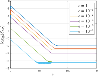
Figure 1: Time evolution of $\mathcal{E}_{\rm AP}$ with different $\epsilon$. The $x$-axis is time $t$, and the $y$-axis is $\log_{10}(\mathcal{E}_{\rm AP})$.

In this test, the mesh size is $N=100$ and the expansion order of the $P_{N}$ method is $M=7$. Since we are going to test the behavior of the numerical scheme when $\epsilon$ goes to zero, the time step is set as $\Delta t={\rm C}\Delta x^{2}/c$. Figure 1 shows the time evolution of $\mathcal{E}_{\rm AP}$ as

$$\mathcal{E}_{\rm AP}=\sqrt{\Delta x\sum_{i=1}^{N}\Big{(}(I_{0,i}-acT_{i}^{4})^{2}+\sum_{j=1}^{M}I_{j,i}^{2}\Big{)}},$$ (5.2)

for the numerical scheme (3.18) with different $\epsilon$. We can see that for any $\epsilon$, $\mathcal{E}_{\rm AP}$ is decreasing with time and then reaches a final steady state. With the decreasing of $\epsilon$, the final value of $\mathcal{E}_{\rm AP}$ becomes smaller, which shows the AP property of the numerical scheme.

Next, we test the order of the numerical scheme (3.18). The initial data (5.1) with the same parameters are applied. We compute the solutions with grid size $N=50,100,200,400$ and $800$, respectively for $\epsilon=1,0.1$ and $0.01$. The final time is $t=0.5$, and the numerical solution with $N=1600$ is chosen as the reference solution. The $l_{2}$ error between the numerical solution and the reference solution with different $\epsilon$ is calculated. Figure 2 shows the convergence order of the numerical method for different $\epsilon$. It illustrates that for different $\epsilon$, the scheme is the uniformly first-order, which also validates the AP property of the numerical scheme.

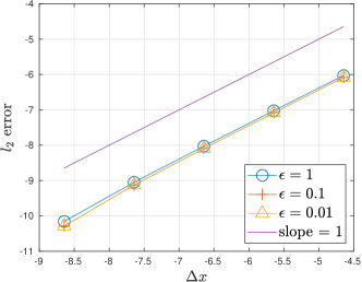
(a) $I$

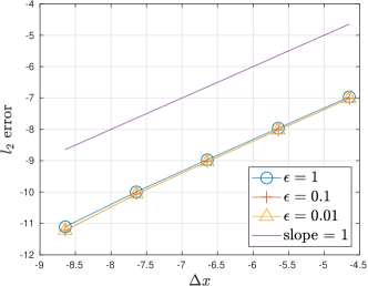
(b) $T$

Figure 2: $l_{2}$ error between the numerical solution with grid size $N=50,100,200,400$ and $800$ and the reference solution $N=1600$. (a) The $l_{2}$ error of the specific intensity $I$. (b) The $l_{2}$ error of the material temperature $T$.

To further verify the AP property of this numerical scheme, we redo the test with higher-order scheme. First, the linear reconstruction with IMEX3 scheme is utilized. The grid size is set as $N=100,200,400,800$, respectively for $\epsilon=1,0.1,0.01,10^{-6}$. The numerical solution with $N=1600$ is chosen as the reference solution. The final time is $t=0.5$, and the $l_{2}$ error between the numerical solution and the reference solution with different $\epsilon$ is calculated. Figure 3 shows the convergence order of the numerical method for different $\epsilon$. It illustrates that for different $\epsilon$, the scheme is the uniformly second-order.

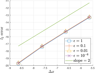
(a) $I$

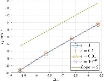
(b) $T$

Figure 3: $l_{2}$ error with linear reconstruction between the numerical solution with grid size $N=100,200,400$ and $800$ and the reference solution is $N=1600$. (a) The $l_{2}$ error of the specific intensity $I$. (b) The $l_{2}$ error of the material temperature $T$.

With the same settings as above, we will test the convergence order of the numerical method for different $\epsilon$ by IMEX3 scheme with the third-order WENO reconstruction. The numerical results are shown in Figure 4. We could see that the convergence order of different $\epsilon$ is the same. However, it is only second-order. We have studied the reason carefully, and a simple proof is proposed in Appendix A.5.

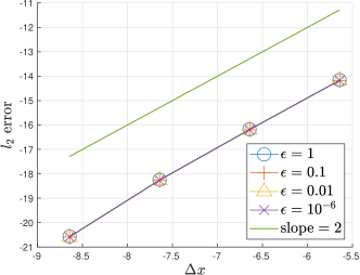
(a) $I$

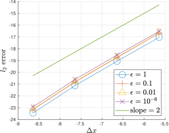
(b) $T$

Figure 4: $l_{2}$ error with third-order WENO reconstruction between the numerical solution with grid size $N=100,200,400$ and $800$ and the reference solution $N=1600$. (a) The $l_{2}$ error of the specific intensity $I$. (b) The $l_{2}$ error of the material temperature $T$.

To record the evolution of the temperature $T$ with $\epsilon$, the evolution of $T$ for different $\epsilon$ is plotted in Figure 5, where two positions $x=0.505$ and $1.005$ are recorded. Here, the grid size is $N=200$, and $\epsilon=1,0.5,10^{-2},10^{-6}$. The evolution of the temperature $T$ of the nonlinear diffusion equation (2.7) is also plotted. From it, we can see that the temperature $T$ is converging to the solution of the nonlinear diffusion equation as $\epsilon$ approaches zero. The behavior of $T$ also validates the stability of the numerical scheme when $\epsilon$ goes to zero.

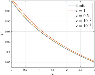
(a) $x=0.505$

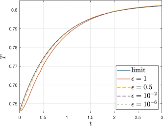
(b) $x=1.005$

Figure 5: The evolution of temperature $T$ with time increasing for different $\epsilon$. (a) The value of $T$ at $x=0.505$. (b) The value of $T$ at $x=1.005$.

5.2 Marshak wave problems

In the following examples, the classical Marshak wave problems are tested. The Marshak problem is one of the benchmark problems and is also studied in the literature such as [43, 24, 31]. In the computations, the parameters are chosen the same as that in [43] with $a=0.01372\rm{GJ/cm^{3}-keV^{4}}$ and $c=29.98\rm{cm/ns}$. In this section, two absorption/emission coefficients are tested. For both cases, the inflow boundary condition is imposed on both the left and right sides, where the Marshak type boundary condition [31] is utilized. The details of the Marshak type boundary are proposed in Appendix A.2.

Marshak Wave-2B

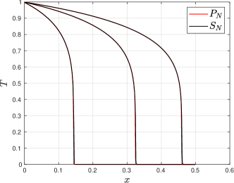
(a) material temperature

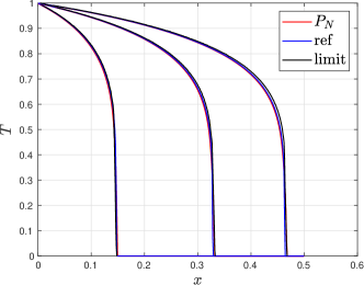
(b) material temperature

Figure 6: The material temperature $T$ of Marshak Wave-2B problem at time $t=10,50$ and $100$. The left picture is the $P_{N}$ solution and the reference solution get by $S_{N}$ method. The right picture is the $P_{N}$ solution and the reference solution in [31] and the black line is that to the diffusion limit.

In this example, we take the absorption/emission coefficient to be $\sigma=100/{\rm T^{3}cm^{2}/g}$, the density to be $3.0\rm{g/cm^{3}}$ and the specific heat to be $0.1\rm{GJ/g/keV}$. The initial material temperature $T$ is set to be $10^{-6}{\rm keV}$. A constant isotropic incident specific intensity with a Planckian distribution at $1$ keV is kept on the left boundary. The computation domian is $[0,\infty)$ but taken to be $L=[0,0.2]$ in the simulations. In this case, $\sigma$ is large enough that the solution to RTE is almost the same as that of the diffusion limit (2.7).

In the test, the expansion order of $P_{N}$ is set as $M=11$ with the grid size $N=400$. The third-order IMEX RK scheme (3.22) is applied here, where the time step is set as

$$\Delta t=C\Delta x/c.$$ (5.3)

In Figure 6, the numerical results of the radiation wave front at time $t=10,50$ and $100$ are plotted. In Figure 6a, the reference is obtained by the $S_{N}$ method, and in Figure 6b, the reference solution is from [31] and the diffusion limit result is produced by the finite difference method. From Figure 6, we can find that the numerical solution to RTE is on top of each other with that of the reference solution and the diffusion limit results, which is also consistent with the expectation that the solution to RTE is almost the same as the diffusion limit.

Marshak Wave-2A

Marshak Wave-2A problem is quite similar to Marshak Wave-2B problem, except that its absorption/emission coefficient is $\sigma=10{\rm/T^{3}cm^{2}/g}$. In this case, since $\sigma$ is not large enough, the solution to RTE is different from that of the diffusion limit.

In this test, the same numerical setting as Marshak wave-2B problem is chosen. In Figure 7a, the computed radiation wave front at time $t=0.2,0.4,0.6,0.8$ and $1.0$ are given and the reference is obtained from the $S_{N}$ method. Figure 7b presents the computed material temperature for both the gray approximation to the radiation transfer equations and the nonlinear diffusion equation at time $t=1$, where the reference solution is from [19]. From it, we can see that the numerical solution matches the reference solution well, but is quite different from the diffusion limit.

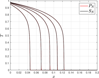
(a) material temperature

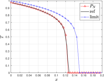
(b) material temperature

Figure 7: The material temperature $T$ of Marshak Wave-2A problem at different time. (a) The material temperature $T$ of Marshak Wave-2A problem at $t=0.2,0.4,0.6,0.8$ and $1$. The black line is the reference solution obtained by $S_{N}$ method. (b) The material temperature $T$ of Marshak Wave-2A problem at $t=1$, where the red line is the numerical solution to RTE, the black line is the reference solution and the blue line is that to diffusion limit.

From the numerical results of Marshak wave problems, we can find that the new numerical scheme works well both for the optically thick and thin problems. The time step length is independent of the absorption coefficients $\sigma$, which shows the high efficiency of this AP numerical scheme.

5.3 A lattice problem

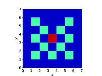
Figure 8: Layout of the lattice problem.

In this section, we study a two-dimensional problem with the added complication of multiple materials but without radiation-material coupling. We consider the transfer equation

$$\dfrac{\epsilon^{2}}{c}\dfrac{\partial{I}}{\partial{t}}+\epsilon\boldsymbol{\Omega}\cdot\nabla I=-\sigma_{a}I+\sigma_{s}\left(\dfrac{1}{4\pi}\int_{\mathbb{S}^{2}}I\,\mathrm{d}\boldsymbol{\Omega}-I\right)+\epsilon^{2}G.$$ (5.4)

Photons are absorbed with a power density of $\dfrac{c\sigma_{a}}{\epsilon^{2}}I$. As there is no radiation-material coupling, the photons are simply removed from the system when the absorption occurs. The isotropic scattering term does not change the radiation temperature but causes the specific intensity $I$ to become more evenly distributed in microscopic velocity. The computation domain is $[0,7]\times[0,7]$. It consists of a set of squares belonging to a strongly absorbing medium in a background of weakly scattering medium. The specific layout of the problem is given in Figure 8, where the blue regions and the dark red region are purely scattering medium with $\sigma_{s}=1$ and $\sigma_{a}=0$; the light green regions contain purely absorbing material with $\sigma_{s}=0$ and $\sigma_{a}=10$. In the dark red region, there is an isotropic source $G=\dfrac{1}{4\pi}$, and $G$ is zero elsewhere. Initially the specific intensity is at equilibrium and the radiation temperature is $10^{-6}$. Vacuum boundary conditions are imposed on all four sides of the computation domain, which means there is an outflow of radiation but no inflow. The detailed application of the inflow boundary is proposed in Appendix A.2, and we also refer to [31] for more details. Other parameters are set as $c=a=\epsilon=1$.

We use a mesh of $280\times 280$ in the spatial space and $P_{5}$ is adopted here. Moreover, the filtering technique is applied in the microscopic velocity space to avoid negative energy density solution. Filtering techniques as proposed in [32] are employed in 2D simulations to suppress spurious oscillations in $P_{N}$ solutions. The filtering applied here is only applied to $l\geqslant 2M/3$, where $M$ is the highest order of spherical harmonic expansion [10, 5]. For these $l$, before updating each time step, we substitute $I^{m}_{l}$ with $\hat{I}^{m}_{l}$. Precisely

$$\hat{I}^{m}_{l}=\dfrac{I^{m}_{l}}{1+\alpha l^{2}(l+1)^{2}},$$ (5.5)

where

$$\alpha=\dfrac{\omega}{M^{2}}\dfrac{1}{[(\sigma_{a}+\sigma_{s})L+M]^{2}},\qquad\omega=\dfrac{2c\Delta t}{\Delta x},$$ (5.6)

with $L$ the characteristic length of the problem, which is taken to be $L=1$ for all the simulations. $\sigma_{a}$ and $\sigma_{s}$ are the absorption and scattering coefficients, respectively.

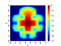
(a) $\log_{10}I^{0}_{0}$ by AP IMEX.

(b) $\log_{10}I^{0}_{0}$ by StaRMAP.

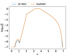
(c) $\log_{10}I^{0}_{0}$ at $x=3.5$

Figure 9: The contour and slice plot of $\log_{10}I^{0}_{0}$ for the lattice problem at $t=3.2$. (a) Contour plot of the AP numerical scheme. (b) The contour plot of the reference solution reproduced using StaRMAP. (c) Comparison between the numerical solution and the reference solution reproduced by StaRMAP at $x=3.5$.

In the test, the first-order scheme (3.18) is utilized for temporal discretization and a third-order WENO reconstruction is adopted in spatial discretization. The results at time $t=3.2$ are shown in Figure 9 with the logarithm of $I_{0}^{0}$ to the base 10 shown in contour and slice. The reference solution is obtained using StarRMAP [40, 41]. Figure 9 show that both solutions agree with each other quite well, and the beams of the particles leaking between the corners of the absorbing regions are all well produced. This phenomenon is also studied in [1, 41], and the behavior of the numerical results are almost the same.

5.4 A hohlraum problem

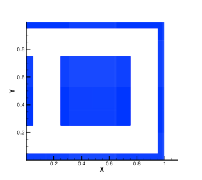
Figure 10: Layout of the hohlraum problem. The blue regions are where $(x,y)\in[0,0.05]\times[0.25,0.75]$, and $(x,y)\in[0.25,0.75]\times[0.25,0.75]$, $(x,y)\in[0,1]\times[0,0.05]$, $(x,y)\in[0,1]\times[0.95,1]$ and $(x,y)\in[0.95,1]\times[0,1]$.

This section studies the hohlraum problem, which is similar to that in [32]. For this problem, the radiation field is coupled with the material energy. It is well known that the diffusion approximation fails to capture the correct physics of this problem [1, 32], making it necessary to simulate the original RTE (2.1). Moreover, in this problem, the material is initially cold and optically thick, and then becomes optically thinner as radiation heats it up. The wide range in optical depth presents a challenge to the numerical schemes. The layout of the problem is shown in Figure 10. The computation domain is $[0,1]\times[0,1]$, where the white areas are vacuum with $\sigma_{a}=0$. The blue regions in Figure 10 satisfy $\sigma_{a}=100{\rm/T^{3}cm^{2}/g}$, while the density is $1.0\rm{g/cm^{3}}$ and the heat capacity $C_{v}$ is $0.3\rm{GJ/g/keV}$. An isotropic inflow of $1$ keV black body source is incident on the entire left boundary. For the boundary conditions, the Marshak type inflow boundary condition is applied. For the left boundary there is an isotropic inflow, and for other boundaries, the outside is treated as vacuum. Therefore, there is an outflow of radiation but no inflow in other three boundaries. The details of the Marshak type inflow are also proposed in Appendix A.2. In the simulation, the related parameters are set as $\epsilon=1$, $a=0.01372\rm{GJ/cm^{3}-keV^{4}}$ and $c=29.98\rm{cm/ns}$. The mesh size is $100\times 100$ in the spatial space and the $P_{N}$ method with $M=7$ is utilized. The first-order scheme for the time discretization and third-order WENO reconstruction in the spatial discretization is utilized here with the same filtering techniques in the last section.

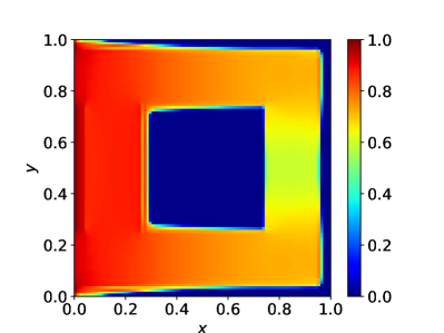
(a) Radiation temperature

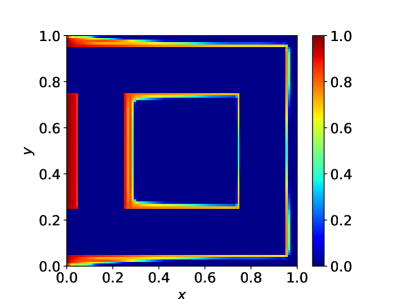
(b) Material temperature

Figure 11: The contour plots of radiation and material temperature of the hohlraum problem produced by the AP scheme at $t=1$. (a) Radiation temperature. (b) Material temperature.

Figure 11 presents the contour plots of the numerical solution for the radiation temperature and the material temperature at $t=1$, where the radiation temperature is defined as

$$T_{\rm rad}=\sqrt[4]{\dfrac{I^{0}_{0}}{ac}}.$$ (5.7)

As is stated in [32] that the solution to this problem has two properties, first of which is the non-uniform heating of the central block, and the other is less radiation directly behind the block than those regions within the line of source sight. The same phenomenon could also be found in the numerical results here. Moreover, the numerical results also show that the photons could bend around the front wall and the back wall is starting to heat up and re-emit photons. The numerical solutions along $y=0.125$ and $x=0.85$ are plotted in Figure 12, where the solution obtained by IMC method [32] is also plotted. We can find that the numerical solutions are in rough agreement with the IMC solution.

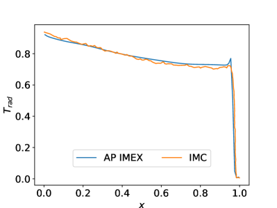
(a) $y=0.125$

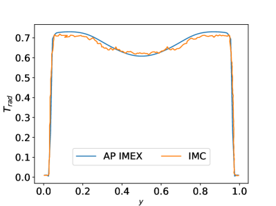
(b) $x=0.85$

Figure 12: The radiation temperature of the hohlraum problem at $t=1$ on different slices. Here, the blue line the numerical solution by the AP numerical method, and the red line is the reference solution by IMC method in [32]. (a) radiation temperature $T_{\rm rad}$ at $y=0.125$. (b) radiation temperature $T_{\rm rad}$ at $x=0.85$.

6 Conclusions

In this paper, we have developed an AP IMEX numerical scheme for the RTE system in the framework of $P_{N}$ method. The Chapman-Enskog expansion is utilized to derive the order of each expansion coefficient of the specific intensity respected to the mean free path. Thus, in each equation of the $P_{N}$ system, the terms at lower-order of the mean free path are set as an implicit term with those at higher-order set as an explicit term. Therefore, the implicit-explicit $P_{N}$ system can be solved at the computational cost of a completely explicit scheme with the time step length independent of the mean free path. The analysis of the total energy shows the energy stability with the evolution of time. Numerical examples have exhibited the AP property and the efficiency of this new scheme. However, this method is limited to the gray approximation of the radiative transfer equations for the moment. Research works on the frequency-dependent problem are ongoing.

Appendix A Appendix

A.1 The gray approximation of the radiative transfer equations for 1D angle problem and related $P_{N}$ equations

The time-dependent gray approximation of the radiative transfer equations [31] in a one-dimensional planar geometry medium have the form as

$$\frac{\epsilon^{2}}{c}\dfrac{\partial{I}}{\partial{t}}+\epsilon\mu\dfrac{\partial{I}}{\partial{x}}=\sigma\left(\frac{1}{2}acT^{4}-I\right),\qquad x\in[0,L],$$ (A.1a)

$$\epsilon^{2}C_{v}\dfrac{\partial{T}}{\partial{t}}=\sigma\left(\int_{-1}^{1}I\,\mathrm{d}\mu-acT^{4}\right),$$ (A.1b)

where $I(t,x,\mu)$ is the specific intensity of radiation, $\mu=\cos\theta\in[-1,1]$ is the internal coordinate associated with the angle $\theta\in[0,\pi]$. $T(t,x)$ is the material temperature, and $\sigma$ is the absorption opacity. Moreover, the one-dimensional form of (2.10) is reduced into

$$\frac{\epsilon^{2}}{c}\dfrac{\partial{I}}{\partial{t}}+\epsilon\mu\dfrac{\partial{I}}{\partial{x}}=\sigma\left(\frac{1}{2}\int I\,\mathrm{d}\mu-I\right),\qquad x\in[0,L].\\$$ (A.2)

For (A.1), the basis function for the $P_{N}$ method is the Legendre polynomials. The moments are defined as

$$I_{l}=\int_{-1}^{1}P_{l}(\mu)I(t,x,\mu)\,\mathrm{d}\mu,\qquad l=0,\cdots M,$$ (A.3)

where $P_{l}$ is the Legendre polynomial. Then, the $P_{N}$ equations for (A.1) are

$$\frac{\epsilon^{2}}{c}\dfrac{\partial{\bar{{\bf I}}}}{\partial{t}}+\epsilon{\bf B}^{\rm low}\dfrac{\partial{\bar{{\bf I}}}}{\partial{x}}+\epsilon{{\bf B}}^{\rm up}\dfrac{\partial{{\bar{{\bf I}}}}}{\partial{x}}=-\sigma{\bar{{\bf I}}}+\sigma acT^{4}e_{1},$$ (A.4)

$$\epsilon^{2}C_{v}\dfrac{\partial{T}}{\partial{t}}=\sigma\left(I_{0}-acT^{4}\right),$$

where $\bar{{\bf I}}=(I_{0},I_{1},\cdots,I_{M})$ and $e_{1}=(1,0,\cdots,0)^{T}$. ${\bf B}^{\rm low}$ and ${\bf B}^{\rm up}$ are triangular matrix with the non-zero entries as

$${\bf B}^{\rm low}(i+1,i)=\frac{i}{2i+1},\qquad{\bf B}^{\rm up}(i,i+1)=\frac{i}{2(i-1)+1},\qquad i=1,\cdots M.$$ (A.5)

A.2 Inflow boundary condition for $P_{N}$ equations

We implement the inflow boundary condition for the $P_{N}$ equations by specifying the values of coefficients of the $P_{N}$ system in ghost cells. Choosing the left boundary as an example, the incoming specific intensity incident on the boundary interface is

$$I(\mu)=I^{b}(\mu),\quad\text{for}~{}\mu>0.$$ (A.6)

For the $P_{N}$ method, the numerical boundary can be rewritten as

$$I^{\rm ghost}(\mu)=\left\{\begin{array}[]{cc}I^{b}(\mu),&\mu>0,\\ I^{i}(\mu),&\mu<0,\end{array}\right.$$ (A.7)

where $I^{i}(\mu)$ is the specific intensity at the left boundary of the area. Then, the expansion coefficient at the ghost cell is

$$I^{\rm ghost}_{l}=\int_{-1}^{1}I^{\rm ghost}(\mu)P_{l}(\mu)\,\mathrm{d}\mu.$$ (A.8)

The implementation of the inflow boundary condition in 2D is similar in spirit to that of 1D. Supposing $\boldsymbol{n}$ is the outward normal of the boundary interface, the incident specific intensity on the boundary is

$$I(\boldsymbol{\Omega})=I^{b}(\boldsymbol{\Omega}),\quad\text{for}~{}\boldsymbol{\Omega}\cdot\boldsymbol{n}<0.$$ (A.9)

For the $P_{N}$ method, the numerical boundary can be rewritten as

$$I^{\rm ghost}(\boldsymbol{\Omega})=\left\{\begin{array}[]{cc}I^{b}(\boldsymbol{\Omega}),&\boldsymbol{\Omega}\cdot\boldsymbol{n}<0,\\ I^{i}(\boldsymbol{\Omega}),&\boldsymbol{\Omega}\cdot\boldsymbol{n}>0,\end{array}\right.$$ (A.10)

where $I^{i}(\boldsymbol{\Omega})$ is the specific intensity on the interior side of the boundary interface. Thus, the expansion coefficient at the ghost cell is

$$I^{m,\rm ghost}_{l} =\int_{\mathbb{S}^{2}}I^{\rm ghost}(\boldsymbol{\Omega})\overline{Y^{m}_{l}}(\boldsymbol{\Omega})\,\mathrm{d}\boldsymbol{\Omega}$$ (A.11)

$$=\int_{\boldsymbol{\Omega}\cdot\boldsymbol{n}<0}I^{b}(\boldsymbol{\Omega})\overline{Y^{m}_{l}}(\boldsymbol{\Omega})\,\mathrm{d}\boldsymbol{\Omega}+\int_{\boldsymbol{\Omega}\cdot\boldsymbol{n}>0}I^{i}(\boldsymbol{\Omega})\overline{Y^{m}_{l}}(\boldsymbol{\Omega})\,\mathrm{d}\boldsymbol{\Omega}$$

$$=\int_{\boldsymbol{\Omega}\cdot\boldsymbol{n}<0}I^{b}(\boldsymbol{\Omega})\overline{Y^{m}_{l}}(\boldsymbol{\Omega})\,\mathrm{d}\boldsymbol{\Omega}+\sum\limits_{j=0}^{M}\sum\limits_{k=-j}^{j}I^{k,i}_{j}\int_{\boldsymbol{\Omega}\cdot\boldsymbol{n}>0}Y^{k}_{j}(\boldsymbol{\Omega})\overline{Y^{m}_{l}}(\boldsymbol{\Omega})\,\mathrm{d}\boldsymbol{\Omega}.$$

The integration $\int_{\boldsymbol{\Omega}\cdot\boldsymbol{n}>0}Y^{k}_{j}(\boldsymbol{\Omega})\overline{Y^{m}_{l}}(\boldsymbol{\Omega})\,\mathrm{d}\boldsymbol{\Omega}$ does not depend on the specific numerical solutions, and is pre-computed.

A.3 Proof of Proposition 2

In this section, the proof of the Proposition 2 is proposed here.

Proof of Proposition 2.

Following the method in [39], we will begin the Fourier analysis of (3.18) for the $P_{1}$ system of the linear equation system (A.2). The result can be extended to the generalized $P_{N}$ system naturally. We will first discuss two special cases where $\xi=0,\pi$. Therein, $\bf C$ is reduced into a real diagonal matrix with the maximum eigenvalues equaling $1$. According to the principle, the numerical scheme is stable.

Then, we study the general case by considering two scenarios according to the time step length:

1. $\epsilon<\Delta x$, where

   $$\Delta t=C\Delta x^{2}.$$ (A.12)

   Substituting the time step length (A.12) into (3.36), we can find that $\lambda_{i},i=1,2$ are functions of $C$, $\frac{\epsilon}{\Delta x}$, $\alpha$ and $\xi$. Introducing two variables as $\beta_{1}=\log_{10}(C)$ and $\beta_{2}=\log_{10}(\epsilon/\Delta x)$, the stability regions are plotted in Figure 13 with fixed $\alpha$. Here the discrete wave number $\xi$ is uniformly taken from $[0,2\pi]$ with $200$ samples. In this case, due to the definition of $C$ which is the CFL number and $\epsilon<\Delta x$, the range for $\beta_{1}$ and $\beta_{2}$ is changed into

   $$\beta_{1}<0,\qquad\beta_{2}<0.$$ (A.13)

   Moreover, it is natural to demand that $\epsilon<\Delta x<0.4$. Thus, $\alpha$ is taken uniformly from $[0,\exp(-1/0.16)]$ with 100 samples and six cases are shown in Figure 13 due to their similar behavior. From Figure 13, we can find that when $\alpha=0$, the numerical scheme is always stable. However, with the increase of $\alpha$, the stability region is becoming smaller, especially when the CFL number $C$ is large and the radio $\epsilon/\Delta x$ is small. We find that when $\alpha=\exp(-1/0.16)$, the numerical scheme is stable when $\log_{10}(\epsilon/\Delta x)>-2.5$. Noting that when $\alpha=\exp(-1/0.16)$, which means $\epsilon=0.4$, $\log_{10}(\epsilon/\Delta x)$ is always larger than $-2.5$ for $\Delta x<1$. This indicates that in the simulation of benchmark problems, the stability condition is always satisfied.

2. $\epsilon>\Delta x$, where

   $$\Delta t=C\epsilon\Delta x.$$ (A.14)

   Substituting the time step length (A.14) into (3.36), we can easily find that $\lambda_{i},i=1,2$ are also the function of $C$, $\frac{\epsilon}{\Delta x}$, $\alpha$ and $\xi$. Introducing the same two variables $\beta_{i},i=1,2$, we plot the stability regions in Figure 14 with fixed $\alpha$. Here the discrete wave number $\xi$ is uniformly taken from $[0,2\pi]$ with $200$ samples. Since

   $$\alpha=\exp\left(-\frac{1}{\epsilon^{2}}\right),$$ (A.15)

   and assuming $\epsilon<1$ in the numerical test, $\alpha$ is taken uniformly from $[0,0.5]$ with 100 samples. As their behavior is similar, the six cases $\alpha=0,0.05,0.1,0.2,0.3$ and $0.5$ are plotted here to illustrate the result. Moreover, due to the definition of $C$ which is the CFL number, and the condition that $\epsilon>\Delta x$, it holds that

   $$\beta_{1}<0,\qquad\beta_{2}>0.$$ (A.16)

   From Figure 14, we can find that the numerical scheme is stable under the time step length (A.14). In the numerical tests, the upper bound of $\epsilon$ is $\epsilon=10^{5}\Delta x$, which is large enough for the computational parameter.

(a) $\alpha=0$

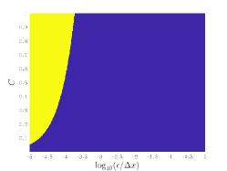
(b) $\alpha=0.1\exp(-1/0.16)$

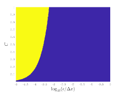
(c) $\alpha=0.3\exp(-1/0.16)$

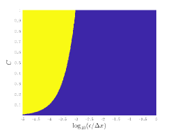
(d) $\alpha=0.5\exp(-1/0.16)$

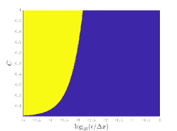
(e) $\alpha=0.8\exp(-1/0.16)$

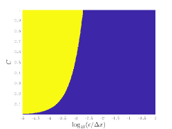
(f) $\alpha=\exp(-1/0.16)$

Figure 13: The stability region for the numerical scheme (3.18) of $P_{1}$ system under the condition (A.12). The $x$-axis is $\beta_{2}=\log_{10}(\epsilon/\Delta x)$, and the $y$-axis is the CFL number $C$. The blue region is the area where the numerical scheme is stable and the yellow region is the area where the numerical scheme is unstable.

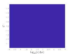
(a) $\alpha=0$

(b) $\alpha=0.05$

(c) $\alpha=0.1$

(d) $\alpha=0.2$

(e) $\alpha=0.3$

(f) $\alpha=0.5$

Figure 14: The stability region for the numerical scheme (3.18) of $P_{1}$ system under the condition (A.14). The $x$-axis is $\beta_{2}=\log_{10}(\epsilon/\Delta x)$, and the $y$-axis is the CFL number $C$. The blue region is the area where the numerical scheme is stable.

∎

A.4 Proof of Theorem 2

In this section, the proof of Theorem 2 is proposed here.

Proof of Theorem 2.

We will take $M=2$ as an example, and it could be extended to the general case naturally. Moreover, without loss of generality, we set $a=c=C_{v}=\sigma=1$ in the proof. When $M=2$, (4.10) is reduced into

$$\epsilon^{2}\frac{I_{0,j}^{n+1}-I_{0,j}^{n}}{\Delta t} +\epsilon\frac{I_{1,j+1}^{n}-I_{1,j-1}^{n}}{2\Delta x}-\frac{\alpha\epsilon}{2}\frac{I_{0,j+1}^{n}-2I_{0,j}^{n}+I_{0,j-1}^{n}}{\Delta x}=\left((T_{j}^{4})^{n+1}-I_{0,j}^{n+1}\right),$$ (A.17a)

$$\epsilon^{2}\frac{I_{1,j}^{n+1}-I_{1,j}^{n}}{\Delta t} +\frac{\epsilon}{3}\frac{I_{0,j+1}^{n+1}-I_{0,j-1}^{n+1}}{2\Delta x}+\frac{2\epsilon}{3}\frac{I_{2,j+1}^{n}-I_{2,j-1}^{n}}{2\Delta x}-\frac{\alpha\epsilon}{2}\frac{I_{1,j+1}^{n}-2I_{1,j}^{n}+I_{1,j-1}^{n}}{\Delta x}=-I_{1,j}^{n+1},$$ (A.17b)

$$\epsilon^{2}\frac{I_{2,j}^{n+1}-I_{2,j}^{n}}{\Delta t} +\frac{2\epsilon}{5}\frac{I_{1,j+1}^{n+1}-I_{1,j-1}^{n+1}}{2\Delta x}-\frac{\alpha\epsilon}{2}\frac{I_{2,j+1}^{n}-2I_{2,j}^{n}+I_{2,j-1}^{n}}{\Delta x}=-I_{2,j}^{n+1},$$ (A.17c)

$$\epsilon^{2}\frac{T_{j}^{n+1}-T_{j}^{n}}{\Delta t} +\epsilon\frac{I_{0,j}^{n+1}-I_{0,j}^{n}}{\Delta t}+\epsilon\frac{I_{1,j+1}^{n}-I_{1,j-1}^{n}}{2\Delta x}-\frac{\alpha\epsilon}{2}\frac{I_{0,j+1}^{n}-2I_{0,j}^{n}+I_{0,j-1}^{n}}{\Delta x}=0.$$ (A.17d)

For (A.17a), multiplying it by $I_{0,j}^{n+1}$, we can get that

$$\epsilon^{2}I_{0,j}^{n+1}\frac{I_{0,j}^{n+1}-I_{0,j}^{n}}{\Delta t}+\epsilon I_{0,j}^{n+1}\frac{I_{1,j+1}^{n}-I_{1,j-1}^{n}}{2\Delta x}-\frac{\alpha\epsilon}{2}I_{0,j}^{n+1}\frac{I_{0,j+1}^{n}-2I_{0,j}^{n}+I_{0,j-1}^{n}}{\Delta x}=I_{0,j}^{n+1}\left((T_{j}^{4})^{n+1}-I_{0,j}^{n+1}\right).$$ (A.18)

For (A.17b) and (A.17c), shifting it backward one time step and multiplying $3I_{1,j}^{n}$ and $5I_{2,j}^{n}$ respectively, we can derive that

$$3\epsilon^{2}I_{1,j}^{n}\frac{I_{1,j}^{n}-I_{1,j}^{n-1}}{\Delta t} +\epsilon I_{1,j}^{n}\frac{I_{0,j+1}^{n}-I_{0,j-1}^{n}}{2\Delta x}+\epsilon I_{1,j}^{n}\frac{I_{2,j+1}^{n-1}-I_{2,j-1}^{n-1}}{\Delta x}-\frac{3\alpha\epsilon}{2}I_{1,j}^{n}\frac{I_{1,j+1}^{n-1}-2I_{1,j}^{n-1}+I_{1,j-1}^{n-1}}{\Delta x}=-3(I_{1,j}^{n})^{2},$$ (A.19)

$$5\epsilon^{2}I_{2,j}^{n}\frac{I_{2,j}^{n}-I_{2,j}^{n-1}}{\Delta t} +\epsilon I_{2,j}^{n}\frac{I_{1,j+1}^{n}-I_{1,j-1}^{n}}{\Delta x}-\frac{5\alpha\epsilon}{2}I_{2,j}^{n}\frac{I_{2,j+1}^{n-1}-2I_{2,j}^{n-1}+I_{2,j-1}^{n-1}}{\Delta x}=-5(I_{2,j}^{n})^{2}.$$

Summing (A.18) and (A.19) over $j$, then it holds that

$$\frac{\epsilon^{2}}{2\Delta t}\sum_{j}\Big{[}(I_{0,j}^{n+1})^{2}-(I_{0,j}^{n})^{2}+3\left((I_{1,j}^{n})^{2}-(I_{1,j}^{n-1})^{2}\right)+5\left((I_{2,j}^{n})^{2}-(I_{2,j}^{n-1})^{2}\right)\Big{]}+A_{0}=A_{1}+A_{2}+A_{3},$$ (A.20)

where

$$A_{0} =\frac{\epsilon^{2}}{2\Delta t}\sum_{j}\Big{[}(I_{0,j}^{n+1}-I_{0,j}^{n})^{2}+3(I_{1,j}^{n}-I_{1,j}^{n-1})^{2}+5(I_{2,j}^{n}-I_{2,j}^{n-1})^{2}\Big{]},$$ (A.21a)

$$A_{1} =-\frac{\epsilon}{2\Delta x}\sum_{j}\Big{[}I_{0,j}^{n+1}(I_{1,j+1}^{n}-I_{1,j-1}^{n})+I_{1,j}^{n}(I_{0,j+1}^{n}-I_{0,j-1}^{n})+2I_{1,j}^{n}(I_{2,j+1}^{n-1}-I_{2,j-1}^{n-1})+2I_{2,j}^{n}(I_{1,j+1}^{n}-I_{1,j-1}^{n})\Big{]},$$ (A.21b)

$$A_{2} =\frac{\alpha\epsilon}{2\Delta x}\sum_{j}\Big{[}I_{0,j}^{n+1}(I_{0,j+1}^{n}-2I_{0,j}^{n}+I_{0,j-1}^{n})+3I_{1,j}^{n}(I_{1,j+1}^{n-1}-2I_{1,j}^{n-1}+I_{1,j-1}^{n-1})+5I_{2,j}^{n}(I_{2,j+1}^{n-1}-2I_{2,j}^{n-1}+I_{2,j-1}^{n-1})\Big{]},$$ (A.21c)

$$A_{3} =-\sum_{j}\Big{[}-I_{0,j}^{n+1}(T_{j}^{4})^{n+1}+(I_{0,j}^{n+1})^{2}+3(I_{1,j}^{n})^{2}+5(I_{2,j}^{n})^{2}\Big{]}.$$ (A.21d)

Then we will begin from the approximation of $A_{1}$ and $A_{2}$. With some arrangement and the periodic boundary condition, $A_{1}$ is changed into

$$A_{1}= -\frac{\epsilon}{2\Delta x}\sum_{j}\Big{[}(I_{0,j}^{n+1}-I_{0,j}^{n})(I_{1,j+1}^{n}-I_{1,j-1}^{n})+2(I_{1,j+1}^{n}-I_{1,j-1}^{n})(I_{2,j}^{n}-I_{2,j}^{n-1})\Big{]}$$ (A.22)

$$\leqslant \frac{\epsilon}{2\Delta x}\sum_{j}\Big{[}\frac{1}{2}\beta_{1}^{2}(I_{0,j}^{n+1}-I_{0,j}^{n})^{2}+\frac{1}{2\beta_{1}^{2}}(I_{1,j+1}^{n}-I_{1,j-1}^{n})^{2}+\beta_{2}^{2}(I_{2,j}^{n}-I_{2,j}^{n-1})^{2}+\frac{1}{\beta_{2}^{2}}(I_{1,j+1}^{n}-I_{1,j-1}^{n})^{2}\Big{]}$$

$$\leqslant \frac{\epsilon}{2\Delta x}\sum_{j}\Big{[}\frac{1}{2}\beta_{1}^{2}(I_{0,j}^{n+1}-I_{0,j}^{n})^{2}+\beta_{2}^{2}(I_{2,j}^{n}-I_{2,j}^{n-1})^{2}+\left(\frac{2}{\beta_{1}^{2}}+\frac{4}{\beta_{2}^{2}}\right)(I_{1,j}^{n})^{2}\Big{]}.$$

With the estimation that

$$\sum_{j}I_{0,j}^{n+1}(I_{0,j+1}^{n}-2I_{0,j}^{n}+I_{0,j-1}^{n})$$ (A.23)

$$\qquad=\sum_{j}\Big{[}(I_{0,j}^{n+1}-I_{0,j}^{n})(I_{0,j+1}^{n}-2I_{0,j}^{n}+I_{0,j-1}^{n})+I_{0,j}^{n}(I_{0,j+1}^{n}-2I_{0,j}^{n}+I_{0,j-1}^{n})\Big{]}$$

$$\qquad\leqslant\sum_{j}\Big{[}\frac{1}{2}\beta_{3}^{2}(I_{0,j}^{n+1}-I_{0,j}^{n})^{2}+\frac{2}{\beta_{3}^{2}}(I_{0,j}^{n}-I_{0,j-1}^{n})^{2}\Big{]}-\sum_{j}(I_{0,j}^{n}-I_{0,j-1}^{n})^{2}$$

$$\qquad=\sum_{j}\Big{[}\frac{1}{2}\beta_{3}^{2}(I_{0,j}^{n+1}-I_{0,j}^{n})^{2}+(\frac{2}{\beta_{3}^{2}}-1)\left(I_{0,j}^{n}-I_{0,j-1}^{n}\right)^{2}\Big{]}.$$

Similarly, it also holds that

$$\sum_{j}I_{1,j}^{n}(I_{1,j+1}^{n-1}-2I_{1,j}^{n-1}+I_{1,j-1}^{n-1}) =\sum_{j}I_{1,j}^{n-1}(I_{1,j+1}^{n}-2I_{1,j}^{n}+I_{1,j-1}^{n})$$ (A.24)

$$\leqslant\sum_{j}\Big{[}\frac{1}{2}\beta_{4}^{2}(I_{1,j}^{n}-I_{1,j}^{n-1})^{2}+4\left(\frac{2}{\beta_{4}^{2}}-1\right)(I_{1,j}^{n})^{2}\Big{]},$$

$$\sum_{j}I_{2,j}^{n}(I_{2,j+1}^{n-1}-2I_{2,j}^{n-1}+I_{2,j-1}^{n-1}) =\sum_{j}I_{2,j}^{n-1}(I_{2,j+1}^{n}-2I_{2,j}^{n}+I_{2,j-1}^{n})$$

$$\leqslant\sum_{j}\Big{[}\frac{1}{2}\beta_{5}^{2}(I_{2,j}^{n}-I_{2,j}^{n-1})^{2}+\left(\frac{2}{\beta_{5}^{2}}-1\right)(I_{2,j}^{n}-I_{2,j-1}^{n})^{2}\Big{]}.$$

Let

$$\beta_{1}^{2}=\frac{2\epsilon\Delta x}{\Delta t}-2\alpha,\qquad\beta_{2}^{2}=\frac{5\epsilon\Delta x}{\Delta t}-5\alpha,\qquad\beta_{3}^{2}=2,\qquad\beta_{4}^{2}=\frac{2\Delta x\epsilon}{\alpha\Delta t},\qquad\beta_{5}^{2}=2,$$ (A.25)

then together with (A.21), (A.22), (A.23), (A.24) and (A.25), (A.20) is reduced into

$$\begin{split}\frac{\epsilon^{2}}{2}\sum_{j}\Big{[}(I_{0,j}^{n+1})^{2}-(I_{0,j}^{n})^{2}+3\left((I_{1,j}^{n})^{2}-(I_{1,j}^{n-1})^{2}\right)+5\left((I_{2,j}^{n})^{2}-(I_{2,j}^{n-1})^{2}\right)\Big{]}\\ \leqslant\beta_{6}\sum_{j}(I_{1,j}^{n})^{2}+\Delta t\sum_{j}\Big{[}I_{0,j}^{n+1}(T_{j}^{4})^{n+1}-(I_{0,j}^{n+1})^{2}-5(I_{2,j}^{n})^{2}\Big{]},\end{split}$$ (A.26)

with

$$\beta_{6}=\frac{9}{10}\dfrac{\epsilon\Delta t}{\Delta x}\left(\frac{1}{\frac{\epsilon\Delta x}{\Delta t}-\alpha}\right)+\dfrac{6\alpha^{2}(\Delta t)^{2}}{(\Delta x)^{2}}-\dfrac{6\alpha\epsilon\Delta t}{\Delta x}-3\Delta t.$$ (A.27)

If it holds for $\beta_{6}$ that

$$\beta_{6}\leqslant 0,$$ (A.28)

with the time step length (3.32), then we can derive the stability result (4.16). Precisely, with (A.17a) and (A.17d), we can derive that

$$\epsilon^{2}\frac{T_{j}^{n+1}-T_{j}^{n}}{\Delta t}=-(T_{j}^{4})^{n+1}+I_{0,j}^{n+1}.$$ (A.29)

Multiplying (A.29) with $(T_{j}^{4})^{n+1}$ and summing over $j$, it holds with (A.26)

$$\begin{split}&\sum_{j}\left[\frac{\epsilon^{2}}{2\Delta t}\Big{(}(I_{0,j}^{n+1})^{2}-(I_{0,j}^{n})^{2}+3\left[(I_{1,j}^{n})^{2}-(I_{1,j}^{n-1})^{2}\right]+5\left[(I_{2,j}^{n})^{2}-(I_{2,j}^{n-1})^{2}\right]\Big{)}\right.\\ &\qquad\left.+\frac{\epsilon^{2}}{5\Delta t}\Big{[}(T_{j}^{5})^{n+1}-(T_{j}^{5})^{n}\Big{]}\right]\leqslant-\sum_{j}\left[I_{0,j}^{n+1}-(T_{j}^{4})^{n+1}\right]^{2}\leqslant 0.\end{split}$$ (A.30)

We derive the energy stability (4.16). The only point left is to prove (A.28), which we will be done in two cases:

1. $\epsilon>\Delta x$, in which case,

   $$\Delta t=C\epsilon\Delta x.$$ (A.31)

   Substituting (A.31) into (A.27), we can deduce that

   $$\beta_{6}=\frac{9C^{2}\epsilon^{2}}{10}\left(\frac{1}{1-\alpha C}\right)+6\alpha\epsilon^{2}C(\alpha C-1)-3C\Delta x\epsilon.$$ (A.32)

   Thus if

   $$0<C<\min\left(\frac{\epsilon}{\alpha\Delta x},\frac{10\Delta x}{3\epsilon+10\Delta x\alpha}\right),$$ (A.33)

   it holds that $\beta_{6}\leqslant 0$.

   For the coefficients $\beta_{i}^{2},i=1,\cdots 5$, it requires that $\beta_{i}^{2}>0$. Thus, from (A.25), it demands that

   $$\frac{\epsilon\Delta x}{\Delta t}-\alpha>0.$$ (A.34)

   Substituting (A.31) into (A.34), we can obtain that

   $$C<\frac{1}{\alpha}.$$ (A.35)

   Thus, the constrain on $C$ is changed into

   $$0<C<\min\left(\frac{1}{\alpha},\frac{10\Delta x}{3\epsilon+10\Delta x\alpha}\right).$$ (A.36)

2. $\epsilon<\Delta x$, in which case

   $$\Delta t=C\Delta x^{2}.$$ (A.37)

   Substituting (A.37) into (A.27), we can deduce that

   $$\beta_{6}=\frac{9}{10}C^{2}\epsilon\Delta x^{2}\left(\frac{1}{\epsilon-\alpha C\Delta x}\right)+6\alpha\Delta xC(\alpha C\Delta x-\epsilon)-3C\Delta x^{2}.$$ (A.38)

   Thus if

   $$0<C<\min\left(\frac{\epsilon}{\alpha\Delta x},\frac{10\epsilon}{3\epsilon+10\Delta x\alpha}\right),$$ (A.39)

   it holds that $\beta_{6}\leqslant 0$. Similarly, we can verify that the constrain $\beta_{i}^{2}>0,i=1,\cdots 5$ will not affect the condition (A.39), then the proof is finished.

   For $\epsilon<\Delta x$, it is always true that $\alpha=\exp(-1/\epsilon^{2})$ is quite small, and (A.39) could be reduced into

   $$0<C<\frac{10}{3}.$$ (A.40)

∎

A.5 Analysis of the higher-order scheme

From the test of the AP property for the numerical scheme, we found that even for the IMEX3 scheme with WENO reconstruction, the convergence order is only two. Analysis of the numerical scheme shows that when solving $T^{n+1}$, the fourth-order polynomial equation of $T^{n+1}$ is solved, where $(T^{n+1})^{4}$ is approximated as

$$(T^{4})_{i}\approx(T_{i})^{4}$$ (A.41)

instead of

$$(T)^{4}_{i}\approx\frac{\int_{x_{i-\frac{1}{2}}}^{x_{i+\frac{1}{2}}}T^{4}dx}{\Delta x},$$ (A.42)

where $T_{i}$ is the cell average of cell $i$. Noting that

$$\frac{\int_{x_{i-\frac{1}{2}}}^{x_{i+\frac{1}{2}}}T(x)dx}{\Delta x}=T(x_{i})+\frac{1}{24}(T(\xi_{i}))^{{}^{\prime\prime}}\Delta x^{2},\quad\xi\in[x_{i-\frac{1}{2}},x_{i+\frac{1}{2}}],$$ (A.43)

and

$$\frac{\int_{x_{i-\frac{1}{2}}}^{x_{i+\frac{1}{2}}}T^{4}(x)dx}{\Delta x}=T^{4}(x_{i})+\frac{1}{24}(T^{4}(\eta_{i}))^{{}^{\prime\prime}}\Delta x^{2},\eta_{i}\in[x_{i-\frac{1}{2}},x_{i+\frac{1}{2}}],$$ (A.44)

thus, it holds

$$\frac{\int_{x_{i-\frac{1}{2}}}^{x_{i+\frac{1}{2}}}T^{4}dx}{\Delta x}-(T_{i})^{4}=\mathcal{O}(\Delta x^{2}).$$ (A.45)

Therefore, the convergence order of the whole numerical scheme is at most two.

References

- [1] T. A. Brunner. Forms of approximate radiation transport. Sandia report, 2002.
- [2] A. Crestetto, N. Crouseilles, G. Dimarco, and M. Lemou. Asymptotically complexity diminishing schemes (ACDS) for kinetic equations in the diffusive scaling. J. Comput. Phys., 394:243–262, 2019.
- [3] J. Densmore. Asymptotic analysis of the spatial discretization of radiation absorption and re-emission in Implicit Monte Carlo. J. Comput. Phys., 230(4):1116–1133, 2011.
- [4] J. Densmore, H. Park, A. Wollaber, R. Rauenzahn, and D. Knoll. Monte Carlo simulation methods in moment-based scale-bridging algorithms for thermal radiative-transfer problems. J. Comput. Phys., 284:40–58, 2015.
- [5] Y. Di, Y. Fan, Z. Kou, R. Li, and Y. Wang. Filtered hyperbolic moment method for the Vlasov equation. J. Sci. Comput., 79(2):969–991, 2019.
- [6] N. Discacciati, J. Hesthaven, and R. Deep. Controlling oscillations in high-order Discontinuous Galerkin schemes using artificial viscosity tuned by neural networks. J. Comput. Phys., 409:109304, 2020.
- [7] J. Fleck and J. Cummings. An implicit Monte Carlo scheme for calculating time and frequency dependent nonlinear radiation transport. J. Comput. Phys., 8(3):313–342, 1971.
- [8] N. Gentile. Implicit Monte Carlo diffusion-an acceleration method for Monte Carlo time-dependent radiative transfer simulations. J. Comput. Phys., 172(2):543–571, 2001.
- [9] H. Hammer, H. Park, and L. Chacón. A multi-dimensional, moment-accelerated deterministic particle method for time-dependent, multi-frequency thermal radiative transfer problems. J. Comput. Phys., 386:653–674, 2019.
- [10] T. Hou and R. Li. Computing nearly singular solutions using pseudo-spectral methods. J. Comput. Phys., 226(1):379–397, 2007.
- [11] J. Jang, F. Li, J. Qiu, and T. Xiong. Analysis of asymptotic preserving dg-imex schemes for linear kinetic transport equations in a diffusive scaling. SIAM J. Numer. Anal., 52(4):2048–2072, 2014.
- [12] J. Jang, F. Li, J. Qiu, and T. Xiong. High order asymptotic preserving DG-IMEX schemes for discrete-velocity kinetic equations in a diffusive scaling. J. Comput. Phys., 281:199–224, 2015.
- [13] S. Jin and C. Levermore. The discrete-ordinate method in diffusive regimes. Transp. Theory Stat. Phys, 20(1-2):413–439, 1991.
- [14] S. Jin and C. Levermore. Fully discrete numerical transfer in diffusive regimes. Transp. Theory Stat. Phys, 22(6):739–791, 1993.
- [15] S. Jin, L. Pareschi, and G. Toscani. Uniformly accurate diffusive relaxation schemes for multiscale transport equations. SIAM J. Numer. Anal., 38(3):913–936, 2000.
- [16] D. Kershaw. Flux limiting nature’s own way. Technical Report UCRL-78378, Lawrence Livermore National Laboratory, Livermore, CA, 1976.
- [17] A. Klar. An asymptotic-induced scheme for nonstationary transport equations in the diffusive limit. SIAM J. Numer. Anal, 35(6):1073–1094, 1998.
- [18] R. Koch, W. Krebs, S. Wittig, and R. Viskanta. Discrete ordinates quadrature schemes for multidimensional radiative transfer. J. Quant. Spectrosc. Ra., 53(4):353–372, 1995.
- [19] Los Alamos National Laboratory. An implicit Monte Carlo code for thermal radiative transfer: Capabilities, development, and usag. LA-14195-MS, 2000.
- [20] V. Laboure, R. McClarren, and C. Hauck. Implicit filtered for high-energy density thermal radiation transport using discontinuous galerkin finite elements. J. Comput. Phys., 321:624–643, 2016.
- [21] M. Laiu, M. Frank, and C. Hauck. A positive asymptotic-preserving scheme for linear kinetic transport equations. SIAM J. Sci. Comput., 41:A1500–A1526, 2019.
- [22] A. Larsen and J. Morel. Asymptotic solutions of numerical transport problems in optically thick, diffusive regimes. J. Comput. Phys., 69(2):283–324, 1987.
- [23] A. Larsen and J. Morel. Asymptotic solutions of numerical transport problems in optically thick, diffusive regimes. ii. J. Comput. Phys., 83(1):212–236, 1989.
- [24] E. Larsen, A. Kumar, and J. Morel. Properties of the implicitly time-differenced equations of thermal radiation transport. J. Comput. Phys., 238:82–96, 2013.
- [25] K. Lathrop and B. Garlson. Discrete ordinates angular quadrature of the neutron transport equation. Los Alamos Scientific Laboratory, 1965.
- [26] E. Lemou and L. Mieussens. A new asymptotic preserving scheme based on micro-macro formulation for linear kinetic equations in the diffusion limit. SIAM J. Sci. Comput., 31:334–368, 2010.
- [27] E. Lewis and W. Miller. Computational Methods in Neutron Transport. United States, 1993.
- [28] W. Li, C. Liu, Y. Zhu, J. Zhang, and K. Xu. Unified gas-kinetic wave-particle methods iii: Multiscale photon transport. J. Comput. Phys., 408:109280, 2020.
- [29] P. Maginot, J. Ragusa, and J. Morel. High-order solution methods for grey discrete ordinates thermal radiative transfer. J. Comput. Phys., 327:719–746, 2016.
- [30] K. Mathews. On the propagation of rays in discrete ordinates. Nucl. Sci. Eng., 132:155–180, 1999.
- [31] R. McClarren, T. Evans, R. Lowrie, and J. Densmore. Semi-implicit time integration for PN thermal radiative transfer. J. Comput. Phys., 227(16):7561–7586, 2008.
- [32] R. McClarren and C. Hauck. Robust and accurate filtered spherical harmonics expansions for radiative transfer. J. Comput. Phys., 229(16):5597–5614, 2010.
- [33] R. McClarren and C. Hauck. Simulating radiative transfer with filtered spherical harmonics. Phys. Lett. A, 374(22):2290–2296, 2010.
- [34] R. McClarren, J. Holloway, and T. Brunner. On solutions to the equations for thermal radiative transfer. J. Comput. Phys., 227(5):2864–2885, 2008.
- [35] L. Mieussens. On the asymptotic preserving property of the unified gas kinetic scheme for the diffusion limit of linear kinetic models. J. Comput. Phys., 253:138–156, 2013.
- [36] J. Morel, T. Wareing, R. Lowrie, and D. Parsons. Analysis of ray-effect mitigation techniques. Nucl. Sci. Eng., 144:1–22, 2003.
- [37] G. Olson. Second-order time evolution of equations for radiation transport. J. Comput. Phys., 228(8):3072–3083, 2009.
- [38] H. Park, D. Knoll, R. Rauenzahn, A. Wollaber, and J. Densmore. A consistent, moment-based, multiscale solution approach for thermal radiative transfer problems. Transp. Theory Stat. Phys., 41(3-4):284–303, 2012.
- [39] Z. Peng, Y. Cheng, J. Qiu, and F. Li. Stability-enhanced AP IMEX-LDG schemes for linear kinetic transport equations under a diffusive scaling. J. Comput. Phys., 415:109485, 2020.
- [40] B. Seibold and M. Frank. Starmap code. website.http://www.math.temple.edu/ seibold/research/starmap.
- [41] B. Seibold and M. Frank. Starmap-a second order staggered grid method for spherical harmonics moment equations of radiative transfer. ACM T. Math. Software (TOMS), 41(1):4, 2014.
- [42] Y. Shi, P. Song, and W. Sun. An asymptotic preserving unified gas kinetic particle method for radiative transfer equations. J. Comput. Phys., 420:109687, 2020.
- [43] W. Sun, S. Jiang, and K. Xu. An asymptotic preserving unified gas kinetic scheme for gray radiative transfer equations. J. Comput. Phys., 285(15):265–279, 2015.
- [44] W. Sun, S. Jiang, and K. Xu. An asymptotic preserving implicit unified gas kinetic scheme for frequency-dependent radiative transfer equations. Int. J. Numer. Anal. Mod., 15(1-2):134–153, 2018.
- [45] M. Tang, L. Wang, and X. Zhang. Accurate front capturing asymptotic preserving scheme for nonlinear gray radiative transfer equation. SIAM J. Sci. Comput., 43(3):B759–B783, 2021.
- [46] J. Warsa, T. Wareing, and J. Morel. Krylov iterative methods and the degraded effectiveness of diffusion synthetic acceleration for multidimensional calculations in problems with material discontinuities. Nucl. Sci. Eng., 147:218–248, 2004.
- [47] T. Xiong, J. Jang, F. Li, and J. Qiu. High order asymptotic preserving nodal discontinuous Galerkin IMEX schemes for the BGK equation. J. Comput. Phys., 284:70–94, 2015.
- [48] T. Xiong, W. Sun, Y. Shi, and P. Song. High order asymptotic preserving discontinuous Galerkin methods for gray radiative transfer equations. arXiv:2011.14090, 2020.
- [49] B. Yan and S. Jin. A successive penalty-based asymptotic-preserving scheme for kinetic equations. SIAM J. Sci. Comput., 35(1):A150–A172, 2013.