On Efficient Low Distortion Ultrametric Embedding

Abstract

A classic problem in unsupervised learning and data analysis is to find simpler and easy-to-visualize representations of the data that preserve its essential properties. A widely-used method to preserve the underlying hierarchical structure of the data while reducing its complexity is to find an embedding of the data into a tree or an ultrametric. The most popular algorithms for this task are the classic linkage algorithms (single, average, or complete). However, these methods on a data set of $n$ points in $\Omega(\log n)$ dimensions exhibit a quite prohibitive running time of $\Theta(n^{2})$.

In this paper, we provide a new algorithm which takes as input a set of points $P$ in $\mathbb{R}^{d}$, and for every $c\geq 1$, runs in time $n^{1+\frac{\rho}{c^{2}}}$ (for some universal constant $\rho>1$) to output an ultrametric $\Delta$ such that for any two points $u,v$ in $P$, we have $\Delta(u,v)$ is within a multiplicative factor of $5c$ to the distance between $u$ and $v$ in the “best” ultrametric representation of $P$. Here, the best ultrametric is the ultrametric $\widetilde{\Delta}$ that minimizes the maximum distance distortion with respect to the $\ell_{2}$ distance, namely that minimizes $\underset{u,v\in P}{\max}\ \nicefrac{{\widetilde{\Delta}(u,v)}}{{\|u-v\|_{2}}}$.

We complement the above result by showing that under popular complexity theoretic assumptions, for every constant $\varepsilon>0$, no algorithm with running time $n^{2-\varepsilon}$ can distinguish between inputs in $\ell_{\infty}$-metric that admit isometric embedding and those that incur a distortion of $\nicefrac{{3}}{{2}}$.

Finally, we present empirical evaluation on classic machine learning datasets and show that the output of our algorithm is comparable to the output of the linkage algorithms while achieving a much faster running time.

1 Introduction

The curse of dimensionality has ruthlessly been haunting machine learning and data mining researchers. On the one hand, high dimensional representation of data elements allows fine-grained description of each datum and can lead to more accurate models, prediction and understanding. On the other hand, obtaining a significant signal in each dimension often requires a huge amount of data and high-dimensional data requires algorithms that can efficiently handle it. Hence, computing a simple representation of a high-dimensional dataset while preserving its most important properties has been a central problem in a large number of communities since the 1950s.

Of course, computing a simple representation of an arbitrary high-dimensional set of data elements necessarily incurs some information loss. Thus, the main question has been to find dimensionality reduction techniques that would preserve – or better, reveal – some structure of the data. An example of such a successful approach has been the principal component analysis which can be used to denoise a dataset and obtain a low-dimensional representation where ‘similar’ data elements are mapped to close-by locations. This approach has thus become a widely-used, powerful tool to identify cluster structures in high-dimensional datasets.

Yet, in many cases more complex structures underlie the datasets and it is crucial to identify this structure. For example, given similarity relations between species, computing a phylogenetic tree requires more than identifying a ‘flat’ clustering structure, it is critical to identify the whole hierarchy of species. Thus, computing a simple representation of an input containing a hierarchical structure has drawn a lot of attention over the years, in particular from the computational biology community. The most popular approaches are arguably the linkage algorithms, average-linkage, single-linkage, Ward’s method, and complete-linkage, which produce an embedding of the original metric into an ultrametric, see for example the seminal work of [CM10]. Unfortunately, these approaches come with a major drawback: all these methods, have quadratic running time – even in the best case – when the input consists of points in $\Theta(\log n)$ dimensions (where $n$ is the number of points) making them impractical for most applications nowadays. Obtaining an efficient algorithm for computing “good” hierarchical representation has thus been a major problem (see Section 1.2 for more details).

In this paper we are interested in constructing embeddings that (approximately) preserve the hierarchical structure underlying the input. For example, given three points $a,b,c$, we would like that if $a$ is more similar to $b$ than to $c$ (and so $a$ is originally closer to $b$ than to $c$ in the high-dimensional representation), then the distance of $a$ to $b$ in the ultrametric is lower than its distance to $c$. More formally, given a set of points $X$ in Euclidean space, a good ultrametric representation $\Delta$ is such that for every two points $a,b$ in $X$, we have

$$\|a-b\|_{2}\leq\Delta(a,b)\leq\alpha\cdot\|a-b\|_{2},$$

for the smallest possible $\alpha$ (see formal definition in Section 2). Interestingly, and perhaps surprisingly, this problem can be solved in $O(n^{2}d+n^{2}\log n)$ using an algorithm by [FKW95]. Unfortunately, this algorithm also suffers from a quite prohibitive quadratic running time. We thus ask:

Is there an easy-to-implement, efficient algorithm for finding
good ultrametric representation of high-dimensional inputs?

1.1 Our Results

We focus on the problem mentioned above, which we refer to as the Best Ultrametric Fit problem ($\mathsf{ULT}$) and which is formally defined in Section 2. We provide a simple algorithm, with running time $O(nd)+n^{1+O(1/\gamma^{2})}$ that returns a $5\gamma$-approximation for the $\mathsf{ULT}$ problem, or a near-linear time algorithm that returns an $O(\sqrt{\log n})$-approximation.

Theorem 1.1 (Upper Bound).

For any $\gamma>1$, there is an algorithm that produces a $5\gamma$-approximation in time $nd+n^{1+O(1/\gamma^{2})}$ for Euclidean instances of $\mathsf{ULT}$ of dimension $d$.
Moreover, there is an algorithm that produces an $O(\sqrt{\log n})$-approximation in time $O(nd+n\log^{2}n)$ for Euclidean instances of $\mathsf{ULT}$ of dimension $d$.

From a theoretical point of view, note that we can indeed get rid of the $nd$ dependency in the above theorem and replace it with an optimal bound depending on the number of non-zero coordinates by applying a sparse Johnson-Lindenstrauss transform in the beginning. Nonetheless, we stuck to the $nd$ dependency as it keeps the presentation of our algorithm simple and clear, and also since this is what we use in the experimental section.

Importantly, and perhaps surprisingly, we show that finding a faster than $n^{2-\varepsilon}$ algorithm for this problem is beyond current techniques.

Theorem 1.2 (Lower Bound; Informal version of Theorem 5.1).

Assuming $\mathsf{SETH}$, for every $\varepsilon>0$, no algorithm running in time $n^{2-\varepsilon}$ can determine if an instance of $\mathsf{ULT}$ of points in $\ell_{\infty}$-metric admits an isometric embedding or every embedding has distortion at least $3/2$.

We also provide inapproximability results for the Euclidean metric by ruling out $(1+o(1))$-approximation algorithms for $\mathsf{ULT}$ running in time $n^{1+o(1)}$ albeit under a more non-standard hypothesis that we motivate and introduce in this paper (see Theorem 5.7 for details).

Empirical results

We implemented our algorithm and performed experiments on three classic datasets (DIABETES, MICE, PENDIGITS). We compared the results with classic linkage algorithms (average, complete, single) and Ward’s method from the Scikit-learn library [PVG⁺11]. For a parameter $\gamma$ fixed to $\approx 2.5$, our results are as follows. First, as complexity analysis predicts, the execution of our algorithm is much faster whenever the dataset becomes large enough: up to $\approx 36$ (resp. $32$, $7$ and $35$) times faster than average linkage (resp. complete linkage, single linkage and Ward’s method) for moderate size dataset containing roughly $10000$ points, and has comparable running time for smaller inputs. Second, while achieving a much faster running time, the quality of the ultrametric stays competitive to the distortion produced by the other linkage algorithms. Indeed, the maximum distortion is, on these three datasets, always better than Ward’s method, while staying not so far from the others: in the worst case up to a factor $\approx 5.2$ (resp. $4.3$, $10.5$) against average linkage (resp. complete and single linkages). This shows that our new algorithm is a reliable and efficient alternative to the linkage algorithms when dealing with massive datasets.

1.2 Related Work

Strengthening the foundations for hierarchical representation of complex data has received a lot of attention over the years. The thorough study of [CM10] has deepened our understanding of the linkage algorithms and the inputs for which they produce good representations, we refer the reader to this work for a more complete introduction to the linkage algorithms. Hierarchical representation of data and hierarchical clusterings are similar problems. A recent seminal paper by [Das15] phrasing the problem of computing a good hierarchical clustering as an optimization problem has sparked a significant amount of work mixing theoretical and practical results. [CAKMTM18, MW17] showed that average-linkage achieves a constant factor approximation to (the dual of) Dasgupta’s function and introduced new algorithms with worst-case and beyond-worst-case guarantees, see also [RP16, CC17, CAKMT17, CCN19, CCNY18]. Single-linkage is also known to be helfpul to identify ‘flat’ clusterings in some specific settings [BBV08]. We would like to point out that this previous work did not consider the question of producing an ultrametric that is representative of the underlying (dis)similarities of the data and in fact most of the algorithms designed by previous work do not output ultrametrics at all. This paper takes a different perspective on the problem of computing a hierarchical clustering: we are interested in how well the underlying metric is preserved by the hierarchical clustering. Also it is worth mentioning that in [ABF⁺99, AC11] the authors study various tree embedding with a focus on average distortion in [AC11], and tree metrics (and not ultrametrics) in [ABF⁺99].

Finally, a related but orthogonal approach to ours was taken in recent papers by [CM15] and [ACH19]. There, the authors design implementation of average-linkage and Ward’s method that have subquadratic running time by approximating the greedy steps done by the algorithms. However, their results do not provide any approximation guarantees in terms of any objective function but rather on the quality of the approximation of the greedy step and is not guaranteed to produce an ultrametric.

1.3 Organization of Paper

This paper is organized as follows. In Section 2 we introduce the Farach et al. algorithm. In Section 3 we introduce our near linear time approximation algorithm for general metrics, and in Section 4 discuss its realization specifically in the Euclidean metric. In Section 5 we prove our conditional lower bounds on fast approximation algorithms. Finally, in Section 6 we detail the empirical performance of our proposed approximation algorithm.

2 Preliminaries

Formally, an ultrametric $(X,\Delta)$ is a metric space where for each $x,y,z\in X$,

$$\Delta(x,y)\leq\max(\Delta(x,z),\Delta(z,y)).$$

For all finite point-sets $X$, it can be (always) realized in the following way as well. Let $T=(V,E)$ be a finite, rooted tree, and let $L$ denote the leaves of $T$. Suppose $w:V\setminus L\to\mathbb{R}^{+}$ is a function that assigns positive weights to the internal vertices of $T$ such that the vertex weights are non-increasing along root-leaf paths. Then one can define a distance on $L$ by

$$d_{w}(\ell,\ell^{\prime}):=w(\mathsf{LCA}(\ell,\ell^{\prime})),$$

where $\mathsf{LCA}$ is the least common ancestor. This is an ultrametric on $L$.

We consider the Best Ultrametric Fit problem ($\mathsf{ULT}$), namely:

• Input: a set $V$ of $n$ elements $v_{1},\ldots,v_{n}$ and a weight function $w:V\times V\mapsto\mathbb{R}$.

• Output: an ultrametric $(V,\Delta)$ such that $\forall v_{i},v_{j}\in V$, $w(v_{i},v_{j})\leq\Delta(v_{i},v_{j})\leq\alpha\cdot w(v_{i},v_{j})$, for the minimal value $\alpha$.

Note that we will abuse notation slightly and, for an edge $e=(v_{i},v_{j})$, write $w(e)$ to denote $w(v_{i},v_{j})$. We write $\Delta^{{}_{\mathsf{OPT}}}$ to denote an optimal ultrametric, and let $\alpha_{{}_{\mathsf{OPT}}}$ denote the minimum $\alpha$ for which $\forall v_{i},v_{j}\in V$, $w(v_{i},v_{j})\leq\Delta^{{}_{\mathsf{OPT}}}(v_{i},v_{j})\leq\alpha\cdot w(v_{i},v_{j})$.

We say that an ultrametric $\widehat{\Delta}$ is a $\gamma$-approximation to $\mathsf{ULT}$ if $\forall v_{i},v_{j}\in V$, $w(v_{i},v_{j})\leq\widehat{\Delta}(v_{i},v_{j})\leq\gamma\cdot\alpha_{{}_{\mathsf{OPT}}}\cdot w(v_{i},v_{j})$.

2.1 Farach-Kannan-Warnow’s Algorithm

Farach et al. [FKW95] provide an $O(n^{2})$ algorithm to solve a “more general” problem (i.e., that is such that an optimal algorithm for this problem can be used to solve $\mathsf{ULT}$), the so-called “sandwich problem”. In the sandwich problem, the input consists of set $V$ of $n$ elements $v_{1},\ldots,v_{n}$ and two weight functions $w_{\ell}$ and $w_{h}$, and the goal is to output an ultrametric $(V,\Delta)$ such that $\forall v_{i},v_{j}\in V$, $w_{\ell}(v_{i},v_{j})\leq\Delta(v_{i},v_{j})\leq\alpha\cdot w_{h}(v_{i},v_{j})$ for the minimal $\alpha$. Observe that an algorithm that solves the sandwich problem can be used to solve Best Ultrametric Fit by setting $w_{\ell}=w_{h}=w$.

We now review the algorithm of [FKW95]. Given a tree $T$ over the elements of $V$ and an edge $e\in T$, removing $e$ from $T$ creates two connected components, we call $L(e)$ and $R(e)$ the set of elements in these connected components respectively. Given $L(e)$ and $R(e)$, we define $P(e)$ to be the set of pairs of elements $v_{i}\in L(e)$ and $v_{j}\in R(e)$ such that the maximum weight of an edge of the path from $v_{i}$ to $v_{j}$ in $T$ is $w_{\ell}(e)$.

A cartesian tree of a weighted tree $T$ is a rooted tree $T_{C}$ defined as follows: the root of $T_{C}$ corresponds to the edge of maximal weight and the two children of $T_{C}$ are defined recursively as the cartesian trees of $L(e)$ and $R(e)$, respectively. The leaves of $T_{C}$ correspond to the nodes of $T$. Each node has an associated height. The height of any leaf is set to $0$. For a non-leaf node $u\in T_{C}$, we know that $u$ corresponds, by construction, to an edge $e_{u}$ in $T$, which is the first edge (taken in decreasing order w.r.t. their weights) that separates $v_{i}$ from $v_{j}$ in $T$. Set the height of $u$ to be equal to the weight of $e_{u}$ in $T$. A cartesian tree $T_{C}$ naturally induces an ultrametric $\Delta$ on its leaves: the distance between two points $v_{i}$ and $v_{j}$ (i.e., two leaves of $T_{C}$) is defined as the height of their least common ancestor in $T_{C}$.

Finally, we define the cut weight of edge $e$ to be

$$CW(e)=\max_{(v_{i},v_{j})\in P(e)}w_{\ell}(v_{i},v_{j}).$$

The algorithm of [FKW95] is as follow:

1. Compute a minimum spanning tree (MST) $T$ over the complete graph $G_{h}$ defined on $V$ and with edge weights $w_{h}$;

2. Compute the cut weights with respect to the tree $T$;

3. Construct the cartesian tree $T_{C}$ of the tree $T^{\prime}$ whose structure is identical to $T$ and the distance from an internal node of $T_{C}$ to the leaves of its subtree is given by the cut weight of the corresponding edge in $T$.

4. Output the ultrametric induced by the tree metric of $T_{C}$.

The following theorem is proved in [FKW95]:

Theorem 2.1.

Given two weight functions $w_{\ell}$ and $w_{h}$, the above algorithm outputs an ultrametric $\Delta$ such that for all $v_{i},v_{j}\in V$

$$w_{\ell}(v_{i},v_{j})\leq\Delta(v_{i},v_{j})\leq\alpha_{{}_{\mathsf{OPT}}}\cdot w_{h}(v_{i},v_{j})$$

for the minimal $\alpha_{{}_{\mathsf{OPT}}}$.

3 ApproxULT: An Approximation Algorithm for $\mathsf{ULT}$

In this section, we describe a new approximation algorithm for $\mathsf{ULT}$ and prove its correctness. We then show in the next section how it can be implemented efficiently for inputs in the Euclidean metric.

Given a spanning tree $T$ over a graph $G$, any edge $e=(v_{i},v_{j})\in G\setminus T$ induces a unique cycle $C^{T}_{e}$ which consists of the union of $e$ and the unique path from $x$ to $y$ in $T$. We say that a tree $T$ is a $\gamma$-approximate Kruskal tree (or shortly a $\gamma$-KT) if

$$\forall e\in G\setminus T,w(e)\geq\frac{1}{\gamma}\max_{e^{\prime}\in C^{T}_{e}}{w(e^{\prime})}.$$

Moreover, given a tree $T$ and and an edge $e$ of $T$, we say that $\beta\in\mathbb{R}$ is a $\gamma$-estimate of $CW(e)$ if $CW(e)\leq\beta\leq\gamma\cdot CW(e)$. By extension, we say that a function

$$ACW:V\times V\mapsto\mathbb{R}$$

is a $\gamma$-estimate of the cut weights $CW$ if, for any edge $e$, $ACW(e)$ is a $\gamma$-estimate of $CW(e)$.

The rest of this section is dedicated to proving that the following algorithm achieves a $\gamma\delta$-approximation to $\mathsf{ULT}$, for some parameters $\gamma\geq 1,\delta\geq 1$ of the algorithm.

1. Compute a $\gamma$-KT $T$ over the complete graph $G_{h}$ defined on $V$ and with edge weights $w_{h}$;

2. Compute a $\delta$-estimate $ACW$ of the cut weights of all the edge of the tree $T$;

3. Construct the cartesian tree $T_{C}$ of the tree $T^{\prime}$ whose structure is identical to $T$ and the distance from an internal node of $T_{C}$ to the leaves of its subtree is given by the $ACW$ of the corresponding edge in $T$.

4. Output the ultrametric $\Delta$ over the leaves of $T_{C}$.

We want to prove the following:

Theorem 3.1.

For any $\gamma\geq 1,\delta\geq 1$, the above algorithm outputs an ultrametric $\Delta$ which is a $\gamma\delta$-approximation to $\mathsf{ULT}$, meaning that for all $v_{i},v_{j}\in V$

$$w_{\ell}(v_{i},v_{j})\leq\Delta(v_{i},v_{j})\leq\gamma\cdot\delta\cdot\alpha_{{}_{\mathsf{OPT}}}\cdot w_{h}(v_{i},v_{j})$$

Proof.

First step: we prove that the $\gamma$-KT $T$ computed at the first step of the algorithm can be seen an exact MST for a complete weighted graph $G^{\prime}$ defined on $V$ and with a weight function $w^{\prime}$ satisfying

$$\forall v_{i},v_{j}\in V,w^{\prime}(v_{i},v_{j})\leq\gamma\cdot w_{h}(v_{i},v_{j}).$$

We construct $w^{\prime}$ in the following way. For each pair of points $(v_{i},v_{j})$:

• If $(v_{i},v_{j})\in T$, then set $w^{\prime}(v_{i},v_{j})=w_{h}(v_{i},v_{j})$

• If $(v_{i},v_{j})\not\in T$, then set $w^{\prime}(v_{i},v_{j})=\gamma w_{h}(v_{i},v_{j})$.

By construction, it is clear that $w^{\prime}\leq\gamma\cdot w_{h}$. To see that $T$ is an (exact) MST of $G^{\prime}$, consider any MST $F$ of $G^{\prime}$. If $e=(v_{i},v_{j})\in F\setminus T$, then consider the first edge $e^{\prime}$ in the unique path from $v_{i}$ to $v_{j}$ in $T$ that reconnects $F\setminus e$. By definition of $w^{\prime}$, we have $w^{\prime}(e^{\prime})=w_{h}(e^{\prime})$ and $w^{\prime}(e)=\gamma w_{h}(e)$. Since $T$ is a $\gamma$-KT, we also have that $w_{h}(e)\geq\frac{1}{\gamma}w_{h}(e^{\prime})$. Therefore $w^{\prime}(e^{\prime})\leq w^{\prime}(e)$ and $\{F\cup e^{\prime}\}\setminus e$ is a spanning tree of $G^{\prime}$ of weight smaller than or equal to the weight of $F$. This proves that $\{F\cup e^{\prime}\}\setminus e$ is also a MST. Doing this process for all edges not in $T$ gives eventually $T$ and proves that $T$ is also a MST of $G^{\prime}$, as desired.

Second step. Observe that the weight function $w_{h}$ is not involved in steps 2, 3, and 4 of the algorithm. Therefore, if steps 2, 3, and 4 of the algorithm were made without approximation (meaning that we compute the exact cut weights $CW$ associated to the $\gamma$-KT tree $T$ and we output the ultrametric to the corresponding cartesian tree), then the output would be an ultrametric $\Delta$ such that for all $v_{i},v_{j}\in V$

$$w_{\ell}(v_{i},v_{j})\leq\Delta(v_{i},v_{j})\leq\alpha^{\prime}_{{}_{\mathsf{OPT}}}\cdot w^{\prime}(v_{i},v_{j})$$ (1)

for the minimal such $\alpha^{\prime}_{{}_{\mathsf{OPT}}}.$ This follows directly from Theorem 2.1 and the fact that $T$ is an exact MST for the graph $G^{\prime}$ defined above. Note that $\alpha^{\prime}_{{}_{\mathsf{OPT}}}\leq\alpha_{{}_{\mathsf{OPT}}}$ where $\alpha_{{}_{\mathsf{OPT}}}$ denotes the minimal constant such that there exists an ultrametric between $w_{l}$ and $\alpha_{{}_{\mathsf{OPT}}}\cdot w_{h}$.

Now, consider the ultrametric $\Delta^{T_{C}}$ associated to $T$ and a $\delta$-estimate $ACW$ of the cut weights. We claim that for all $v_{i},v_{j}\in V$

$$\Delta(v_{i},v_{j})\leq\Delta^{T_{C}}(v_{i},v_{j})\leq\delta\cdot\Delta(v_{i},v_{j}).$$ (2)

To see this, take any $v_{i},v_{j}\in V$. By definition, $\Delta^{T_{C}}(v_{i},v_{j})=ACW(e)$ for the first edge $e$ (taken in decreasing order w.r.t. to $ACW$) that separates $v_{i}$ from $v_{j}$ in $T$. Let $e_{v_{i},v_{j}}$ be the first edge that separates $v_{i}$ from $v_{j}$ w.r.t. to the actual cut weights $CW$. Again, we have by definition that $\Delta(v_{i},v_{j})=CW(e)$. We have that $ACW(e)\geq ACW(e_{v_{i},v_{j}})$ since $e$ is the first edge w.r.t. $ACW$. Moreover $ACW(e_{v_{i},v_{j}})\geq CW(e_{v_{i},v_{j}})$ because $ACW$ is a $\delta$-estimate of the cut weights: this gives us the first desired inequality

$$\Delta^{T_{C}}(v_{i},v_{j})\geq\Delta(v_{i},v_{j}).$$

The upper bound is similar. We know that $ACW(e)\leq\delta\cdot CW(e)$ since $ACW$ is a $\delta$-estimate. We also have that $CW(e)\leq CW(e_{v_{i},v_{j}})$ since $e_{v_{i},v_{j}}$ is the first separating edge w.r.t. $CW$. This gives:

$$\Delta^{T_{C}}(v_{i},v_{j})\leq\delta\cdot\Delta(v_{i},v_{j}).$$

All together, Equations 1 and 2 imply

$$w_{\ell}(v_{i},v_{j})\leq\Delta^{T_{C}}(v_{i},v_{j}) \leq\gamma\cdot\alpha^{\prime}_{{}_{\mathsf{OPT}}}\cdot w^{\prime}(v_{i},v_{j})$$

$$\leq\gamma\cdot\delta\cdot\alpha^{\prime}_{{}_{\mathsf{OPT}}}\cdot w_{h}(v_{i},v_{j})$$

$$\leq\gamma\cdot\delta\cdot\alpha_{{}_{\mathsf{OPT}}}\cdot w_{h}(v_{i},v_{j})$$

as desired. ∎

4 A Fast Implementation of ApproxULT in Euclidean Space – Proof of Theorem 1.1

In this section, we consider inputs of $\mathsf{ULT}$ that consists of a set of points $V$ in $\mathbb{R}^{d}$, and so for which $w(v_{1},v_{2})=\|v_{1}-v_{2}\|_{2}$. We now explain how to implement ApproxULT efficiently for $\gamma\geq 1$ and $\delta=5$.

Fast Euclidean $\gamma$-KT.

For computing efficiently a $\gamma$-KT of a set of points in a Euclidean space of dimension $d$, we appeal to the result of [HPIS13] (if interested in doubling metrics, one can instead use the bound of [FN18]). The approach relies on spanners; A $c$-spanner of a set $S$ of $n$ points in $\mathbb{R}^{d}$ is a graph $G=(S,E)$ and a weight function $w:E\mapsto\mathbb{R}_{+}$ such that for any $u,v\in S$, the shortest path distance in $G$ under the edge weights induced by $w$, $\Delta^{G}(u,v)$ satisfies $\|u-v\|_{2}\leq\Delta^{G}(u,v)\leq c\cdot\|u-v\|_{2}$.

The result of [HPIS13] states that there is an algorithm that for any set $S$ of $n$ points in $\mathbb{R}^{d}$ produces an $O(\gamma)$-spanner for $S$ with $O(n^{1+1/c^{2}}\log^{2}n)$ edges in time $O(nd+n^{1+1/c^{2}}\log^{2}n)$. The algorithm uses the locality sensitive hash family of [AI06], or alternatively for $\gamma=\sqrt{\log n}$ the Lipschitz partitions of [CCG⁺98].

An immediate application of Kruskal classic algorithm for computing a minimum spanning tree on the spanner yields an algorithm with running time $O(nd+n^{1+1/c^{2}}\log^{3}n)$. Moreover, we claim that a minimum spanning tree on a $c$-spanner $G$ is indeed a $c$-KT for the original point set. Assume towards contradiction that this is not the case. Then there exists an edge $e=(u,v)\not\in T$ such that $\|u-v\|_{2}<\max_{(x,y)\in C_{e}^{T}}\|x-y\|_{2}/c$. By correctness of the $c$-spanner we have that $\Delta^{G}(u,v)\leq c\|u-v\|_{2}<\max_{(x,y)\in C_{e}^{T}}\|x-y\|_{2}\leq\max_{(x,y)\in C_{e}^{T}}\Delta^{G}(x,y)$. A contradiction to the fact that $T$ is an MST of the $c$-spanner.

Fast Estimation of the Cut Weights.

We explain how to compute in time $O(nd+n\log n)$ a $5$-estimate of the cut weights. To do this, we maintain a disjoint-set data structure on $X$ with the additional property that each equivalence class $C$ (we call such an equivalence class cluster) has a special vertex $r_{C}$ and we store $m_{C}$ the maximal distance between $r_{C}$ and a point in the cluster. We now consider the edges of the MST $T$ in increasing order (w.r.t. their weights). When at edge $e=(x,y)$, we look at the two clusters $C$ and $D$ coming from the equivalence classes that respectively contain $x$ and $y$. We claim that

$$E=5\cdot\max(d(r_{C},r_{D}),m_{C}-d(r_{C},r_{D}),m_{D}-d(r_{C},r_{D}))$$

is a $5$-approximation of the cut weight for $e$. To see this, observe that if $x^{\prime},y^{\prime}$ are the farthest points respectively in $C,D$, then:

$$d(x^{\prime},y^{\prime}) \leq d(x^{\prime},r_{C})+d(r_{C},r_{D})+d(r_{D},y^{\prime})$$

$$\leq d(x^{\prime},r_{C})-d(r_{C},r_{D})+3d(r_{C},r_{D})+d(r_{D},y^{\prime})-d(r_{C},r_{D})$$

$$\leq 5.\max(d(r_{C},r_{D}),m_{C}-d(r_{C},r_{D}),m_{D}-d(r_{C},r_{D}))\leq E$$

On the other hand

$$d(r_{C},r_{D}) \leq d(x^{\prime},y^{\prime})$$

$$m_{C}-d(r_{C},r_{D}) \leq d(x^{\prime},r_{D})\leq d(x^{\prime},y^{\prime})$$

$$m_{D}-d(r_{C},r_{D}) \leq d(y^{\prime},r_{C})\leq d(x^{\prime},y^{\prime})$$

and therefore $E\leq 5\cdot d(x^{\prime},y^{\prime})$. Finally, if we consider the path from $x^{\prime}$ to $y^{\prime}$ in $T$, it is clear that the pair $(x^{\prime},y^{\prime})$ is in $P(e)$, and the bound on $CW(e)$ follows.

Merging $C$ and $D$ can simply be done via a classic disjoint-set data structure. Thus, the challenge is to update $m_{C\cup D}$. To do so, we consider the smallest cluster, say $D$, query $d(x,r_{C})$ for each point $x\in D$ and update accordingly $r_{C\cup D}$ if a bigger value is found. Therefore the running time to update $m_{C\cup D}$ is $O(|D|\times d)$ (we compute $|D|$ distances in a space of dimension $d$). The overall running time to compute the approximate cut weights is $O(nd+n\log n)$: sorting the edges requires $O(n\log n)$ and constructing bottom-up the cut-weights with the disjoint-set data structure takes $O(nd+n\alpha(n))$, where $\alpha(n)$ denotes the inverse of the Ackermann function (this part comes from the disjoint-set structure). To conclude, note that $n\alpha(n)$ is much smaller than $n\log n$.

5 Hardness of $\mathsf{ULT}$ for High-Dimensional Inputs

We complement Theorem 1.1 with a hardness of approximation result in this section. Our lower bound is based on the well-studied Strong Exponential Time Hypothesis ($\mathsf{SETH}$) [IP01, IPZ01, CIP06] which roughly states that SAT on $n$ variables cannot be solved in time less than $2^{n(1-o(1))}$. $\mathsf{SETH}$ is a popular assumption to prove lower bounds for problems in ¶ (see the following surveys [Wil15, Wil16, Wil18, RW19] for a discussion).

Theorem 5.1.

Assuming $\mathsf{SETH}$, for every $\varepsilon>0$, no algorithm running in time $n^{2-\varepsilon}$ can, given as input an instance of $\mathsf{ULT}$ consisting $n$ points of dimension $d:=O_{\varepsilon}(\log n)$ in $\ell_{\infty}$-metric, distinguish between the following two cases.

Completeness:

There is an isometric ultrametric embedding.

Soundness:

The distortion of the best ultrametric embedding is at least $\nicefrac{{3}}{{2}}$.

Note that the above theorem morally rules out approximation algorithms running in subquadratic time which can approximate the best ultrametric to $\nicefrac{{3}}{{2}}-o(1)$ factor.

Finally, we remark that all the results in this section can be based on a weaker assumption called the Orthogonal Vectors Hypothesis [Wil05] instead of $\mathsf{SETH}$. Before we proceed to the proof of the above theorem, we prove below a key technical lemma.

Definition 5.2 (Point-set $S^{*}$).

For every $\gamma,\gamma^{\prime}\geq 0$ and every $p\in\mathbb{R}_{\geq 1}\cup\{\infty\}$, we define the discrete point-set $S^{*}(\gamma,\gamma^{\prime},p):=\{a,a^{\prime},b\}$ in the $\ell_{p}$-metric as follows:

$$\|a-b\|_{p}\leq 1,\ \|a-a^{\prime}\|_{p}\leq 1+\gamma^{\prime},\text{ and }\|a^{\prime}-b\|_{p}\geq 1+\gamma.$$

Lemma 5.3 (Distortion in Ultrametric Embedding).

Fix $\gamma,\gamma^{\prime}\geq 0$ and $p\in\mathbb{R}_{\geq 1}\cup\{\infty\}$. Then we have that any embedding of $S^{*}(\gamma,\gamma^{\prime},p):=\{a,a^{\prime},b\}$ into ultrametric incurs a distortion of at least $\frac{1+\gamma}{1+\gamma^{\prime}}$.

Proof.

Let the distortion of $S^{*}$ to the ultrametric be at most $\rho$. Let $\tau$ be the embedding into ultrametric with distortion $\rho$ and let $\Delta$ denote distance in the ultrametric. Let $\alpha\in\mathbb{R}^{+}$ be the scaling factor of the embedding from the $\ell_{p}$-metric to the ultrametric.

$$(1+\gamma)\cdot\alpha \leq\Delta(\tau({a^{\prime}}),\tau({b}))$$

$$\leq\max\{\Delta(\tau(a),\tau(b)),\Delta(\tau(a),\tau({a^{\prime}}))\}$$

$$\leq\rho\cdot(1+\gamma^{\prime})\cdot\alpha$$

Thus we have that $\rho\geq\frac{1+\gamma}{1+\gamma^{\prime}}$. ∎

We combine the above lemma with David et al.’s conditional lower bound (stated below) on approximating the Bichromatic Closest Pair problem in the $\ell_{\infty}$-metric to obtain Theorem 5.1.

Theorem 5.4 ([DKL19]).

Assuming $\mathsf{SETH}$, for any $\varepsilon>0$, no algorithm running in time $n^{2-\varepsilon}$, given $A,B\subseteq\mathbb{R}^{d}$ as input, where $|A|=|B|=n$ and $d=O_{\varepsilon}(\log n)$, distinguish between the following two cases:

Completeness:

There exists $(a,b)\in A\times B$ such that $\|a-b\|_{\infty}=1$.

Soundness:

For every $(a,b)\in A\times B$ we have $\|a-b\|_{\infty}=3$.

Moreover this hardness holds even with the following additional properties:

• Every distinct pair of points in $A$ (resp. $B$) are at distance 2 from each other in the $\ell_{\infty}$-metric.

• All pairs of points in $A\times B$ are at distance either 1 or 3 from each other in the $\ell_{\infty}$-metric.

Proof of Theorem 5.1.

Let $(A,B)$ be the input to the hard instances of the Bichromatic Closest Pair problem as given in the statement of Theorem 5.4 (where $A,B\subseteq\mathbb{R}^{d}$ and $|A|=|B|=n$). We show that if for every $(a,b)\in A\times B$ we have $\|a-b\|_{\infty}=3$ then there is an isometric embedding of $A\cup B$ into an ultrametric and if there exists $(a,b)\in A\times B$ such that $\|a-b\|_{\infty}=1$ then any embedding of $A\cup B$ to an ultrametric incurs a distortion of $\nicefrac{{3}}{{2}}$. Once we show this, the proof of the theorem statement immediately follows.

Suppose that for every $(a,b)\in A\times B$ we have $\|a-b\|_{\infty}=3$. We construct the following ultrametric embedding. Let $T$ be a tree with root $r$. Let $r$ have two children $c_{A}$ and $c_{B}$. Both $c_{A}$ and $c_{B}$ each have $n$ leaves which we identify with the points in $A$ and points in $B$ respectively. Then we subdivide the edge between $c_{A}$ and its leaves and $c_{B}$ and its leaves. Notice that any pair of leaves corresponding to two distinct points in $A$ (resp. in $B$) are at distance four away in $T$. Also notice that any pair of leaves corresponding to a pair of points in $A\times B$ are at distance six. Therefore the aforementioned embedding is isometric.

Next, suppose that there exists $(a,b)\in A\times B$ such that $\|a-b\|_{\infty}=1$. We also suppose that there exists $(a^{\prime},b)\in A\times B$ such that $\|a^{\prime}-b\|_{\infty}=3$. We call Lemma 5.3 with the point-set $\{a,a^{\prime},b\}$ and parameters $\gamma=2$ and $\gamma^{\prime}=1$. Thus we have that even just embedding $\{a,a^{\prime},b\}$ into an ultrametric incurs distortion of $\nicefrac{{3}}{{2}}$. ∎

One may wonder if one can extend Theorem 5.1 to the Euclidean metric to rule out approximation algorithms running in subquadratic time which can approximate the best ultrametric to arbitrary factors close to 1. More concretely, one may look at the hardness of approximation results of [Rub18, KM19] on Closest Pair problem, and try to use them as the starting point of the reduction. An immediate obstacle to do so is that in the soundness case of the closest pair problem (i.e., the completeness case of the computing ultrametric distortion problem), there is no good bound on the range of all pairwise distances, and thus the distortion cannot be estimated to yield a meaningful reduction.

Nonetheless, we introduce a new complexity theoretic hypothesis below and show how that extends Theorem 5.1 to the Euclidean metric.

Colinearity Hypothesis.

Let $\mathcal{B}_{d}$ denote the $d$-dimensional unit Euclidean ball. In the Colinearity Problem ($\mathsf{CP}$), we are given as input a set $A$ of $n$ vectors uniformly and independently sampled from $\mathcal{B}_{d}$, and we move one of these sampled points to be closer to the midpoint of two other sampled points. The goal is to find these three points. More formally, we can write it as a decision problem in the following way.

Let $\mathcal{D}_{\texttt{uni}}$$(n,d)$ be the distribution which samples $n$ points uniformly and independently from $\mathcal{B}_{d}$. For every $\rho\in[0,1]$, let $\mathcal{D}_{\texttt{plant}}$$(n,d,\rho)$ be the following distribution:

1. Sample $(a_{1},\ldots,a_{n})\sim$$\mathcal{D}_{\texttt{uni}}$$(n,d)$.

2. Pick three distinct indices $i,j,k$ in $[n]$ at random.

3. Let $a_{i,j}$ be the midpoint of $a_{i}$ and $a_{j}$.

4. Let $\widetilde{a}_{k}$ be $(1-\rho)\cdot a_{k}+\rho\cdot a_{i,j}$.

5. Output $(a_{1},\ldots,a_{k-1},\widetilde{a}_{k},a_{k+1},\ldots,a_{n})$.

Notice that $\mathcal{D}_{\texttt{uni}}$$(n,d)$ $=$$\mathcal{D}_{\texttt{plant}}$$(n,d,0)$. Also, notice that in $\mathcal{D}_{\texttt{plant}}$$(n,d,1)$ we have planted a set of three colinear points. The decision problem $\mathsf{CP}$ would then be phrased as follows.

Definition 5.5 ($\mathsf{CP}$).

Let $\rho\in(0,1]$. Given as input a set of $n$ points sampled from $\mathcal{D}_{\texttt{uni}}$$(n,d)$ $\cup$ $\mathcal{D}_{\texttt{plant}}$$(n,d,\rho)$, distinguish if it was sampled from $\mathcal{D}_{\texttt{uni}}$$(n,d)$ or from $\mathcal{D}_{\texttt{plant}}$$(n,d,\rho)$.

The worst case variant of $\mathsf{CP}$ has been studied extensively in computational geometry and more recently in fine-grained complexity. In the worst case variant, we are given a set of $n$ points in $\mathbb{R}^{d}$ and we would like to determine if there are three points in the set that are colinear. This problem can be solved in time $O(n^{2}d)$. It’s now known that this runtime cannot be significantly improved assuming the 3-SUM hypothesis [GO95, GO12]. We putforth the following hypothesis on $\mathsf{CP}$:

Definition 5.6 (Colinearity Hypothesis ($\mathsf{CH}$)).

There exists constants $\rho,\varepsilon>0$ such that no randomized algorithm running in time $n^{1+\varepsilon}$ can decide $\mathsf{CP}$ (with parameters $n,d,\rho$), for every $d\geq O_{\rho,\varepsilon}(\log n)$.

Notice that unlike $\mathsf{OVH}$ or 3-SUM hypothesis, we are not assuming a subquadratic hardness for $\mathsf{CP}$, but only assume a superlinear hardness, as $\mathsf{CP}$ is closely related to the Light bulb problem [Val88], for which we do have subquadratic algorithms [Val15, KKK16, Alm19]. Elaborating, we now provide an informal sketch of a reduction from $\mathsf{CP}$ to the Light bulb problem: given $n$ points sampled from $\mathcal{D}_{\texttt{uni}}$$(n,d)$ $\cup$ $\mathcal{D}_{\texttt{plant}}$$(n,d,\rho)$, we first apply the sign function (+1 if the value is positive and -1 otherwise) to each coordinate of the sampled points, to obtain points on the Boolean hypercube. Then we only retain each point w.p. $\nicefrac{{1}}{{2}}$ and discard the rest. If the points were initially sampled from $\mathcal{D}_{\texttt{uni}}$$(n,d)$ then the finally retained points will look like points sampled uniformly and independently from the Boolean hypercube, whereas, if the points were initially sampled from $\mathcal{D}_{\texttt{plant}}$$(n,d,\rho)$ then there are two pairs of points that are $\rho^{\prime}$-correlated ($\rho^{\prime}$ depends on $\rho$) after applying the sign function and exactly one of the two pairs is retained with constant probability.

Returning to the application of $\mathsf{CH}$ to ultrametric embedding, assuming $\mathsf{CH}$, we prove the following result.

Theorem 5.7.

Assuming $\mathsf{CH}$, there exists $\varepsilon,\delta>0$ such that no randomized algorithm running in time $n^{1+\varepsilon}$ can given as input an instance of $\mathsf{ULT}$ consisting of $n$ points of dimension $d:=O_{\varepsilon,\delta}(\log n)$ in Euclidean metric distinguish between the following two cases.

Completeness:

The distortion of the best ultrametric embedding is at most $1+\nicefrac{{\delta}}{{2}}$.

Soundness:

The distortion of the best ultrametric embedding is at least $1+\delta$.

We use the following fact about random sampling from high-dimensional unit ball.

Fact 1 ([Ver18]).

For every $\delta>0$ there exists $c\in\mathbb{N}$ such that the following holds. Let $(a_{1},\ldots,a_{n})\sim$$\mathcal{D}_{\texttt{uni}}$$(n,c\cdot\log n)$. Then with high probability we have that for all distinct $i,j$ in $[n]$,

$$\|a_{i}-a_{j}\|_{2}\in(\beta-\delta,\beta+\delta),$$

for some universal scaling constant $\beta>1$.

Proof of Theorem 5.7.

Let $\varepsilon,\rho$ be the constants from $\mathsf{CH}$. Let $\delta:=\rho/9$ and $c$ be an integer guaranteed from Fact 1. Let $A$ be the input to $\mathsf{CP}$ (where $A\subseteq$$\mathcal{B}_{d}$ and $|A|=n$). We may assume that $d>c\log n$. We show that if all points in $A$ were picked independently and uniformly at random from $\mathcal{B}_{d}$ then there is an embedding of $A$ into an ultrametric with distortion less than $1+2\delta$ and if otherwise $A$ was sampled from $\mathcal{D}_{\texttt{plant}}$$(n,d,\gamma)$ then any embedding of $A$ to an ultrametric incurs a distortion of $1+4\delta$. Once we show this, the proof of the theorem statement immediately follows.

Suppose that $A$ was sampled from $\mathcal{D}_{\texttt{uni}}$$(n,d)$. From Fact 1 we have that for all distinct $a_{i},a_{j}$ in $A$,

$$\|a_{i}-a_{j}\|_{2}\in(\beta-\delta,\beta+\delta),$$

for some universal scaling constant $\beta>1$. Then the ultrametric embedding is simply given by identifying $A$ with the leaves of a star graph on $n+1$ nodes. The distortion in the embedding in such a case would be at most $\frac{\beta+\delta}{\beta-\delta}\leq 1+\nicefrac{{2\delta}}{{\beta}}<1+2\delta$.

Next, suppose that $A$ was sampled from $\mathcal{D}_{\texttt{plant}}$$(n,d,\rho)$. Then there exists 3 points $a_{i},a_{j},\widetilde{a}_{k}$ in $A$ such that the following distances hold:

$$\|a_{i}-a_{j}\|_{2} \geq\beta-\delta,$$

$$\|a_{i}-\widetilde{a}_{k}\|_{2},\|a_{j}-\widetilde{a}_{k}\|_{2} \leq\sqrt{(\nicefrac{{(\beta+\delta)}}{{2}})^{2}+\nicefrac{{3}}{{4}}((1-\rho)\cdot(\beta+\delta))^{2}}\leq\beta-\rho.$$

We call Lemma 4.3 with the point-set $\{a_{i},a_{j},\widetilde{a}_{k}\}$. Thus we have that even just embedding $\{a_{i},a_{j},\widetilde{a}_{k}\}$ into an ultrametric incurs distortion of $1+4\delta$. ∎

Note that we can replace $\mathsf{CH}$ by a search variant and this would imply the lower bound to the search variant of the $\mathsf{ULT}$ problem (unlike Theorem 4.1).

6 Experiments

We present some experiments performed on three standard datasets: DIABETES (768 samples, 8 features), MICE (1080 samples, 77 features), PENDIGITS (10992 samples, 16 features) and compare our C++ implementation of the algorithm described above to the classic linkage algorithms (average, complete, single or ward) as implemented in the Scikit-learn library (note that the Scikit-learn implementation is also in C++). The measure we are interested in is the maximum distortion $\max\limits_{(u,v)\in P}\frac{\Delta(u,v)}{\|u-v\|_{2}}$, where $P$ is the dataset and $\Delta$ the ultrametric output by the algorithm. Note that average linkage, single and ward linkage can underestimate distances, i.e., $\frac{\Delta(u,v)}{\|u-v\|_{2}}<1$ for some points $u$ and $v$. In practice, the smallest ratio given by average linkage lies often between $0.4$ and $0.5$ and between $0.8$ and $0.9$ for ward linkage. For single linkage, the maximum distortion is always $1$ and hence the minimum distortion can be very small. For a fair comparison, we normalize the ultrametrics by multiplying every distances by the smallest value for which $\frac{\Delta(u,v)}{\|u-v\|_{2}}$ becomes greater than or equal to $1$ for all pairs. Note that what matters most in hierarchical clustering is the structure of the tree induced by the ultrametric and performing this normalization (a uniform scaling) does not change this structure.

ApproxULT stands for the C++ implementation of our algorithm. To compute the $\gamma$-approximate Kruskal tree, we implemented the idea from [HPIS13], that uses the locality-sensitive hash family of [AI06] and runs in time $O(nd+n^{1+1/\gamma^{2}}\log^{2}n)$. The parameter $\gamma$ is related to choices in the design of the locality-sensitive hash family. It is hard to give the precise $\gamma$ that we choose during our experiments since it relies on theoretical and asymptotic analysis. However, we choose parameters to have, in theory, a $\gamma$ around $2.5$. Observe that our algorithm is roughly cut into two distinct parts: computing a $\gamma$-KT tree $T$, and using $T$ to compute the approximate cut weights and the corresponding cartesian tree. Each of these parts play a crucial role in the approximation guarantees. To understand better how important it is to have a tree $T$ close to an exact MST, we implemented a slight variant of ApproxULT, namely ApproxAccULT, in which $T$ is replaced by an exact MST. Finally, we also made an implementation of the quadratic running time Farach et al.’s algorithm since it finds an optimal ultrametric. The best known algorithm for computing an exact MST of a set of high-dimensional set of points is $\Theta(n^{2})$ and so ApproxAccULT and Farach et al.’s algorithm did not exhibit a competitive running time and were not included in Figure 1.

Table 1 shows the maximum distortions of the different algorithms. Farach et al. stands for the baseline since the algorithm outputs the best ultrametric. For the linkage algorithms, the results are deterministic hence exact (up to rounding) while the output of our algorithm is probabilistic (this probabilistic behavior comes from the locality-sensitive hash families). We performed 100 runs for each dataset. We observe that ApproxULT performs better than Ward’s method while being not too far from the others. ApproxAccULT performs almost better than all algorithms except single linkage, this emphasizes the fact that finding efficiently accurate $\gamma$-KT is important. Interestingly single linkage is in fact close to the optimal solution.

	DIABETES	MICE	PENDIGITS
Average	11.1	9.7	27.5
Complete	18.5	11.8	33.8
Single	6.0	4.9	14.0
Ward	61.0	59.3	433.8
ApproxULT	41.0	51.2	109.8
ApproxAccULT	9.6	9.4	37.2
Farach et al.	6.0	4.9	13.9

Table 1: Max distortions

Figure 1 shows the average running time, rounded to $10^{-2}$ seconds. We see that for small datasets, ApproxULT is comparable to linkage algorithms, while ApproxULT is much faster on a large dataset, as the complexity analysis predicts (roughly $36$ times faster than the slowest linkage algorithm and $10$ times faster than the fastest one).

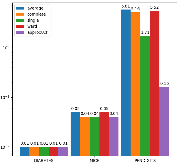
Figure 1: Average running time, in seconds. Logarithmic scale.

References

- [ABF+99] Richa Agarwala, Vineet Bafna, Martin Farach, Mike Paterson, and Mikkel Thorup. On the approximability of numerical taxonomy (fitting distances by tree metrics). SIAM J. Comput., 28(3):1073–1085, 1999.
- [AC11] Nir Ailon and Moses Charikar. Fitting tree metrics: Hierarchical clustering and phylogeny. SIAM J. Comput., 40(5):1275–1291, 2011.
- [ACH19] Amir Abboud, Vincent Cohen-Addad, and Hussein Houdrouge. Subquadratic high-dimensional hierarchical clustering. In Hanna M. Wallach, Hugo Larochelle, Alina Beygelzimer, Florence d’Alché-Buc, Emily B. Fox, and Roman Garnett, editors, Advances in Neural Information Processing Systems 32: Annual Conference on Neural Information Processing Systems 2019, NeurIPS 2019, 8-14 December 2019, Vancouver, BC, Canada, pages 11576–11586, 2019.
- [AI06] Alexandr Andoni and Piotr Indyk. Near-optimal hashing algorithms for approximate nearest neighbor in high dimensions. In 2006 47th annual IEEE symposium on foundations of computer science (FOCS’06), pages 459–468. IEEE, 2006.
- [Alm19] Josh Alman. An illuminating algorithm for the light bulb problem. In 2nd Symposium on Simplicity in Algorithms, SOSA@SODA 2019, January 8-9, 2019 - San Diego, CA, USA, pages 2:1–2:11, 2019.
- [BBV08] Maria-Florina Balcan, Avrim Blum, and Santosh Vempala. A discriminative framework for clustering via similarity functions. In Proceedings of the fortieth annual ACM symposium on Theory of computing, pages 671–680. ACM, 2008.
- [CAKMT17] Vincent Cohen-Addad, Varun Kanade, and Frederik Mallmann-Trenn. Hierarchical clustering beyond the worst-case. In Advances in Neural Information Processing Systems, pages 6201–6209, 2017.
- [CAKMTM18] Vincent Cohen-Addad, Varun Kanade, Frederik Mallmann-Trenn, and Claire Mathieu. Hierarchical clustering: Objective functions and algorithms. In Proceedings of the Twenty-Ninth Annual ACM-SIAM Symposium on Discrete Algorithms, pages 378–397. SIAM, 2018.
- [CC17] Moses Charikar and Vaggos Chatziafratis. Approximate hierarchical clustering via sparsest cut and spreading metrics. In Proceedings of the Twenty-Eighth Annual ACM-SIAM Symposium on Discrete Algorithms, pages 841–854. Society for Industrial and Applied Mathematics, 2017.
- [CCG+98] Moses Charikar, Chandra Chekuri, Ashish Goel, Sudipto Guha, and Serge Plotkin. Approximating a finite metric by a small number of tree metrics. In Proceedings 39th Annual Symposium on Foundations of Computer Science (Cat. No. 98CB36280), pages 379–388. IEEE, 1998.
- [CCN19] Moses Charikar, Vaggos Chatziafratis, and Rad Niazadeh. Hierarchical clustering better than average-linkage. In Proceedings of the Thirtieth Annual ACM-SIAM Symposium on Discrete Algorithms, pages 2291–2304. SIAM, 2019.
- [CCNY18] Moses Charikar, Vaggos Chatziafratis, Rad Niazadeh, and Grigory Yaroslavtsev. Hierarchical clustering for euclidean data. arXiv preprint arXiv:1812.10582, 2018.
- [CIP06] Chris Calabro, Russell Impagliazzo, and Ramamohan Paturi. A duality between clause width and clause density for SAT. In 21st Annual IEEE Conference on Computational Complexity (CCC 2006), 16-20 July 2006, Prague, Czech Republic, pages 252–260, 2006.
- [CM10] Gunnar Carlsson and Facundo Mémoli. Characterization, stability and convergence of hierarchical clustering methods. Journal of machine learning research, 11(Apr):1425–1470, 2010.
- [CM15] Michael Cochez and Hao Mou. Twister tries: Approximate hierarchical agglomerative clustering for average distance in linear time. In Proceedings of the 2015 ACM SIGMOD international conference on Management of data, pages 505–517. ACM, 2015.
- [Das15] Sanjoy Dasgupta. A cost function for similarity-based hierarchical clustering. arXiv preprint arXiv:1510.05043, 2015.
- [DKL19] Roee David, Karthik C. S., and Bundit Laekhanukit. On the complexity of closest pair via polar–pair of point–sets. SIAM J. Discrete Math., 33(1):509–527, 2019.
- [FKW95] Martin Farach, Sampath Kannan, and Tandy J. Warnow. A robust model for finding optimal evolutionary trees. Algorithmica, 13(1/2):155–179, 1995.
- [FN18] Arnold Filtser and Ofer Neiman. Light spanners for high dimensional norms via stochastic decompositions. In 26th Annual European Symposium on Algorithms, ESA 2018, August 20-22, 2018, Helsinki, Finland, pages 29:1–29:15, 2018.
- [GO95] Anka Gajentaan and Mark H. Overmars. On a class of o(n2) problems in computational geometry. Comput. Geom., 5:165–185, 1995.
- [GO12] Anka Gajentaan and Mark H. Overmars. On a class of o(n) problems in computational geometry. Comput. Geom., 45(4):140–152, 2012.
- [HPIS13] Sariel Har-Peled, Piotr Indyk, and Anastasios Sidiropoulos. Euclidean spanners in high dimensions. In Proceedings of the twenty-fourth annual ACM-SIAM symposium on Discrete algorithms, pages 804–809. SIAM, 2013.
- [IP01] Russell Impagliazzo and Ramamohan Paturi. On the complexity of k-sat. Journal of Computer and System Sciences, 62(2):367–375, 2001.
- [IPZ01] Russell Impagliazzo, Ramamohan Paturi, and Francis Zane. Which problems have strongly exponential complexity? Journal of Computer and System Sciences, 63(4):512–530, 2001.
- [KKK16] Matti Karppa, Petteri Kaski, and Jukka Kohonen. A faster subquadratic algorithm for finding outlier correlations. In Proceedings of the Twenty-Seventh Annual ACM-SIAM Symposium on Discrete Algorithms, SODA 2016, Arlington, VA, USA, January 10-12, 2016, pages 1288–1305, 2016.
- [KM19] Karthik C. S. and Pasin Manurangsi. On closest pair in euclidean metric: Monochromatic is as hard as bichromatic. In 10th Innovations in Theoretical Computer Science Conference, ITCS 2019, January 10-12, 2019, San Diego, California, USA, pages 17:1–17:16, 2019.
- [MW17] Benjamin Moseley and Joshua Wang. Approximation bounds for hierarchical clustering: Average linkage, bisecting k-means, and local search. In Advances in Neural Information Processing Systems, pages 3094–3103, 2017.
- [PVG+11] F. Pedregosa, G. Varoquaux, A. Gramfort, V. Michel, B. Thirion, O. Grisel, M. Blondel, P. Prettenhofer, R. Weiss, V. Dubourg, J. Vanderplas, A. Passos, D. Cournapeau, M. Brucher, M. Perrot, and E. Duchesnay. Scikit-learn: Machine learning in Python. Journal of Machine Learning Research, 12:2825–2830, 2011.
- [RP16] Aurko Roy and Sebastian Pokutta. Hierarchical clustering via spreading metrics. In Advances in Neural Information Processing Systems, pages 2316–2324, 2016.
- [Rub18] Aviad Rubinstein. Hardness of approximate nearest neighbor search. In Proceedings of the 50th Annual ACM SIGACT Symposium on Theory of Computing, STOC 2018, Los Angeles, CA, USA, June 25-29, 2018, pages 1260–1268, 2018.
- [RW19] Aviad Rubinstein and Virginia Vassilevska Williams. SETH vs approximation. SIGACT News, 50(4):57–76, 2019.
- [Val88] Leslie G. Valiant. Functionality in neural nets. In Proceedings of the First Annual Workshop on Computational Learning Theory, COLT ’88, Cambridge, MA, USA, August 3-5, 1988, pages 28–39, 1988.
- [Val15] Gregory Valiant. Finding correlations in subquadratic time, with applications to learning parities and the closest pair problem. J. ACM, 62(2):13:1–13:45, 2015.
- [Ver18] Roman Vershynin. High-Dimensional Probability: An Introduction with Applications in Data Science. Cambridge Series in Statistical and Probabilistic Mathematics. Cambridge University Press, 2018.
- [Wil05] Ryan Williams. A new algorithm for optimal 2-constraint satisfaction and its implications. Theor. Comput. Sci., 348(2-3):357–365, 2005.
- [Wil15] Virginia Vassilevska Williams. Hardness of easy problems: Basing hardness on popular conjectures such as the strong exponential time hypothesis (invited talk). In 10th International Symposium on Parameterized and Exact Computation, IPEC 2015, September 16-18, 2015, Patras, Greece, pages 17–29, 2015.
- [Wil16] Virginia Vassilevska Williams. Fine-grained algorithms and complexity (invited talk). In 33rd Symposium on Theoretical Aspects of Computer Science, STACS 2016, February 17-20, 2016, Orléans, France, pages 3:1–3:1, 2016.
- [Wil18] Virginia Vassilevska Williams. On some fine-grained questions in algorithms and complexity. In Proc. Int. Cong. of Math., volume 3, pages 3431–3472, 2018.