A VCG-based Fair Incentive Mechanism for Federated Learning

Abstract

Federated learning (FL) has shown great potential for addressing the challenge of isolated data islands while preserving data privacy. It allows artificial intelligence (AI) models to be trained on locally stored data in a distributed manner. In order to build an ecosystem for FL to operate in a sustainable manner, it has to be economically attractive to data owners. This gives rise to the problem of FL incentive mechanism design, which aims to find the optimal organizational and payment structure for the federation in order to achieve a series of economic objectives. In this paper, we present a VCG-based FL incentive mechanism, named FVCG, specifically designed for incentivizing data owners to contribute all their data and truthfully report their costs in FL settings. It maximizes the social surplus and minimizes unfairness of the federation. We provide an implementation of FVCG with neural networks and theoretic proofs on its performance bounds. Extensive numerical experiment results demonstrated the effectiveness and economic reasonableness of FVCG.

Introduction

In many application scenarios, data are usually segregated into isolated data islands. In addition, due to regulations such as GDPR (?), the requirements on data privacy preservation has become more strict than before. In recent years, federated learning (FL) has emerged as a promising solution for the problem of data fragmentation and privacy preservation, which are important issues hindering the further advancement of artificial intelligence (AI). FL enables data owners to collaboratively train machine learning models in a distributed manner without compromising data privacy (?).

Existing FL platforms such as TensorFlow Federated (TFF) by Google and FATE by WeBank have been developed. Industries such as finance, insurance, telecommunications, healthcare, education, and urban computing are domains that contain application scenarios which can benefit from these platforms. During the process of implementing FL, especially when it involves corporate data owners, many practitioners found it difficult to come up with a reasonable profit distribution plan acceptable to all participating data owners. In some FL platforms such as FATE, the FL model is composed of encrypted sub-models exclusively owned by each data owner (?). It is crucial that all these data owners find it economically attractive to stay in the federation to prevent the FL model from breaking down.

These considerations give rise to the problem of FL incentive mechanism design, formally defined as the problem of finding the optimal organizational and payment structure for the federation in order to achieve desirable operational objectives (?). This problem can be further divided into a demand side problem and a supply side problem, the latter of which decides how many data owners should be included in the federation and how much the federation should pay each data owner.

In this paper, we provide a supply side FL incentive mechanism, named Fair-VCG (FVCG). Based on the famous Vickrey-Clarke-Groves (VCG) mechanism, FVCG promotes fair treatment of FL participants. Economic concepts in FVCG bear clear practical meanings. Therefore, it can be readily engineered into mainstream FL platforms as a standard module. Theoretical analysis shows that FVCG is incentive compatible, individually rational, fair and budget-balanced. Extensive numerical experiment results demonstrated the effectiveness and economic reasonableness of FVCG.

Related Works

The research reported in this paper is interdisciplinary in nature. The proposed FVCG approach is built on the foundation of the following three disciplines.

The first related field is mechanism design. Mechanism design is an important subfield of game theory. It dates back to Hurwicz in 1960 (?). Subsequently, Harsanyi developed the theory of games with incomplete information (?; ?; ?). Hurwicz introduced the notion of incentive compatibility in 1972 (?). Based on these fundamental concepts, the VCG mechanism, which was generalized from Vickrey’s second price auction (?) was proposed (?; ?). This paper has a strong lineage with algorithmic VCG mechanism. Nisan and Ronen (?) studied the computational aspect of VCG mechanisms and introduced VCG into computer science.

The other is the field of federated learning. The concept of FL was first proposed by Google (?; ?; ?) and further developed by WeBank (?). In 2018, WeBank published a white paper (?) to set up a framework of FL. Numerous works followed. In particular, FL incentive mechanism design was formally established as a separate research direction (?; ?), which is further extended by this paper with more formalisms from incentive mechanisms on other related machine learning problems (?; ?).

The last is computational methods of solving functional equations (?; ?; ?; ?). Functional equations are a special type of equations in which the unknowns are functions. Solutions to functional equations are those functions (instead of values of variables) that satisfy the equations for all possible values of the variables. Neural networks have been used to solve functional equations such as Bellman equations (?) and partial differential equations (?). This is possible because neural networks can approximate continuous functions accurately (?; ?).

Problem Formulation

The game theoretic environment for the supply side of the FL incentive mechanism design problem is set up as follows:

• There exists a set of $n$ data owners, denoted by $N=(0,1,\ldots,n-1)$;

• Each data owner $i\in N$ owns some private data with data quality $q_{i}$. Herein data quality bears its generalized meaning so that a bigger data size also results in a larger $q_{i}$. Data quality can be measured based on the marginal contribution to the quality of the federated model by the given dataset. For details, refer to (?).

• Each data owner $i\in N$ has a private cost type $\gamma_{i}$. The higher $\gamma_{i}$indicates a higher cost $c_{i}(q_{i},\gamma_{i})$ for data owner $i$ to contribute data at a given data quality $q_{i}$.

• Data owners report their private data qualities and private cost types to the FL server. In general, there is no guarantee for truthful reporting. The reported data quality and cost type of data owner $i$ are denoted by $\hat{q}_{i}$ and $\hat{\gamma}_{i}$.

• The FL server determines how much data to accept from each data owner, i.e., the acceptance vector $\bm{\eta}(\hat{\bm{q}},\hat{\bm{\gamma}})\in[0,1]^{n}$, as a function of the reported data quality vector $\hat{\bm{q}}$ and the reported cost type vector $\hat{\bm{\gamma}}$, where $\eta_{i}(\cdot)=1$ means data owner $i$ is accepted and $\eta_{i}(\cdot)=0$, rejected. Only accepted data are encrypted and fed to the federated model. The accepted data quality vector $\hat{\bm{q}}\odot\bm{\eta}$ is the Hadamard product of the reported data quality vector and the acceptance vector.

• The trained FL model generates a federation revenue $B(\hat{\bm{q}}\odot\bm{\eta})$, a function of the accepted data quality vector. Note that $B(\cdot)$ is a composite function of $\bar{B}(Q)$, the map from the federated model quality $Q$ to the federation revenue, and $Q(\hat{\bm{q}}\odot\bm{\eta})$, the map from the accepted data quality vector $\hat{\bm{q}}\odot\bm{\eta}$ to the federated model quality, i.e., $B(\cdot)=\bar{B}(Q(\cdot))$.

• The FL server determines the payment vector $\bm{p}(\hat{\bm{q}},\hat{\bm{\gamma}})$, in which $p_{i}(\hat{\bm{q}},\hat{\bm{\gamma}})$ indicates the payment to data owner $i$, as a function of the reported data quality vector $\hat{\bm{q}}$ and the reported cost type vector $\hat{\bm{\gamma}}$.

• Data owner $i$ has preference over different $(p_{i},\eta_{i})$ represented by a quasilinear utility function (?) $u_{i}(\cdot)=p_{i}(\hat{\bm{q}},\hat{\bm{\gamma}})-c_{i}(\hat{q}_{i}\eta_{i},\gamma_{i})$.

• The federation gains the social surplus (?) $S(\cdot)$, defined as the federation revenue minus the total cost of data owners. i.e.,

  $$S(\cdot)=B(\hat{\bm{q}}\odot\bm{\eta})-\sum_{i=0}^{n-1}c_{i}(\hat{q}_{i}\eta_{i},\gamma_{i}).$$ (1)

With these concepts and notations, the problem of supply side FL incentive mechanism design can be formally defined as follows:

Definition 1 (Supply Side FL Incentive Mechanism Design).

The supply side FL incentive mechanism design is to design the optimal functions $\bm{p}(\bm{\hat{q}},\bm{\hat{\gamma}})\,\textrm{and}\,\bm{\eta}(\bm{\hat{q}},\bm{\hat{\gamma}})$, as mappings from the reported data quality vector $\hat{\bm{q}}$ and the reported cost type vector $\hat{\bm{\gamma}}$ to the acceptance vector and the payment vector, given that the federation revenue $B(\cdot)$ is an exogenous function of $\bm{\hat{q}}\odot\bm{\eta}$, in order to achieve some desirable objectives.

FVCG optimizes the following objectives:

• (Dominant Incentive Compatibility, DIC) That all agents truthfully report their data qualities and cost types is in Dominant Strategy Equilibrium.

• (Individual Rationality, IR) No player gets worse off than if he quits the federation, i.e., $u_{i}(\bm{\hat{q}},\bm{\hat{\gamma}},\gamma_{i})\geq 0\textrm{\, for }\forall i$

• (Weak Budget Balance, WBB) For all feasible data quality vectors and cost type vectors, the sum of payments to all data owners is no greater than the federation revenue.

  $$\sum_{i=0}^{n-1}p_{i}(\bm{\hat{q}},\bm{\hat{\gamma}})\leq B(\hat{\bm{q}}\odot\bm{\eta}),\textrm{ \, for }\forall\bm{\hat{q}},\bm{\hat{\gamma}}.$$ (2)

• (Social Surplus Maximization, SSM) The social surplus $S(\cdot)$ is maximized.

• (Fairness) Fairness is attained by minimizing an user defined unfairness function

  $$\textrm{Loss1}=\omega(\bm{p}(\hat{\bm{q}},\hat{\bm{\gamma}}),(\bm{q},\bm{\gamma})).$$ (3)

The Proposed FVCG Approach

In FVCG, the payment vector is further divided into the VCG payment vector $\bm{\tau}$ and the adjustment payment vector $\bm{h}^{\star}+\bm{g}^{\star}$, which can be computed by the following steps.

STEP 1. Compute the data acceptance vector $\bm{\eta}^{\star}$

$\bm{\eta}^{\star}$ is the solution to the following optimization problem:

$$\bm{\eta}^{\star}=\textrm{argmax}_{\bm{\eta}\in[0,1]^{n}}\{B(\hat{\bm{q}}\odot\bm{\eta})-\sum_{i=0}^{n-1}c_{i}(\hat{q}_{i}\eta_{i},\hat{\gamma}_{i})\}.$$ (4)

Note that different $(\hat{\bm{q}},\hat{\bm{\gamma}})$ results in different $\bm{\eta}^{\star}$. Therefore, $\bm{\eta}^{\star}$ is a function of $(\hat{\bm{q}},\hat{\bm{\gamma}})$ and can be denoted as $\bm{\eta}^{\star}(\hat{\bm{q}},\hat{\bm{\gamma}})$. The corresponding social surplus is $S^{\star}(\hat{\bm{q}},\hat{\bm{\gamma}})$.

STEP 2. Compute the VCG payment vector $\bm{\tau}$

With $\bm{\eta}^{\star}$ known, we compute the VCG payment $\tau_{i}$ to data owner $i$ as

$$\tau_{i}=S^{\star}(\hat{\bm{q}},\hat{\bm{\gamma}})-S^{-i\star}(\hat{\bm{q}}^{-i},\hat{\bm{\gamma}}^{-i})+c_{i}(\hat{q}_{i}\eta_{i}^{\star}(\hat{\bm{q}},\hat{\bm{\gamma}}),\hat{\gamma}_{i})$$

$$=[B(\hat{\bm{q}}\odot\bm{\eta}^{\star}(\hat{\bm{q}},\hat{\bm{\gamma}}))-B(\hat{\bm{q}^{-i}}\odot\bm{\eta}^{-i\star}(\hat{\bm{q}^{-i}},\hat{\bm{\gamma}^{-i}}))]$$ (5)

$$-\sum_{k\neq i}[c_{k}(\hat{q}_{k}\eta_{k}^{\star}(\hat{\bm{q}},\hat{\bm{\gamma}}),\hat{\gamma}_{k})-c_{k}(\hat{q}_{k}\eta_{k}^{-i\star}(\hat{\bm{q}}^{-i},\hat{\bm{\gamma}}^{-i}),\hat{\gamma}_{k})],$$

where $(\hat{\bm{q}}^{-i},\hat{\bm{\gamma}}^{-i})$ indicates the reported data quality vector and reported cost type vector when data owner $i$ is excluded, and $\bm{\eta}^{-i\star}$ is the corresponding optimal data acceptance vector. $\bm{\tau}$ is also a function of $(\hat{\bm{q}},\hat{\bm{\gamma}})$, thus denoted by $\bm{\tau}(\hat{\bm{q}},\hat{\bm{\gamma}})$.

STEP 3. Compute the adjustment payment vector $\bm{h}^{\star}+\bm{g}^{\star}$

The adjustment payment to data owner $i$ is

$$h_{i}^{\star}(\hat{\bm{q}}^{-i},\hat{\bm{\gamma}}^{-i})+g_{i}^{\star}(\hat{q}_{i}),$$ (6)

where $h_{i}^{\star}$ is a function of $(\hat{\bm{q}}^{-i},\hat{\bm{\gamma}}^{-i})$ and $g_{i}^{\star}$ is an increasing function of $\hat{q}_{i}$. $\bm{h^{\star}}$ and $\bm{g}^{\star}$ satisfies the following functional optimization equation:

$$\bm{h}^{\star}(\cdot),\bm{g}^{\star}(\cdot)=\textrm{argmin}_{\bm{h}(\cdot),\bm{g}(\cdot)}\{$$

$$\quad\lambda_{1}\omega(\bm{\tau}(\hat{\bm{q}},\hat{\bm{\gamma}})+h_{i}(\hat{\bm{q}}^{-i},\hat{\bm{\gamma}}^{-i})+g_{i}(\hat{q}_{i}),(\hat{\bm{q}},\hat{\bm{\gamma}}))$$

$$+\lambda_{2}\sum_{i=0}^{n-1}\textrm{ReLu}[-(S^{\star}(\hat{\bm{q}},\hat{\bm{\gamma}})-S^{-i\star}(\hat{\bm{q}}^{-i},\hat{\bm{\gamma}}^{-i}))$$

$$\quad-(h_{i}(\hat{\bm{q}}^{-i},\hat{\bm{\gamma}}^{-i})+g_{i}(\hat{q}_{i}))]$$

$$+\lambda_{3}\textrm{ReLu}(\sum_{i=0}^{n-1}[(S^{\star}(\hat{\bm{q}},\hat{\bm{\gamma}})-S^{-i\star}(\hat{\bm{q}}^{-i},\hat{\bm{\gamma}}^{-i}))$$

$$\quad+(h_{i}(\hat{\bm{q}}^{-i},\hat{\bm{\gamma}}^{-i})+g_{i}(\hat{q}_{i}))]-S^{\star}(\hat{\bm{q}},\hat{\bm{\gamma}}))\},$$ (7)

where $\lambda_{1},\lambda_{2},\lambda_{3}$ are three hyper-parameters. We further require that the rule of payment is the same for all data owers (this is also a form of fairness) and set the constraint $h_{i}(\cdot)\equiv h(\cdot)$ and $g_{i}(\cdot)\equiv g(\cdot)$ for all $i=0,\ldots,n-1$.

Analysis

This section proves that FVCG can achieve all the desirable objectives listed before under some reasonable assumptions. Since fairness is guaranteed by Eq. STEP 3. Compute the adjustment payment vector $\bm{h}^{\star}+\bm{g}^{\star}$, below we prove that FVCG satisfies DIC, SSM, IR, and WBB.

Proposition 1 (Dominant Incentive Compatibility).

For every data owner $i$, truthfully reporting his data quality $q_{i}$ and cost type $\gamma_{i}$ is the dominant strategy under FVCG, i.e.,

$$u_{i}((q_{i},\hat{\bm{q}}^{-i}),(\gamma_{i},\hat{\bm{\gamma}}^{-i}))\geq u_{i}((\hat{q}_{i},\hat{\bm{q}}^{-i}),(\hat{\gamma}_{i},\hat{\bm{\gamma}}^{-i})),$$

$$for\quad\forall q_{i},\hat{q}_{i},\hat{\bm{q}}^{-i},\gamma_{i},\hat{\gamma}_{i},\hat{\bm{\gamma}}^{-i}.$$ (8)

Proof.

By the definition of $\bm{\eta}^{\star}(\hat{\bm{q}},\hat{\bm{\gamma}})$ and $S^{\star}(\hat{\bm{q}},\hat{\bm{\gamma}})$,

$$for \,\forall\bm{\eta},\quad S^{\star}((q_{i},\hat{\bm{q}}^{-i}),(\gamma_{i},\hat{\bm{\gamma}}^{-i}))\geq B((q_{i},\hat{\bm{q}}^{-i})\odot\bm{\eta})$$

$$-c_{i}(q_{i}\eta_{i},\gamma_{i})-\sum_{k\neq i}c_{i}(\hat{q}_{k}\eta_{k},\hat{\gamma}_{k}).$$ (9)

In particular, for $\bm{\eta}=(\hat{q}_{i}\eta^{\star}_{i}(\hat{\bm{q}},\hat{\bm{\gamma}})/q_{i},\bm{\eta}^{\star}_{-i}(\hat{\bm{q}},\hat{\bm{\gamma}}))$, Eq. Proof. holds. Also, because data owners cannot report a higher data quality than what they actually own, $q_{i}\geq\hat{q}_{i}$, so $g(q_{i})\geq g(\hat{q}_{i})$. Therefore,

$$S^{\star}((q_{i},\hat{\bm{q}}^{-i}),(\gamma_{i},\hat{\bm{\gamma}}^{-i}))+g(q_{i})$$

$$\geq g(\hat{q}_{i})+B((q_{i},\hat{\bm{q}}^{-i})\odot(\hat{q}_{i}\eta^{\star}_{i}(\hat{\bm{q}},\hat{\bm{\gamma}})/q_{i},\bm{\eta}^{\star}_{-i}(\hat{\bm{q}},\hat{\bm{\gamma}})))$$

$$-\sum_{k\neq i}c_{i}(\hat{q}_{k}\eta^{\star}_{k}(\hat{\bm{q}},\hat{\bm{\gamma}}),\hat{\gamma}_{k})-c_{i}(q_{i}\cdot\hat{q}_{i}\eta^{\star}_{i}(\hat{\bm{q}},\hat{\bm{\gamma}})/q_{i},\gamma_{i})$$

$$=S^{\star}((\hat{q}_{i},\hat{\bm{q}}^{-i}),(\hat{\gamma}_{i},\hat{\bm{\gamma}}^{-i}))+g(\hat{q}_{i}).$$ (10)

Adding $h_{i}(\hat{\bm{q}}^{-i},\hat{\bm{\gamma}}^{-i})-S^{-i\star}(\hat{\bm{q}}^{-i},\hat{\bm{\gamma}}^{-i})$ to both sides of Eq. Proof. and substituting $u_{i}(\cdot)=\tau_{i}(\cdot)+h_{i}(\cdot)+g_{i}(\cdot)-c_{i}(\cdot)=S^{\star}(\cdot)-S^{-i\star}(\cdot)+h_{i}(\cdot)+g_{i}(\cdot)$, we get Eq. 1. Q.E.D. ∎

Proposition 2 (Social Surplus Maximization).

FVCG maximizes the social surplus.

Proof.

Note that variables related to social surplus in Eq. 1 are $\hat{\bm{q}}\odot\bm{\eta}$. Suppose $(\hat{\bm{q}}^{\star\star},\bm{\eta}^{\star\star})$ maximizes Eq. 1, then $(\bm{q},\bar{\bm{\eta}})$ also maximizes Eq. 1, where $\bar{\eta}_{i}=\eta^{\star\star}_{i}*\hat{q}^{\star\star}_{i}/q_{i}\leq\eta^{\star\star}_{i}\in[0,1]$. According to Proposition 1, the social surplus attained by FVCG is $S^{\star}(\bm{q},\bm{\gamma})$. Therefore , we only need to prove that $B(\bm{q}\odot\bar{\bm{\eta}})-\sum_{i=0}^{n-1}c_{i}(q_{i}\bar{\eta}_{i},\gamma_{i})\leq S^{\star}(\bm{q},\bm{\gamma})$. This is guaranteed by the definition of $S^{\star}(\bm{q},\bm{\gamma})$. Q.E.D. ∎

Proposition 3 (Individual Rationality).

Given truthful reporting, individual rationality is satisfied when

$$h_{i}(\bm{q}^{-i},\bm{\gamma}^{-i})+g(q_{i})\geq-[S^{\star}(\bm{q},\bm{\gamma})-S^{-i\star}(\bm{q}^{-i},\bm{\gamma}^{-i})].$$ (11)

Proof.

Given truthful reporting, the utility of data owner $i$ is

$$u_{i}(\bm{q},\bm{\gamma})=p_{i}(\bm{q},\bm{\gamma})-c_{i}(q_{i}\eta_{i}^{\star}(\bm{q},\bm{\gamma}),\gamma_{i})$$ (12)

$$=S^{\star}(\bm{q},\bm{\gamma})-S^{-i\star}(\bm{q}^{-i},\bm{\gamma}^{-i})+h_{i}(\bm{q}^{-i},\bm{\gamma}^{-i})+g(q_{i}).$$

WBB requires $u_{i}(\bm{q},\bm{\gamma})\geq 0$, resulting in the inequality in Eq. 11. Q.E.D. ∎

Proposition 4 (Weak Budget Balance).

Given truthful reporting, weak budget balance is satisfied when

$$\sum_{i=0}^{n-1} [h_{i}(\bm{q}^{-i},\bm{\gamma}^{-i})+g(q_{i})]$$

$$\leq S^{\star}(\bm{q},\bm{\gamma})-\sum_{i=0}^{n-1}[S^{\star}(\bm{q},\bm{\gamma})-S^{-i\star}(\bm{q}^{-i},\bm{\gamma}^{-i})].$$ (13)

Proof.

Given truthful reporting, the total payment to all data owners is

$$\sum_{i=0}^{n-1}p_{i}(\bm{q},\bm{\gamma})=\sum_{i=0}^{n-1}[\tau_{i}(\bm{q},\bm{\gamma})+h_{i}(\bm{q}^{-i},\bm{\gamma}^{-i})+g(q_{i})]$$

$$=\sum_{i=0}^{n-1}[S^{\star}(\bm{q},\bm{\gamma})-S^{-i\star}(\bm{q}^{-i},\bm{\gamma}^{-i})+c_{i}(q_{i}\eta_{i}^{\star}(\bm{q},\bm{\gamma}),\gamma_{i})$$

$$+h_{i}(\bm{q}^{-i},\bm{\gamma}^{-i})+g(q_{i})].$$ (14)

WBB requires $\sum_{i=0}^{n-1}p_{i}(\bm{q},\bm{\gamma})\leq B(\bm{q}\odot\bm{\eta}^{\star}(\bm{q},\bm{\gamma}))$. This fact, together with the definition of $S^{\star}(\bm{q},\bm{\gamma})$, leads to the inequality in Eq. 4. Q.E.D. ∎

In prior, the true values of $(\bm{q},\bm{\gamma})$ are unknown, In order that at least one set of $\bm{h}(\cdot)$ and $\bm{g}(\cdot)$ satisfies IR and WBB for all possible $(\bm{q},\bm{\gamma})$, the following theorem holds.

Theorem 1.

The following inequality is the sufficient and necessary condition for the existence of $\bm{h}(\cdot)$ and $\bm{g}(\cdot)$ that allow IR and WBB to hold universally for all possible $(\bm{q},\bm{\gamma})$:

$$\sum_{i=0}^{n-1}[S^{\star}(\bm{q},\bm{\gamma})-S^{\star}((\min q_{i},\bm{q}^{-i}),(\max\gamma_{i},\bm{\gamma}^{-i}))]$$

$$\leq S^{\star}(\bm{q},\bm{\gamma}),\quad for\,\forall\bm{q},\bm{\gamma}.$$ (15)

In order to prove Theorem 1, we prove the following lemmas first.

Lemma 1.

The maximum social surplus is monotonically increasing with $q_{i}$ and monotonically decreasing with $\gamma_{i}$ for every data owner $i$.

Proof.

Similar to the proof of Proposition 2, increasing $q_{i}$ does not hurt the maximal social surplus because we can at least guarantee the same maximal social surplus by adjusting $\eta_{i}$. Therefore, $S^{\star}(\bm{q},\bm{\gamma})$ increases with $q_{i}$.

That $S^{\star}(\bm{q},\bm{\gamma})$ decreases with $\gamma_{i}$ is due to the envelope theorem, which results in

$$\frac{\partial S^{\star}}{\partial\gamma_{i}}|_{\bm{\eta}=\eta^{\star}}=\frac{\partial S}{\partial\gamma_{i}}|_{\bm{\eta}=\eta^{\star}}=-\frac{\partial c_{i}}{\partial\gamma_{i}}|_{\bm{\eta}=\eta^{\star}}\leq 0.$$ (16)

Q.E.D. ∎

Lemma 2.

For $\forall\bm{q},\bm{\gamma}$, $S^{\star}(\bm{q},\bm{\gamma})\geq S^{-i\star}(\bm{q}^{-i},\bm{\gamma}^{-i})$.

Proof.

From Lemma 1, for $\forall\bm{q},\bm{\gamma}$,

$$S^{\star}(\bm{q},\bm{\gamma})\geq S^{\star}((0,\bm{q}^{-i}),(\gamma_{i},\bm{\gamma}^{-i}))=S^{-i\star}(\bm{q}^{-i},\bm{\gamma}^{-i}).$$ (17)

Q.E.D. ∎

Now we can prove Theorem 1 as follows.

Proof of Theorem 1.

Since the left side of Eq. 11 is independent of $\gamma_{i}$ and increases with $q_{i}$, while the right side decreases with $q_{i}$, a sufficient and necessary condition for Eq. 11 to hold is

$$h_{i}(\bm{q}^{-i},\bm{\gamma}^{-i})+g(q_{i})\geq-\min[S^{\star}(\bm{q},\bm{\gamma})-S^{-i\star}(\bm{q}^{-i},\bm{\gamma}^{-i})]$$

$$=-[S^{\star}((\min q_{i},\bm{q}^{-i}),(\max\gamma_{i},\bm{\gamma}^{-i}))-S^{-i\star}(\bm{q}^{-i},\bm{\gamma}^{-i})].$$ (18)

Eq. Proof of Theorem 1., together with Eq. 4, results in Eq. 1.

To prove sufficiency, note that if Eq. 1 holds, $g(q_{i})\equiv 0$ and $h_{i}(\bm{q}^{-i},\bm{\gamma}^{-i})\equiv-[S^{\star}((\min q_{i},\bm{q}^{-i}),(\max\gamma_{i},\bm{\gamma}^{-i}))-S^{-i\star}(\bm{q}^{-i},\bm{\gamma}^{-i})]$ are one set of solution. Q.E.D. ∎

From Theorem 1, we have the following corollary.

Corollary 1.

WBB and IR hold universally for some $\bm{h}(\cdot)$ and $\bm{g}(\cdot)$ if the prior estimation of $(\bm{q},\bm{\gamma})$ is accurate enough.

Proof.

When the the prior estimation of $(\bm{q},\bm{\gamma})$ is accurate enough, the left side of Eq. 1 approaches $0$ while the right side approaches a positive number. Q.E.D. ∎

For those cases when Eq. 1 may not be guaranteed, we minimize the difference between the left side and the right side of Eq. 11 and Eq. 4 when they are violated. Formally, we minimize the following two terms.

$$\textrm{Loss2}=\sum_{i=0}^{n-1}\textrm{ReLu}[-(S^{\star}(\bm{q},\bm{\gamma})-S^{-i\star}(\bm{q}^{-i},\bm{\gamma}^{-i}))$$

$$\quad\quad-(h_{i}(\bm{q}^{-i},\bm{\gamma}^{-i})+g(q_{i}))],$$ (19)

$$\textrm{and}\quad\textrm{Loss3}=\textrm{ReLu}[\sum_{i=0}^{n-1}[(S^{\star}(\bm{q},\bm{\gamma})-S^{-i\star}(\bm{q}^{-i},\bm{\gamma}^{-i}))$$

$$\quad\quad+(h_{i}(\bm{q}^{-i},\bm{\gamma}^{-i})+g(q_{i}))]-S^{\star}(\bm{q},\bm{\gamma})].$$ (20)

Combining Eq. Analysis, Analysis with the unfairness minimization requirement in Eq. 3, we set the loss function of FVCG as that in Eq. STEP 3. Compute the adjustment payment vector $\bm{h}^{\star}+\bm{g}^{\star}$. The hyper-parameters $\lambda_{1},\lambda_{2},\lambda_{3}$ represent the relative importance put on fairness, IR and WBB.

The Computational Solution

Neural Network for Functional Optimization

The optimization problem in Eq. STEP 3. Compute the adjustment payment vector $\bm{h}^{\star}+\bm{g}^{\star}$ is a functional equation. While there is no general method for deriving analytical solutions to functional equations, we can use neural networks to approximate $\bm{h}^{\star}(\cdot)$ and $\bm{g}^{\star}(\cdot)$. Neural networks are feasible functional optimization methods because they can approximate continuous functions to arbitrary precisions (?). Neural networks with non-negative weights, called monotonic networks, can approximate continuous and increasing functions to arbitrary precisions (?).

The FVCG Neural Network

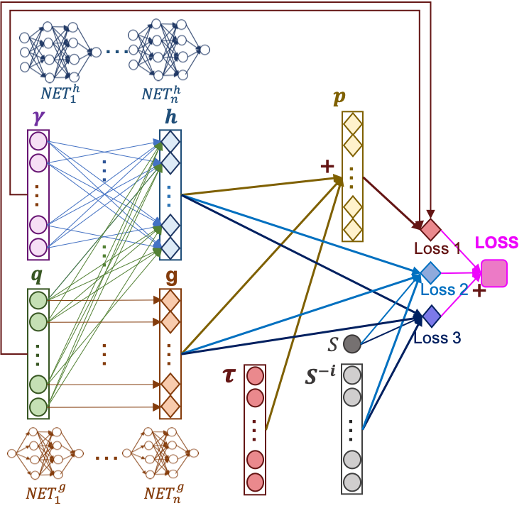
Figure 1: The structure of the composite neural network of FVCG

In order to solve the functional optimization problem of FVCG in Eq. STEP 3. Compute the adjustment payment vector $\bm{h}^{\star}+\bm{g}^{\star}$, we construct $n$ neural networks $\textrm{NET}^{h}_{i},i=0,\ldots,n-1$ which share the same set of parameters to approximate $h_{i}(\cdot),i=0,\ldots,n-1$, and another $n$ monotonic networks $\textrm{NET}^{g}_{i},i=0,\ldots,n-1$ sharing another set of parameters to approximate $g_{i}(\cdot),i=0,\ldots,n-1$. The output layer of $\textrm{NET}^{g}_{i}$ has no bias in order to avoid the multicollinearity problem involved in adding up $\textrm{NET}^{h}_{i}$ and $\textrm{NET}^{g}_{i}$.

Then, we combine the output nodes of these $2n$ networks into a single composite neural network with the following loss function.

$$\textrm{LOSS}=\frac{1}{T}\sum_{t=0}^{T-1}\{$$

$$\lambda_{1}\omega(\bm{\tau}(\bm{q}^{t},\bm{\gamma}^{t})+\textrm{NET}^{h}_{i}(\bm{q}^{-i,t},\bm{\gamma}^{-i,t})+\textrm{NET}^{g}_{i}(q^{t}_{i}),(\bm{q}^{t},\bm{\gamma}^{t}))$$

$$+\lambda_{2}\sum_{i=0}^{n-1}\textrm{ReLu}[-(S^{\star}(\bm{q}^{t},\bm{\gamma}^{t})-S^{-i\star}(\bm{q}^{-i,t},\bm{\gamma}^{-i,t}))$$

$$\quad-(\textrm{NET}^{h}_{i}(\bm{q}^{-i,t},\bm{\gamma}^{-i,t})+\textrm{NET}^{g}_{i}(q^{t}_{i}))]$$

$$+\lambda_{3}\textrm{ReLu}(\sum_{i=0}^{n-1}[(S^{\star}(\bm{q}^{t},\bm{\gamma}^{t})-S^{-i\star}(\bm{q}^{-i,t},\bm{\gamma}^{-i,t}))$$ (21)

$$\quad+(\textrm{NET}^{h}_{i}(\bm{q}^{-i,t},\bm{\gamma}^{-i,t})+\textrm{NET}^{g}_{i}(q^{t}_{i}))]-S^{\star}(\bm{q}^{t},\bm{\gamma}^{t}))\},$$

where $(\bm{q}^{t},\bm{\gamma}^{t}),t=0,\ldots,T-1$ are randomly generated data points drawn from the prior belief on the distribution of $(\bm{q},\bm{\gamma})$, denoted By $\Delta(\bm{q})$ and $\Delta(\bm{\gamma})$.

Fig. 1 is an illustration of the composite neural network constructed. The circles represent input nodes of this neural network. Note that $2n$ small networks constitute this composite neural network. Training this composite network results in the optimal weights for $[\textrm{NET}^{h}_{i}],[\textrm{NET}^{g}_{i}]$.

Training

Algorithm 1 Train $[\textrm{NET}^{h}_{i}],[\textrm{NET}^{g}_{i}]$ for all $i$

0:  Neural networks: $[\textrm{NET}^{h}_{i}],[\textrm{NET}^{g}_{i}]$. Probability Distribution: $\Delta(\bm{q})$ , $\Delta(\bm{\gamma})$

0:  Trained networks: $[\textrm{NET}^{h}_{i}],[\textrm{NET}^{g}_{i}]$

1:  construct the composite neural network for LOSS where input nodes are those in Eq. 22 and the LOSS node is constructed according to Eq. The FVCG Neural Network

2:  $\textrm{PAR}\leftarrow$ list of all parameters of the computation graph

3:  initialize PAR

4:  for $l$ in range($iterations$) do

5:     for $t$ in range($T$) do

6:        randomly draw $(\bm{q}^{t},\bm{\gamma}^{t})$ from $\Delta(\bm{q}),\Delta(\bm{\gamma})$

7:        compute $\bm{\tau}^{t}$, $S^{\star,t}$ and all $S^{-i\star,t}$

8:     end for

9:     assign $(\bm{q}^{t},\bm{\gamma}^{t}),\bm{\tau}^{t},S^{-i\star,t},S^{\star,t},i=0,\ldots,n-1,t=1,\ldots,S$ to corresponding input nodes of LOSS.

10:     feedForward(LOSS)

11:     backPropogation(LOSS)

12:     $\delta\leftarrow$ $(\frac{d\textrm{LOSS}}{d\textrm{PAR}}).value$

13:     PAR$.value\leftarrow\textrm{PAR}.value-a*\delta$

14:     if  exist $\tau^{t}_{i}+\textrm{NET}^{h,t}_{i}.value+\textrm{NET}^{g,t}_{i}.value<0$ then

15:        increase the bias of the output layer of $\textrm{NET}^{h}_{i}$ by $b$

16:     end if

17:  end for

The training procedure for FVCG is described in Algorithm 1. Within this algorithm, CAPITALIZED words refer to nodes in the composite neural network, whereas lowercased words stand for other types of variables. The value of a node is referenced as NODE.$value$. The composite neural network is constructed according to Eq. The FVCG Neural Network, where the following variables are fed to the input nodes:

$$(\bm{q}^{t},\bm{\gamma}^{t}),\bm{\tau}^{t},S^{-i\star,t},S^{\star,t},i=0,\ldots,n-1,t=0,\ldots,T-1.$$ (22)

In Algorithm 1, PAR is the collection of nodes of all trainable variables in the computation graph of LOSS. We carry out the backpropagation and gradient decent on PAR in each iteration in order to reduce the value of LOSS. Since payments to data owners cannot be negative, we increase the bias of the output layer of $\textrm{NET}^{h}_{i}$ by a positive number $b$ if some payments are negative.

Algorithm 1 is unsupervised learning in nature and no labelling is required. Furthermore, we do not need any real training data because the purpose of Algorithm 1 is to learn the optimal functions $\bm{h}(\cdot)$ and $\bm{g}(\cdot)$ that minimize the expected value of LOSS for random $(\bm{q},\bm{\gamma})$. We only need to guarantee that $(\bm{q},\bm{\gamma})$ is randomly drawn from the prior probability distribution $(\Delta(\bm{q}),\Delta(\bm{\gamma}))$. Therefore, training data in Algorithm 1 are randomly generated. A different set of training data of size $T$ is generated for each iteration, where $T$ plays a role similar to that of the batch size in other neural network trainings. $T$ does not need to be very large.

Experimental Evaluation

In real application scenarios of FVCG, the federation revenue function $B(\cdot)$ is estimated from the real economic performance of the trained federated model. That requires a separate functional module in the FL server to evaluate each data owner’s contribution to the federated model and, in turn, the increment of the federation revenue. The individual cost function $c_{i}(\cdot)$ is estimated from market surveys. On the other hand, the unfairness function $\omega(\cdot)$ is subjectively specified by the FM system designer.

Real $B(\cdot)$ and $c_{i}(\cdot)$ depend on economic behaviors of human beings in the real market environment. It requires advanced econometric techniques to choose the proper functional forms for $B(\cdot)$ and $c_{i}(\cdot)$ (similar problems discussed by (?; ?; ?; ?; ?)), which is an equally complex problem and is beyond the scope of this paper. Similarly, estimating the prior beliefs $\Delta(\bm{q})$ and $\Delta(\bm{\gamma})$ also requires professional market analysis techniques. At the moment, we only carry out experiments based on hypothetical functional forms of $B(\cdot)$, $c_{i}(\cdot)$, and hypothetical prior beliefs $\Delta(\bm{q})$, $\Delta(\bm{\gamma})$. With these hypothetical specifications, we evaluate the performance of FVCG under various conditions through simulations. Although the results of this experiment cannot be applied to real scenarios, they are enough for revealing the reasonableness of FVCG and our neural network-based method.

Experiment Settings

In our experiment, we specify the revenue function, the cost function and the unfairness function as follows:

$$B(\bm{q}\odot\bm{\eta})=\alpha\sqrt{\sum_{i=0}^{n-1}q_{i}\eta_{i}},$$ (23)

$$c_{i}(q_{i}\eta_{i},\gamma_{i})=\gamma_{i}q_{i}\eta_{i},i=0,\ldots,n-1,$$ (24)

$$\omega(\bm{p}(\bm{q},\bm{\gamma}),(\bm{q},\bm{\gamma}))= \frac{1}{n}\sum_{i=0}^{n-1}(\frac{q_{i}}{q_{i}+p_{i}(\bm{q},\bm{\gamma})})^{2}$$

$$-[\frac{1}{n}\sum_{i=0}^{n-1}(\frac{q_{i}}{q_{i}+p_{i}(\bm{q},\bm{\gamma})})]^{2}.$$ (25)

Note that unfairness under such a definition reaches $0$ when the unit price of data quality is the same for all data owners.

Algorithm 2 Calculate $\bm{\eta}^{\star}$ and $S^{\star}$

0:  Inputs: $\bm{q},\bm{\gamma}$.

0:  $S^{\star}=\alpha\sqrt{\sum_{i=0}^{n-1}q_{i}\eta^{\star}_{i}}-\sum_{i=0}^{n-1}\gamma_{i}q_{i}\eta^{\star}_{i}$$\bm{\eta}^{\star}=\textrm{argmax}_{\bm{\eta}\in[0,1]^{n}}\{\alpha\sqrt{\sum_{i=0}^{n-1}q_{i}\eta_{i}}-\sum_{i=0}^{n-1}\gamma_{i}q_{i}\eta_{i}\}$

1:  $[\gamma^{(j)}]\leftarrow$ $[\gamma_{i}]$ sorted in increasing order

2:  index $\leftarrow$ a list of integers, s.t. $\gamma^{(j)}=\gamma_{\textrm{index}[j]}$

3:  for $j$ in range$(n)$ do

4:     if $\frac{\alpha}{2\sqrt{\sum_{l=0}^{j}q_{\textrm{index}(l)}}}\geq\gamma^{(j)}$ then

5:        $\eta^{\star}_{\textrm{index}(j)}\leftarrow 1$

6:     else if $j\neq 1$ and $\frac{\alpha}{2\sqrt{\sum_{l=0}^{j-1}q_{\textrm{index}(l)}}}\leq\gamma^{(j)}$ then

7:        $\eta^{\star}_{\textrm{index}(j)}\leftarrow 0$

8:     else

9:        $\eta^{\star}_{\textrm{index}(j)}\leftarrow\frac{(\alpha/(2\gamma^{(j)}))^{2}-\sum_{l=0}^{j-1}q_{\textrm{index}(l)}}{q_{\textrm{index}(j)}}$

10:     end if

11:  end for

12:  $S^{\star}\leftarrow\alpha\sqrt{\sum_{i=0}^{n-1}q_{i}\eta^{\star}_{i}}-\sum_{i=0}^{n-1}\gamma_{i}q_{i}\eta^{\star}_{i}$

Under the above specification, we can explicitly solve $\bm{\eta}^{\star}$ and $S^{\star}$ according to Algorithm 2. $S^{-i\star}$ can also be calculated from Algorithm 2 by taking $\bm{q}^{-i},\bm{\gamma}^{-i}$ as inputs. Then $\bm{\tau}$ can be computed from Eq. STEP 2. Compute the VCG payment vector $\bm{\tau}$. After computing $\bm{\tau}$, $S^{\star}$ and $S^{-i\star}$, we can apply Algorithm 1 to train $[\textrm{NET}^{h}_{i}],[\textrm{NET}^{g}_{i}]$.

Experiment Results

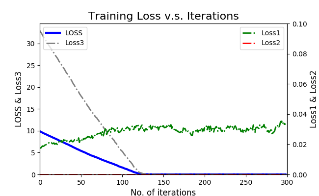
Figure 2: Training loss v.s. iterations

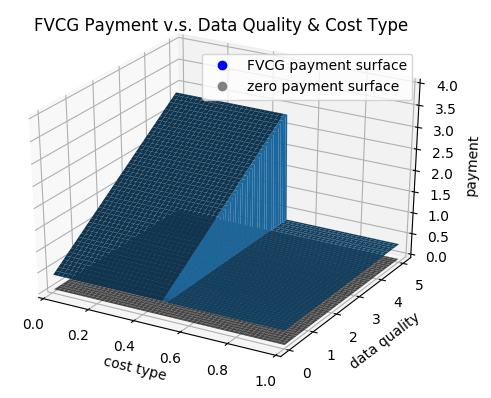
Figure 3: Payment to data owner v.s. data quality & cost type

Table 1: Payments to data owners when their data qualities are the same

	data quality (same for all data owners)
cost type	$q_{i}=\bm{1.0}$ for $\forall i$				$q_{i}=\bm{2.0}$ for $\forall i$				$q_{i}=\bm{3.0}$ for $\forall i$				$q_{i}=\bm{4.0}$ for $\forall i$
(different)	$p_{i}$	$\eta_{i}$	$\tau_{i}$	$h_{i}+g_{i}$	$p_{i}$	$\eta_{i}$	$\tau_{i}$	$h_{i}+g_{i}$	$p_{i}$	$\eta_{i}$	$\tau_{i}$	$h_{i}+g_{i}$	$p_{i}$	$\eta_{i}$	$\tau_{i}$	$h_{i}+g_{i}$
0.1	1.01	1.00	0.67	0.3362	1.40	1.00	1.06	0.3465	1.81	1.00	1.45	0.3552	2.06	1.00	1.70	0.3623
0.2	1.01	1.00	0.67	0.3366	1.40	1.00	1.06	0.3468	1.81	1.00	1.45	0.3554	2.06	1.00	1.70	0.3624
0.3	1.01	1.00	0.67	0.3371	1.40	1.00	1.06	0.3472	1.81	1.00	1.45	0.3557	2.06	1.00	1.70	0.3626
0.4	1.01	1.00	0.67	0.3365	1.40	1.00	1.06	0.3467	1.81	1.00	1.45	0.3553	1.91	0.91	1.55	0.3623
0.5	1.01	1.00	0.67	0.3369	1.40	1.00	1.06	0.3470	0.36	0.00	0.00	0.3555	0.36	0.00	0.00	0.3625
0.6	1.01	1.00	0.67	0.3358	0.35	0.00	0.00	0.3460	0.35	0.00	0.00	0.3547	0.36	0.00	0.00	0.3619
0.7	0.34	0.00	0.00	0.3363	0.35	0.00	0.00	0.3464	0.35	0.00	0.00	0.3550	0.36	0.00	0.00	0.3620
0.8	0.34	0.00	0.00	0.3356	0.35	0.00	0.00	0.3457	0.35	0.00	0.00	0.3544	0.36	0.00	0.00	0.3616
0.9	0.34	0.00	0.00	0.3350	0.35	0.00	0.00	0.3453	0.35	0.00	0.00	0.3541	0.36	0.00	0.00	0.3614
1.0	0.34	0.00	0.00	0.3359	0.35	0.00	0.00	0.3460	0.35	0.00	0.00	0.3547	0.36	0.00	0.00	0.3618
Loss1	0.0152				0.0175				0.0176				0.0153
Loss2	0.0000				0.0000				0.0000				0.0000
Loss3	0.0000				0.0000				0.0000				0.0000
LOSS	0.0061				0.0070				0.0070				0.0061

Table 2: Payments to data owners when their cost types are the same

	cost type (same for all data owners)
data quality	$\gamma_{i}=\bm{0.2}$ for $\forall i$				$\gamma_{i}=\bm{0.4}$ for $\forall i$				$\gamma_{i}=\bm{0.6}$ for $\forall i$				$\gamma_{i}=\bm{0.8}$ for $\forall i$
(different)	$p_{i}$	$\eta_{i}$	$\tau_{i}$	$h_{i}+g_{i}$	$p_{i}$	$\eta_{i}$	$\tau_{i}$	$h_{i}+g_{i}$	$p_{i}$	$\eta_{i}$	$\tau_{i}$	$h_{i}+g_{i}$	$p_{i}$	$\eta_{i}$	$\tau_{i}$	$h_{i}+g_{i}$
0.5	0.49	1.00	0.15	0.3401	0.54	1.00	0.20	0.3407	0.64	1.00	0.30	0.3414	0.74	1.00	0.40	0.3420
1.0	0.65	1.00	0.30	0.3427	0.74	1.00	0.40	0.3433	0.94	1.00	0.60	0.3440	1.14	1.00	0.80	0.3446
1.5	0.80	1.00	0.46	0.3455	0.95	1.00	0.60	0.3460	1.25	1.00	0.90	0.3466	1.55	1.00	1.20	0.3472
2.0	0.96	1.00	0.61	0.3472	1.15	1.00	0.80	0.3477	1.55	1.00	1.20	0.3482	1.07	0.45	0.73	0.3487
2.5	1.12	1.00	0.77	0.3489	1.35	1.00	1.00	0.3493	1.52	0.78	1.17	0.3496	0.35	0.00	0.00	0.3501
3.0	1.28	1.00	0.93	0.3513	1.55	1.00	1.20	0.3518	0.35	0.00	0.00	0.3522	0.35	0.00	0.00	0.3526
3.5	1.45	1.00	1.09	0.3550	1.76	1.00	1.40	0.3556	0.36	0.00	0.00	0.3561	0.36	0.00	0.00	0.3566
4.0	1.61	1.00	1.25	0.3573	1.01	0.41	0.65	0.3577	0.36	0.00	0.00	0.3581	0.36	0.00	0.00	0.3585
4.5	1.78	1.00	1.42	0.3606	0.36	0.00	0.00	0.3611	0.36	0.00	0.00	0.3616	0.36	0.00	0.00	0.3621
5.0	1.94	1.00	1.58	0.3616	0.36	0.00	0.00	0.3622	0.36	0.00	0.00	0.3628	0.36	0.00	0.00	0.3634
Loss1	0.0041				0.0196				0.0378				0.0432
Loss2	0.0000				0.0000				0.0000				0.0000
Loss3	0.0000				0.0000				0.0000				0.4009
LOSS	0.0016				0.0078				0.0151				0.1375

Here, we report the experiment results for $n=10,\alpha=\sqrt{n}$. We set $\Delta(q_{i})$, the prior belief on data quality $q_{i}$ to be a uniform distribution on $[0,5]$, and $\Delta(\gamma_{i})$ a uniform distribution on $[0,1]$. We set the the hyper-parameters to be $\lambda_{1}=0.4,\lambda_{2}=0.3,\lambda_{3}=0.3,T=100,a=0.001,b=1.0$, and $\textrm{NET}^{h}_{i}$, $\textrm{NET}^{g}_{i}$ to have three $10$-dimension hidden layers and one $50$-dimension hidden layer, respectively.

The training loss converges after $120$ iterations, as is shown in Fig. 2. We also report the three components of LOSS, i.e., Loss1, Loss2, and Loss3, reflecting the unfairness level, the IR condition, and WBB, respectively.

After we obtain the trained networks $[\textrm{NET}^{h}_{i}],[\textrm{NET}^{g}_{i}],i=0,1,...n-1$, we get the payment function $\bm{p}(\bm{q},\bm{\gamma})$. For illustration, we draw $p_{0}$, the payment to data owner $0$ with respect to $q_{0}$ and $\gamma_{0}$ in Fig. 3, fixing parameters of other data owners at $q_{i}\equiv 2.5,\gamma_{i}\equiv 0.5$ for $i\neq 0$.

Also, in Table 2, we list payments to all data owners when they have the same data quality (being $q_{i}=1.0,2.0,3.0,4.0$ for $\forall i$) but different cost types (being $0.1,\ldots,1.0$ for each data owner respectively) in Table 1, and payments when they report the same cost type (being $\gamma_{i}=0.2,0.4,0.6,0.8$ for $\forall i$) but different data qualities (being $0.05,\ldots,0.50$ for each data owner respectively). We also report the intermediate results of $\eta_{i},\tau_{i},h_{i}+g_{i}$ and the losses for each scenario.

Discussions

Note that in Fig. 2, Loss2, reflecting the IR condition, remains $0$ throughout the whole training process. The training LOSS is dominated by Loss3, which is high at the begining and approaches $0$ later. This means that WBB is satisfied by the trained network except for some rare cases. For example, in Table 2, except for the rare case where the cost types of all data owners exceed a threshold (with a prior probability less than $10^{-2}$), Loss3 is $0$. On the other hand, Loss1, the unfairness level, remains positive. This is because by definition the unfairness function being $0$ implies a linear payment structure, which cannot satisfy IR and WBB.

We can see from Fig. 3 that $p_{0}$ is increases with $q_{0}$. This aligns well with our expectation that the more data that a data owner owns and reports, the higher the payment he receives. On the other hand, $p_{0}$ remains constant with $\gamma_{0}$ when $\gamma_{0}$ is not too high, then sharply drops to a smaller constant level beyond a certain threshold. This reflects the fact that if the cost of contributing data is too high for a data owner, it is beneficial to both the federation and the data owner that the federation rejects his data but still pays him a small amount of award for participation.

Such a two-part payment structure is also revealed in Table 1 and Table 2. We can see that if data owner $i$’s cost type is high, $\eta_{i}$ becomes $0$. Data owners with equal cost types are included on a first-come-first-accepted basis. The binary nature of $\eta_{i}$ leads to the two-part structure of $\tau_{i}$ and $p_{i}$. On the other hand, the payment adjustment term, $h_{i}+g_{i}$, is relatively smooth. It increases with $q_{i}$ but is not very sensitive to $\gamma_{i}$. This is because $\bm{\gamma}$ is not included in the unfairness function in the specification of our experiment.

Conclusions and Future Work

In this paper, we presented the Fair-VCG (FVCG) mechanism for optimally sharing revenues with data owners in FL. FVCG incentivizes data owners to contribute all their data and truthfully report their costs. It is individually rational, weakly budget balance, maximizes social surplus while minimizing unfairness. We developed a neural network method to solve the functional optimization problem in FVCG.

In subsequent research, we plan to work out more FL incentive mechanisms optimized for other sets of objectives, compare different mechanisms, and combine them into one single platform. We will also dig deeper into some important details such as identifying the federation revenue function and individual cost functions, reducing information asymmetry and providing advices on optimal strategies for data owners to enable FVCG to perform better in practice.

References

- [Beidokhti and Malek 2009] Beidokhti, R. S., and Malek, A. 2009. Solving initial-boundary value problems for systems of partial differential equations using neural networks and optimization techniques. Journal of the Franklin Institute 346(9):898–913.
- [Boulding 1945] Boulding, K. E. 1945. The concept of economic surplus. The American Economic Review 35(5):851–869.
- [Clarke 1971] Clarke, E. H. 1971. Multipart pricing of public goods. Public choice 11(1):17–33.
- [Coelli 1996] Coelli, T. J. 1996. A guide to frontier version 4.1: a computer program for stochastic frontier production and cost function estimation. Technical report, CEPA Working papers.
- [Cong et al. 2019] Cong, M.; Weng, X.; Yu, H.; and Qu, Z. 2019. Fml incentive mechanism design: Concepts, basic settings, and taxonomy. the 1st International Workshop on Federated Machine Learning for User Privacy and Data Confidentiality.
- [Dekel, Fischer, and Procaccia 2010] Dekel, O.; Fischer, F.; and Procaccia, A. D. 2010. Incentive compatible regression learning. Journal of Computer and System Sciences 76(8):759–777.
- [Diewert 1974] Diewert, W. E. 1974. Functional forms for revenue and factor requirements functions. International Economic Review 119–130.
- [Efthimiou 2011] Efthimiou, C. 2011. Introduction to functional equations: theory and problem-solving strategies for mathematical competitions and beyond, volume 6. American Mathematical Soc.
- [EU 2016] EU. 2016. Regulation (eu) 2016/679 of the european parliament and of the council of 27 april 2016 on the protection of natural persons with regard to the processing of personal data and on the free movement of such data, and repealing directive 95/46. Official Journal of the European Union (OJ) 59(1-88):294.
- [Figlio 1999] Figlio, D. N. 1999. Functional form and the estimated effects of school resources. Economics of education review 18(2):241–252.
- [Funahashi 1989] Funahashi, K.-I. 1989. On the approximate realization of continuous mappings by neural networks. Neural networks 2(3):183–192.
- [Groves and others 1973] Groves, T., et al. 1973. Incentives in teams. Econometrica 41(4):617–631.
- [Halvorsen and Pollakowski 1981] Halvorsen, R., and Pollakowski, H. O. 1981. Choice of functional form for hedonic price equations. Journal of urban economics 10(1):37–49.
- [Harsanyi 1967] Harsanyi, J. C. 1967. Games with incomplete information played by “bayesian” players, part i. the basic model. Management science 14(3):159–182.
- [Harsanyi 1968a] Harsanyi, J. C. 1968a. Games with incomplete information played by “bayesian” players part ii. bayesian equilibrium points. Management Science 14(5):320–334.
- [Harsanyi 1968b] Harsanyi, J. C. 1968b. Games with incomplete information played by “bayesian” players part iii. the basic probability distribution of the game. Management Science 14(5):486–502.
- [Hurwicz 1960] Hurwicz, L. 1960. Optimality and informational efficiency in resource allocation processes. Mathematical methods in the social sciences.
- [Hurwicz 1972] Hurwicz, L. 1972. On informationally decentralized systems. Decision and Organization: A Volume in Honor of J. Marschak.
- [Kannappan 2009] Kannappan, P. 2009. Functional equations and inequalities with applications. Springer Science & Business Media.
- [Konečnỳ et al. 2016a] Konečnỳ, J.; McMahan, H. B.; Ramage, D.; and Richtárik, P. 2016a. Federated optimization: Distributed machine learning for on-device intelligence. arXiv preprint arXiv:1610.02527.
- [Konečnỳ et al. 2016b] Konečnỳ, J.; McMahan, H. B.; Yu, F. X.; Richtárik, P.; Suresh, A. T.; and Bacon, D. 2016b. Federated learning: Strategies for improving communication efficiency. arXiv preprint arXiv:1610.05492.
- [Kuczma 2009] Kuczma, M. 2009. An introduction to the theory of functional equations and inequalities: Cauchy’s equation and Jensen’s inequality. Springer Science & Business Media.
- [McMahan et al. 2016] McMahan, H. B.; Moore, E.; Ramage, D.; Hampson, S.; et al. 2016. Communication-efficient learning of deep networks from decentralized data. arXiv preprint arXiv:1602.05629.
- [Meir, Procaccia, and Rosenschein 2012] Meir, R.; Procaccia, A. D.; and Rosenschein, J. S. 2012. Algorithms for strategyproof classification. Artificial Intelligence 186:123–156.
- [Munos, Baird, and Moore 1999] Munos, R.; Baird, L. C.; and Moore, A. W. 1999. Gradient descent approaches to neural-net-based solutions of the hamilton-jacobi-bellman equation. In IJCNN’99. International Joint Conference on Neural Networks. Proceedings (Cat. No. 99CH36339), volume 3, 2152–2157. IEEE.
- [Nisan and Ronen 2007] Nisan, N., and Ronen, A. 2007. Computationally feasible vcg mechanisms. Journal of Artificial Intelligence Research 29:19–47.
- [Rahwan et al. 2015] Rahwan, T.; Michalak, T. P.; Wooldridge, M.; and Jennings, N. R. 2015. Coalition structure generation: A survey. Artificial Intelligence 229:139–174.
- [Sill 1998] Sill, J. 1998. Monotonic networks. In Advances in neural information processing systems, 661–667.
- [Varian 1992] Varian, H. R. 1992. Microeconomic analysis (3rd. ed.). WW Norton & Company.
- [Vickrey 1961] Vickrey, W. 1961. Counterspeculation, auctions, and competitive sealed tenders. The Journal of finance 16(1):8–37.
- [Wang 2019] Wang, G. 2019. Interpret federated learning with shapley values. the 1st International Workshop on Federated Machine Learning for User Privacy and Data Confidentiality.
- [WeBank 2018] WeBank. 2018. Federated learning white paper v1.0.
- [Yang et al. 2019] Yang, Q.; Liu, Y.; Chen, T.; and Tong, Y. 2019. Federated machine learning: Concept and applications. ACM Transactions on Intelligent Systems and Technology (TIST) 10(2):12.
- [Ziemer, Musser, and Hill 1980] Ziemer, R. F.; Musser, W. N.; and Hill, R. C. 1980. Recreation demand equations: Functional form and consumer surplus. American Journal of Agricultural Economics 62(1):136–141.