Accountable Off-Policy Evaluation With Kernel Bellman Statistics

Abstract

We consider off-policy evaluation (OPE), which evaluates the performance of a new policy from observed data collected from previous experiments, without requiring the execution of the new policy. This finds important applications in areas with high execution cost or safety concerns, such as medical diagnosis, recommendation systems and robotics. In practice, due to the limited information from off-policy data, it is highly desirable to construct rigorous confidence intervals, not just point estimation, for the policy performance. In this work, we propose a new variational framework which reduces the problem of calculating tight confidence bounds in OPE into an optimization problem on a feasible set that catches the true state-action value function with high probability. The feasible set is constructed by leveraging statistical properties of a recently proposed kernel Bellman loss (Feng et al., 2019). We design an efficient computational approach for calculating our bounds, and extend it to perform post-hoc diagnosis and correction for existing estimators. Empirical results show that our method yields tight confidence intervals in different settings.

1 Introduction

Reinforcement learning (Sutton & Barto, 1998) has achieved remarkable successes recently, but is still highly data demanding. An essential approach to improve data efficiency is to use off-policy methods, which leverage historical data collected from different behavior policies (a.k.a. off-policy data) to evaluate and optimize the target policies of interest. Using off-policy data is of critical importance in many real-world applications (e.g., Murphy et al., 2001; Li et al., 2011; Bottou et al., 2013; Thomas et al., 2017), especially in cases when it is infeasible or even risky to collect online experimental data or build high-quality simulators, such as robotics, advertisement, online education, and medical treatment (e.g., Murphy et al., 2001; Li et al., 2011; Hirano et al., 2003; Liao et al., 2019).

This work concerns the problem of off-policy evaluation (OPE), which estimates the expected reward of a given target policy from off-policy data. Because the information in off-policy data is often limited, typical point estimation may suffer from large error in difficult cases. Therefore, for making high-stakes decisions in areas such as medical treatment, it is crucially important to provide reliable confidence bounds for quantifying the uncertainties in the estimation.

Importance sampling (IS) provides a basic principle for developing OPE methods (e.g., Dudík et al., 2011; Jiang & Li, 2016; Thomas & Brunskill, 2016; Liu et al., 2018; Nachum et al., 2019; Zhang et al., 2020), as well as doubly robust estimators (Dudík et al., 2011; Jiang & Li, 2016; Farajtabar et al., 2018; Kallus & Uehara, 2020; Tang et al., 2020), as well as constructing confidence bounds for OPE (e.g., Thomas et al., 2015a; Hanna et al., 2017). However, the typical IS-based methods suffer from a number of critical disadvantages:

$\bullet$ Requiring known behavior policies: The typical IS estimators require the observed data to be drawn from a known behavior policy. However, this is often not the case in practice. In practice, the policies from which the observed data is collected may be unknown, or even not exist (e.g., when the data is drawn from a mix of different policies).

$\bullet$ High variance and loose bounds: The variance of IS-based estimators can be excessively high when the target and behavior policies are very different from each other. As a consequence, concentration confidence bounds based on IS (e.g., Thomas et al., 2015a, b) could be very loose.

$\bullet$ Curse of long horizon: The variance of IS estimators are known to deteriorate quickly when the horizon the Markov decision processes becomes large. Although there are recent improved methods for long horizon problems (Liu et al., 2018; Tang et al., 2020; Mousavi et al., 2020), they introduce additional biases due to the estimation of the density ratios.

Our Method We propose a variational framework for constructing tight, provable confidence bounds which avoids both the requirement on known behavior policies and the curse of long horizon. Instead of using importance sampling, we construct bounds based on the state-action value function (a.k.a. Q-function) specified by Bellman equation. The idea is to construct a high confidence feasible set of the true Q-function of the target policy, by leveraging the tail bound of the kernel Bellman loss (Feng et al., 2019), and derive the upper (resp. lower) bounds of the expected reward of interest by solving a maximization (resp. minimization) problem on the high confidence feasible set. Further, by constraining the optimization inside a reproducing kernel Hilbert space (RKHS) ball, we obtain a computationally efficient framework for providing confidence bounds of off-policy value evaluation.

Post-hoc Analysis In practice, we may already have an estimated Q-function from previous data/experiments, and we want to construct post-hoc confidence bounds around the existing estimation, or perform post-hoc correction if the estimation is detected to deviate significantly from the true value. In this work, we enable such post-hoc diagnosis by extending our main framework. We empirically evaluate our method on several control benchmarks; results show that our method can provide tight confidence bounds, and also reasonable post-hoc corrections for existing estimators.

2 Related Work

Off-policy value (point) estimation has been studied in various reinforcement learning settings, including contextual bandits (e.g., Dudík et al., 2011; Wang et al., 2017), finite horizon Markov decision processes (MDPs) (e.g., Thomas & Brunskill, 2016; Jiang & Li, 2016; Farajtabar et al., 2018; Xie et al., 2019), and infinite horizon RL MDPs (e.g., Liu et al., 2018; Nachum et al., 2019; Tang et al., 2020). Unlike our work, most of these works are not behavior agnostic and require to know the behavior policy, except a line of very recent works (e.g., Nachum et al., 2019; Zhang et al., 2020; Mousavi et al., 2020).

A smaller set of works focus on confidence bounds for various RL problems (e.g., White & White, 2010; Thomas et al., 2015a, b; Hanna et al., 2017; Dann et al., 2019; Jiang & Huang, 2020; Duan et al., 2020). A recent line of works (e.g., Dann et al., 2019; Jin et al., 2018, 2020) have utilized upper confidence bounds for explorations on tabular (or linear) MDPs. Thomas et al. (2015a); Hanna et al. (2017) give high concentration confidence bounds for off-policy estimators, based on importance sampling methods, which suffer from the issue of high variance of IS-based estimators.

Recently, Jiang & Huang (2020) proposes upper/lower bounds for OPE based a minimax formulation of double robustness (e.g., Tang et al., 2020; Uehara et al., 2020), but their method does not take the randomness of empirical data (data uncertainty) into account to get high confidence bounds. Concurrently, Duan et al. (2020) provides a data-dependent confidence bounds, based on regression-based Fitted Q iteration (FQI), by assuming the function class is linear and making additional assumptions on MDPs.

Compared with these existing works, our method provides tighter bounds that avoid the high variance issue of IS, work for behavior-agnostic OPE estimators, and can be directly applied to both continuous and discrete state and action MDPs once a kernel function can be properly defined.

Finally, the kernel method has been widely used in reinforcement learning, but is typically used to represent value functions or transition models  (e.g., Xu et al., 2005, 2007; Jung & Polani, 2007; Taylor & Parr, 2009; Grunewalder et al., 2012; Farahmand et al., 2016). Our work admits a novel application of kernel in RL, leveraging it as a technical tool for both defining the kernel Bellman loss and constructing high confidence bounds.

3 Off-Policy Evaluation and Kernel Bellman Statistics

We start with introducing background on reinforcement learning and off-policy evaluation (OPE), then give a review on the kernel Bellman loss (Feng et al., 2019) and introduce the concentration bounds for it.

3.1 Preliminary

Denote by $M=\langle\mathcal{S},\mathcal{A},\mathcal{P},r,\gamma,\mu_{0}\rangle$ a Markov decision process (MDP), where $\mathcal{S}$ is the state space; $\mathcal{A}$ is the action space; $\mathcal{P}(s^{\prime}|s,a)$ is the transition probability; $r(s,a)$ is the average immediate reward; $\mu_{0}\in\Delta(\mathcal{S})$ is the initial state distribution, and $\gamma\in(0,1)$ is the discount factor. We focus on the discounted case ($\gamma<1$) in the main paper, and discuss the extension to average reward case ($\gamma=1$) in Appendix C.

A policy $\pi$ specifies a distribution of actions given states, and $\pi(a|s)$ denotes the probability of selecting $a$ given $s$. Given a target policy $\pi$, we are interested in estimating the expected total discounted reward associated with $\pi$:

$$\eta^{\pi}:=\lim_{T\to\infty}\mathbb{E}_{\pi}\left[\sum_{t=0}^{T}\gamma^{t}r_{t}\right]=\mathbb{E}_{\pi}\left[\sum_{t=0}^{\infty}\gamma^{t}r_{t}\right]\,,$$ (1)

where we start from an initial state $s_{0}\sim\mu_{0}$, and execute the policy $\pi$ in the MDP to generate trajectories; here $T$ is the trajectory length. We mainly consider the case with infinite horizon ($T=\infty$) in this work.

Assume we are given an observed set of transition pairs $\mathcal{D}=(s_{i},a_{i},r_{i},s_{i}^{\prime})_{i=1}^{n}$, where $r_{i}$ and $s_{i}^{\prime}$ are the observed local reward and the next state following $(s_{i},a_{i})$. The data is assumed to be off-policy in that they are collected from some arbitrary, unknown policy (a.k.a. behavior policy), which is different from the target policy $\pi$ of interest. The goal of off-policy evaluation (OPE) is to provide interval estimation (upper and lower bounds) for the expected reward $\eta^{\pi}$ from the off-policy data $\mathcal{D}$, without knowing the underlying behavior policy (i.e., behavior agnostic).

Value Estimation via Q-Function

We approach this problem by approximating the expected reward $\eta^{\pi}$ through the Q-function. The Q-function (a.k.a state-action value function) $Q^{\pi}\colon\mathcal{S}\times\mathcal{A}\to\mathbb{R}$ of a policy $\pi$ is defined by

$$Q^{\pi}(s,a):=\mathbb{E}_{\pi}\left[\sum_{t=0}^{\infty}\gamma^{t}r(s_{t},a_{t})~{}\big{|}~{}s_{0}=s,a_{0}=a\right]\,,$$

which equals the expected long-term discounted reward when we execute policy $\pi$ starting from $(s,a)$.

Obviously, $Q^{\pi}$ and $\eta^{\pi}$ are related via

$$\eta^{\pi}=\eta(Q^{\pi}):=\mathbb{E}_{s_{0}\sim\mu_{0},a_{0}\sim\pi(\cdot|s_{0})}[Q^{\pi}(s_{0},a_{0})]\,,$$ (2)

where $s_{0}$ is drawn from the fixed initial distribution $\mu_{0}$. Therefore, given an empirical approximation $\widehat{Q}$ of $Q^{\pi}$, we can estimate $\eta^{\pi}$ by $\eta(\widehat{Q})$, which can be further approximated by drawing an i.i.d. sample $(s_{i,0},a_{i,0})_{i=1}^{N}$ from $\mu_{0}\times\pi$:

$$\eta(\widehat{Q})\approx\widehat{\eta}(\widehat{Q}):=\frac{1}{N}\sum_{i=1}^{N}\widehat{Q}(s_{i,0},a_{i,0})\,.$$ (3)

Since $\mu_{0}$ and $\pi$ are assumed to be known, we can draw an i.i.d. sample with a very large size $N$ to get arbitrarily high accuracy in the Monte Carlo estimation.

Bellman Equation

It is well-known that $Q=Q^{\pi}$ is the unique solution of the Bellman equation (Puterman, 1994): $Q=\mathcal{B}_{\pi}Q$, where $\mathcal{B}_{\pi}$ is the Bellman evaluation operator, defined by

$$\mathcal{B}_{\pi}Q(s,a):=\mathbb{E}_{(s^{\prime},a^{\prime})}\left[r(s,a)+\gamma Q(s^{\prime},a^{\prime})~{}|~{}s,a\right]\,.$$

where $(s^{\prime},a^{\prime})$ is drawn from $s^{\prime}\sim\mathcal{P}(\cdot~{}|~{}s,a)$ and $a^{\prime}\sim\pi(\cdot~{}|~{}s^{\prime})$. For simplicity, we can define the Bellman residual operator as $\mathcal{R}_{\pi}Q=\mathcal{B}_{\pi}Q-Q$.

We can approximate the Bellman operator on a state-action pair $(s_{i},a_{i})$ by bootstrapping:

$$\widehat{\mathcal{B}}_{\pi}Q(s_{i},a_{i}):=r_{i}+\gamma\mathbb{E}_{a^{\prime}\sim\pi(\cdot|s_{i}^{\prime})}[Q(s_{i}^{\prime},a^{\prime})]\,,$$

where $r_{i},s_{i}^{\prime}$ are the observed local reward and the next state of $(s_{i},a_{i})$, and $a^{\prime}$ is drawn from policy $\pi$ by Monte Carlo (same as expected Sarsa (Sutton & Barto, 1998)). Because the policy is known, we can approximate the expectation term $\mathbb{E}_{a^{\prime}\sim\pi(\cdot|s^{\prime}_{i})}\left[Q(s_{i}^{\prime},a^{\prime})\right]$ upto arbitrarily high accuracy by drawing a large sample from $\pi(\cdot|s^{\prime}_{i})$. We can also empirically estimate the Bellman residual by $\widehat{\mathcal{R}}_{\pi}Q(s_{i},a_{i}):=\widehat{\mathcal{B}}_{\pi}Q(s_{i},a_{i})-Q(s_{i},a_{i})$, which provides an unbiased estimation of the Bellman residual, that is, $\mathbb{E}[\widehat{\mathcal{R}}_{\pi}Q(s_{i},a_{i})~{}|~{}s_{i},a_{i}~{}]=\mathcal{R}_{\pi}Q(s_{i},a_{i}).$ Note that $\widehat{\mathcal{B}}_{\pi}Q(s_{i},a_{i})$ is a function of $(s_{i},a_{i},r_{i},s_{i}^{\prime})$, but the dependency on $r_{i},s_{i}^{\prime}$ is dropped in notation for convenience.

The Double Sampling Problem

A naive approach for estimating $Q^{\pi}$ is to minimize the empirical Bellman residual. However, a key barrier is the so-called “double sampling” problem. To illustrate, consider estimating $Q^{\pi}$ by minimizing the square norm of the empirical Bellman residual:

$$\widehat{L}_{2}(Q)=\frac{1}{n}\sum_{i=1}^{n}\left[\left(\widehat{\mathcal{R}}_{\pi}Q(s_{i},a_{i})\right)^{2}\right].$$

Unfortunately, minimizing $\widehat{L}_{2}(Q)$ does not yield a consistent estimation of $Q^{\pi}$, because $(\widehat{\mathcal{R}}_{\pi}Q(s_{i},a_{i}))^{2}$ does not correctly estimate $(\mathcal{R}_{\pi}Q(s_{i},a_{i}))^{2}$ due to the square function outside of the empirical Bellman residual (even though $\widehat{R}_{\pi}Q(s_{i},a_{i})$ is an unbiased estimation of $\mathcal{R}_{\pi}Q(s_{i},a_{i})$). One strategy for obtaining an unbiased estimation of the exact square $(\mathcal{R}_{\pi}Q(s_{i},a_{i}))^{2}$ is to multiply two copies of $\widehat{\mathcal{R}}_{\pi}Q(s_{i},a_{i})$ obtained from two independent copies of $r_{i},s_{i}^{\prime}$ following the same $(s_{i},a_{i})$, hence requiring double sampling (Baird, 1995). However, double sampling rarely happens in observed data collected from natural environment, and is impractical to use in real-world problems. As a result, many works on Q-function estimation resort to temporal difference (TD) based algorithms, which, however, suffer from instability and divergence issues, especially when nonlinear function approximation is used.

3.2 Kernel Bellman Statistics

Recently, Feng et al. (2019) proposed a kernel Bellman loss to address the double sampling problem in value function estimation. This objective function provides a consistent estimation of the derivation from a given $Q$ to the true $Q^{\pi}$, and hence allows us to estimate $Q^{\pi}$ without requiring double sampling, nor risking the instability or divergence in TD-based algorithms. We now give a brief introduction to the kernel Bellman loss and the related U/V-statistics, and their concentration inequalities that are useful in our framework.

For notation, we use $x=(s,a)$ to denote a state-action pair, and $x^{\prime}:=(s^{\prime},a^{\prime})$ a successive state-action pair following $x=(s,a)$ collected under some behavior policy. We use $\tau=(s,a,r,s^{\prime})$ to denote a transition pair.

Following Feng et al. (2019), let $K:(\mathcal{S}\times\mathcal{A})\times(\mathcal{S}\times\mathcal{A})\to\mathbb{R}$ be an integrally strictly positive definite (ISPD) kernel. The expected kernel Bellman loss is defined by

$$L_{K}(Q):=\mathbb{E}_{x,\bar{x}\sim\mu}\left[\mathcal{R}_{\pi}Q(x)K(x,\bar{x})\mathcal{R}_{\pi}Q(\bar{x})\right]\,,$$ (4)

where $\bar{x}=(\bar{s},\bar{a})$ is an independent and identical copy of $x$, and $\mu$ is any distribution supported on $\mathcal{S}\times\mathcal{A}$. Note that $\mu$ can be either the on-policy visitation distribution induced by $\pi$, or some other valid distributions defined by the observed data (the off-policy case).

As shown in Feng et al. (2019), the expected kernel Bellman loss fully characterizes the true $Q^{\pi}$ function in that $L_{K}(Q)\geq 0$ for any $Q,$ and

$$L_{K}(Q)=0 Q=Q^{\pi}.$$ if and only if

Another key property of $L_{K}(Q)$ is that it can be easily estimated and optimized from observed transitions, without requiring double samples. Given a set of observed transition pairs $\mathcal{D}=\{\tau_{i}\}_{i=1}^{n}$, we can use the so-called V-statistics to estimate $L_{K}(Q)$:

$$\widehat{L}^{V}_{K}(Q):=\frac{1}{n^{2}}\sum_{i,j=1}^{n}\ell_{\pi,Q}(\tau_{i},\tau_{j})\,,$$ (5)

where $\ell_{\pi,Q}$ is defined by

$$\ell_{\pi,Q}(\tau_{i},\tau_{j}):=\widehat{\mathcal{R}}_{\pi}Q(x_{i})K(x_{i},x_{j})\widehat{\mathcal{R}}_{\pi}Q(x_{j})\,.$$ (6)

Another way is to use the so-called U-statistics, which removes the diagonal terms in (5):

$$\widehat{L}^{U}_{K}(Q):=\frac{1}{n(n-1)}\sum_{1\leq i\neq j\leq n}\ell_{\pi,Q}(\tau_{i},\tau_{j})\,.$$ (7)

We call $\widehat{L}^{U}_{K}(Q)$ and $\widehat{L}^{V}_{K}(Q)$ the kernel Bellman U/V-statistics. Both the U/V-statistics can be shown to give consistent estimation of $L_{K}(Q)$. The U-statistics $\widehat{L}_{K}^{U}(Q)$ is known to be an unbiased estimator of the kernel loss $L_{K}(Q)$, but can be negative and hence unstable when being used as an objective function in practice. In comparison, the V-statistics $\widehat{L}_{K}^{V}(Q)$ is always non-negative, that is, $\widehat{L}_{K}^{V}(Q)\geq 0$ for any $Q$, and hence behaves more stably in practice. We mainly use the V-statistics in this work.

3.3 Concentration Bounds of Kernel Bellman Statistics

We now introduce concentration inequalities for the kernel Bellman statistics, which form an important tool in our framework. The inequalities here are classical results from Hoeffding (1963).

Proposition 3.1 (Concentration bound of U-/V-statistics).

Consider a set of i.i.d. random transition pairs $\{\tau_{i}\}_{i=1}^{n}$ with $x_{i}\sim\mu$. Assume

$$\sup_{\tau,\bar{\tau}}|\ell_{\pi,Q}(\tau,\bar{\tau}))|\leq\ell_{\max}<\infty,$$

and $n$ is an even number, then we have the following concentration bound for U-statistics,

$$\mathbb{P}\left[|\widehat{L}_{K}^{U}(Q)-L_{K}(Q)|\geq 2\ell_{\max}\sqrt{\frac{\log\frac{2}{\delta}}{n}}~{}\right]\leq\delta\,,$$

and for V-statistics,

$$\mathbb{P}\left[|\widehat{L}_{K}^{V}(Q)-L_{K}(Q)|\geq 2\ell_{\max}\left(\frac{n-1}{n}\sqrt{\frac{\log\frac{2}{\delta}}{n}}+\frac{1}{n}\right)\right]\leq\delta\,.$$

We include the proof in the Appendix A for completeness. In addition, in the case when $Q=Q^{\pi}$, it can be shown that the i.i.d. assumption can be removed; see Appendix A.3.

The key quantity in the concentration inequalities is the upper bound $\ell_{\max}$. The lemma below shows that it can be estimated easily in practice.

Lemma 3.1.

Assume the reward function and the kernel function are bounded, i.e. $\sup_{x}|r(x)|\leq r_{\max}$, $\sup_{x,\bar{x}}|K(x,\bar{x})|\leq K_{\max}$. Then we have

$$\begin{split}&\sup_{x}|Q^{\pi}(x)|\leq Q_{\max}:=\frac{r_{\max}}{1-\gamma}\,,\\ &\sup_{\tau,\bar{\tau}}|\ell_{\pi,Q^{\pi}}(\tau,\bar{\tau})|\leq\ell_{\max}:=\frac{4K_{\max}r_{\max}^{2}}{(1-\gamma)^{2}}\,.\end{split}$$

4 Accountable Off-Policy Evaluation

This section introduces our approach for accoutable off-policy evaluation. We start with the main variational framework for providing confidence bounds in Section 4.1, and then discuss post-hoc diagnosis analysis and correction for existing estimators in Section 4.3 and 4.4.

4.1 Variational Confidence Bounds for Off-Policy Evaluation

Algorithm 1 Confidence Bounds for Off-Policy Evaluation

  Input: Off-policy data $\mathcal{D}=\{x_{i},r_{i},s_{i}^{\prime}\}_{i\leq i\leq n}$; maximum reward $r_{\max}$, discounted factor $\gamma$, positive definite kernel $K$,              RKHS norm $\rho$, random feature $\Phi(\cdot)$, failure probability $\delta$, Monte Carlo sample size $N$.

  Draw $\{x_{i,0}\}_{i=1}^{N}$ from the initial distribution $\mu_{0}\times\pi$; decide $\lambda_{K}$ and $\lambda_{\eta}$ by concentration inequalities.

  Calculate the upper bound $\widehat{\eta}^{+}$ by solving (14), and the lower bound $\widehat{\eta}^{-}$ by (15).

  Output: $\widehat{\eta}^{+},\widehat{\eta}^{-}$.

We consider the problem of providing confidence bounds for the expected reward $\eta^{\pi}$. To simplify the presentation, we focus on the upper bounds here, and one can derive the lower bounds with almost the same arguments.

Let $\mathcal{F}$ be a function class that contains $Q^{\pi}$, that is, $Q^{\pi}\in\mathcal{F}$. Then we can construct an upper bound of $\eta^{\pi}$ by solving the following variational (or functional) optimization on $\mathcal{F}$:

$$\eta^{+}=\max_{Q\in\mathcal{F}}\Big{\{}[\eta(Q)],\ \text{s.t.}\ L_{K}(Q)\leq\lambda\Big{\}},~{}~{}~{}~{}\ \forall\lambda>0.$$ (8)

Here $\eta^{+}$ is an upper bound of $\eta^{\pi}$ because $Q^{\pi}$ satisfies the condition that $Q^{\pi}\in\mathcal{F}$ and $L_{K}(Q^{\pi})=0$, and hence ${\eta}^{+}\geq\eta^{\pi}$ follows the definition of the $\max$ operator.

In practice, we can not exactly calculate $\eta^{+}$, as it involves the exact kernel loss $L_{K}(Q)$ and the exact $\eta(Q)$. However, if we replace $L_{K}(Q)$ and $\eta(Q)$ with proper empirical estimates, we can derive a computationally tractable high-probability upper bound of $\eta^{\pi}$.

Proposition 4.1.

Let $\widehat{\eta}(Q)$ and $\widehat{L}_{K}(Q)$ be the estimators of $\eta(Q)$ and $L_{K}(Q)$, such that for $\delta\in(0,1)$,

$$\begin{split}\mathbb{P}\big{[}\eta(Q^{\pi})\leq\widehat{\eta}(Q^{\pi})+\lambda_{\eta}\big{]}&\leq 1-\delta,\\ \mathbb{P}\big{[}\widehat{L}_{K}(Q^{\pi})\leq\lambda_{K}\big{]}&\leq 1-\delta,\end{split}$$ (9)

where $\lambda_{\eta}$ and $\lambda_{K}$ are two constants. Note that (9) only needs to hold for $Q=Q^{\pi}$. Assume $Q^{\pi}\in\mathcal{F}$. Define

$$\!\!\!\!\!\!\!\widehat{\eta}^{+}:=\max_{Q\in\mathcal{F}}\Big{\{}[\widehat{\eta}(Q)+\lambda_{\eta}],~{}~{}\text{s.t.}~{}~{}\widehat{L}_{K}(Q)\leq\lambda_{K}\Big{\}}\,.$$ (10)

Then we have $\widehat{\eta}^{+}\geq\eta^{\pi}$ with probability $1-2\delta$.

Proof.

From the assumption, with probability at least $1-2\delta$, we have both $\eta(Q^{\pi})\leq\widehat{\eta}(Q^{\pi})+\lambda_{\eta}$ and $\widehat{L}_{K}(Q^{\pi})\leq\lambda_{K}.$ In this case, $Q^{\pi}$ belongs the feasible set of the optimization in (10), i.e., $Q^{\pi}\in\mathcal{F}$, $\widehat{L}_{K}(Q^{\pi})\leq\lambda_{K}$. Therefore, we have $\eta^{\pi}=\eta(Q^{\pi})\leq\widehat{\eta}(Q^{\pi})+\lambda_{\eta}\leq\widehat{\eta}^{+}$ by the definition of the $\max$ operator. ∎

We can use the kernel Bellman V-statistics in Proposition 3.1 to construct $\widehat{L}_{K}(Q^{\pi})$ and $\lambda_{K}$. For $\eta(Q^{\pi})$, we use the Monte Carlo estimator $\widehat{\eta}(Q^{\pi})$ in (3) and and set $\lambda_{\eta}=Q_{\max}\sqrt{2\log(2/\delta)/N}$ by Hoeffding inequality.

4.2 Optimization in Reproducing Kernel Hilbert Space

To provide tight high confidence bounds, we need to choose $\mathcal{F}$ to be a function space that is both simple and rich enough to contain $Q^{\pi}$. Here we choose $\mathcal{F}$ to be a reproducing kernel Hilbert space (RKHS) $\mathcal{H}_{K_{0}}$ induced by a positive kernel $K_{0}(x,\bar{x})$. We should distinguish $K_{0}$ with the kernel $K$ used in kernel Bellman loss. Using RKHS allows us to incorporate a rich, infinite dimensional set of functions, and still obtain computationally tractable solution for the optimization in (10).

Proposition 4.2.

For RKHS $\mathcal{H}_{K_{0}}$ with kernel $K_{0}$, define

$$\mathcal{F}=\{Q\in\mathcal{H}_{K_{0}}\colon\left\|Q\right\|_{\mathcal{H}_{K_{0}}}^{2}\leq\rho\},$$ (11)

where $\rho$ is a positive constant. Using the $\mathcal{F}$ in (11), the optimization solution of (10) can be expressed as

$$Q(\cdot)=\sum_{i=0}^{n}\alpha_{i}f_{i}(\cdot).$$ (12)

Here $\alpha=[\alpha_{i}]_{i=0}^{n}$ are the coefficients decided by the optimization problem, and $f_{0}(\cdot)=\ \mathbb{E}_{x\sim\mu_{0}\times\pi}\left[K_{0}(\cdot,x)\right]$,

$$f_{i}(\cdot)=K_{0}(\cdot,x_{i})-\gamma\mathbb{E}_{a_{i}^{\prime}\sim\pi(\cdot|s_{i}^{\prime})}[K_{0}(\cdot,x_{i}^{\prime})],~{}~{}~{}i=1,\ldots,n,$$

where $x_{i}^{\prime}=(s_{i}^{\prime},a_{i}^{\prime})$, with $s_{i}^{\prime}$ the observed next state following $x_{i}=(s_{i},a_{i})$ and $a_{i}^{\prime}$ randomly drawn from $\pi(\cdot|s_{i}^{\prime})$.

In addition, for $Q$ of form (12), $\widehat{\eta}(Q)$ is a linear function of $\alpha$, and both $\widehat{L}_{K}(Q)$ and $\left\|Q\right\|_{\mathcal{H}_{K_{0}}}^{2}$ are convex quadratic functions of $\alpha$. In particular, we have $\left\|Q\right\|_{\mathcal{H}_{K_{0}}}^{2}=\alpha^{\top}B\alpha$, where $B=[B_{ij}]$ is a $(n+1)\times(n+1)$ matrix with $B_{ij}=\langle f_{i},f_{j}\rangle_{\mathcal{H}_{K_{0}}}$. Therefore, the optimization in (10) reduces to an optimization on $\alpha$ with linear objective and convex quadratic constraints,

$$\max_{\alpha^{\top}B\alpha\leq\rho^{2}}\Big{\{}[c^{\top}\alpha+\lambda_{\eta}],~{}~{}~{}\text{s.t.}~{}~{}~{}(\alpha-b)^{\top}A(\alpha-b)\leq\lambda_{K}\Big{\}},$$

where $A,B$ are two $(n+1)\times(n+1)$ positive definite matrices and $b,c$ two $(n+1)\times 1$ vectors, whose definition can be found in Appendix E.

Algorithm 2 Post-hoc Diagnosis for Existing Estimators

  Input: Off-policy data $\mathcal{D}=\{x_{i},r_{i},s_{i}^{\prime}\}_{i\leq i\leq n}$; maximum reward $r_{\max}$, discounted factor $\gamma$, positive definite kernel $K$,              RKHS norm $\rho$, random feature $\Phi(\cdot)$, fail probability $\delta$, Monte Carlo sample size $N$, existing estimation $\widehat{Q}$.

  Draw $\{x_{0}^{i}\}_{i=1}^{N}$ from the initial distribution $\mu_{0}\times\pi$; Decide $\lambda_{\eta}$ and $\lambda_{K}$ by concentration inequalities.

  Calculate the upper bound $\widehat{\eta}^{+}$ by solving (16), the lower bound $\widehat{\eta}^{-}$ by (17), and the debias function $Q_{\rm{debias}}$ by (18).

  Output: The upper and lower bounds $\widehat{\eta}^{+}$, $\widehat{\eta}^{-}$, and $Q_{\rm{debias}}(x)=\theta^{\top}\Phi(x)$.

Random Feature Approximation

Unfortunately, solving the programming in Proposition 4.2 requires an $O((n+1)^{3})$ time complexity and is too slow when the data size $n$ is very large. We can speed up the computation by using random feature approximations. The idea is that any positive definite kernel can be expressed as $K_{0}(x,y)=\int_{\mathcal{W}}\phi(x,w)\phi(y,w)d\mu(w)$, where $\phi(x,w)$ denotes a feature map indexed by a parameter $w$ in some space $\mathcal{W}$ and $\mu$ is a measure on $\mathcal{W}$. A typical example of this is the random Fourier expansion of stationary kernels by Bochner’s theorem (Rahimi & Recht, 2007), in which $\phi(x,w)=\cos(w^{\top}[x,1])$.

To speed up the computation, we draw i.i.d. $\{w_{i}\}_{i=1}^{n}$ from $\mu$ and take

$$K_{0}(x,y)=\frac{1}{m}\sum_{k=1}^{m}\phi(x,w_{k})\phi(y,w_{k})\,.$$ (13)

Then one can show that any function $Q$ in the RKHS of $K_{0}$ in (13) can be expressed as

$$Q(x)=\theta^{\top}\Phi(x),$$

where $\Phi(x)=[\phi(x,w_{i})]_{i=1}^{m}$, with $\left\|Q\right\|_{\mathcal{H}_{K_{0}}}^{2}=m\left\|\theta\right\|_{2}^{2}$, where $\left\|\cdot\right\|_{2}$ is the typical $L_{2}$ norm on $\mathbb{R}^{m}$.

Given the off-policy dataset $\mathcal{D}=\{x_{i},r_{i},s_{i}^{\prime}\}$ with $x_{i}=(s_{i},a_{i})$, and an i.i.d. sample $\{x_{i,0}\}_{i=1}^{N}$ with $x_{i,0}=(s_{i,0},a_{i,0})$ from the initial distribution $\mu_{0}\times\pi$. The optimization in (10) can be shown to reduce to

$$\begin{split}&\widehat{\eta}^{+}=\max_{\|\theta\|_{2}^{{2}}\leq\rho/m}\Big{\{}\left[{{c_{0}}^{\top}\theta}+\lambda_{\eta}\right]\,,\\ &~{}~{}~{}~{}~{}~{}~{}~{}~{}~{}~{}~{}\text{s.t.}~{}~{}\left(Z\theta-v\right)^{\top}M\left(Z\theta-v\right)\leq\lambda_{K}\Big{\}}\,,\end{split}$$ (14)

where $v=[r_{i}]_{i=1}^{n}\in\mathbb{R}^{n\times 1}$, $M\in\mathbb{R}^{n\times n}$ with $M_{ij}=[K(x_{i},x_{j})/n^{2}]_{ij}$, $c_{0}=\sum_{i=1}^{N}\Phi(x_{i,0})/N\in\mathbb{R}^{m\times 1}$, and

$$Z=\left[~{}\Phi(x_{i})-\gamma\mathbb{E}_{a_{i}^{\prime}\sim\pi(\cdot|s_{i}^{\prime})}\left[\Phi(x^{\prime}_{i})\right]~{}\right]_{i=1}^{n}\in\mathbb{R}^{n\times m},$$

with $x_{i}^{\prime}=[s_{i}^{\prime},a_{i}^{\prime}]$. The expectation in $Z$ can be approximated by Monte Carlo sampling from $\pi(\cdot|s_{i}^{\prime})$.

Similarly, we can get the lower confidence bounds via

$$\begin{split}&\widehat{\eta}^{-}=\min_{\|\theta\|_{2}^{{2}}\leq\rho/m}\Big{\{}\left[c_{0}^{\top}\theta-\lambda_{\eta}\right]\,,\\ &~{}~{}~{}~{}~{}~{}~{}~{}~{}~{}~{}~{}\text{s.t.}~{}~{}\left(Z\theta-v\right)^{\top}M\left(Z\theta-v\right)\leq\lambda_{K}\Big{\}}\,.\end{split}$$ (15)

Compared with the programming in Proposition (4.2), the optimization problems in (14)-(15) have lower dimensions and is hence much faster when $m\ll n$, since the dimension of $\theta$ is $m$, while that of $\alpha$ is $n+1$. We describe the detailed procedure for obtaining the upper and lower confidence bounds in Algorithm 1.

4.3 Post-hoc Confidence Bound of Existing Estimators

We extend our method to provide post-hoc confidence bounds around existing estimators provided by users. Given an existing estimator $\widehat{Q}$ of the Q-function, we denote by $Q_{\text{res}}:=Q^{\pi}-\widehat{Q}$ the difference between the ground truth $Q^{\pi}$ and the prior estimate $\widehat{Q}$. Assuming $Q_{\text{res}}$ belongs to $\mathcal{F}$, we obtain an upper bound by

$$\max_{Q_{\text{res}}\in\mathcal{F}}\Big{\{}[\widehat{\eta}(Q_{\text{res}}+\widehat{Q})+\lambda_{\eta}],~{}~{}\text{s.t.}~{}~{}\widehat{L}_{K}(\widehat{Q}+Q_{\text{res}})\leq\lambda_{K}\Big{\}}\,.$$

This can be viewed as a special case of (10) but with the function space anchored around the existing estimator $\widehat{Q}$.

Similar to the earlier case, in the case of random feature approximation, the optimization reduces to

$$\widehat{\eta}^{+}= \max_{\|\theta\|_{2}^{2}\leq\rho/m}\Big{\{}\left[{\widehat{\eta}(\widehat{Q})+c_{0}^{\top}\theta}+\lambda_{\eta}\right]\,,$$

$$~{}~{}~{}~{}~{}~{}\text{s.t.}~{}~{}\left(Z\theta-\zeta\right)^{\top}M\left(Z\theta-\zeta\right)\leq\lambda_{K}\Big{\}}\,,$$ (16)

where $c_{0},Z,M$ are defined as before, $\widehat{\eta}(\widehat{Q})=\sum_{i=1}^{N}\widehat{Q}(x_{i,0})/N$, and $\zeta\in\mathbb{R}^{n\times 1}$ is defined to be the TD error vector of $\widehat{Q}(x)$ evaluated at the dataset $\mathcal{D}$; that is, $\zeta=[\zeta_{i}]_{i=1}^{n}$ with

$$\zeta_{i}=r_{i}+\gamma\mathbb{E}_{a_{i}^{\prime}\sim\pi(\cdot|s_{i}^{\prime})}\widehat{Q}(s_{i}^{\prime},a_{i}^{\prime})-\widehat{Q}(x_{i}).$$

The post-hoc lower bound follows a similar form:

$$\widehat{\eta}^{-}= \min_{\|\theta\|_{2}^{{2}}\leq\rho/m}\Big{\{}\left[{\widehat{\eta}(\widehat{Q})+c_{0}^{\top}\theta}-\lambda_{\eta}\right]\,,$$

$$~{}~{}~{}~{}~{}~{}\text{s.t.}~{}~{}\left(Z\theta-\zeta\right)^{\top}M\left(Z\theta-\zeta\right)\leq\lambda_{K}\Big{\}}\,.$$ (17)

Rewards
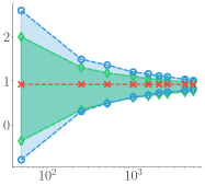
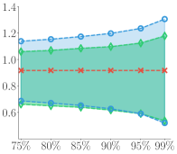
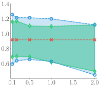
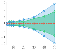
(a) Number of transitions	(b) $1-\delta$	(c) Temperature	(d) Number of features
Rewards
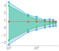
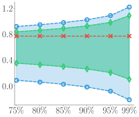
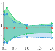
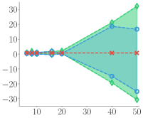
(e) Number of transitions	(f) $1-\delta$	(g) Temperature	(h) Number of features

Figure 1: Results on Inverted-Pendulum (a)-(d) and Puck-Mountain (e)-(h). The plots show the confidence bounds on the average discounted reward as we vary the number of transitions $n$ in (a) & (e), failure probability $\delta$ in (b) & (f), the temperature parameter $\tau$ of the behavior policy in (c) & (g), and the number of features in (d) & (h). The default parameters (when not varied) are: discounted factor $\gamma=0.95$; horizon length $T=50$ for Inverted-Pendulum and $T=100$ for Puck-Mountain; number of episodes $20$; failure probability $\delta=0.10$; temperature of the behavior policy $\tau=1$; and the feature dimension 10.

4.4 Post-hoc Correction of Existing Estimators

In addition to providing confidence bounds around the existing estimator $\widehat{Q}$, we may want to further correct $\widehat{Q}$ when $\widehat{Q}$ is identified to admit large error. The post-hoc correction should ensure the corrected estimation falls into the confidence bounds provided earlier, while keeping the information in $\widehat{Q}$ as much as possible.

Our idea is to correct $\widehat{Q}$ by adding a debiasing term $Q_{\rm{debias}}$, such that $\widehat{L}_{K}^{V}(\widehat{Q}+Q_{\rm{debias}})\leq\lambda_{K}$, while keeping $Q_{\rm{debias}}$ as small as possible. This is framed into

$$\min_{Q_{\rm{debias}}\in\mathcal{F}}\left\{\left\|Q_{\rm{debias}}\right\|_{\mathcal{H}_{K_{0}}}^{2}~{}~{}\text{s.t.}~{}~{}\widehat{L}_{K}(Q+Q_{\rm{debias}})\leq\lambda_{K}\right\}.$$

We should distinguish $Q_{\rm{debias}}$ with the $Q_{\rm{res}}$ in Section 4.3, and $Q_{\rm{res}}$ can not be used for the debiasing purpose because it is designed to give an extreme estimation (for providing the bound), rather than a minimum correction.

In the case of random features approximation, the optimization reduces to

$$\theta^{\star}=\operatorname*{arg\,min}_{\theta}\Big{\{}\|\theta\|_{2}^{2},$$

$$\quad\quad\quad~{}~{}~{}\text{s.t.}~{}~{}~{}\left(Z\theta-\zeta\right)^{\top}M\left(Z\theta-\zeta\right)\leq\lambda_{K}\Big{\}}\,,$$ (18)

and $Q_{\rm{debias}}(x)={\theta^{\star}}^{\top}\Phi(x)$. If the existing estimator $\widehat{Q}$ already satisfies $\widehat{L}_{K}^{V}(\widehat{Q})\leq\lambda_{K}$, this provides a zero correction (i.e., $\theta^{\star}={0}$), since the estimator is already sufficiently accurate. This procedure is summarized in Algorithm 2.

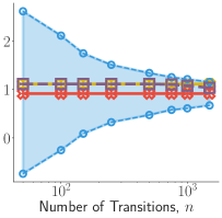
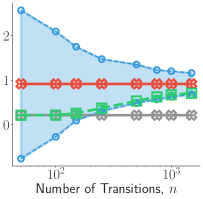
Rewards	Rewards	Norm
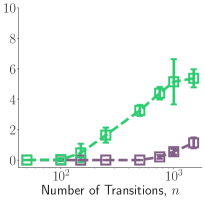
(a) Diagnosis $\widehat{Q}_{1}$ with different $n$	(b) Diagnosis for $\widehat{Q}_{2}$ with different $n$	(c) Norm of $Q_{\rm{debias}}$
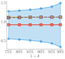
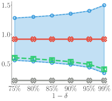
Rewards	Rewards	Norm
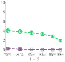
(d) Diagnosis for $\widehat{Q}_{1}$ with different $\delta$	(e) Diagnosis for $\widehat{Q}_{2}$ with different $\delta$	(f) Norm of $Q_{\rm{debias}}$

Figure 2: Post-hoc diagnosis on Inverted-Pendulum. In figure (a)-(c), we vary the number of transitions with fixed $\delta=0.10$. In figure (d)-(f), we fixed number of transitions $n=500$ and vary the failure probability $\delta$. The default parameters are: discounted factor $\gamma=0.95$, the horizon length $T=50$, number of transitions $n=500$, failure probability $\delta=0.10$, temperature of the behavior policy $\tau=1$, and the feature dimension 10.

5 Experiments

We evaluate the proposed algorithms in Section 4 on two continuous control tasks: Inverted-Pendulum and Puck-Mountain. Details of the tasks are in Appendix D.

For all of our experiments, we use a Gaussian RBF kernel $K(x_{i},x_{j})=\exp(-||x_{i}-x_{j}||^{2}_{2}/h^{2})$ for evaluating the kernel Bellman statistics, with a bandwidth selected from a separate batch of training data, and $V$-statistics to calculate Equation (5) given a set of empirical data.

To construct the behavior and target policies, we first train an optimal Q-function using deep Q-learning, and use its softmax functions as policies, and set the temperature to be higher for the behavior policies to encourage exploration. Note that our algorithms do not require to know the behavior policies since they are behavior-agnostic. A description for how to construct policies is in Appendix D.

5.1 Confidence Bounds for Off-Policy Evaluation

We test Algorithm 1 on the two continuous control tasks, Inverted-Pendulum (Figure 1(a)-(d)) and Puck-Mountain (Figure 1(e)-(h)). We solve the convex optimization in Algorithm 1 using CVXPY (Diamond & Boyd, 2016; Agrawal et al., 2018), which gives us the upper and lower bound $\widehat{\eta}^{+}$ and $\widehat{\eta}^{-}$. The results are reported w.r.t. the average discounted reward defined by ${\eta^{\pi}}/{(1-\gamma)}$. The results are averaged over 50 random trials.

We use two types of feature maps $\Phi(\cdot)$ to parameterize the state-action value function $Q(x):=\theta^{\top}\Phi(x)$:

1) Random Fourier features: $\Phi(x):=[\cos(\mu_{i}^{\top}x+b_{i})]_{i=1}^{m}$, where $\mu_{i}\sim\mathcal{N}(0,\frac{1}{h_{0}^{2}}\rm{I})$, $b_{i}\sim\text{Uniform}[0,2\pi]$, and $h_{0}$ is a bandwidth parameter.

2) Neural features. We use a small neural network to parameterize $Q$ function, and learn the $Q$ function by minimizing the kernel loss on the training dataset, and set $\Phi(\cdot)$ by selecting a set of neural features (the neural feature map before the last linear layer) on the validation set.

Figure 1(a)-(d) demonstrate the evaluation results on Inverted-Pendulum. From Figure 1(a) & (b) we can see that, as we increase the number of transitions, or increase the failure probability $\delta$, the confidence bounds become tighter since $\lambda_{K}$ becomes smaller. However, it still covers the ground truth $\eta^{\pi}$, which indicates that our method gives a reasonable confidence interval for off-policy estimation.

In Figure 1(c), we investigate the performance of our method when we vary a temperature parameter of the behavior policy that controls the concentration of the probability mass. The confidence bounds do not change significantly with different temperature of behavior policies. In Figure 1(d), we study the performance of our algorithms with different number of features (including both random Fourier and neural features), which shows that we can get a tight confidence interval when the number of features is small. This is because when decreasing the number of features, the Q function is constrained in a lower dimensional function space and hence gives a tighter confidence interval. However, decreasing the number of features also increases the risk of model misspecification. We also test our method on Puck-Mountain, and report the results in Figure 1 (e)-(h), which show similar results as we observe in Inverted-Pendulum.

5.2 Post-hoc Diagnosis for Existing Estimators

We implement Algorithm 2 to provide post-hoc diagnosis for existing $Q$ estimators, and test it on Inverted-Pendulum (Figure 2) and Puck-Mountain (Figure 3 in the Appendix D). Figure 2 (a)-(f) show the diagnosis results for two different state-action value function estimators ($\widehat{Q}_{1}$ and $\widehat{Q}_{2}$) on Inverted-Pendulum, which we learn with kernel Bellmen statistics using different number of optimization steps. Here $\widehat{Q}_{1}$ is a relatively accurate estimator while the estimation of $\widehat{Q}_{2}$ has larger bias.

Figure 2 (a)-(c) show that as we increase the number of transitions, the norm of the debias term $Q_{\rm{debias}}$ keeps zero when $\widehat{Q}_{1}$ and $\widehat{Q}_{2}$ are inside the confidence interval. Meanwhile, when $\widehat{Q}_{1}$ and $\widehat{Q}_{2}$ can not provide an accurate estimation (falling outside of the confidence interval), our algorithm gives a good post-hoc correction to ensure the corrected estimation are inside the confidence interval. As we can see, such post-hoc diagnosis provides both confidence bounds and correction for existing estimators, which can be useful in real-world applications.

Figure 2 (d)-(f) demonstrate the performance of our algorithms when we change the failure probability $\delta$. Again, the empirical results shows that our algorithms can provide meaningful post-hoc diagnosis.

We also test our method on Puck-Mountain, following the same procedure as on Inverted-Pendulum, which shows similar results as we find in Inverted-Pendulum.

6 Conclusion

In this paper, we develop a new variational framework for constructing confidence bounds for off-policy evaluation and extend it to perform post-hoc diagnosis on existing estimators. In future work, we will leverage our framework to develop safe and efficient policy optimization and exploration algorithms based on the kernel Bellman statistics.

Appendix

Appendix A Proof Concentration Bounds

The proof of concentrations bounds of U/V-statistics are standard topics in probability and statistics. We provide proof here for completeness. In addition, we show that the concentration bounds still hold in non-i.i.d. cases when $Q=Q^{\pi}$ due to a special martingale structure from Bellman equation.

A.1 Proof of Concentration Bound for U-statistics

Assume $X$ is a random variable supported on $\mathcal{X}$. Given some bounded bivariate function $h:\mathcal{X}^{2}\to[a,b]$, the U-statistics of $h$ is defined as:

$$U=\frac{1}{n(n-1)}\sum_{1\leq i\neq j\leq n}h(X_{i},X_{j})\,,$$

where $X_{1},X_{2},\cdots,X_{n}\sim X$ are i.i.d. random variables. It’s well known that U-statistics is an unbiased estimation for $\mathbb{E}_{Y,Z\sim X}[h(Y,Z)]$, and we include the concentration property of U-statistics for completeness.

For simplicity, we assume $n=2k,k\in\mathbb{Z}$ when we discuss the concentration of U-statistics with Hoeffding’s inequality.

Theorem A.1 (Hoeffding’s Inequality for U-statistics).

$$\mathbb{P}\left[\left|U-\mathbb{E}[h]\right|\geq(b-a)\sqrt{\frac{\log\frac{2}{\delta}}{2k}}~{}\right]\leq\delta\,.$$

Proof.

The proof is originated from Hoeffding (1963), and we restate the original proof here for the completeness.

We first introduce the following notation:

$$V(X_{1},X_{2},\cdots,X_{n})=\frac{1}{k}\sum_{i\in[k]}h(X_{2i-1},X_{2i})\,.$$ (19)

It’s easy to see that $\mathbb{E}[V]=\mathbb{E}[h]$, and

$$U=\frac{1}{n!}\sum_{\sigma\in S_{n}}V(X_{\sigma_{1}},X_{\sigma_{2}},\cdots,X_{\sigma_{n}})\,,$$

where $S_{n}$ is the symmetric group of degree $n$ (i.e. we take the summation over all of the permutation of set $[n]$).

With Chernoff’s bound, we can know

$$\mathbb{P}\left[U\geq\delta\right]\leq\exp(-\lambda\delta)\mathbb{E}[\exp(\lambda U)],\quad\forall\lambda>0\,.$$

So we focus on the term $\mathbb{E}\left[\exp(\lambda U)\right]$. With Jensen’s inequality, we have:

$$\mathbb{E}[\exp(\lambda U)]=\mathbb{E}\left[\exp\left(\frac{\lambda}{n!}\sum_{\sigma\in S_{n}}V\left(X_{\sigma_{1}},X_{\sigma_{2}},\cdots,X_{\sigma_{n}}\right)\right)\right]\leq\frac{1}{n!}\sum_{\sigma\in S_{n}}\mathbb{E}\left[\exp(\lambda V(X_{\sigma_{1}},X_{\sigma_{2}},\cdots,X_{\sigma_{n}}))\right].$$

Thus,

$$\mathbb{P}[U-\mathbb{E}[h]\geq\delta]\leq\frac{1}{n!}\sum_{\sigma\in S_{n}}\mathbb{E}\left[\exp\left(\lambda V(X_{\sigma_{1}},X_{\sigma_{2}},\cdots,X_{\sigma_{n}})-\lambda\mathbb{E}[h]-\lambda\delta\right)\right].$$

Notice that, $V$ is sub-Gaussian with variance proxy $\sigma^{2}=\frac{(b-a)^{2}}{4k}$. Thus, with the property of sub-Gaussian random variable,

$$\mathbb{E}\left[\exp\left(\lambda V-\lambda\mathbb{E}[h]-\lambda\delta\right)\right]\leq\exp\left(\frac{\lambda^{2}(b-a)^{2}}{8k}-\lambda\delta\right),\quad\forall\lambda>0.$$

When $\lambda=\frac{4k\delta}{(b-a)^{2}}$, $\exp(\frac{\lambda^{2}(b-a)^{2}}{8k}-\lambda\delta)$ achieves the minimum $\exp(-\frac{2k\delta^{2}}{(b-a)^{2}})$. Thus,

$$\mathbb{P}\left[U-\mathbb{E}[h]\geq\delta\right]\leq\frac{1}{n!}\sum_{\sigma\in S_{n}}\exp\left(-\frac{2k\delta^{2}}{(b-a)^{2}}\right)=\exp\left(-\frac{2k\delta^{2}}{(b-a)^{2}}\right).$$

Moreover, with the symmetry of $U$, we have that:

$$\mathbb{P}[|U-\mathbb{E}[h]|\geq\delta]\leq 2\exp\left(-\frac{2k\delta^{2}}{(b-a)^{2}}\right),$$

which concludes the proof. ∎

A.2 Concentration Bounds for V-statistics

We have the following equation for U-statistics and V-statistics

$$\widehat{L}_{K}^{V}(Q)=\frac{n-1}{n}\widehat{L}_{K}^{U}(Q)+\sum_{i\in[n]}\ell_{\pi,Q}(\tau_{i},\tau_{i})\,,$$

so we can upper bound $|\widehat{L}_{K}^{V}(Q)-L_{K}(Q)|$ via

$$|\widehat{L}_{K}^{V}(Q)-L_{K}(Q)|\leq\frac{n-1}{n}|\widehat{L}_{K}^{U}(Q)-L_{K}(Q)|+\left|\frac{1}{n^{2}}\sum_{i\in[n]}\ell_{\pi,Q}(\tau_{i},\tau_{i})-\frac{1}{n}L_{K}(Q)\right|\,.$$

Thus, with the concentration bounds of $\widehat{L}_{K}^{U}(Q)$, and the fact that $|\ell_{\pi,Q}(\tau_{i},\tau_{i})|\leq\ell_{\max}$, and $|L_{K}(Q)|\leq\ell_{\max}$, we have the desired result.

A.3 Concentration Bounds for Non I.I.D. Samples

In practice, the dataset $\mathcal{D}=\{x_{i},r_{i},s_{i}^{\prime}\}_{1\leq i\leq n}$ can be obtained with a non i.i.d fasion (such as we collect trajectories in the MDP follow by a policy $\pi$), which violates the assumption that samples from $\mathcal{D}$ are drawn independently. There are concentration bounds for U-statistics with weakly dependent data. For example, Han (2018) considers the concentration of U-statistics when the data are generated from a Markov Chain under mixing conditions. Here we show that, in the case when $Q=Q^{\pi}$, the concentration inequality holds without requiring the i.i.d. or any mixing condition, thanks to a martingale structure from the Bellman equation.

Proposition A.1.

Assume the transitions are sampled from the MDP, i.e. $s^{\prime}\sim\mathcal{P}(\cdot|x)$, $\bar{s}^{\prime}\sim\mathcal{P}(\cdot|\bar{x})$, then for any joint measure $\nu$ of $(x,\bar{x})$, we have the following property for $Q^{\pi}$:

$$\mathbb{E}_{(x,\bar{x})\sim\nu,s^{\prime}\sim\mathcal{P}(\cdot|x),\bar{s}^{\prime}\sim\mathcal{P}(\cdot|\bar{x})}[K(x,\bar{x})\cdot\widehat{\mathcal{R}}_{\pi}Q^{\pi}(x)\cdot\widehat{\mathcal{R}}_{\pi}Q^{\pi}(\bar{x})]=0\,,$$

For i.i.d. case, $\nu=\mu\times\mu$.

Proof.

By the definition of Bellman error for $Q$-function, we have that

$$\mathbb{E}_{s^{\prime}\sim\mathcal{P}(\cdot|x)}\left[\widehat{\mathcal{R}}_{\pi}Q^{\pi}(x)\right]=\mathbb{E}_{x^{\prime}\sim\mathcal{P}(\cdot|x)\times\pi(\cdot|s^{\prime})}\left[\widehat{\mathcal{R}}_{\pi}Q^{\pi}(x)\right]=0\,.$$

As we can first take expectation w.r.t $s^{\prime}$ and $\bar{s}^{\prime}$, we can conclude the proof. ∎

Theorem A.2 (Concentration Bounds with Non I.I.D. Samples).

Consider a set of random transition pairs $\{\tau_{i}\}_{i=1}^{n}$ with $\tau_{i}=(s_{i},a_{i},r_{i},s_{i}^{\prime})$. Assume the state-action pairs $(s_{i},a_{i})_{i=1}^{n}$ are drawn from an arbitrary joint distribution, and given $(s_{i},a_{i})_{i=1}^{n}$, the local rewards and next states $(r_{i},s_{i}^{\prime})_{i=1}^{n}$ is drawn independently from $r_{i}=r(s_{i},a_{i})$ and $s_{i}^{\prime}\sim\mathcal{P}(\cdot~{}|~{}s_{i},a_{i})$.

Then $\forall\delta\in(0,1)$, we have the following concentration inequality for $Q^{\pi}$:

$$\mathbb{P}\left[~{}~{}\left|\widehat{L}_{K}^{U}(Q^{\pi})\right|\geq 2\ell_{\max}\sqrt{\frac{\log\frac{2}{\delta}}{n}}~{}~{}\right]\leq\delta\,.$$

where $\ell_{\max}$ is given via Lemma 3.1.

Proof.

First, $\forall~{}(x,s^{\prime}),(\bar{x},\bar{s}^{\prime})$ pair, where $s^{\prime}\sim\mathcal{P}(\cdot|x)$, $\bar{s}^{\prime}\sim\mathcal{P}(\cdot|\bar{x})$, from the proof of Proposition A.1, we can know

$$\mathbb{E}_{s^{\prime}\sim\mathcal{P}(\cdot|x),\bar{s}^{\prime}\sim\mathcal{P}(\cdot|\bar{x})}[K(x,\bar{x})\cdot\widehat{\mathcal{R}}_{\pi}Q^{\pi}(x)\cdot\widehat{\mathcal{R}}_{\pi}Q^{\pi}(\bar{x})]=0\,.$$

Then we revisit the definition of $V$ in Equation (19):

$$V(X_{1},X_{2},\cdots,X_{n})=\frac{1}{k}\sum_{i\in[k]}h(X_{2i-1},X_{2i})\,.$$

For kernel Bellman statistic, $X_{i}=(x_{i},s_{i}^{\prime})$, where $s_{i}^{\prime}\sim\mathcal{P}(\cdot|x_{i})$, and $h(X_{i},X_{j})=K(x_{i},x_{j})\cdot\widehat{\mathcal{R}}_{\pi}Q^{\pi}(x_{i})\cdot\widehat{\mathcal{R}}_{\pi}Q^{\pi}(x_{j})$. With Proposition A.1, we have that

$$\mathbb{E}_{x_{2i-1},x_{2i},s_{2i-1}^{\prime}\sim\mathcal{P}(\cdot|x_{2i-1}),s_{2i}^{\prime}\sim\mathcal{P}(\cdot|x_{2i})}\left[K(x_{2i-1},x_{2i})\cdot\widehat{\mathcal{R}}_{\pi}Q^{\pi}(x_{2i-1})\cdot\widehat{\mathcal{R}}_{\pi}Q^{\pi}(x_{2i})~{}\big{|}~{}x_{1},\cdots,x_{2i-2}\right]=0\,,$$

as the expectation doesn’t depend on how we get $x_{2i-1}$ and $x_{2i}$, but $s_{2i-1}^{\prime}\sim\mathcal{P}(\cdot|x_{2i-1})$, $s_{2i}^{\prime}\sim\mathcal{P}(\cdot|x_{2i})$. So we can view $V$ as a summation of bounded martingale differences.

By using the Azuma’s inequality for the martingale differences, we can show:

$$\mathbb{E}\left[\exp(\lambda V)\right]\leq\exp\left(\frac{\lambda^{2}(b-a)^{2}}{8k}\right)\,.$$

So the Hoeffding-type bound still holds, following the derivation of Appendix A.1. ∎

Remark We have proved that if the environment is Markovian, we still have the desired Hoeffding-type concentration bound for $Q^{\pi}$, and our algorithms are still valid given non i.i.d. samples. However, in practice, we still need the data collecting process to be ergodic (which is a general assumption (Puterman, 1994)), as we want to estimate $Q^{\pi}$ over all of the $\mathcal{S}\times\mathcal{A}$.

Remark If we want to consider any $Q$ function other than $Q^{\pi}$, the non i.i.d $x$ will lead to an additional bias term, which can be difficult to estimate empirically . We leave this as a future work.

Remark Notice that, here we only use the universal upper bound of $\ell_{\pi,Q}(\tau_{i},\tau_{i})$, so the bound for $Q^{\pi}$ is still valid for non i.i.d dataset $\mathcal{D}=\{x_{i},r_{i},s_{i}\}_{1\leq i\leq n}$ if we use Hoeffding-type bound for U-statistics.

Appendix B Proof of Lemmas

See 3.1

Proof.

Recall the definition of $Q^{\pi}$, we have

$$Q^{\pi}(x)=\mathbb{E}_{\pi}\left[\sum_{t=0}^{\infty}\gamma^{t}|s_{0}=s,a_{0}=a\right]\leq\left(\sum_{t=0}^{\infty}{\gamma}^{t}\right)r_{\max}=\frac{r_{\max}}{1-\gamma},~{}~{}\forall~{}x\,.$$

Recall the definition of $\ell_{\pi,Q^{\pi}}(\tau,\bar{\tau})$ in (6), we have

$$|\ell_{\pi,Q^{\pi}}(\tau,\bar{\tau})| =\left|\left(Q(x)-r(x)-\gamma Q(x^{\prime})\right)K(x,\bar{x})\left(Q(\bar{x})-r(\bar{x})-\gamma Q(\bar{x}^{\prime})\right)\right|$$

$$\leq\sup_{x,\bar{x}}|K(x,\bar{x})|\cdot\sup_{\tau}\left(Q(x)-r(x)-\gamma Q(x^{\prime})\right)^{2}$$

$$\leq K_{\max}\cdot\left(\frac{r_{\max}}{1-\gamma}+r_{\max}+\gamma\cdot\frac{r_{\max}}{1-\gamma}\right)^{2}$$

$$=\frac{4K_{\max}r^{2}_{\max}}{(1-\gamma)^{2}}\,.$$

∎

Appendix C Accountable Off-Policy Evaluation for Average Reward $(\gamma=1)$

In this section, we generalize our methods to the average reward setting where $\gamma=1$. Denote by $M=\langle\mathcal{S},\mathcal{A},\mathcal{P},r,\gamma\rangle$ a Markov decision process (MDP), where $\mathcal{S}$ is the state space; $\mathcal{A}$ is the action space; $\mathcal{P}(s^{\prime}|s,a)$ is the transition probability; $r(s,a)$ is the average immediate reward; $\gamma=1$ (undiscounted case). The expected reward of a given policy $\pi$ is

$$\eta^{\pi}=\lim_{T\to\infty}\frac{1}{T+1}\mathbb{E}_{\pi}\left[\sum_{t=0}^{T}r_{t}\right]\,.$$

In the discounted case ($0<\gamma<1$), the value function $Q^{\pi}(s,a)$ is the expected total discounted reward when the initial state $s_{0}$ is fixed to be $s$, and $a\sim\pi(\cdot|s)$: $Q^{\pi}(s,a)=\mathbb{E}_{\tau\sim\pi_{\pi}}[\sum_{t=0}^{\infty}\gamma^{t}r_{t}|s_{0}=s,a_{0}=a]$. If the Markov process is ergodic (Puterman, 1994), the expected average reward does not depend on the initial states. In the average case, however, $Q^{\pi}(s,a)$ measures the average adjusted sum of reward:

$$Q^{\pi}(s,a):=\lim_{T\to\infty}\mathbb{E}_{\pi}\left[\sum_{t=0}^{T}(r_{t}-\eta^{\pi})~{}\big{|}~{}s_{0}=s,a_{0}=a\right]\,,$$

which is referred to as the adjusted (state-action) value function.

Under this definition, $(Q^{\pi},\eta^{\pi})$ is the unique fixed-point solution to the following Bellman equation:

$$Q(s,a)=\mathbb{E}_{s^{\prime}\sim\mathcal{P}(\cdot|s,a),a^{\prime}\sim\pi(\cdot|s^{\prime})}[r(s,a)+Q(s^{\prime},a^{\prime})-\eta]\,.$$ (20)

To simplify notation, we still assume $x=(s,a)$, $\bar{x}=(\bar{s},\bar{a})$, and $x^{\prime}:=(s^{\prime},a^{\prime})$ with $s^{\prime}\sim\mathcal{P}(\cdot|s,a),a^{\prime}\sim\pi(\cdot|s^{\prime})$. Define the Bellman residual operator as

$$\mathcal{R}_{\pi}Q(x)=\mathbb{E}_{s^{\prime}\sim\mathcal{P}(\cdot|s,a),a^{\prime}\sim\pi(\cdot|s^{\prime})}\left[r(x)+Q(x^{\prime})-\eta\right]-Q(x)\,,$$

where $Q$ is an estimation of adjusted value function, and $\eta$ is an estimation of the expected reward. Note that $\mathcal{R}_{\pi}Q(x)$ depends on both $Q$ and $\eta$, even though it is not indicated explicitly on notation. Given a $(Q,\eta)$ pair, the kernel loss for $\gamma=1$ can be defined as

$$L_{K}(Q,\eta):=\mathbb{E}_{x,\bar{x}\sim\mu}[\mathcal{R}_{\pi}Q(x)\cdot K(x,\bar{x})\cdot\mathcal{R}_{\pi}Q(\bar{x})]\,.$$

Given a set of observed transition pairs $\mathcal{D}=\{\tau_{i}\}_{i=1}^{n}$, and we can estimate $L_{K}(Q,\eta)$ with the following V-statistics:

$$\widehat{L}_{K}^{V}(Q,\eta)= \frac{1}{n^{2}}\sum_{i,j=1}^{n}\ell_{\pi,Q}(\tau_{i},\tau_{j})\,,$$

where

$$\ell_{\pi,Q}(\tau_{i},\tau_{j})=\widehat{\mathcal{R}}_{\pi}Q(x_{i})K(x_{i},x_{j})\widehat{\mathcal{R}}_{\pi}Q(x_{j})\,,$$

and

$$\widehat{\mathcal{R}}_{\pi}Q(x_{i})=r(x_{i})+\mathbb{E}_{a_{i}^{\prime}\sim\pi(\cdot|s_{i}^{\prime})}\left[Q(x_{i}^{\prime})\right]-\eta-Q(x_{i}).$$

Similarly, we can estimate $L_{K}(Q,\eta)$ via U-statistics:

$$\widehat{L}_{K}^{U}(Q,\eta)=\frac{1}{n(n-1)}\sum_{1\leq i\neq j\leq n}\ell_{\pi,Q}(\tau_{i},\tau_{j})\,.$$

C.1 Concentration Bounds for U-/V-statistics

Here we derive the concentration bounds of the U-/V-statistics for the average reward case, under the mild assumption that the reward $r(x)$ and $Q(x)$ are bounded.

Lemma C.1.

Assume the reward function, the adjusted (state-action) value function and the kernel function are uniformly bounded, i.e. $\sup_{s\in\mathcal{S},a\in\mathcal{A}}|r(x)|\leq r_{\max}$, $\sup_{s\in\mathcal{S},a\in\mathcal{A}}|Q^{\pi}(x)|\leq Q_{\max}$, $\sup_{x,\bar{x}}|K(x,\ \bar{x})|\leq K_{\max}$. Then we have

$$\sup_{\tau,\bar{\tau}}|\ell_{\pi,Q^{\pi}}(\tau,\bar{\tau})|\leq\ell_{\max}:=4K_{\max}(Q_{\max}+r_{\max})^{2}\,.$$

Proof.

By definition, we have

$$\sup_{\tau,\bar{\tau}}|\ell_{\pi,Q^{\pi}}(\tau,\bar{\tau})| \leq|r_{\max}+Q_{\max}-(-r_{\max})-(-Q_{\max})|^{2}\cdot|K(x,\bar{x})|$$

$$\leq 4K_{\max}(Q_{\max}+r_{\max})^{2}.$$

∎

With a similar derivation in Appendix A, we can have the same Hoeffding-type bounds for U/V-statistics as that of the discounted case, which can be utilized to construct the confidence interval for $\eta^{\pi}$.

C.2 Confidence Bounds for Average Reward

As our final target is to build the confidence interval for the average reward, we follow a similar idea as the discounted case to obtain a high probability upper bound of the expected reward $\eta^{\pi}$ by solving the following optimization problem:

$$\max_{|\eta|\leq r_{\max},Q\in\mathcal{F},}\left\{~{}~{}\eta\quad\text{s.t.}\quad\widehat{L}_{K}^{V}(Q,\eta)\leq\lambda_{K}\right\}\,,$$

where $\eta$ is a scalar variable and $Q\in\mathcal{F}$ is the adjusted value function, which we want to jointly optimize.

C.3 Optimization in RKHS

Similar to the discounted case, we can use random feature approximation to speed up the optimization. In this case, the optimization reduces to

$$\widehat{\eta}^{+}=\max_{|\eta|\leq r_{\max},\theta}\left\{\eta,~{}~{}~{}~{}\text{s.t.}~{}~{}~{}\left(Z\theta+\eta-v\right)^{\top}M\left(Z\theta+\eta-v\right)\leq\lambda_{K}\right\}\,.$$

where the constants are the same as these defined in Section 4.2, except that $Z=X-X^{\prime}$.

Appendix D Experiments

In this section, we provide the details of the experiments, and some additional experiments for validating the effectiveness of our method.

D.1 Experimental Details

Evaluation Environments

We evaluate the proposed algorithms in Section 4 on two continuous control tasks: Inverted-Pendulum and Puck-Mountain.

Inverted-Pendulum is a pendulum that has its center of mass above its pivot point. It has a continuous state space on $\mathbb{R}^{4}$. We discrete the action space to be $\{-1,-0.3,-0.2,0,0.2,0.3,1\}$. The pendulum is unstable and would fall over without careful balancing. We train a near optimal policy that can make the pendulum balance for a long horizon using deep Q learnings, and use its softmax function as policies. We set the temperature to be higher for the behavior policies to encourage exploration. We use the implementation from OpenAI Gym (Brockman et al., 2016) and change the dynamic by adding some additional zero mean Gaussian noise to the transition dynamic.

Puck-Mountain is an environment similar to Mountain-Car, except that the goal of the task is to push the puck as high as possible in a local valley whose initial position is at the bottom of the valley. If the ball reaches the top sides of the valley, it will hit a roof and change the speed to its opposite direction with half of its original speeds. The reward was determined by the current velocity and height of the puck. The environment has a $\mathbb{R}^{2}$ state space, and a discrete action space with 3 possible actions (pushing left, no pushing, and pushing right). We also add zero mean Gaussian perturbations to the transition dynamic to make it stochastic.

Policy Construction

We use the open source implementation of deep Q-learning to train a $32\times 32$ MLP parameterized Q-function to converge. We then use the softmax policy of the learned Q-function with different temperatures as policies. We set a default temperature $\tau=0.1$ (to make it more deterministic) for the target policy $\pi$. For behavior policies, we set the temperature $\tau=1$ as default. We also study the performance of our method under behavior policies with different temperatures to demonstrate the effectiveness of our method under behavior agnostic settings.

Hyperparameters Selection and Neural Feature Learning

For all of our experiments, we use Gaussian RBF kernel $K(x,\bar{x})=\exp\left(-||x-\bar{x}||^{2}_{2}/h^{2}\right)$ in the kernel Bellman kernel (e.g., for Equation (5)). We evaluate the kernel Bellman loss on a separate batch of training data, and find that we can set the bandwidth to $h=0.5$, which will give a good solution.

When we parameterize $Q$ function $Q(x):=\theta^{\top}\Phi(x)$with random Fourier features: $\Phi(x):=[\cos(\mu_{i}^{\top}x+b_{i})]_{i=1}^{m}$, where $\mu_{i}\sim\mathcal{N}(0,\frac{1}{h_{0}^{2}}\rm{I})$, $b_{i}\sim\text{Uniform}([0,2\pi])$, and $h_{0}$ is a bandwidth parameter. We select the bandwidth $h_{0}$ from a candidate set $\Pi=\{h_{1},h_{2},\ldots,h_{k}\}$ by finding the smallest lower bound and largest upper bound on a separate validation data. Specifically, for each $h_{i}\in\Pi$, we follow the procedure of Algorithm 1 to calculate an upper and lower bounds for $\eta^{\pi}$, and select the lowest lower bound and the largest upper bound as our final bounds. Doing this ensures that our bounds are pessimistic and safe. In our empirical experiments we set $\Pi=\{0.2,0.5,0.6,0.8,1.0\}$.

Following the similar procedure, we also select a set of neural features (the neural feature map before the last linear layer) on the validation set, which have relatively lower kernel loss when we optimize the neural network. Similarly, we select two different neural features for each environment and use the pessimisitc upper and lower bounds for all of our experiments.

Constructing Existing Estimators in Post-hoc Diagnosis

Since we only need to demonstrate the effectiveness of our proposed post-hoc diagnosis process, we simply parameterize Q as a linear function of a small set of random Fourier features ($Q(\cdot)=\theta^{\top}\Phi(\cdot)$), and estimate $\theta$ by minimizing the kernel Bellman loss by running gradient descent for different numbers of iterations. For the experiments in Inverted-Pendulum (Figure 2), $\widehat{Q}_{1}$ (resp. $\widehat{Q}_{2}$) are obtained when we run a large (resp. small) number of iterations in training, so that $\widehat{Q}_{1}$ is relatively accurate while $\widehat{Q}_{2}$ is not. For Puck-Mountain in Figure 3, the error of both $\widehat{Q}_{1}$ and $\widehat{Q}_{2}$ are relatively large.

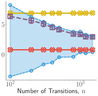
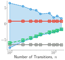
Rewards	Rewards	Norm
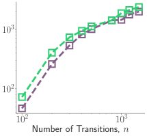
(a) Diagnosis $\widehat{Q}_{1}$ with different $n$	(b) Diagnosis for $\widehat{Q}_{2}$ with different $n$	(c) Norm of $Q_{\rm{debias}}$
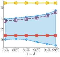
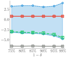
Rewards	Rewards	Norm
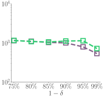
(d) Diagnosis for $\widehat{Q}_{1}$ with different $\delta$	(e) Diagnosis for $\widehat{Q}_{2}$ with different $\delta$	(f) Norm of $Q_{\rm{debias}}$

Figure 3: Post-hoc diagnosis on Puck-Mountain. We set the discounted factor $\gamma=0.95$, the horizon length $T=100$, number of transitions $n=500$, failure probability $\delta=0.10$, temperature of the behavior policy $\tau=1$, and the feature dimension 10 as default. The rest of the parameters are the same as that in Section 5.

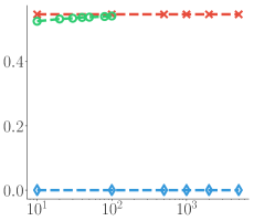
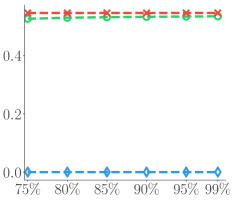
Normalized Reward	Normalized Rewards	Normalized Rewards
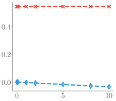
(a) Number of Episodes, $N$	(b) $1-\delta$	(c) Threshold value $c$

Figure 4: IS-based confidence lower bounds Thomas et al. (2015a) on Inverted-Pendulum following the same setting as that in Section 5. We use the results of random Fourier feature in Figure 1 as our lower bound. For Thomas et al. (2015a), we set the threshold value to be $c=10^{-5}$ in (a) & (b), and the number of episodes $N=2000$ in (b) & (c). For our method, we only use $n=50\times 20$ number of transition pairs in (b). We report the normalized reward based on the procedure in Thomas et al. (2015a) (${\rho_{\rm{normalize}}}=(\sum_{t=1}^{T}\gamma^{t-1}r_{t}-R_{\min})/(R_{\max}-R_{\min})$).

D.2 Additional Experiments

Post-hoc Diagnosis Experiments on Puck-Mountain

Figure 3 (a)-(f) show the diagnosis results for two estimations of Q-function ($\widehat{Q}_{1}$ and $\widehat{Q}_{2}$) on Puck-Mountain. Here both $\widehat{Q}_{1}$ and $\widehat{Q}_{2}$ have relatively large bias, but $\widehat{Q}_{1}$ tends to overestimate $\eta^{\pi}$ (see Figure 3(a)), while $\widehat{Q}_{2}$ tends to underestimate $\eta^{\pi}$ (see Figure 3).

Figure 3(a)-(c) show that as we increase the number of transitions, the norm of the debiasing term $Q_{\rm{debias}}$ becomes larger. This is because when we have more data, we have a relatively tight confidence bound and we need a more complex debias function to provide good post-hoc correction. Figure 3 (d)-(f) demonstrate the performance of our algorithms when we change the failure probability $\delta$.

Comparison with Thomas et al. (2015a)

As a comparison, we implement the method from Thomas et al. (2015a), which uses concentration inequality to construct confidence bounds on an importance sampling (IS) based estimator. Following Thomas et al. (2015a), we assume the expected reward is normalized as follows

$$\rho^{\pi}_{\rm{normalize}}:=\frac{\mathbb{E}_{\pi}\left[\sum_{t=1}^{T}\gamma^{t-1}r_{t}\right]-R_{\min}}{R_{\max}-R_{\min}}\,,$$ (21)

where $\sum_{t=1}^{T}\gamma^{t-1}r_{t}$ is the discounted return of a trajectory following policy $\pi$, and $R_{\max}$ and $R_{\min}$ are the upper and lower bounds on $\sum_{t=1}^{T}\gamma^{t-1}r_{t}$; see Thomas et al. (2015a) for the choice of $R_{\max}$ and $R_{\min}$.

Given a set of trajectories $\{(s_{t}^{(i)},a_{t}^{(i)},r_{t}^{(i)})_{t=1}^{T}\}_{1\leq i\leq N}$ generated by behavior policy $\pi_{0}$, we have

$$\widehat{\rho}^{\pi}_{\rm IS}:=\frac{1}{N}\sum_{i=1}^{N}X_{i},~{}~{}~{}~{}~{}\text{with}~{}~{}~{}~{}~{}X_{i}=\underbrace{R_{i}}_{\text{return}}\underbrace{\prod_{t=1}^{T}\frac{\pi(a_{t}^{(i)}|s_{t}^{(i)})}{\pi_{0}(a_{t}^{(i)}|s_{t}^{(i)})}}_{\text{importance weight}}\,,$$ (22)

where $R_{i}$ is reward the $i$-th trajectory from the data (normalized as shown in Eq (21)). Theorem 1 in Thomas et al. (2015a) provides a concentration inequality for constructing lower bound of $\rho^{\pi}_{\rm{normalize}}$ based on a truncated importance sampling estimator. Let $\{c_{i}\}_{i=1}^{N}$ be a set of positive real-valued threshold and $\delta\in(0,1)$ and $Y_{i}=\min\{X_{i},c_{i}\}$, we have with probability at least $1-\delta$,

$$\rho^{\pi}_{\rm{normalize}}\geq\underbrace{\left(\sum_{i=1}^{N}\frac{1}{c_{i}}\right)^{-1}\sum_{i=1}^{N}\frac{Y_{i}}{c_{i}}}_{\text{empirical mean}}-\underbrace{\left(\sum_{i=1}^{N}\frac{1}{c_{i}}\right)^{-1}\frac{7N\ln(2/\delta)}{3(N-1)}}_{\text{ term that goes to zero as $1/N$ as $N\to\infty$}}-\underbrace{\left(\sum_{i=1}^{N}\frac{1}{c_{i}}\right)^{-1}\sqrt{\frac{\ln(2/\delta)}{N-1}\sum_{i,j=1}^{N}\left(\frac{Y_{i}}{c_{i}}-\frac{Y_{j}}{c_{j}}\right)^{2}}}_{\text{term that goes to zero as $1/\sqrt{N}$ as $N\to\infty$}}\,.$$ (23)

The RHS provides a lower bound of $\rho^{\pi}_{\rm{normalized}}$ based the empirical trajectories. Following the settings in Thomas et al. (2015a), we set the threshold values to be a constant $c$, that is, $c_{i}=c$ for all $i=1,\ldots,N$.

We evaluate the method on Inverted-Pendulum under the same default settings as our experiments in the paper. Figure 4(a)-(c) show the results of the high confidence lower bound. We can see that the IS lower bounds are almost vacuous (i.e., very close to zero) and it does not help very much when we increase the number of episodes (up to $N=2000$) or the failure probability $\delta$. This is because there is only small overlap between the target policy $\pi$ and behavior policy $\pi_{0}$ in this case and when the horizon length is large ($T=50$), making the IS estimator degenerate. Although we need to point out that to get tighter lower bound with our method, we assume the true $Q^{\pi}$ is in the function space $\mathcal{F}$ that we choose, and also assume the horizon length $T\to\infty$ to make the confidence bound provably hold.

Appendix E Discussion on Reproducing Kernel Hilbert Space

We provide proof of Proposition 4.2 and discussion for Section 4.2.

Proof of Proposition 4.2.

Consider the Lagrangian of the constrained optimization (10), we have:

$$L(Q,\lambda_{1},\lambda_{2})= \mathbb{E}_{x\sim\mu_{0}\times\pi}[Q(x)]-\lambda_{1}(\widehat{L}_{K}(Q)-\lambda_{K})-\lambda_{2}(\|Q\|_{\mathcal{H}}^{2}-\rho)$$

$$= \langle Q,f_{0}\rangle-\frac{\lambda_{1}}{n^{2}}\left(\sum_{i,j}(\langle Q,f_{i}\rangle-r_{i})K(x_{i},x_{j})(\langle Q,f_{j}\rangle-r_{j})\right)-\lambda_{2}(\|Q\|_{\mathcal{H}}^{2})-C,$$

where $\lambda_{1},\lambda_{2}$ are Lagrangian multipliers with respect to the two constraints, and $C$ is a constant related to $\lambda_{1},\lambda_{2},\lambda_{K}$ and $\rho$. We rewrite $Q$ into

$$Q=\sum_{k=0}^{n}\alpha_{k}f_{k}+Q_{\perp},$$

where $Q_{\perp}$ is in the orthogonal subspace to the linear span of $f_{0},f_{1},...,f_{n}$, that is, $\langle f_{i},Q_{\perp}\rangle=0,~{}\forall i\in[n]$. By decomposin $Q$ into $\sum_{k=0}^{n}\alpha_{k}f_{k}$ and $Q_{\perp}$, we have

$$L(Q,\lambda_{1},\lambda_{2})+C= \langle Q,f_{0}\rangle-\frac{\lambda_{1}}{n^{2}}\left(\sum_{i,j}(\langle Q,f_{i}\rangle-r_{i})K(x_{i},x_{j})(\langle Q,f_{j}\rangle-r_{j})\right)-\lambda_{2}(\|Q\|_{\mathcal{H}}^{2})$$

$$= \langle\sum_{k=0}^{n}\alpha_{k}f_{k}+Q_{\perp},f_{0}\rangle-\frac{\lambda_{1}}{n^{2}}\left(\sum_{i,j=1}^{n}(\langle\sum_{k=0}^{n}\alpha_{k}f_{k}+Q_{\perp},f_{i}\rangle-r_{i})K(x_{i},x_{j})(\langle\sum_{k=0}^{n}\alpha_{k}f_{k}+Q_{\perp},f_{j}\rangle-r_{j})\right)$$

$$-\lambda_{2}(\|\sum_{k=0}^{n}\alpha_{k}f_{k}\|_{\mathcal{H}}^{2}+\|Q_{\perp}\|_{\mathcal{H}}^{2})$$

$$= \langle\sum_{k=0}^{n}\alpha_{k}f_{k},f_{0}\rangle-\frac{\lambda_{1}}{n^{2}}\left(\sum_{i,j=1}^{n}(\langle\sum_{k=0}^{n}\alpha_{k}f_{k},f_{i}\rangle-r_{i})K(x_{i},x_{j})(\langle\sum_{k=0}^{n}\alpha_{k}f_{k},f_{j}\rangle-r_{j})\right)$$

$$-\lambda_{2}(\|\sum_{k=0}^{n}\alpha_{k}f_{k}\|_{\mathcal{H}}^{2}+\|Q_{\perp}\|_{\mathcal{H}}^{2})$$

$$\leq \langle\sum_{k=0}^{n}\alpha_{k}f_{k},f_{0}\rangle-\frac{\lambda_{1}}{n^{2}}\left(\sum_{i,j=1}^{n}(\langle\sum_{k=0}^{n}\alpha_{k}f_{k},f_{i}\rangle-r_{i})K(x_{i},x_{j})(\langle\sum_{k=0}^{n}\alpha_{k}f_{k},f_{j}\rangle-r_{j})\ell\right)$$

$$-\lambda_{2}(\|\sum_{k=0}^{n}\alpha_{k}f_{k}\|_{\mathcal{H}}^{2}):=L(\alpha,\lambda_{1},\lambda_{2}),$$

where the optimum $Q$ will have $Q_{\perp}=0$ and $L(\alpha,\lambda_{1},\lambda_{2})$ is the Lagrangian w.r.t. to coefficient $\alpha$. Collecting the term we can reform the optimization w.r.t. $\alpha$ as

$$\widehat{\eta}^{+}:=\max_{\{\alpha_{i}\}_{0\leq i\leq n}}\Big{\{}[c^{\top}\alpha+\lambda_{\eta}],~{}~{}~{}~{}~{}~{}~{}~{}~{}\text{s.t.}~{}~{}\alpha^{\top}A\alpha+b^{\top}\alpha+d\leq 0,~{}~{}~{}~{}~{}~{}~{}~{}~{}\alpha^{\top}B\alpha\leq\rho.\Big{\}}\,$$

where $B_{ij}=\langle f_{i},f_{j}\rangle_{\mathcal{H}_{K_{0}}},~{}\forall 0\leq i,j\leq n$ is the inner product matrix of $\{f_{i}\}_{0\leq i\leq n}$ under $\mathcal{H}_{K_{0}}$, $c$ as the first column of $B$ and $B_{1}$ be the remaining sub-matrix. Let $M_{ij}=K(x_{i},x_{j})$ be the kernel matrix, $R_{i}=r_{i}$ be the vector of reward from data, then $A=\frac{1}{n^{2}}B_{1}MB_{1}^{\top}$, $b=-\frac{1}{n^{2}}B_{1}MR$ and $d=\frac{1}{n^{2}}R^{\top}MR-\lambda_{K}$. ∎

Random Feature Approximation

Consider the random feature representation of kernel $K_{0}$

$$K_{0}(x,x^{\prime})=\mathbb{E}_{w\sim\mu}[\phi(x,w)\phi(x^{\prime},w)],$$ (24)

where $\mu$ is a distribution of random variable $w$. Every function $f$ in the RKHS $\mathcal{H}_{K_{0}}$ associated with $K_{0}$ can be represented as

$$f(x)=\mathbb{E}_{w\sim\mu}[\phi(x,w)\alpha_{f}(w)],$$

whose RKHS norm equals

$$\|f\|_{\mathcal{H}_{K_{0}}}^{2}=\mathbb{E}_{w\sim\mu}[\alpha_{f}(w)^{2}].$$

To approximate $K_{0}$, we draw an i.i.d. sample $\{w_{i}\}$ from $\mu$ to approximate $K_{0}$ with

$$\widehat{K_{0}}(x,x^{\prime})=\frac{1}{m}\sum_{i=1}^{m}\phi(x,w_{i})\phi(x^{\prime},w_{i}).$$ (25)

Similarly, each $f\in\mathcal{H}_{\widehat{K_{0}}}$ can be represented as

$$f(x)=\frac{1}{m}\sum_{i=1}^{m}\phi(x,w_{i})\alpha_{i}$$

and its corresponding RKHS norm is

$$\|f\|_{\mathcal{H}_{\widehat{K_{0}}}}^{2}=\frac{1}{m}\sum_{i=1}^{m}\alpha_{i}^{2}.$$

Denote by $\theta=\alpha/m$, then we have $f(x)=\theta^{\top}\Phi(x)$ and $\left\|f\right\|^{2}_{\mathcal{H}_{\widehat{K_{0}}}}=m\left\|\theta\right\|_{2}^{2}$, which is the form used in the paper.

The result below shows that when $Q^{\pi}$ is included in $\mathcal{H}_{K_{0}}$ but may not be included in $\mathcal{H}_{\widehat{K}_{0}}$, we can still get a provably upper bound by setting the radius of the optimization domain properly large.

Theorem E.1.

Let $K_{0}$ be a positive definite kernel with random feature expansion in (24) and $\widehat{K}_{0}$ defined in (25) with $\{w_{i}\}_{i=1}^{m}$ i.i.d. drawn from $\mu$. Assume $\left\|\phi\right\|_{\infty}=\sup_{x,w}|\phi(x,w)|<0$. Define

$$\eta^{+}_{K_{0}}=\max_{Q\in\mathcal{H}_{{K_{0}}}}\{\eta(Q),~{}~{}~{}~{}\text{s.t.}~{}~{}~{}~{}\widehat{L}_{K}(Q)\leq\lambda,~{}~{}~{}~{}\|Q\|_{\mathcal{H}_{{K_{0}}}}^{2}\leq\rho\}.$$ (26)

Let $Q^{*}$ be the optimal solution of (26) and $Q^{*}(\cdot)=\mathbb{E}_{w\sim\mu}[\phi(\cdot,w)\alpha^{*}(w)]$. Assume $C:=\mathrm{var}_{w\sim\mu}((\alpha^{*}(w))^{2})<\infty$. For $\delta\in(0,1)$, define

$$\eta^{+}_{\widehat{K_{0}}}=\max_{Q\in\mathcal{H}_{\widehat{K_{0}}}}\{\eta(Q),~{}~{}~{}~{}\text{s.t.}~{}~{}~{}~{}\widehat{L}_{K}(Q)\leq\lambda,~{}~{}~{}~{}\|Q\|_{\mathcal{H}_{\widehat{K_{0}}}}^{2}\leq\rho^{\prime}\}.$$ (27)

If we set $\rho^{\prime}\geq\rho+\sqrt{\frac{C}{\delta m}}$, then we have with probability at least $1-2\delta$

$$\eta^{+}_{K_{0}}\leq\eta^{+}_{\widehat{K_{0}}}+\|\phi\|_{\infty}\sqrt{\frac{\rho}{\delta m}}.$$

Therefore, if $Q^{\pi}$ belongs to $\mathcal{H}_{K_{0}}$ (and hence $\eta^{\pi}\leq\eta^{+}_{K_{0}}$), then $\eta^{+}_{\widehat{K_{0}}}+\|\phi\|_{\infty}\sqrt{\frac{\rho}{\delta m}}$ provides a high probability upper bound of $\eta^{\pi}$.

Proof.

Following $Q^{*}(\cdot)=\mathbb{E}_{w\sim\mu}[\phi(\cdot,w)\alpha^{*}(w)]$, we have $\alpha^{*}$ satisfies

$$\left\|Q^{*}\right\|_{\mathcal{H}_{K_{0}}}^{2}=\mathbb{E}_{w\sim\mu}\left[(\alpha^{*}(w))^{2}\right]\leq\rho.$$ (28)

Let

$$\widetilde{Q}(\cdot)=\frac{1}{m}\sum_{i=1}^{m}\phi(\cdot,w_{i})\alpha^{*}(w_{i}),$$

for which we have

$$\|{\widetilde{Q}}\|_{\mathcal{H}_{\widehat{K}_{0}}}^{2}=\frac{1}{m}\sum_{i=1}^{m}\alpha^{*}(w_{i})^{2}.$$

By Chebyshev inequality, we have with probability at least $1-\delta$

$$\|{\widetilde{Q}}\|_{\mathcal{H}_{\widehat{K}_{0}}}^{2}\leq\left\|Q^{*}\right\|_{\mathcal{H}_{K_{0}}}^{2}+\sqrt{\frac{1}{\delta m}\mathrm{var}_{w\sim\mu}(\alpha^{*}(w)^{2})}\leq\rho+\sqrt{\frac{C}{\delta m}}.$$

If $\rho^{\prime}\geq\rho+\sqrt{\frac{C}{\delta m}}$, then $\widetilde{Q}$ is included in the optimization set of (27), and hence

$$\eta(\widetilde{Q})\leq\eta^{+}_{\widehat{K}_{0}}.$$ (29)

On the other hand, because $\eta(Q)$ is a linear functional, we have

$$\eta(\widetilde{Q})-\eta(Q^{*})= \frac{1}{m}\sum_{i=1}^{m}\Phi(w_{i})\alpha^{*}(w_{i})-\mathbb{E}_{w\sim\mu}[\Phi(w_{i})\alpha^{*}(w)],$$

where $\Phi(w)=\eta(\phi(\cdot,w))$. Note that

$$\mathrm{var}_{w\sim\mu}(\Phi(w)\alpha^{*}(w))\leq\left\|\phi\right\|_{\infty}^{2}\mathbb{E}_{w\sim\mu}\left[(\alpha^{*}(w))^{2}\right]\leq\left\|\phi\right\|_{\infty}^{2}\rho,$$

where we used (28). By Chebyshev inequality, we have with probability at least $1-\delta$

$$|\eta(\widetilde{Q})-\eta(Q^{*})|\leq\sqrt{\frac{\|\phi\|_{\infty}^{2}\rho}{\delta m}}.$$

Combining this with (29), we have, with probability at least $1-2\delta$,

$$\eta^{+}_{K_{0}}=\eta(Q^{*}) =\eta(\widetilde{Q})~{}+~{}(\eta(Q^{*})-\eta(\widetilde{Q}))\leq\eta^{+}_{\widehat{K}_{0}}~{}+~{}\sqrt{\frac{\|\phi\|_{\infty}^{2}\rho}{\delta m}}.$$

∎

References

• Agrawal et al. (2018) Agrawal, A., Verschueren, R., Diamond, S., and Boyd, S. A rewriting system for convex optimization problems. Journal of Control and Decision, 5(1):42–60, 2018.
• Baird (1995) Baird, L. C. Residual algorithms: Reinforcement learning with function approximation. In Proceedings of the 12th International Conference on Machine Learning, pp.  30–37, 1995.
• Bottou et al. (2013) Bottou, L., Peters, J., Quiñonero-Candela, J., Charles, D. X., Chickering, D. M., Portugaly, E., Ray, D., Simard, P., and Snelson, E. Counterfactual reasoning and learning systems: The example of computational advertising. Journal of Machine Learning Research, 14:3207–3260, 2013.
• Brockman et al. (2016) Brockman, G., Cheung, V., Pettersson, L., Schneider, J., Schulman, J., Tang, J., and Zaremba, W. Openai gym. arXiv preprint arXiv:1606.01540, 2016.
• Dann et al. (2019) Dann, C., Li, L., Wei, W., and Brunskill, E. Policy certificates: Towards accountable reinforcement learning. In Proceedings of the 36th International Conference on Machine Learning, pp.  1507–1516, 2019.
• Diamond & Boyd (2016) Diamond, S. and Boyd, S. CVXPY: A Python-embedded modeling language for convex optimization. Journal of Machine Learning Research, 17(83):1–5, 2016.
• Duan et al. (2020) Duan, Y., Jia, Z., and Wang, M. Minimax-optimal off-policy evaluation with linear function approximation. Proceedings of the 37th International Conference on Machine Learning, 2020.
• Dudík et al. (2011) Dudík, M., Langford, J., and Li, L. Doubly robust policy evaluation and learning. In Proceedings of the 28th International Conference on Machine Learning, pp.  1097–1104, 2011.
• Farahmand et al. (2016) Farahmand, A.-m., Ghavamzadeh, M., Szepesvári, C., and Mannor, S. Regularized policy iteration with nonparametric function spaces. The Journal of Machine Learning Research, 17(1):4809–4874, 2016.
• Farajtabar et al. (2018) Farajtabar, M., Chow, Y., and Ghavamzadeh, M. More robust doubly robust off-policy evaluation. In Proceedings of the 35th International Conference on Machine Learning, pp.  1446–1455, 2018.
• Feng et al. (2019) Feng, Y., Li, L., and Liu, Q. A kernel loss for solving the bellman equation. In Advances in Neural Information Processing Systems, pp. 15456–15467, 2019.
• Grunewalder et al. (2012) Grunewalder, S., Lever, G., Baldassarre, L., Pontil, M., and Gretton, A. Modelling transition dynamics in mdps with rkhs embeddings. Proceedings of the 29th International Conference on Machine Learning, 2012.
• Han (2018) Han, F. An exponential inequality for u-statistics under mixing conditions. Journal of Theoretical Probability, 31(1):556–578, 2018.
• Hanna et al. (2017) Hanna, J. P., Stone, P., and Niekum, S. Bootstrapping with models: Confidence intervals for off-policy evaluation. In Thirty-First AAAI Conference on Artificial Intelligence, 2017.
• Hirano et al. (2003) Hirano, K., Imbens, G. W., and Ridder, G. Efficient estimation of average treatment effects using the estimated propensity score. Econometrica, 71(4):1161–1189, 2003.
• Hoeffding (1963) Hoeffding, W. Probability inequalities for sums of bounded random variables. Journal of the American Statistical Association, 58(301):13–30, 1963.
• Jiang & Huang (2020) Jiang, N. and Huang, J. Minimax confidence interval for off-policy evaluation and policy optimization. arXiv preprint arXiv:2002.02081, 2020.
• Jiang & Li (2016) Jiang, N. and Li, L. Doubly robust off-policy evaluation for reinforcement learning. In Proceedings of the 23rd International Conference on Machine Learning, pp.  652–661, 2016.
• Jin et al. (2018) Jin, C., Allen-Zhu, Z., Bubeck, S., and Jordan, M. I. Is q-learning provably efficient? In Advances in Neural Information Processing Systems, pp. 4863–4873, 2018.
• Jin et al. (2020) Jin, C., Yang, Z., Wang, Z., and Jordan, M. I. Provably efficient reinforcement learning with linear function approximation. Proceedings of the 33st Conference On Learning Theory, 2020.
• Jung & Polani (2007) Jung, T. and Polani, D. Kernelizing lspe ($\lambda$). In 2007 IEEE International Symposium on Approximate Dynamic Programming and Reinforcement Learning, pp.  338–345. IEEE, 2007.
• Kallus & Uehara (2020) Kallus, N. and Uehara, M. Double reinforcement learning for efficient and robust off-policy evaluation. Proceedings of the 37th International Conference on Machine Learning, 2020.
• Li et al. (2011) Li, L., Chu, W., Langford, J., and Wang, X. Unbiased offline evaluation of contextual-bandit-based news article recommendation algorithms. In Proceedings of the 4th International Conference on Web Search and Data Mining (WSDM), pp.  297–306, 2011.
• Liao et al. (2019) Liao, P., Klasnja, P., and Murphy, S. Off-policy estimation of long-term average outcomes with applications to mobile health. arXiv preprint arXiv:1912.13088, 2019.
• Liu et al. (2018) Liu, Q., Li, L., Tang, Z., and Zhou, D. Breaking the curse of horizon: Infinite-horizon off-policy estimation. In Advances in Neural Information Processing Systems, pp. 5356–5366, 2018.
• Mousavi et al. (2020) Mousavi, A., Li, L., Liu, Q., and Zhou, D. Black-box off-policy estimation for infinite-horizon reinforcement learning. In International Conference on Learning Representations, 2020.
• Murphy et al. (2001) Murphy, S. A., van der Laan, M., and Robins, J. M. Marginal mean models for dynamic regimes. Journal of the American Statistical Association, 96(456):1410–1423, 2001.
• Nachum et al. (2019) Nachum, O., Chow, Y., Dai, B., and Li, L. Dualdice: Behavior-agnostic estimation of discounted stationary distribution corrections. In Advances in Neural Information Processing Systems, pp. 2318–2328, 2019.
• Puterman (1994) Puterman, M. L. Markov Decision Processes: Discrete Stochastic Dynamic Programming. Wiley-Interscience, New York, 1994. ISBN 0-471-61977-9.
• Rahimi & Recht (2007) Rahimi, A. and Recht, B. Random features for large-scale kernel machines. In Advances in neural information processing systems, pp. 1177–1184, 2007.
• Sutton & Barto (1998) Sutton, R. S. and Barto, A. G. Reinforcement Learning: An Introduction. MIT Press, Cambridge, MA, March 1998. ISBN 0-262-19398-1.
• Tang et al. (2020) Tang, Z., Feng, Y., Li, L., Zhou, D., and Liu, Q. Doubly robust bias reduction in infinite horizon off-policy estimation. In International Conference on Learning Representations, 2020.
• Taylor & Parr (2009) Taylor, G. and Parr, R. Kernelized value function approximation for reinforcement learning. In Proceedings of the Twenty-Sixth International Conference on Machine Learning, pp.  1017–1024, 2009.
• Thomas & Brunskill (2016) Thomas, P. S. and Brunskill, E. Data-efficient off-policy policy evaluation for reinforcement learning. In Proceedings of the 33rd International Conference on Machine Learning, pp.  2139–2148, 2016.
• Thomas et al. (2015a) Thomas, P. S., Theocharous, G., and Ghavamzadeh, M. High confidence policy improvement. In Proceedings of the 32nd International Conference on Machine Learning, pp.  2380–2388, 2015a.
• Thomas et al. (2015b) Thomas, P. S., Theocharous, G., and Ghavamzadeh, M. High-confidence off-policy evaluation. In Twenty-Ninth AAAI Conference on Artificial Intelligence, 2015b.
• Thomas et al. (2017) Thomas, P. S., Theocharous, G., Ghavamzadeh, M., Durugkar, I., and Brunskill, E. Predictive off-policy policy evaluation for nonstationary decision problems, with applications to digital marketing. In Proceedings of the 31st AAAI Conference on Artificial Intelligence, pp.  4740–4745, 2017.
• Uehara et al. (2020) Uehara, M., Huang, J., and Jiang, N. Minimax weight and q-function learning for off-policy evaluation. Proceedings of the 37th International Conference on Machine Learning, 2020.
• Wang et al. (2017) Wang, Y.-X., Agarwal, A., and Dudík, M. Optimal and adaptive off-policy evaluation in contextual bandits. In Proceedings of the 34th International Conference on Machine Learning, pp.  3589–3597, 2017.
• White & White (2010) White, M. and White, A. Interval estimation for reinforcement-learning algorithms in continuous-state domains. In Advances in Neural Information Processing Systems, pp. 2433–2441, 2010.
• Xie et al. (2019) Xie, T., Ma, Y., and Wang, Y.-X. Towards optimal off-policy evaluation for reinforcement learning with marginalized importance sampling. In Advances in Neural Information Processing Systems, pp. 9668–9678, 2019.
• Xu et al. (2005) Xu, X., Xie, T., Hu, D., and Lu, X. Kernel least-squares temporal difference learning. International Journal of Information and Technology, 11(9):54–63, 2005.
• Xu et al. (2007) Xu, X., Hu, D., and Lu, X. Kernel-based least-squares policy iteration for reinforcement learning. IEEE Transactions on Neural Networks, 18(4):973–992, 2007.
• Zhang et al. (2020) Zhang, R., Dai, B., Li, L., and Schuurmans, D. Gendice: Generalized offline estimation of stationary values. In International Conference on Learning Representations, 2020.