Exact and arbitrarily accurate non-parametric two-sample tests based on rank spacings

Abstract

A common method for deriving non-parametric tests is to reformulate a parametric test in terms of sample ranks. Despite being distribution free (even in finite samples), the resulting tests often display remarkable asymptotic power properties, typically matching the efficiency of their parametric counterpart. Empirically, these favorable power properties have been shown to persist in non-asymptotic regimes as well, prompting the need for finite-sample characterizations of the corresponding rank-based statistics. Here, we provide such characterization for the family of weighted $p$-norms of rank spacings, which includes the classical tests of Mann-Whitney, Dixon, and various generalizations thereof. For $p=1$, we provide exact expressions for the involved distributions, while for $p>1$ we describe the associated moment sequences and derive an algorithm to recover the distributions of interest from these sequences in a fast and stable manner. We use this framework to develop a new family of non-parametric tests mirroring properties of generalized likelihood-ratios, prove new tail bounds for Dixon’s and Greenwood’s statistics, and prove a previously formulated conjecture regarding the global efficiency of rank-based tests against the $F$-test in the context of scale-families.

1 Introduction

Given a pair of samples $\mathscr{X}_{k}=\left\{X_{j}\right\}_{j\in[k-1]}\stackrel{{\scriptstyle\text{i.i.d.}}}{{\sim}}F$ and $\mathscr{Y}_{n}=\left\{Y_{j}\right\}_{j\in[n]}\stackrel{{\scriptstyle\text{i.i.d.}}}{{\sim}}G$, two-sample tests query the hypotheses

$$\mathcal{H}_{0}:F=G, \mathcal{H}_{1}:F\neq G.$$ (1)

These tests have been studied extensively in both theoretical [Bon+14, Tha10, e.g.,] and applied [CY15, Con+03, Sch19] contexts, and see widespread application in science and industry.

Two-sample testing is well understood in the following two extremes:

1. If $F=F^{*}$ is fully specified and $G\in\{F^{*},G^{*}\}$ is known to take on only a single alternative distribution, then the likelihood-ratio test (which ignores the $X$ samples) is optimal for fixed size.

2. If $F$ and $G$ can be arbitrary, then typically no best test exists under most notions of optimality, and general non-parametric tests based on, e.g., empirical CDFs [Kol33, for example,] are popular choices.

In practice, one often encounters combinations of these two scenarios, where likelihood-ratio type statistics are appealing but difficult to control. For instance, if $F$ and $G$ are known to “cluster” around two specified distributions $F^{*}$ and $G^{*}$, respectively (e.g., the user has priors $\nu_{F}$ and $\nu_{G}$ on the space of probability measures, whose expectations are $F^{*}$ and $G^{*}$), the likelihood ratio of $F^{*}$ and $G^{*}$ has attractive power properties (it maximizes true positives averaged over $\nu_{G}$), but difficult to control size (it only controls false positives at a fixed rate averaged over $\nu_{F}$). The need for these types of semi-parametric hypothesis tests arises naturally when the data generating mechanism is broadly understood, but specific details remain opaque. This situation arises frequently in modern science; for example, a practitioner might understand the biological principles underlying their dataset well, yet may not have fully quantified the impact of measurement noise (see e.g. the discussion in [GS05]). Currently, it is common practice to entirely forsake likelihood-type approaches in such cases, and resort to the general non-parametric tests as in (b), trading desirable power properties for rigorous false-positive control.

Rank-based two-sample tests have emerged as a suitable tool to reconcile these two divergent goals [GC14, Klo62, see], providing efficient yet fully distribution-free tests. Concretely, with $F_{k}$ and $H_{n,k}$ denoting the empirical distributions of $\mathscr{X}_{k}$ and $\mathscr{X}_{k}\cup\mathscr{Y}_{n}$, it follows from [CS58], that, under suitable assumptions, statistics of the form

$$T_{n,k}^{J}=\int J(H_{n,k}(x))\ \mathrm{d}F_{k}(x)=\sum_{j=1}^{k}J(H_{n,k}(X_{j}))$$ (2)

are distribution-free, asymptotically normal as $n,k\to\infty,k/n\to\alpha>0$, and efficient against local alternatives $G$ for a suitable choice of weight function $J=J_{G}$. In the case of location alternatives $G(x)=G_{n}(x)=F(x-\mu/\sqrt{n})$, the test statistics resulting from appropriately chosen $J_{G}$ are the popular Mann-Whitney $U$ [MW47] if $F$ is the logistic distribution, and the Gaussian score transformed Mann-Whitney [Van56] if $F$ is Gaussian. Moreover, [HL56] and [CS58] showed that, in addition to performing favorably under logistic and Gaussian $F$, the asymptotic efficiencies of these tests relative to the $t$-test are never below $\approx 0.86$ and $1$, respectively, under any $F$. These encouraging results prompted similar investigations in the context of scale-alternatives $G_{n}(x)=F\left((1+\sigma/\sqrt{n})x\right)$, where corresponding choices of $J_{G}$ give rise to the Mood test [Moo54], Siegel-Tukey test [ST60], and Gaussian score test [Klo62].

Rank-based tests are increasingly used in small-sample settings [Mol+20, see], where their favorable power properties have been confirmed to persist empirically. However, due to the slow convergence of their associated central limit theorems, controlling the size of these tests in non-asymptotic settings is often difficult [CJJ81], and there is a need for alternative methods of characterizing the finite-sample null distributions of rank-based test statistics.

One of the contributions of this paper is to achieve this for a closely related, asymptotically equivalent family of statistics based on rank spacings, which we now describe. Let $X^{(j)}$ be the $j^{\text{th}}$ order statistic of $\mathscr{X}_{k}$, with conventions $X^{(0)}=-\infty$ and $X^{(k)}=+\infty$ (and $F_{k},H_{n,k}$ adjusted accordingly). [HR80] showed that statistics of the form

$$Q_{n,k}=\sum_{j=1}^{k}w(F_{k}(X^{(j-1)}))\left(H_{n,k}(X^{(j)})-H_{n,k}(X^{(j-1)})\right)$$

are asymptotically equivalent to $T_{n,k}^{J}$ in (2) when $w=J$. The difference $H_{n,k}(X^{(j)})-H_{n,k}(X^{(j-1)})$ is called a rank spacing. Collecting these into a vector gives the equivalent representation

$$\tilde{Q}_{n,k}=\sum_{j=1}^{k}w\left(\frac{j-1}{k}\right)S_{n,k}(j)=\|\mathchoice{\mbox{\boldmath$S$}}{\mbox{\boldmath$S$}}{\mbox{\boldmath$\scriptstyle S$}}{\mbox{\boldmath$\scriptscriptstyle S$}}_{n,k}\|_{1,w},$$ (3)

where $(n+k)\mathchoice{\mbox{\boldmath$S$}}{\mbox{\boldmath$S$}}{\mbox{\boldmath$\scriptstyle S$}}{\mbox{\boldmath$\scriptscriptstyle S$}}_{n,k}\in\mathbb{Z}_{\geq 0}^{k}$ with components $S_{n,k}(j)=H_{n,k}(X^{(j)})-H_{n,k}(X^{(j-1)})-\frac{1}{n+k}$. Assuming continuous $F,G$ for the moment, the additional $(n+k)^{-1}$ term allows for the convenient interpretation of $S_{n,k}(j)$ as

$$(n+k)S_{n,k}(j)=\#\left\{m:X^{(j-1)}<Y_{m}<X^{(j)}\right\},$$

and evidently does not alter the power of $Q_{n,k}$. The statistics $T_{n,k}^{J}$ and $\|\mathchoice{\mbox{\boldmath$S$}}{\mbox{\boldmath$S$}}{\mbox{\boldmath$\scriptstyle S$}}{\mbox{\boldmath$\scriptscriptstyle S$}}_{n,k}\|_{1,w}$ generally are not equivalent for finite samples (though they are in certain cases, e.g., Mann-Whitney’s $U$), but we will show that their power properties are comparable for most statistical purposes. In Section 2, we characterize the distribution of $\|\mathchoice{\mbox{\boldmath$S$}}{\mbox{\boldmath$S$}}{\mbox{\boldmath$\scriptstyle S$}}{\mbox{\boldmath$\scriptscriptstyle S$}}_{n,k}\|_{1,w}$ for arbitrary $n,k$, thereby enabling control of the size of tests based on this family of statistics in a precise way.

The $\mathchoice{\mbox{\boldmath$S$}}{\mbox{\boldmath$S$}}{\mbox{\boldmath$\scriptstyle S$}}{\mbox{\boldmath$\scriptscriptstyle S$}}_{n,k}$ representation above naturally suggests a broader family of test statistics $\left\{\|\mathchoice{\mbox{\boldmath$S$}}{\mbox{\boldmath$S$}}{\mbox{\boldmath$\scriptstyle S$}}{\mbox{\boldmath$\scriptscriptstyle S$}}_{n,k}\|_{p,w}^{p}\right\}_{p\geq 1}$ obtained by replacing the $1$-norm in (3) by the $p$-norm in the obvious way. Such statistics arise in non-i.i.d. two-sample testing (see Example 3 in the Supplementary Material) and in various applied contexts [Pal+18, RCK07]. The case $p=2,w\equiv 1$, known as Dixon’s statistic, has received particular attention for its optimality properties in the context of circular data [Dix40, Wei56, GJ15, SR70]; it is also connected to Greenwood’s statistic [Gre46] in the limit of $k\to\infty$ and $n$ fixed. Understanding the distributional properties of the latter has been the subject of extensive study [Mor47, Mor51, Mor53, Gar52, Dar53, Bur79, Cur81, Ste81, SZ00], yet a satisfactory description of its right-tail behavior (which typically is the one of interest in testing goodness-of-fit) for finite samples has remained elusive. In Section 3, we fill this gap by characterizing the moments of $\|\mathchoice{\mbox{\boldmath$S$}}{\mbox{\boldmath$S$}}{\mbox{\boldmath$\scriptstyle S$}}{\mbox{\boldmath$\scriptscriptstyle S$}}_{n,k}\|_{p,w}^{p}$, and use this information to compute its CDF near the right boundary of its support. Additionally, we devise an algorithm to reconstruct the distribution of $\|\mathchoice{\mbox{\boldmath$S$}}{\mbox{\boldmath$S$}}{\mbox{\boldmath$\scriptstyle S$}}{\mbox{\boldmath$\scriptscriptstyle S$}}_{n,k}\|_{p,w}^{p}$ to $\varepsilon$ accuracy in $\mathcal{O}(\frac{kn}{\varepsilon}\log\frac{n}{\varepsilon})$ time, paving the way for computationally efficient hypothesis testing.

Given that non-parametric statistics can match the efficiency of likelihood-ratios in simple two-sample tests, while being exact for finite samples, it is desirable to extend such a framework to the setting of composite alternatives, where the relevant comparison is to the generalized likelihood ratio test (gLRT). In Section 4, we show that, for scale families, choices of $w$ mirroring the Mann-Whitney and Gaussian score transformed Mann-Whitney test [ST60, Klo62] do not exhibit similarly favorable power properties as in the location setting. This confirms a conjecture of [Klo62], and suggests combining distinct weight choices in a manner analogous to the gLRT. Using the moment-reconstruction algorithm described above, we develop such a technique in both the finite-sample and asymptotic regimes, and demonstrate empirically that the resulting tests can be powerful compared even to the gLRT.

Proofs of all the results presented are given in the Appendix.

2 The case $p=1$

This section develops tools to compute the exact distribution of $\|\mathchoice{\mbox{\boldmath$S$}}{\mbox{\boldmath$S$}}{\mbox{\boldmath$\scriptstyle S$}}{\mbox{\boldmath$\scriptscriptstyle S$}}_{n,k}\|_{1,w}$ defined in (3). Assuming that $w\in\mathcal{C}^{2}[0,1]$, and expanding it appropriately demonstrates that

$$\|(n+k)\mathchoice{\mbox{\boldmath$S$}}{\mbox{\boldmath$S$}}{\mbox{\boldmath$\scriptstyle S$}}{\mbox{\boldmath$\scriptscriptstyle S$}}_{n,k}\|_{1,w}=R_{n,k}^{w}+c_{S}+\frac{1}{2}\varepsilon_{S}\quad\text{and}\quad T_{n,k}^{w}=R_{n,k}^{w}+c_{T}+\frac{1}{2}\varepsilon_{T},$$

where $R_{n,k}^{w}=\sum_{j=1}^{k}H_{n,k}\left(X^{(j)}\right)w^{\prime}\left(\frac{j-1}{k}\right)$; $c_{S},c_{T}$ are constants depending only on $n,k$ and $w$; and

$$\varepsilon_{S}=\sum_{j=1}^{k}H_{n,k}\left(X^{(j)}\right)\int_{\frac{j-1}{k}}^{\frac{j}{k}}kw^{\prime\prime}(x)\left(\frac{j}{k}-x\right)\ \mathrm{d}x$$

$$\varepsilon_{T}=\sum_{j=1}^{k}\int_{\frac{j-1}{k}}^{H_{n,k}\left(X^{(j)}\right)}w^{\prime\prime}(x)\left(H_{n,k}\left(X^{(j)}\right)-x\right)\ \mathrm{d}x.$$

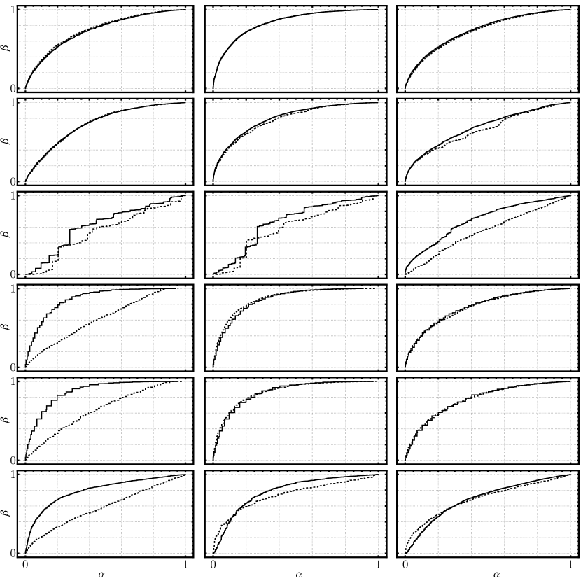
Figure S3: Comparison of ROC curves corresponding to $\|S_{n,k}\|_{1,w}$ (solid lines) and $T_{n,k}$ (dashed) for $n=10,k=5$, and various choices of $w,F$, and $G$. The three columns are associated with null distributions following $\operatorname{Uniform}[0,1],\mathcal{N}(0,1)$ and $\operatorname{Cauchy}(0,1)$, while the first and second set of three rows correspond to $Y\sim X+1$, and $Y\sim 1.1\cdot X$, respectively. Choices of $w$ are fixed row-wise, and read $w_{1}=\Phi^{-1},w_{2}(x)=x^{6},w_{3}=r_{\mu},w_{4}=\left(\Phi^{-1}\right)^{2},w_{5}(x)=(x-1/2)^{2},w_{6}=r_{\sigma}$, where $r_{\mu}$ and $r_{\sigma}$ are densities obtained from normalizing a Brownian motion on $[0,1]$.

For $G$ sufficiently close to $F$ (or $w^{\prime\prime}$ appropriately small), these error terms $\varepsilon_{S},\varepsilon_{T}$ are generally $O(1)$ compared to the $O(k)$ order of $R_{n,k}^{w}$, explaining the asymptotic equivalence of $\|\mathchoice{\mbox{\boldmath$S$}}{\mbox{\boldmath$S$}}{\mbox{\boldmath$\scriptstyle S$}}{\mbox{\boldmath$\scriptscriptstyle S$}}_{n,k}\|_{1,w}$ and $T_{n,k}^{w}$. Moreover, their similarity suggests that even in finite-sample regimes, $\|\mathchoice{\mbox{\boldmath$S$}}{\mbox{\boldmath$S$}}{\mbox{\boldmath$\scriptstyle S$}}{\mbox{\boldmath$\scriptscriptstyle S$}}_{n,k}\|_{1,w}$ and $T_{n,k}^{w}$ should generally behave comparably as long as $w$ is regular enough. We do not quantify this statement precisely, but demonstrate that it is borne out empirically in simulation studies like the one given in Supplementary Figure S3, where it is shown that, for fixed $n=10,k=5$, the ROC curves of $\|\mathchoice{\mbox{\boldmath$S$}}{\mbox{\boldmath$S$}}{\mbox{\boldmath$\scriptstyle S$}}{\mbox{\boldmath$\scriptscriptstyle S$}}_{n,k}\|_{1,w}$ and $T_{n,k}^{w}$ for various choices of $F,G$, $w$ (including highly irregular ones) match each other closely, indicating that the favorable power properties of $T_{n,k}^{w}$ [CJJ81] are expected to transfer to $\|\mathchoice{\mbox{\boldmath$S$}}{\mbox{\boldmath$S$}}{\mbox{\boldmath$\scriptstyle S$}}{\mbox{\boldmath$\scriptscriptstyle S$}}_{n,k}\|_{1,w}$ as well. Therefore, it is of interest to study the finite-sample distribution of $\|\mathchoice{\mbox{\boldmath$S$}}{\mbox{\boldmath$S$}}{\mbox{\boldmath$\scriptstyle S$}}{\mbox{\boldmath$\scriptscriptstyle S$}}_{n,k}\|_{1,w}$.

The main result of this section is the following characterization of the law of $\|\mathchoice{\mbox{\boldmath$S$}}{\mbox{\boldmath$S$}}{\mbox{\boldmath$\scriptstyle S$}}{\mbox{\boldmath$\scriptscriptstyle S$}}_{n,k}\|_{1,w}$. In what follows, we define $w_{j}=w(\frac{j-1}{k})$ and write $\mathchoice{\mbox{\boldmath$w$}}{\mbox{\boldmath$w$}}{\mbox{\boldmath$\scriptstyle w$}}{\mbox{\boldmath$\scriptscriptstyle w$}}\in\mathbb{R}^{k}$ to denote $(w_{1},\ldots,w_{k})$.

Theorem 1.

Let $\mathchoice{\mbox{\boldmath$w$}}{\mbox{\boldmath$w$}}{\mbox{\boldmath$\scriptstyle w$}}{\mbox{\boldmath$\scriptscriptstyle w$}}\in\mathbb{R}^{k}$ have pairwise distinct entries and $w_{\max}=\max_{j=1}^{k}|w_{j}|$. Then the Laplace transform of $\|\mathchoice{\mbox{\boldmath$S$}}{\mbox{\boldmath$S$}}{\mbox{\boldmath$\scriptstyle S$}}{\mbox{\boldmath$\scriptscriptstyle S$}}_{n,k}\|_{1,\mathchoice{\mbox{\boldmath$w$}}{\mbox{\boldmath$w$}}{\mbox{\boldmath$\scriptstyle w$}}{\mbox{\boldmath$\scriptscriptstyle w$}}}$ is given by

$$\mathbb{E}e^{t\|\mathchoice{\mbox{\boldmath$S$}}{\mbox{\boldmath$S$}}{\mbox{\boldmath$\scriptstyle S$}}{\mbox{\boldmath$\scriptscriptstyle S$}}_{n,k}\|_{1,\mathchoice{\mbox{\boldmath$w$}}{\mbox{\boldmath$w$}}{\mbox{\boldmath$\scriptstyle w$}}{\mbox{\boldmath$\scriptscriptstyle w$}}}}=(k-1)(-1)^{k+1}\cdot e^{tnw_{\max}}\times\sum_{j=1}^{k-1}a_{j}^{e^{t(w_{j}-w_{\max})}}\bigg{[}b_{n,k}\left(1-e^{t(w_{j}-w_{\max})(n+k-1)}\right)\\ +\sum_{m=0}^{k-3}c_{n,k,m}\left(1-e^{t(w_{j}-w_{\max})}\right)^{k-2-m}\bigg{]},$$ (4)

where for any $\mathchoice{\mbox{\boldmath$r$}}{\mbox{\boldmath$r$}}{\mbox{\boldmath$\scriptstyle r$}}{\mbox{\boldmath$\scriptscriptstyle r$}}\in\mathbb{R}^{k}$, $a_{j}^{\mathchoice{\mbox{\boldmath$r$}}{\mbox{\boldmath$r$}}{\mbox{\boldmath$\scriptstyle r$}}{\mbox{\boldmath$\scriptscriptstyle r$}}}=\prod_{m\neq j}(r_{j}-r_{m})^{-1}$ and

$$b_{n,k}=\frac{(-1)^{k}}{n+k-1}\cdot\binom{n+k-2}{k-2}^{-1}, c_{n,k,m}=\frac{(-1)^{m}}{n+1}\cdot\frac{\binom{k-2}{m}}{\binom{n+m+1}{m}}.$$

Remark 1.

For hypothesis testing, (4) needs to be inverted in order to recover the requisite null distribution. This can be done quickly and in a numerically stable manner, as we demonstrate in Supplementary Figure S4, where CDFs obtained from Monte Carlo iterates are contrasted with those computed from (4).

Remark 2.

The assumption that the components of $w$ are distinct is merely to simplify equation (4), and can be dropped. In case there are ties, the result is obtained by evaluating (4) along a sequence $\mathchoice{\mbox{\boldmath$w$}}{\mbox{\boldmath$w$}}{\mbox{\boldmath$\scriptstyle w$}}{\mbox{\boldmath$\scriptscriptstyle w$}}^{(n)}$ of weights whose entries are mutually distinct and converge to $w$. Explicit expressions (involving suitable partial derivatives of $a_{j}^{\mathchoice{\mbox{\boldmath$w$}}{\mbox{\boldmath$w$}}{\mbox{\boldmath$\scriptstyle w$}}{\mbox{\boldmath$\scriptscriptstyle w$}}}$ in each component of $w$) can be found in the Supplementary Material. Numerical inversions are performed without difficulty as before.

Theorem 1 enables hypothesis testing in regimes of $n$ and $k$ both remaining small, thereby complementing results of [HR80] where the asymptotic behavior of $\|\mathchoice{\mbox{\boldmath$S$}}{\mbox{\boldmath$S$}}{\mbox{\boldmath$\scriptstyle S$}}{\mbox{\boldmath$\scriptscriptstyle S$}}_{n,k}\|_{1,\mathchoice{\mbox{\boldmath$w$}}{\mbox{\boldmath$w$}}{\mbox{\boldmath$\scriptstyle w$}}{\mbox{\boldmath$\scriptscriptstyle w$}}}$ for $n,k\to\infty$, $k/n\to\alpha$ is considered. This leaves open the case of one parameter, say (without loss of generality) $n$, diverging towards $\infty$, with the other, $k$, kept fixed. With experimental methods producing ever more refined, yet possibly sparse, data, this situation is encountered increasingly often [HG09, YLG06, see, e.g.,]. The following result characterizes $\|\mathchoice{\mbox{\boldmath$S$}}{\mbox{\boldmath$S$}}{\mbox{\boldmath$\scriptstyle S$}}{\mbox{\boldmath$\scriptscriptstyle S$}}_{n,k}\|_{1,\mathchoice{\mbox{\boldmath$w$}}{\mbox{\boldmath$w$}}{\mbox{\boldmath$\scriptstyle w$}}{\mbox{\boldmath$\scriptscriptstyle w$}}}$ in this regime.

Theorem 2.

As $n\to\infty$ with $k$ remaining fixed, $\mathbb{P}\left(\|\mathchoice{\mbox{\boldmath$S$}}{\mbox{\boldmath$S$}}{\mbox{\boldmath$\scriptstyle S$}}{\mbox{\boldmath$\scriptscriptstyle S$}}_{n,k}\|_{1,\mathchoice{\mbox{\boldmath$w$}}{\mbox{\boldmath$w$}}{\mbox{\boldmath$\scriptstyle w$}}{\mbox{\boldmath$\scriptscriptstyle w$}}}\leq x\right)=\mathbb{P}\left(\|\mathchoice{\mbox{\boldmath$S$}}{\mbox{\boldmath$S$}}{\mbox{\boldmath$\scriptstyle S$}}{\mbox{\boldmath$\scriptscriptstyle S$}}_{k}\|_{1,\mathchoice{\mbox{\boldmath$w$}}{\mbox{\boldmath$w$}}{\mbox{\boldmath$\scriptstyle w$}}{\mbox{\boldmath$\scriptscriptstyle w$}}}\leq x\right)+\varepsilon(x)$, where $\mathchoice{\mbox{\boldmath$S$}}{\mbox{\boldmath$S$}}{\mbox{\boldmath$\scriptstyle S$}}{\mbox{\boldmath$\scriptscriptstyle S$}}_{k}\sim\operatorname{Dirichlet}(\mathbf{1}_{k})$ (with $\mathbf{1}_{k+1}\in\mathbb{Z}^{k}$ being the all-ones vector) is uniformly distributed on the $(k-1)$-dimensional simplex, and $\|\varepsilon\|_{\infty}\in O(n^{-1})$. Moreover, with $a_{j}^{\mathchoice{\mbox{\boldmath$w$}}{\mbox{\boldmath$w$}}{\mbox{\boldmath$\scriptstyle w$}}{\mbox{\boldmath$\scriptscriptstyle w$}}}$ as in Theorem 1,

$$\mathbb{P}\left(\|\mathchoice{\mbox{\boldmath$S$}}{\mbox{\boldmath$S$}}{\mbox{\boldmath$\scriptstyle S$}}{\mbox{\boldmath$\scriptscriptstyle S$}}_{k}\|_{1,\mathchoice{\mbox{\boldmath$w$}}{\mbox{\boldmath$w$}}{\mbox{\boldmath$\scriptstyle w$}}{\mbox{\boldmath$\scriptscriptstyle w$}}}\leq x\right)=(-1)^{k+1}\sum_{j=1}^{k-1}a_{j}^{\mathchoice{\mbox{\boldmath$w$}}{\mbox{\boldmath$w$}}{\mbox{\boldmath$\scriptstyle w$}}{\mbox{\boldmath$\scriptscriptstyle w$}}}\left[(x-w_{j})_{+}\right]^{k-1},$$ (5)

as long as the components of $w$ are pairwise distinct.

Remark 3.

As with Theorem 1, the distinctness assumption on $w$ can be relaxed by taking suitable limits.

3 The case $p>1$

The explicit form of Theorem 1 relies on the observation that $\mathchoice{\mbox{\boldmath$S$}}{\mbox{\boldmath$S$}}{\mbox{\boldmath$\scriptstyle S$}}{\mbox{\boldmath$\scriptscriptstyle S$}}_{n,k}\sim\operatorname{Multinomial}(n,\mathchoice{\mbox{\boldmath$S$}}{\mbox{\boldmath$S$}}{\mbox{\boldmath$\scriptstyle S$}}{\mbox{\boldmath$\scriptscriptstyle S$}}_{k})$ allows factorization of the Laplace transform of $\|\mathchoice{\mbox{\boldmath$S$}}{\mbox{\boldmath$S$}}{\mbox{\boldmath$\scriptstyle S$}}{\mbox{\boldmath$\scriptscriptstyle S$}}_{n,k}\|_{1,\mathchoice{\mbox{\boldmath$w$}}{\mbox{\boldmath$w$}}{\mbox{\boldmath$\scriptstyle w$}}{\mbox{\boldmath$\scriptscriptstyle w$}}}$: $\mathbb{E}e^{t\|\mathchoice{\mbox{\boldmath$S$}}{\mbox{\boldmath$S$}}{\mbox{\boldmath$\scriptstyle S$}}{\mbox{\boldmath$\scriptscriptstyle S$}}_{n,k}\|_{1,\mathchoice{\mbox{\boldmath$w$}}{\mbox{\boldmath$w$}}{\mbox{\boldmath$\scriptstyle w$}}{\mbox{\boldmath$\scriptscriptstyle w$}}}}=\mathbb{E}\|\mathchoice{\mbox{\boldmath$S$}}{\mbox{\boldmath$S$}}{\mbox{\boldmath$\scriptstyle S$}}{\mbox{\boldmath$\scriptscriptstyle S$}}_{k}\|_{1,e^{t\mathchoice{\mbox{\boldmath$w$}}{\mbox{\boldmath$w$}}{\mbox{\boldmath$\scriptstyle w$}}{\mbox{\boldmath$\scriptscriptstyle w$}}}}^{n}$. When $p>1$, interaction terms in $\|\mathchoice{\mbox{\boldmath$S$}}{\mbox{\boldmath$S$}}{\mbox{\boldmath$\scriptstyle S$}}{\mbox{\boldmath$\scriptscriptstyle S$}}_{n,k}\|_{p,\mathchoice{\mbox{\boldmath$w$}}{\mbox{\boldmath$w$}}{\mbox{\boldmath$\scriptstyle w$}}{\mbox{\boldmath$\scriptscriptstyle w$}}}^{p}$ prevent such a factorization. Nevertheless, the individual moments can still be accessed.

Theorem 3.

Let $G_{p}(x,y)=\sum_{m=0}^{\infty}\mathrm{Li}_{-pm}(x)y^{m}/m!$, where $\mathrm{Li}_{s}(x)=\sum_{j=1}^{\infty}j^{-s}x^{j}$ is the polylogarithm function. Denoting by $[x^{n}y^{m}]P(x,y)$ the $(n,m)^{\text{th}}$ coefficient of a formal power series $P$ in $x$ and $y$, we have

$$\mathbb{E}\left(\|\mathchoice{\mbox{\boldmath$S$}}{\mbox{\boldmath$S$}}{\mbox{\boldmath$\scriptstyle S$}}{\mbox{\boldmath$\scriptscriptstyle S$}}_{n,k}\|_{p,\mathchoice{\mbox{\boldmath$w$}}{\mbox{\boldmath$w$}}{\mbox{\boldmath$\scriptstyle w$}}{\mbox{\boldmath$\scriptscriptstyle w$}}}^{p}\right)^{m}=\dfrac{m!}{\binom{n+k-1}{k-1}}[x^{n}y^{m}]\prod_{i=1}^{k}G_{p}\left(x,w_{i}y\right).$$ (6)

In particular, the first $m$ moments of $\|\mathchoice{\mbox{\boldmath$S$}}{\mbox{\boldmath$S$}}{\mbox{\boldmath$\scriptstyle S$}}{\mbox{\boldmath$\scriptscriptstyle S$}}_{i,j}\|_{p,\mathchoice{\mbox{\boldmath$w$}}{\mbox{\boldmath$w$}}{\mbox{\boldmath$\scriptstyle w$}}{\mbox{\boldmath$\scriptscriptstyle w$}}}^{p}$ for $(i,j)\in\{0,\dots,n\}\times\{1,\dots,k\}$ can be computed in $O\left(nm\cdot(\log nm)\cdot k\right)$ time.

As with the $p=1$ case, there are three regimes of interest:

1. $n,k\to\infty$ while $k/n\to\alpha$;

2. $n,k$ both small; and

3. $n\to\infty$ with $k$ fixed.

Regime 1 is covered by the same central limit theorems in [HR80] that resolved the corresponding question when $p=1$. Theorem 3 will turn out to be useful primarily in regime 2, while the following analogue of Theorem 2 covers regime 3.

Theorem 4.

Let $Q_{p}(x)=\sum_{m=0}^{\infty}(pm)!x^{m}/m!$. Then for $n\to\infty$ with $k$ kept fixed, $\mathbb{P}(\|\mathchoice{\mbox{\boldmath$S$}}{\mbox{\boldmath$S$}}{\mbox{\boldmath$\scriptstyle S$}}{\mbox{\boldmath$\scriptscriptstyle S$}}_{n,k}\|_{p,\mathchoice{\mbox{\boldmath$w$}}{\mbox{\boldmath$w$}}{\mbox{\boldmath$\scriptstyle w$}}{\mbox{\boldmath$\scriptscriptstyle w$}}}^{p}\leq x)=\mathbb{P}\left(\|\mathchoice{\mbox{\boldmath$S$}}{\mbox{\boldmath$S$}}{\mbox{\boldmath$\scriptstyle S$}}{\mbox{\boldmath$\scriptscriptstyle S$}}_{k}\|_{p,\mathchoice{\mbox{\boldmath$w$}}{\mbox{\boldmath$w$}}{\mbox{\boldmath$\scriptstyle w$}}{\mbox{\boldmath$\scriptscriptstyle w$}}}^{p}\leq x\right)+\varepsilon(x)$, where $\|\varepsilon\|_{\infty}\in O(n^{-1})$, and

$$\mathbb{E}\left(\|\mathchoice{\mbox{\boldmath$S$}}{\mbox{\boldmath$S$}}{\mbox{\boldmath$\scriptstyle S$}}{\mbox{\boldmath$\scriptscriptstyle S$}}_{k}\|_{p,\mathchoice{\mbox{\boldmath$w$}}{\mbox{\boldmath$w$}}{\mbox{\boldmath$\scriptstyle w$}}{\mbox{\boldmath$\scriptscriptstyle w$}}}^{p}\right)^{m}=\dfrac{(k-1)!m!}{(pm+k-1)!}[x^{m}]\prod_{j=1}^{k}Q_{p}(w_{j}x).$$ (7)

In particular, the first $m$ moments of $\|\mathchoice{\mbox{\boldmath$S$}}{\mbox{\boldmath$S$}}{\mbox{\boldmath$\scriptstyle S$}}{\mbox{\boldmath$\scriptscriptstyle S$}}_{j}\|_{p,\mathchoice{\mbox{\boldmath$w$}}{\mbox{\boldmath$w$}}{\mbox{\boldmath$\scriptstyle w$}}{\mbox{\boldmath$\scriptscriptstyle w$}}}^{p}$ for $j\in\{1,\dots,k\}$ can be computed in$O(m\cdot(\log m)\cdot k)$ time.

Remark 4.

The generating function $Q_{p}(x)$ can be expressed as the generalized hypergeometric series $Q_{p}(x)={}_{p}F_{0}\big{[}1,\frac{1}{p},\frac{2}{p},\dots,\frac{p-1}{p}\big{]}(p^{2}x).$ In particular, for $p=2$ (i.e., including the Greenwood statistic $\|\mathchoice{\mbox{\boldmath$S$}}{\mbox{\boldmath$S$}}{\mbox{\boldmath$\scriptstyle S$}}{\mbox{\boldmath$\scriptscriptstyle S$}}_{k}\|_{2,\mathchoice{\mbox{\boldmath$1$}}{\mbox{\boldmath$1$}}{\mbox{\boldmath$\scriptstyle 1$}}{\mbox{\boldmath$\scriptscriptstyle 1$}}_{k}}^{2}$), we have $Q_{2}(x)={}_{2}F_{0}\big{[}1,\frac{1}{2}\big{]}(4x)=\frac{1}{\sqrt{x}}D\big{(}\frac{1}{2\sqrt{x}}\big{)}$, where Dawson’s integral

$$D(x)=e^{-x^{2}}\int_{0}^{x}e^{t^{2}}~{}\mathrm{d}t$$

is interpreted through its asymptotic expansion [AS65, cf.].

In order to perform hypothesis testing, Theorems 3 and 4 require numerical “inversion” similar to the need for inverse Laplace transforms to render (4) and (5) practical. More concretely, they require efficient reconstruction of a (compactly supported) distribution $F$ given its truncated moment sequence $\int x^{j}\ dF(x),j\in[m]$. Although this is a well-studied problem [Akh20, see], equations (6) and (7) have some unique properties that are not often encountered:

1. An arbitrary number of moments can be computed efficiently. This is markedly distinct from situations in which moments are estimated from, e.g., experimental observations and limited in number. Applying tools developed in this latter context [Sch20, Joh+07, ranging from extremal inequalities to maximum entropy based approaches to concretely applications-driven methods, see, e.g.,] typically under-utilizes all the information available, or becomes computationally infeasible.

2. Each moment can be computed exactly, and therefore usual concerns around the well-conditioning of the moment problem [Tal87, see, for example,] do not apply.

By exploiting these two properties, we can carry out the necessary reconstruction efficiently and with great accuracy, simply by considering expectations of Bernstein polynomials.

Proposition 1.

Let $X\in[0,1]$ be a random variable either (a) continuous with density $f\in C^{1}\left([0,1]\right)$, or (b) discrete with support $\mathrm{supp}_{X}=\{x_{0},\dots,x_{N}\}$, and $F$ be its CDF. Moreover, denote by $B_{n,x}$ the degree-$n$ Bernstein polynomial approximating $\mathbbm{1}_{[0,x]}$. Then, for any resolution $\varepsilon_{n}\to 0,\varepsilon_{n}>n^{-1/2}$, there exists $n_{0}(f,\varepsilon)\in\mathbb{N}$, so that for all $n\geq n_{0}$,

$$\sup_{x\in[0,1]}\big{|}\mathbb{E}B_{n,x}(X)-F(x)\big{|} \leq\frac{\|f\|_{\infty}+2\|f^{\prime}\|_{\infty}+2}{n+1},$$ (a)

$$\sup_{x\in[0,1]\setminus\mathrm{supp}_{X}^{\varepsilon_{n}}}\big{|}\mathbb{E}B_{n,x}(X)-F(x)\big{|} \leq e^{-2n\varepsilon_{n}^{2}},$$ (b)

where $\mathrm{supp}_{X}^{\varepsilon}=\left\{x\in[0,1]~{}:~{}d(x,\mathrm{supp}_{X})<\varepsilon\right\}$ is the $\varepsilon$-fattening of $\mathrm{supp}_{X}$.

Several features of the proposition are worth highlighting:

1. By virtue of $B_{n,x}$ being a degree-$n$ polynomial, $\mathbb{E}B_{n,x}(X)$ is just a linear combination of the first $n$ moments $\mu_{1},\ldots,\mu_{n}$ of $X$; more explicitly,

   $$\mathbb{E}B_{n,x}(X)=\sum_{m=0}^{\lfloor nx\rfloor}\binom{n}{m}(-1)^{n-m}\left(\delta^{n-m}\mu\right)_{m},$$

   where $\mu=\left(\mu_{j}\right)_{j\in\mathbb{N}}$ denotes the moment sequence of $X$, and $\delta$ is the difference operator.

2. For a discrete $X$ of $n$ atoms, $n$ moments are sufficient to determine the distribution of $X$ via solving an $n\times n$ Vandermonde system, which can be performed in $O(n^{2})$ time [BP70]. However, $\|\mathchoice{\mbox{\boldmath$S$}}{\mbox{\boldmath$S$}}{\mbox{\boldmath$\scriptstyle S$}}{\mbox{\boldmath$\scriptscriptstyle S$}}_{n,k}\|_{p,\mathchoice{\mbox{\boldmath$w$}}{\mbox{\boldmath$w$}}{\mbox{\boldmath$\scriptstyle w$}}{\mbox{\boldmath$\scriptscriptstyle w$}}}^{p}$ generically has $O(n^{k-1})$ atoms, whose precise locations within $\{x_{\min},\dots,\|\mathchoice{\mbox{\boldmath$w$}}{\mbox{\boldmath$w$}}{\mbox{\boldmath$\scriptstyle w$}}{\mbox{\boldmath$\scriptscriptstyle w$}}\|_{\infty}n^{p}\}$ are typically unknown, therefore requiring $O(\min\{\|\mathchoice{\mbox{\boldmath$w$}}{\mbox{\boldmath$w$}}{\mbox{\boldmath$\scriptstyle w$}}{\mbox{\boldmath$\scriptscriptstyle w$}}\|_{\infty}^{2}n^{2p},n^{2(k-1)}\})$ operations, which is prohibitively large even for small values of $p$ or $k$.

3. $B_{n,x}$ may be replaced with any other polynomial approximation scheme in order to impose desired properties on the reconstructed density. For instance, if the user wishes to perform a one-sided test, then resorting to one-sided polynomial approximations [BQM12, the optimal of which is worked out in] is more suitable.

Beyond its practical impact in performing two-sample tests when $n$ is large and $k$ modest, the quantity $\|\mathchoice{\mbox{\boldmath$S$}}{\mbox{\boldmath$S$}}{\mbox{\boldmath$\scriptstyle S$}}{\mbox{\boldmath$\scriptscriptstyle S$}}_{k}\|_{p,\mathchoice{\mbox{\boldmath$w$}}{\mbox{\boldmath$w$}}{\mbox{\boldmath$\scriptstyle w$}}{\mbox{\boldmath$\scriptscriptstyle w$}}}^{p}$ appearing in Theorems 2 and 4 is of independent interest in the context of one-sample testing, where it constitutes the appropriate equivalent of $\|\mathchoice{\mbox{\boldmath$S$}}{\mbox{\boldmath$S$}}{\mbox{\boldmath$\scriptstyle S$}}{\mbox{\boldmath$\scriptscriptstyle S$}}_{n,k}\|_{p,\mathchoice{\mbox{\boldmath$w$}}{\mbox{\boldmath$w$}}{\mbox{\boldmath$\scriptstyle w$}}{\mbox{\boldmath$\scriptscriptstyle w$}}}^{p}$. The case of Greenwood’s statistic (corresponding to $p=2$ and $\mathchoice{\mbox{\boldmath$w$}}{\mbox{\boldmath$w$}}{\mbox{\boldmath$\scriptstyle w$}}{\mbox{\boldmath$\scriptscriptstyle w$}}=\mathbf{1}_{k}$) has received particular attention, with extensive studies clarifying left-tail behaviour, asymptotic normality as $k\to\infty$, and large deviation functions. Theorem 4 can be used to supplement these results with a characterization of the right tail.

Proposition 2.

Without loss of generality, assume $\mathchoice{\mbox{\boldmath$w$}}{\mbox{\boldmath$w$}}{\mbox{\boldmath$\scriptstyle w$}}{\mbox{\boldmath$\scriptscriptstyle w$}}\in\mathbb{R}_{+}^{k+1}$ and $\|\mathchoice{\mbox{\boldmath$w$}}{\mbox{\boldmath$w$}}{\mbox{\boldmath$\scriptstyle w$}}{\mbox{\boldmath$\scriptscriptstyle w$}}\|_{\infty}=1$, and denote by

$$W_{\mathchoice{\mbox{\boldmath$w$}}{\mbox{\boldmath$w$}}{\mbox{\boldmath$\scriptstyle w$}}{\mbox{\boldmath$\scriptscriptstyle w$}}}=\left|\{1\leq j\leq k+1~{}:~{}w_{j}=1\}\right|$$

the number of weight components assuming value $1$. Then the density $f_{k}^{p,\mathchoice{\mbox{\boldmath$w$}}{\mbox{\boldmath$w$}}{\mbox{\boldmath$\scriptstyle w$}}{\mbox{\boldmath$\scriptscriptstyle w$}}}$ of $\|\mathchoice{\mbox{\boldmath$S$}}{\mbox{\boldmath$S$}}{\mbox{\boldmath$\scriptstyle S$}}{\mbox{\boldmath$\scriptscriptstyle S$}}_{k}\|_{p,\mathchoice{\mbox{\boldmath$w$}}{\mbox{\boldmath$w$}}{\mbox{\boldmath$\scriptstyle w$}}{\mbox{\boldmath$\scriptscriptstyle w$}}}^{p}$ is analytic on $[x_{0},1]$, where

$$x_{0}=\begin{cases}\frac{1}{2^{p-1}},&\text{if\, $W_{\mathchoice{\mbox{\boldmath$w$}}{\mbox{\boldmath$w$}}{\mbox{\boldmath$\scriptstyle w$}}{\mbox{\boldmath$\scriptscriptstyle w$}}}=k+1$},\\ \max_{j:w_{j}<1}w_{j},&\text{otherwise},\end{cases}$$

and its degree-$r$ Taylor polynomial around $1$ can be computed in $O\left(\frac{r}{p}\log\frac{r}{p}\log k+[r\log r]^{2}\right)$ time. For $r=k-2$ it reads

$$f_{k}^{p,\mathchoice{\mbox{\boldmath$w$}}{\mbox{\boldmath$w$}}{\mbox{\boldmath$\scriptstyle w$}}{\mbox{\boldmath$\scriptscriptstyle w$}}}(x)=\dfrac{(k-1)W_{\mathchoice{\mbox{\boldmath$w$}}{\mbox{\boldmath$w$}}{\mbox{\boldmath$\scriptstyle w$}}{\mbox{\boldmath$\scriptscriptstyle w$}}}}{2^{k-1}}\left(1-x\right)^{k-2}+O\left((1-x)^{k-1}\right).$$

In particular, Greenwood’s statistic satisfies

$$f_{k}^{2,\mathbf{1}_{k}}(x)=\dfrac{\binom{k}{2}}{2^{k-2}}\left(1-x\right)^{k-2}+O\left((1-x)^{k-1}\right).$$

The right tail is typically the one of interest in one- and two-sample tests, and so as long as long as the desired significance threshold $\alpha$ is less than $\mathbb{P}\left(\|\mathchoice{\mbox{\boldmath$S$}}{\mbox{\boldmath$S$}}{\mbox{\boldmath$\scriptstyle S$}}{\mbox{\boldmath$\scriptscriptstyle S$}}_{k}\|_{p,\mathchoice{\mbox{\boldmath$w$}}{\mbox{\boldmath$w$}}{\mbox{\boldmath$\scriptstyle w$}}{\mbox{\boldmath$\scriptscriptstyle w$}}}^{p}\geq x_{0}\right)$, Proposition 2 allows for calculating $\varepsilon$-accurate $p$-values in $O(\log^{2}\varepsilon)$ time. This compares favorably with the $O\left(\varepsilon^{-1}\right)$ rate of Theorem 4, and can provide a substantial speed-up for large data sets.

4 Hypothesis testing when $|\mathcal{A}|>1$

Assume without loss of generality that $X\sim\operatorname{Uniform}([0,1])$ and $Y$ has density $g(x)=1+h(x)/\sqrt{n}$. In the case of singleton hypotheses $F=F^{*}$ and $G\in\{F^{*},G^{*}\}$, $\|\mathchoice{\mbox{\boldmath$S$}}{\mbox{\boldmath$S$}}{\mbox{\boldmath$\scriptstyle S$}}{\mbox{\boldmath$\scriptscriptstyle S$}}_{n,k}\|_{1,\mathchoice{\mbox{\boldmath$h$}}{\mbox{\boldmath$h$}}{\mbox{\boldmath$\scriptstyle h$}}{\mbox{\boldmath$\scriptscriptstyle h$}}}$ can be regarded as a non-parametric version of the likelihood ratio test for alternatives $G$ that are near $F$. This follows from the asymptotic equivalence between tests based on $\|\mathchoice{\mbox{\boldmath$S$}}{\mbox{\boldmath$S$}}{\mbox{\boldmath$\scriptstyle S$}}{\mbox{\boldmath$\scriptscriptstyle S$}}_{n,k}\|_{1,\mathchoice{\mbox{\boldmath$w$}}{\mbox{\boldmath$w$}}{\mbox{\boldmath$\scriptstyle w$}}{\mbox{\boldmath$\scriptscriptstyle w$}}}$ and likelihood-ratio tests [Hol72], and can also be seen by observing that

$$\frac{\sqrt{n}}{n+k}\log\prod_{j=1}^{n}g(Y_{j})=\frac{\sqrt{n}}{n+k}\sum_{j=1}^{n}\log\left[1+\frac{h(Y_{j})}{\sqrt{n}}\right]\approx\frac{1}{n+k}\sum_{j=1}^{n}h(Y_{j})\approx\sum_{j=1}^{k}h\left(\frac{j-1}{k}\right)S_{n,k}(j)=\|\mathchoice{\mbox{\boldmath$S$}}{\mbox{\boldmath$S$}}{\mbox{\boldmath$\scriptstyle S$}}{\mbox{\boldmath$\scriptscriptstyle S$}}_{n,k}\|_{1,\mathchoice{\mbox{\boldmath$h$}}{\mbox{\boldmath$h$}}{\mbox{\boldmath$\scriptstyle h$}}{\mbox{\boldmath$\scriptscriptstyle h$}}},$$

where $\mathchoice{\mbox{\boldmath$h$}}{\mbox{\boldmath$h$}}{\mbox{\boldmath$\scriptstyle h$}}{\mbox{\boldmath$\scriptscriptstyle h$}}\in\mathbb{R}^{k+1}$ has $j^{\text{th}}$ component $h\left((j-1)/k\right)$.

By analogous reasoning, if the alternative hypothesis $G\in\big{\{}1+h^{\theta}(x)/\sqrt{n}\big{\}}_{\theta\in\Theta}$ is composite (and parameterized by $\theta$ over some index set $\Theta$), then given observations $X_{1},\ldots,X_{k-1}$ and $Y_{1},\ldots,Y_{n}$, one may expect tests based on $\sup_{\theta\in\Theta}\|\mathchoice{\mbox{\boldmath$S$}}{\mbox{\boldmath$S$}}{\mbox{\boldmath$\scriptstyle S$}}{\mbox{\boldmath$\scriptscriptstyle S$}}_{n,k}\|_{1,\mathchoice{\mbox{\boldmath$h$}}{\mbox{\boldmath$h$}}{\mbox{\boldmath$\scriptstyle h$}}{\mbox{\boldmath$\scriptscriptstyle h$}}^{\theta}}$ to provide non-parametric equivalents of generalized likelihood-ratio tests. When $|\Theta|=m<\infty$, multivariate extensions of the previous results follow in a straightforward manner.

Proposition 3.

For $m$ weights $\mathchoice{\mbox{\boldmath$w$}}{\mbox{\boldmath$w$}}{\mbox{\boldmath$\scriptstyle w$}}{\mbox{\boldmath$\scriptscriptstyle w$}}^{1},\ldots,\mathchoice{\mbox{\boldmath$w$}}{\mbox{\boldmath$w$}}{\mbox{\boldmath$\scriptstyle w$}}{\mbox{\boldmath$\scriptscriptstyle w$}}^{m}\in\mathbb{R}^{k}$, each with pairwise distinct entries, the Laplace transform of the tuple $S_{(m)}=\left(\|\mathchoice{\mbox{\boldmath$S$}}{\mbox{\boldmath$S$}}{\mbox{\boldmath$\scriptstyle S$}}{\mbox{\boldmath$\scriptscriptstyle S$}}_{n,k}\|_{1,\mathchoice{\mbox{\boldmath$w$}}{\mbox{\boldmath$w$}}{\mbox{\boldmath$\scriptstyle w$}}{\mbox{\boldmath$\scriptscriptstyle w$}}^{1}},\ldots,\|\mathchoice{\mbox{\boldmath$S$}}{\mbox{\boldmath$S$}}{\mbox{\boldmath$\scriptstyle S$}}{\mbox{\boldmath$\scriptscriptstyle S$}}_{n,k}\|_{1,\mathchoice{\mbox{\boldmath$w$}}{\mbox{\boldmath$w$}}{\mbox{\boldmath$\scriptstyle w$}}{\mbox{\boldmath$\scriptscriptstyle w$}}^{m}}\right)$ is given by

$$\mathbb{E}e^{\langle t,S_{(m)}\rangle}=(k-1)(-1)^{k+1}\cdot e^{nw^{\max}}\sum_{j=1}^{k-1}a_{j}^{e^{\omega_{j}}}\bigg{[}b_{n,k}\left(1-e^{\omega_{j}(n+k-2)}\right)+\sum_{m=0}^{k-3}c_{n,k,m}\left(1-e^{\omega_{j}}\right)^{k-1-m}\bigg{]},$$

where $t=(t_{1},\ldots,t_{m})$, $\omega_{j}=\sum_{r=1}^{m}t_{r}w_{j}^{r}-w^{\max}$ with $w^{\max}=\max_{j}\sum_{r=1}^{m}t_{r}w^{r}_{j}$, and $a_{j}^{w},b_{n,k}$ and $c_{n,k,m}$ are defined as in Theorem 1.

Moreover, the joint moments of $S_{(m)}$ can be computed in $O\big{(}n\prod_{j=1}^{r}m_{j}$ $\times(\log n\prod_{j=1}^{r}m_{j})\times k\big{)}$ time as

$$\mathbb{E}\prod_{j=1}^{r}\left(\|\mathchoice{\mbox{\boldmath$S$}}{\mbox{\boldmath$S$}}{\mbox{\boldmath$\scriptstyle S$}}{\mbox{\boldmath$\scriptscriptstyle S$}}_{n,k}\|_{p_{j},\mathchoice{\mbox{\boldmath$w$}}{\mbox{\boldmath$w$}}{\mbox{\boldmath$\scriptstyle w$}}{\mbox{\boldmath$\scriptscriptstyle w$}}^{j}}^{p_{j}}\right)^{m_{j}}=\dfrac{\prod_{j=1}^{r}m_{j}!}{\binom{n+k-1}{k-1}}[x^{n}y_{1}^{m_{1}}\cdots y_{r}^{m_{r}}]\prod_{i=1}^{k}G_{r}\left(x,w^{1}_{i}y_{1},\dots,w^{r}_{i}y_{r}\right),$$

where $G_{r}(x,y_{1},\dots,y_{r})=\sum_{m_{1},\dots,m_{r}=0}^{\infty}\mathrm{Li}_{-\sum_{j=1}^{r}p_{j}m_{j}}(x)\prod_{j=1}^{r}y_{j}^{m}/m_{j}!$. These joint moments can be used to approximate $\mathbb{P}\left(\|S_{(m)}\|_{\infty}\leq x\right)$ up to $\varepsilon$ accuracy in $O\left(\varepsilon^{-1}\right)$ time.

Part of the motivation for formulating Proposition 3 is to improve the performance of non-parametric testing procedures in the context of scale alternatives. As noted earlier, for location families, the weight functions $w_{1}^{\mu}(x)=x$ and $w_{2}^{\mu}(x)=\Phi^{-1}(x)$, where $\Phi$ denotes the standard Gaussian CDF, are known to compare impressively against the parametric $t$-test when alternatives $G_{n}$ are shifts of $F$, with Pitman efficiencies never dropping below $\approx 0.86$ and $1$, respectively [HL56]. However, for scale families, the corresponding choices $w_{1}^{\sigma}(x)=(x-1/2)^{2}$ and $w_{2}^{\sigma}(x)=\Phi^{-1}(x)^{2}$ [AB60] compare less favorably against the relevant $F$-test: [Suk57] demonstrated that $\inf_{F}e_{w_{1}^{\sigma}}^{\sigma}(F)=0$ (where $e_{w_{1}^{\sigma}}^{\sigma}(F)$ denotes the Pitman efficiency of $\|\mathchoice{\mbox{\boldmath$S$}}{\mbox{\boldmath$S$}}{\mbox{\boldmath$\scriptstyle S$}}{\mbox{\boldmath$\scriptscriptstyle S$}}_{n,k}\|_{1,\mathchoice{\mbox{\boldmath$w$}}{\mbox{\boldmath$w$}}{\mbox{\boldmath$\scriptstyle w$}}{\mbox{\boldmath$\scriptscriptstyle w$}}_{1}^{\sigma}}$ against the $F$-test under scale shifts) under $X\sim F$, while [Klo62] showed that $\inf_{F}e_{w_{2}^{\sigma}}^{\sigma}(F)\leq 0.47$ and conjectured that, in fact, efficiencies arbitrarily close to zero can be realized. The following example confirms a considerably stronger version of Klotz’ conjecture.

Proposition 4.

For $a,b>0$, define random variables $X_{a,b}$ through their densities

$$f_{a,b}(x)=\frac{1}{Z}\times\begin{cases}\frac{1}{a}\frac{x+b}{b-a},&\text{if }-b\leq x<-a,\\ -\frac{1}{x},&\text{if }-a\leq x<-1,\\ 1,&\text{if }-1\leq x<1,\\ \frac{1}{x},&\text{if }1\leq x<a,\\ \frac{1}{a}\frac{x-b}{a-b},&\text{if }a\leq x<b,\end{cases}$$

where $Z=2\log a+1+\kappa$, with $\kappa=b/a$. Then, as $a\to\infty$ while keeping $\kappa\in o(\log a)$, $e_{w}^{\sigma}(F_{a,b})\to 0$ for any $w\in\mathcal{C}^{1}([0,1])$ whose derivative is bounded by $C[x^{-1}|\log x|^{p}+\break(1-x)^{-1}|\log(1-x)|^{p}]$ for some constants $C>0$ and $p>0$.

If it is unknown whether the data-generating mechanism for $X_{1},\ldots,X_{k}$ lies within distributions against which weights like $w_{2}^{\sigma}$ are powerful (which includes most named distributions, see [Klo62] and Example 1 in the Supplementary Material), or is closer to the one described in Proposition 4, then combining $w_{2}^{\sigma}$ with a complementary weight function in the manner outlined by Proposition 3 may boost performance.

5 Application to non-parametric hypothesis tests

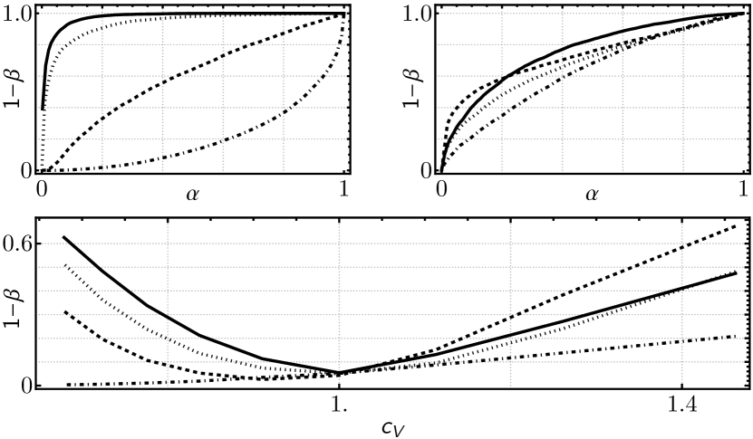
Figure 1: One-sample test comparison between Greenwood’s $\|\mathchoice{\mbox{\boldmath$S$}}{\mbox{\boldmath$S$}}{\mbox{\boldmath$\scriptstyle S$}}{\mbox{\boldmath$\scriptscriptstyle S$}}_{k}\|_{2,\mathbf{1}_{k}}^{2}$ (solid line), Cox and Oakes’ $CO_{k}$ (dashed), Gail and Gastwirth’ $G_{k}$ (dotted), and the Cramér-von Mises test (dot-dashed) for $k=20$. Upper panels display ROC curves of type-I error ($\alpha$) against power ($1-\beta$) in the case of under- and over-dispersed alternatives (left and right), respectively. Bottom panel illustrates power against varying coefficient of variation $c_{V}$.

We begin by carrying out the original test of uniformity proposed by [Gre46] for moderately sized $k=20$ (which does not yet induce CLT-type behavior) and comparing it to three other common tests. This analysis extends previous power studies that either omitted Greenwood’s statistic for lack of exact $z$-scores, or accepted approximation errors in their results [DAg86, HM05, e.g.,]. Despite the small scale of our comparison, the results are promising, and we hope they will encourage inclusion of Greenwood’s statistic into future benchmarking efforts.

[Gre46] was interested in testing under- or over-dispersion of spacings relative to a homogeneous Poisson Point Process; that is, he considered the hypotheses

$$\mathcal{H}_{0}:\left\{T_{j}\right\}_{j\in[k]}\stackrel{{\scriptstyle\text{i.i.d.}}}{{\sim}}\text{Exp}(\lambda), \mathcal{H}_{1}:\left\{T_{j}\right\}_{j\in[k]}\stackrel{{\scriptstyle\text{i.i.d.}}}{{\sim}}X,\text{ where }c_{V}^{2}=\frac{\mathrm{Var}X}{\left(\mathbb{E}X\right)^{2}}\neq 1,$$

which is equivalent to testing whether $(T_{1},T_{2},\dots,T_{k})/\sum_{j=1}^{k}T_{j}$ is distributed like $\mathchoice{\mbox{\boldmath$S$}}{\mbox{\boldmath$S$}}{\mbox{\boldmath$\scriptstyle S$}}{\mbox{\boldmath$\scriptscriptstyle S$}}_{k}$ under the null. Greenwood proposed to use $\|\mathchoice{\mbox{\boldmath$S$}}{\mbox{\boldmath$S$}}{\mbox{\boldmath$\scriptstyle S$}}{\mbox{\boldmath$\scriptscriptstyle S$}}_{k}\|_{2,\mathbf{1}_{k}}^{2}$, but was not able to quantify its power, numerically or otherwise. Theorem 4 and Proposition 1 allow to compute the law of Greenwood’s statistics quickly (computing $p$-values of $10,000$ simulation runs each with $k\leq 30$ takes $\approx 5$ seconds on an ordinary laptop), facilitating power comparisons.

The test statistics we compared against were $CO_{k}$ from [CO18], $\mathchoice{\mbox{\boldmath$S$}}{\mbox{\boldmath$S$}}{\mbox{\boldmath$\scriptstyle S$}}{\mbox{\boldmath$\scriptscriptstyle S$}}_{k}$ from [GG78], and the Cramér-von Mises test. [HM05] identified these as high-performing goodness-of-fit tests through extensive simulation studies. We compared them to Greenwood’s statistic on the same under- and over-dispersed alternatives used in [HM05]: the uniform distribution on $[0,1]$, and the Weibull distribution of scale $1$ and shape $0.8$. The results, together with a sensitivity analysis of power against varying dispersion (using the family of Weibull distributions of scale $1$ and shapes $0.8,0.9,\dots,1.5$), are displayed in Figure 1. They reveal competitive performance of $\|\mathchoice{\mbox{\boldmath$S$}}{\mbox{\boldmath$S$}}{\mbox{\boldmath$\scriptstyle S$}}{\mbox{\boldmath$\scriptscriptstyle S$}}_{k}\|_{2,\mathbf{1}_{k}}^{2}$, especially in the under-dispersed regime (upper-left).

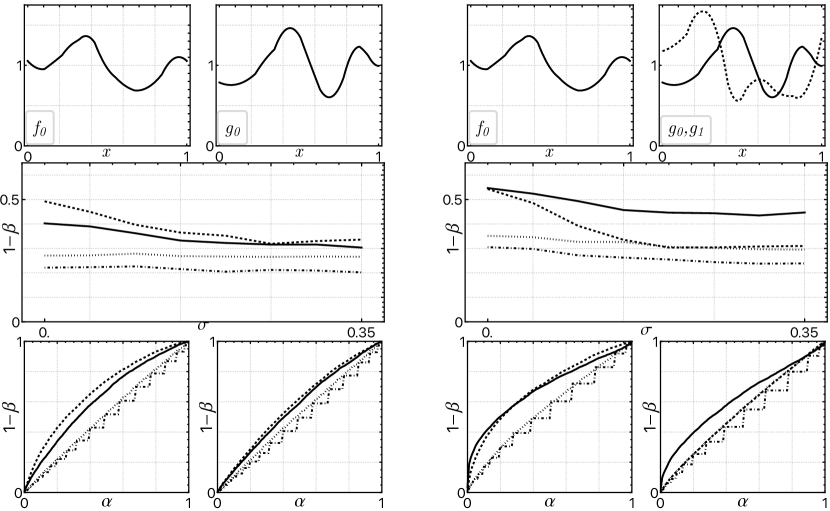
Figure 2: Two-sample test comparisons (center and bottom row) of $\|\mathchoice{\mbox{\boldmath$S$}}{\mbox{\boldmath$S$}}{\mbox{\boldmath$\scriptstyle S$}}{\mbox{\boldmath$\scriptscriptstyle S$}}_{n,k}\|_{1,\mathchoice{\mbox{\boldmath$h$}}{\mbox{\boldmath$h$}}{\mbox{\boldmath$\scriptstyle h$}}{\mbox{\boldmath$\scriptscriptstyle h$}}}$ (solid line), the likelihood-ratio statistic (dashed), Mann-Whitney’s U statistic (dotted), and the Kolmogorov-Smirnov statistic (dot-dashed) on $\mathcal{N}$ and $\mathcal{A}$ centered around given distributions (top row). $(1-\beta)$ and $\alpha$ denote power and test size as in Figure 1, and $\sigma$ the measurement noise. Plots in the middle row correspond to $\alpha=0.05$. In each scenario, ROC curves in the bottom row correspond to $\sigma=0$ and $0.3$, respectively. All simulations were run on $n=50,k=25$ and $10,000$ Monte-Carlo iterations.

To empirically probe the relevance of Theorem 1 and the multiple testing strategy presented in the previous section, we compared power properties of $\|\mathchoice{\mbox{\boldmath$S$}}{\mbox{\boldmath$S$}}{\mbox{\boldmath$\scriptstyle S$}}{\mbox{\boldmath$\scriptscriptstyle S$}}_{n,k}\|_{1,\mathchoice{\mbox{\boldmath$h$}}{\mbox{\boldmath$h$}}{\mbox{\boldmath$\scriptstyle h$}}{\mbox{\boldmath$\scriptscriptstyle h$}}}$ and $\max\{\|\mathchoice{\mbox{\boldmath$S$}}{\mbox{\boldmath$S$}}{\mbox{\boldmath$\scriptstyle S$}}{\mbox{\boldmath$\scriptscriptstyle S$}}_{n,k}\|_{1,\mathchoice{\mbox{\boldmath$h$}}{\mbox{\boldmath$h$}}{\mbox{\boldmath$\scriptstyle h$}}{\mbox{\boldmath$\scriptscriptstyle h$}}_{0}},\|\mathchoice{\mbox{\boldmath$S$}}{\mbox{\boldmath$S$}}{\mbox{\boldmath$\scriptstyle S$}}{\mbox{\boldmath$\scriptscriptstyle S$}}_{n,k}\|_{1,\mathchoice{\mbox{\boldmath$h$}}{\mbox{\boldmath$h$}}{\mbox{\boldmath$\scriptstyle h$}}{\mbox{\boldmath$\scriptscriptstyle h$}}_{1}}\}$ against the gLRT, as well as against two omnibus tests [Kol33, MW47] which are widely used in practice. Results are shown in Figure 2, with simple and composite cases divided into left and right column, respectively; and null ($f_{0}$) and alternative ($g_{0}=1+h_{0}/\sqrt{n},g_{1}=1+h_{1}/\sqrt{n}$) distributions were chosen to reflect fairly generic multi-modal two-sample setups (top row). In order to simulate “measurement noise” or misspecification of $F$ and $G$ around $f_{0},g_{0}$ and $g_{1}$, $\mathscr{X}_{k}$ and $\mathscr{Y}_{n}$ samples were perturbed by Gaussian noise of varying standard deviation $\sigma\in[0,0.35]$, and power for the (generalized) likelihood-ratio statistic, its $\|\mathchoice{\mbox{\boldmath$S$}}{\mbox{\boldmath$S$}}{\mbox{\boldmath$\scriptstyle S$}}{\mbox{\boldmath$\scriptscriptstyle S$}}_{n,k}\|_{1,\mathchoice{\mbox{\boldmath$h$}}{\mbox{\boldmath$h$}}{\mbox{\boldmath$\scriptstyle h$}}{\mbox{\boldmath$\scriptscriptstyle h$}}}$ counterparts, and the two omnibus tests was computed at size $\alpha=0.05$ (center row of Figure 2). As expected, the likelihood-ratio dominates in the noiseless regime. However, $\|\mathchoice{\mbox{\boldmath$S$}}{\mbox{\boldmath$S$}}{\mbox{\boldmath$\scriptstyle S$}}{\mbox{\boldmath$\scriptscriptstyle S$}}_{n,k}\|_{1,\mathchoice{\mbox{\boldmath$h$}}{\mbox{\boldmath$h$}}{\mbox{\boldmath$\scriptstyle h$}}{\mbox{\boldmath$\scriptscriptstyle h$}}}$ and its generalized extension perform competitively, closing the gap to likelihood ratio tests (or in the case of composite alternatives, reversing it) as noise is introduced. Importantly, calibrating likelihood-ratio tests in these contexts requires exact knowledge of the perturbation (which in general is not accessible to the practitioner), while tests based on $\|\mathchoice{\mbox{\boldmath$S$}}{\mbox{\boldmath$S$}}{\mbox{\boldmath$\scriptstyle S$}}{\mbox{\boldmath$\scriptscriptstyle S$}}_{n,k}\|_{1,\mathchoice{\mbox{\boldmath$h$}}{\mbox{\boldmath$h$}}{\mbox{\boldmath$\scriptstyle h$}}{\mbox{\boldmath$\scriptscriptstyle h$}}}$ do not. A more thorough description of the various compared tests for all sizes and fixed $\sigma=0$ and $\sigma=0.3$ is provided in the ROC curves of Figure 2 (bottom row), which confirm that the favorable performance of $\|\mathchoice{\mbox{\boldmath$S$}}{\mbox{\boldmath$S$}}{\mbox{\boldmath$\scriptstyle S$}}{\mbox{\boldmath$\scriptscriptstyle S$}}_{n,k}\|_{1,\mathchoice{\mbox{\boldmath$h$}}{\mbox{\boldmath$h$}}{\mbox{\boldmath$\scriptstyle h$}}{\mbox{\boldmath$\scriptscriptstyle h$}}}$ persists across the range of $\alpha$ most relevant in practice.

Although we find the theoretical and simulation evidence presented here convincing, this alone is not enough to ensure that our results will be utilized elsewhere. To aid practitioners in applying our methods, we provide code implementing most of the functionality outlined in this manuscript at https://github.com/songlab-cal/mochis (currently as a Mathematica notebook, but python and R packages are forthcoming). Its interface allows users to specify $f_{0}$ and any number of $g_{i}\in\mathcal{A}$ on a bounded interval or $\mathbb{R}$ through either a simple drag-and-drop mechanism or explicitly in closed or numerical form. From there, the relevant distribution of $\|\mathchoice{\mbox{\boldmath$S$}}{\mbox{\boldmath$S$}}{\mbox{\boldmath$\scriptstyle S$}}{\mbox{\boldmath$\scriptscriptstyle S$}}_{n,k}\|^{p}_{p,\mathchoice{\mbox{\boldmath$w$}}{\mbox{\boldmath$w$}}{\mbox{\boldmath$\scriptstyle w$}}{\mbox{\boldmath$\scriptscriptstyle w$}}}$ (in the case of $p=1$) or moments ($p>1$) are directly computed, and $p$-values corresponding to a given set of samples $X_{1},\ldots,X_{k}$, $Y_{1},\ldots,Y_{n}$ calculated. Optional arguments allow customization of any part of the procedure. Even though the current implementation focuses on the one- and two-sample situations described above, several generalizations are straightforward to include:

1. When extending results from continuous variables to discrete ones, ties can be resolved uniformly at random when constructing $\mathchoice{\mbox{\boldmath$S$}}{\mbox{\boldmath$S$}}{\mbox{\boldmath$\scriptstyle S$}}{\mbox{\boldmath$\scriptscriptstyle S$}}_{n,k}$ from $X_{1},\ldots,X_{k}$ and $Y_{1},\ldots,Y_{n}$.

2. The i.i.d. assumption on $X_{1},\ldots,X_{k}$ and $Y_{1},\ldots,Y_{n}$ can be relaxed to any other setting where null distributions effectively reduce to uniform samples from the discrete or continuous simplex; e.g., the same reasoning applies to paired two-sample tests.

3. Several representative weight choices corresponding to commonly encountered alternatives (e.g., $\mathchoice{\mbox{\boldmath$w$}}{\mbox{\boldmath$w$}}{\mbox{\boldmath$\scriptstyle w$}}{\mbox{\boldmath$\scriptscriptstyle w$}}=(k,k-1,\ldots,0)$ associated with Mann-Whitney’s $U$ statistic in the case of $Y$ stochastically dominating or being stochastically dominated by $X$) are included in the code base as pre-computed tables for the case of $p=1$ due to their relevance in two-sample testing. An interface allows users to specify similar generic weight choices (not necessarily arising from any fixed $f_{0}$ and $g_{0}$) for both $p=1$ and $p>1$ (which can become relevant for non-i.i.d. data).

4. The hypothesis testing results derived here only relied on the moments of $\|\mathchoice{\mbox{\boldmath$S$}}{\mbox{\boldmath$S$}}{\mbox{\boldmath$\scriptstyle S$}}{\mbox{\boldmath$\scriptscriptstyle S$}}_{k}\|_{p,\mathchoice{\mbox{\boldmath$w$}}{\mbox{\boldmath$w$}}{\mbox{\boldmath$\scriptstyle w$}}{\mbox{\boldmath$\scriptscriptstyle w$}}}^{p}$ and $\|\mathchoice{\mbox{\boldmath$S$}}{\mbox{\boldmath$S$}}{\mbox{\boldmath$\scriptstyle S$}}{\mbox{\boldmath$\scriptscriptstyle S$}}_{n,k}\|_{p,\mathchoice{\mbox{\boldmath$w$}}{\mbox{\boldmath$w$}}{\mbox{\boldmath$\scriptstyle w$}}{\mbox{\boldmath$\scriptscriptstyle w$}}}^{p}$ to reconstruct $\mathbb{E}\left[\mathbbm{1}_{[0,t]}\left(\|\mathchoice{\mbox{\boldmath$S$}}{\mbox{\boldmath$S$}}{\mbox{\boldmath$\scriptstyle S$}}{\mbox{\boldmath$\scriptscriptstyle S$}}_{k}\|_{p,\mathchoice{\mbox{\boldmath$w$}}{\mbox{\boldmath$w$}}{\mbox{\boldmath$\scriptstyle w$}}{\mbox{\boldmath$\scriptscriptstyle w$}}}^{p}\right)\right]$ and $\mathbb{E}\left[\mathbbm{1}_{[0,t]}\left(\|\mathchoice{\mbox{\boldmath$S$}}{\mbox{\boldmath$S$}}{\mbox{\boldmath$\scriptstyle S$}}{\mbox{\boldmath$\scriptscriptstyle S$}}_{n,k}\|_{p,\mathchoice{\mbox{\boldmath$w$}}{\mbox{\boldmath$w$}}{\mbox{\boldmath$\scriptstyle w$}}{\mbox{\boldmath$\scriptscriptstyle w$}}}^{p}\right)\right]$ or their equivalents in the context of composite alternatives, where CDFs of maxima of $\|\mathchoice{\mbox{\boldmath$S$}}{\mbox{\boldmath$S$}}{\mbox{\boldmath$\scriptstyle S$}}{\mbox{\boldmath$\scriptscriptstyle S$}}_{k}\|_{p,\mathchoice{\mbox{\boldmath$w$}}{\mbox{\boldmath$w$}}{\mbox{\boldmath$\scriptstyle w$}}{\mbox{\boldmath$\scriptscriptstyle w$}}}^{p}$ and $\|\mathchoice{\mbox{\boldmath$S$}}{\mbox{\boldmath$S$}}{\mbox{\boldmath$\scriptstyle S$}}{\mbox{\boldmath$\scriptscriptstyle S$}}_{n,k}\|_{p,\mathchoice{\mbox{\boldmath$w$}}{\mbox{\boldmath$w$}}{\mbox{\boldmath$\scriptstyle w$}}{\mbox{\boldmath$\scriptscriptstyle w$}}}^{p}$ are of interest. Of course, $\mathbb{E}f\left(\|\mathchoice{\mbox{\boldmath$S$}}{\mbox{\boldmath$S$}}{\mbox{\boldmath$\scriptstyle S$}}{\mbox{\boldmath$\scriptscriptstyle S$}}_{k}\|_{p,\mathchoice{\mbox{\boldmath$w$}}{\mbox{\boldmath$w$}}{\mbox{\boldmath$\scriptstyle w$}}{\mbox{\boldmath$\scriptscriptstyle w$}}}^{p}\right)$ and $\mathbb{E}f\left(\|\mathchoice{\mbox{\boldmath$S$}}{\mbox{\boldmath$S$}}{\mbox{\boldmath$\scriptstyle S$}}{\mbox{\boldmath$\scriptscriptstyle S$}}_{n,k}\|_{p,w}^{p}\right)$ can be approached in a similar fashion for any $f\in L^{2}\left([0,1]\right)$.

5. The moment-reconstruction method described through Proposition 1 is applicable to any bounded random variable whose moments are known exactly, and can be used accordingly in the code implementation.

6. Extension of the non-parametric generalized-likelihood-type test as formulated above to the asymptotic regime requires knowledge of the distribution of the maximum of an arbitrary number of correlated Gaussian variables, which in general is intractable. Switching to a simpler summary like the sum, however, is feasible and may offer similar power depending on the precise correlation structure. Analyzing the details of this situation is left for future work.

Supplementary Material

Appendix A Proof of Theorem 1

Theorem 5.

For $w\in\mathbb{R}^{k+1}$ with pairwise distinct entries and $w_{\max}=\|w\|_{\infty}$, the Laplace transform of $\|S_{n,k}\|_{1,w}$ is given by

$$\mathbb{E}e^{t\|S_{n,k}\|_{1,w}}=k(-1)^{k}\cdot e^{tnw_{\max}}\times\\ \sum_{j=1}^{k}a_{j}^{e^{t(w-w_{\max})}}\bigg{[}b_{n,k}\left(1-e^{t(w_{j}-w_{\max})(n+k-1)}\right)+\sum_{m=0}^{k-2}c_{n,k,m}\left(1-e^{t(w_{j}-w_{\max})}\right)^{k-1-m}\bigg{]},$$ (S1)

where for any $r\in\mathbb{R}^{k+1}$, $a_{j}^{r}=\prod_{m\neq j}(r_{j}-r_{m})^{-1}$ and

$$b_{n,k}=\frac{(-1)^{k+1}}{n+k}\cdot\binom{n+k-1}{k-1}^{-1}, c_{n,k,m}=\frac{(-1)^{m}}{n+1}\cdot\frac{\binom{k-1}{m}}{\binom{n+m+1}{m}}.$$

Proof.

We observe that $S_{n,k}\sim\operatorname{Multinomial}(n,S_{k})$, where $S_{k}\sim\operatorname{Dirichlet}(\mathbf{1}_{k+1})$, and so

$$\mathbb{E}e^{t\|S_{n,k}\|_{1,w}}=\mathbb{E}\mathbb{E}\left[e^{t\|S_{n,k}\|_{1,w}}\mid S_{k}\right]=\mathbb{E}\left(\sum_{j=1}^{k+1}S_{k}\llbracket j\rrbracket e^{tw_{j}}\right)^{n}=\mathbb{E}\|S_{k}\|_{1,e^{tw}}^{n},$$

with $e^{tw}\in\mathbb{R}^{k+1}$ denoting the vector $(e^{tw_{1}},...,e^{tw_{k+1}})$. That is, the Laplace transform of interest is nothing but the $n^{\text{th}}$ moment of $\|S_{k}\|_{1,e^{tw}}$, which can be computed explicitly using the closed-form expression provided by Theorem 2. This computation is lengthy, but straightforward, and results in (S1) as desired. ∎

Appendix B Proof of Theorem 2

Theorem 6.

As $n\to\infty$ with $k$ remaining fixed, $\mathbb{P}\left(\|S_{n,k}\|_{1,w}\leq x\right)=\mathbb{P}\left(\|S_{k}\|_{1,w}\leq x\right)+\varepsilon(x)$, where $S_{k}\sim\operatorname{Dirichlet}(\mathbf{1}_{k+1})$ (with $\mathbf{1}_{k+1}\in\mathbb{Z}^{k+1}$ being the all-ones vector) is a uniform variable on the $k$-dimensional simplex, and $\|\varepsilon\|_{\infty}\in O(n^{-1})$. Moreover, with $a_{j}^{w}$ as in Theorem 1,

$$\mathbb{P}\left(\|S_{k}\|_{1,w}\leq x\right)=(-1)^{k}\sum_{j=1}^{k}a_{j}^{w}\left[(x-w_{j})_{+}\right]^{k},$$ (S2)

as long as the components of $w$ are pairwise distinct.

Proof.

The $O(n^{-1})$ convergence is a consequence of a more general lemma.

Lemma.

Let $F_{n,k}^{p,w},F_{k}^{p,w}$ be the cumulative distribution functions of $\|S_{n,k}\|_{p,w}^{p}$ and $\|S_{k}\|_{p,w}^{p}$, respectively. Then

$$\|F_{n,k}^{p,w}-F_{k}^{p,w}\|_{\infty}=O(n^{-1}),$$ (S3)

for every fixed $k\geq 2$.

Proof of lemma.

We approach the proof geometrically, showing that uniform samples from the discretized simplex converge to uniform samples from the continuous simplex as the discretization becomes finer. To do so, define the lattice $\Lambda=\mathbb{Z}^{k}\cap H$ where $H=\{x\in\mathbb{R}^{k}\ :\ \sum_{j=1}^{k}x_{j}=0\}$, and denote by

$$E^{t}=\{x\in\Delta^{k-1}:\ \|x\|_{p,w}^{p}\leq t\}=\{\|S_{k}\|_{p,w}^{p}\leq t\}$$

the $t$-level set of $F_{k}^{p,\mathchoice{\mbox{\boldmath$w$}}{\mbox{\boldmath$w$}}{\mbox{\boldmath$\scriptstyle w$}}{\mbox{\boldmath$\scriptscriptstyle w$}}}$, we observe that since the fundamental domain of $\Lambda$ has diameter$\|(k-1,-1,\dots,-1)\|_{2}=\sqrt{k(k-1)}$, the number $L(E^{t},n)$ of lattice points in $nE^{t}$ is bounded by

$$\left(n-\sqrt{k(k-1)}\right)^{k-1}\mathrm{Vol}_{\Lambda}\left(E^{t}\right) \leq\mathrm{d}\left(\Lambda\right)L(E^{t},n)$$

$$\leq\left(n+\sqrt{k(k-1)}\right)^{k-1}\mathrm{Vol}_{\Lambda}\left(E^{t}\right).$$

Thus, in particular,

$$\mu_{D_{n,k}}\left(nE^{t}\right)-\mu_{\Delta^{k-1}}\left(E^{t}\right) =\dfrac{L(E^{t},n)}{\binom{n+k-1}{k-1}}-(k-1)!\mathrm{Vol}_{\Lambda}\left(E^{t}\right)$$

$$\leq(k-1)!\mathrm{Vol}_{\Lambda}\left(E^{t}\right)\left[\left(1+\dfrac{k}{n}\right)^{k-1}-1\right]$$

$$\leq\sqrt{k}\sum_{j=1}^{k-1}\binom{k-1}{j}\left(\frac{k}{n}\right)^{j},$$ (S4)

where using $\mathrm{Vol}_{\Lambda}\left(E^{1}\right)=\sqrt{k}/(k-1)!$ as an upper bound for $\mathrm{Vol}_{\Lambda}\left(E^{t}\right)$ turns (S4) independent of $t$. Similarly, a uniform lower bound is given by

$$\mu_{D_{n,k}}\left(nE^{t}\right)-\mu_{\Delta^{k-1}}\left(E^{t}\right) \geq(k-1)!\mathrm{Vol}_{\Lambda}\left(E^{t}\right)\left[\left(1-\frac{2k}{n+k-1}\right)^{k-1}-1\right]$$

$$\geq\sqrt{k}\sum_{j=1}^{k-1}\binom{k-1}{j}\left(\dfrac{-2k}{n+k-1}\right)^{j}.$$ (S5)

Combining (S4) and (S5) gives (S3) as desired. ∎

To arrive at (S2) then, write $\Gamma_{k+1}\|S_{k}\|_{1,w}=\sum_{j=1}^{k+1}w_{j}\mathcal{E}_{j}$, where $\Gamma_{k+1}\sim\operatorname{Gamma}(k+1,1)$, and $\mathcal{E}_{j}$ are $iid$ exponential variables of rate $1$, independent of $\Gamma_{k+1}$. This is a sum of independent variables, and thus admits factorization of its Laplace transform

$$\mathbb{E}e^{t\Gamma_{k+1}\|S_{k}\|_{1,w}}=\prod_{j=1}^{k+1}\mathbb{E}e^{tw_{j}\mathcal{E}_{j}}=\prod_{j=1}^{k+1}\frac{1}{1-tw_{j}}.$$

On the other hand,

$$\mathbb{E}e^{t\Gamma_{k+1}\|S_{k}\|_{1,w}}=\sum_{m=0}^{\infty}\frac{t^{m}}{m!}\mathbb{E}\Gamma_{k+1}^{m}\mathbb{E}\|S_{k}\|_{1,w}^{m}=\mathbb{E}\frac{1}{\left(1-t\|S_{k}\|_{1,w}\right)^{k+1}},$$

rephrasing the task of identifying $\|S_{k}\|_{1,w}$’s distribution as inverting the Stieltjes-type transform

$$\rho_{k}^{f}(z)=\mathbb{E}\frac{1}{\left(1-z\|S_{k}\|_{1,w}\right)^{k+1}}=\prod_{j=1}^{k+1}\frac{1}{1-zw_{j}},$$

where $f$ denotes the density of $\|S_{k}\|_{1,w}$ (suppressing the dependence on $k$ and $w$ in $f$’s notation, as this will cause no ambiguity). To begin doing so, we observe that $f$ is a piece-wise polynomial of degree $k-1$ and knot points given by $w$ (as can be seen from the geometric interpretation of $\|S_{k}\|_{1,w}$), and thus has as $(k-1)^{\text{st}}$ derivative $\sum_{j=1}^{k}c_{j}\mathbbm{1}_{[w_{j},w_{j}+1]}$ for some coefficients $c_{j}$. A $(k-1)$-fold integration by parts of $\rho_{k}^{f}(z)$ therefore yields

$$\rho_{k}^{f}(z)=\frac{(-1)^{k-1}}{z^{k-1}k!}\rho_{2}^{f^{(k-1)}}(z)=\frac{(-1)^{k-1}}{z^{k-1}k!}\sum_{j=1}^{k}c_{j}\int_{w_{j}}^{w_{j+1}}\frac{1}{(1-zx)^{2}}\ \mathrm{d}x\\ =\frac{(-1)^{k-1}}{z^{k-1}k!}\left(\frac{c_{k}}{z(1-zw_{k+1})}-\frac{c_{1}}{z(1-zw_{1})}+\sum_{j=2}^{k}\frac{c_{j-1}-c_{j}}{z(1-zw_{j})}\right),$$

which is meromorphic around the poles $1/w_{j}$, and so allows extraction of the coefficients $c_{j}$ as

$$c_{j}=(-1)^{k-1}k!\sum_{m=1}^{j}\operatorname{Res}_{z=1/w_{m}}z^{k-1}\rho_{k}^{f}(z)=(-1)^{k}k!\sum_{m=1}^{k}a_{m}^{w}.$$

Using these coefficients to determine $f^{(k-1)}$, and integrating $k$ times gives (S2) as desired. ∎

Appendix C Proof of Theorem 3

Theorem 7.

Let $G(x,y)=\sum_{m=0}^{\infty}\mathrm{Li}_{-pm}(x)y^{m}/m!$, where $\mathrm{Li}_{s}(x)=\sum_{j=1}^{\infty}j^{-s}x^{j}$ is the polylogarithm function. Denoting by $[x^{n}y^{m}]P(x,y)$ the $(n,m)^{\text{th}}$ coefficient of a power series $P$ in $x$ and $y$, we have

$$\mathbb{E}\left(\|\mathchoice{\mbox{\boldmath$S$}}{\mbox{\boldmath$S$}}{\mbox{\boldmath$\scriptstyle S$}}{\mbox{\boldmath$\scriptscriptstyle S$}}_{n,k}\|_{p,\mathchoice{\mbox{\boldmath$w$}}{\mbox{\boldmath$w$}}{\mbox{\boldmath$\scriptstyle w$}}{\mbox{\boldmath$\scriptscriptstyle w$}}}^{p}\right)^{m}=\dfrac{m!}{\binom{n+k-1}{k-1}}[x^{n}y^{m}]\prod_{i=1}^{k}G\left(x,w_{i}y\right).$$ (S6)

In particular, the first $m$ moments of $\|S_{i,j}\|_{p,\mathchoice{\mbox{\boldmath$w$}}{\mbox{\boldmath$w$}}{\mbox{\boldmath$\scriptstyle w$}}{\mbox{\boldmath$\scriptscriptstyle w$}}}^{p}$ for $(i,j)\in\{0,\dots,n\}\times\{1,\dots,k\}$ can be computed in $O\left(nm\cdot(\log nm)\cdot(\log k)\right)$ time.

Proof.

We first expand the left-hand side of (S6) to find

$$\mathbb{E}\left(\|\mathchoice{\mbox{\boldmath$S$}}{\mbox{\boldmath$S$}}{\mbox{\boldmath$\scriptstyle S$}}{\mbox{\boldmath$\scriptscriptstyle S$}}_{n,k}\|_{p,\mathchoice{\mbox{\boldmath$w$}}{\mbox{\boldmath$w$}}{\mbox{\boldmath$\scriptstyle w$}}{\mbox{\boldmath$\scriptscriptstyle w$}}}^{p}\right)^{m} =\sum_{\mathchoice{\mbox{\boldmath$\sigma$}}{\mbox{\boldmath$\sigma$}}{\mbox{\boldmath$\scriptstyle\sigma$}}{\mbox{\boldmath$\scriptscriptstyle\sigma$}}\in D_{n,k}}\mathbb{P}(\mathchoice{\mbox{\boldmath$S$}}{\mbox{\boldmath$S$}}{\mbox{\boldmath$\scriptstyle S$}}{\mbox{\boldmath$\scriptscriptstyle S$}}_{n,k}=\mathchoice{\mbox{\boldmath$\sigma$}}{\mbox{\boldmath$\sigma$}}{\mbox{\boldmath$\scriptstyle\sigma$}}{\mbox{\boldmath$\scriptscriptstyle\sigma$}})\left(\sum_{j=1}^{k}w_{j}\sigma_{j}^{p}\right)^{m}$$

$$=\binom{n+k-1}{k-1}^{-1}\sum_{\mathchoice{\mbox{\boldmath$\sigma$}}{\mbox{\boldmath$\sigma$}}{\mbox{\boldmath$\scriptstyle\sigma$}}{\mbox{\boldmath$\scriptscriptstyle\sigma$}}\in D_{n,k}}\sum_{\mathchoice{\mbox{\boldmath$\eta$}}{\mbox{\boldmath$\eta$}}{\mbox{\boldmath$\scriptstyle\eta$}}{\mbox{\boldmath$\scriptscriptstyle\eta$}}\in D_{m,k}}\binom{m}{\eta_{1},\dots,\eta_{k}}\prod_{j=1}^{k}w_{j}^{\eta_{j}}\sigma_{j}^{\eta_{j}p}$$

$$=\frac{m!}{\binom{n+k-1}{k-1}}\underbrace{\sum_{\mathchoice{\mbox{\boldmath$\eta$}}{\mbox{\boldmath$\eta$}}{\mbox{\boldmath$\scriptstyle\eta$}}{\mbox{\boldmath$\scriptscriptstyle\eta$}}\in D_{m,k}}\left(\sum_{\mathchoice{\mbox{\boldmath$\sigma$}}{\mbox{\boldmath$\sigma$}}{\mbox{\boldmath$\scriptstyle\sigma$}}{\mbox{\boldmath$\scriptscriptstyle\sigma$}}\in D_{n,k}}\prod_{j=1}^{k}\frac{(w_{j}\sigma_{j}^{p})^{\eta_{j}}}{\eta_{j}!}\right)}_{A_{n,k,m,w}},$$ (S7)

so it remains to show that $A_{n,k,m,w}=[x^{n}y^{m}]\prod_{j=1}^{k}G(x,w_{j}y)$. By definition of $\mathrm{Li}_{x}(x)$, we have for every fixed $\mathchoice{\mbox{\boldmath$\eta$}}{\mbox{\boldmath$\eta$}}{\mbox{\boldmath$\scriptstyle\eta$}}{\mbox{\boldmath$\scriptscriptstyle\eta$}}\in D_{m,k}$

$$\sum_{\mathchoice{\mbox{\boldmath$\sigma$}}{\mbox{\boldmath$\sigma$}}{\mbox{\boldmath$\scriptstyle\sigma$}}{\mbox{\boldmath$\scriptscriptstyle\sigma$}}\in D_{n,k}}\prod_{j=1}^{k}\frac{w_{j}^{\eta_{j}}\sigma_{j}^{p\eta_{j}}}{\eta_{j}!}=[x^{n}]\prod_{j=1}^{k}\frac{\mathrm{Li}_{-p\eta_{j}}(x)}{\eta_{j}!}w_{j}^{\eta_{j}},$$

and so

$$A_{n,k,m,w} =[x^{n}]\sum_{\mathchoice{\mbox{\boldmath$\eta$}}{\mbox{\boldmath$\eta$}}{\mbox{\boldmath$\scriptstyle\eta$}}{\mbox{\boldmath$\scriptscriptstyle\eta$}}\in D_{m,k}}\prod_{j=1}^{k}\frac{\mathrm{Li}_{-p\eta_{j}}(x)}{\eta_{j}!}w_{j}^{\eta_{j}}$$

$$=[x^{n}]\left\{[y^{m}]\prod_{j=1}^{k}\left(\sum_{i=0}^{\infty}\frac{\mathrm{Li}_{-pi}(x)}{i!}(w_{j}y)^{i}\right)\right\}$$

$$=[x^{n}y^{m}]\prod_{j=1}^{k}G(x,w_{j}y),$$

as desired. The $O\left(nm\cdot(\log nm)\cdot(\log k)\right)$ runtime is now a direct consequence of computing the Cauchy product of $k$ bivariate degree-$(n,m)$ polynomials using the Fast Fourier Transform. ∎

Appendix D Proof of Theorem 4

Theorem 8.

Let $Q_{p}(x)=\sum_{m=0}^{\infty}(pm)!x^{m}/m!$. Then,

$$\mathbb{E}\left(\|\mathchoice{\mbox{\boldmath$S$}}{\mbox{\boldmath$S$}}{\mbox{\boldmath$\scriptstyle S$}}{\mbox{\boldmath$\scriptscriptstyle S$}}_{k}\|_{p,\mathchoice{\mbox{\boldmath$w$}}{\mbox{\boldmath$w$}}{\mbox{\boldmath$\scriptstyle w$}}{\mbox{\boldmath$\scriptscriptstyle w$}}}^{p}\right)^{m}=\dfrac{(k-1)!m!}{(pm+k-1)!}[x^{m}]\prod_{j=1}^{k}Q_{p}(w_{j}x).$$ (S8)

In particular, the first $m$ moments of $\|S_{j}\|_{p,\mathchoice{\mbox{\boldmath$w$}}{\mbox{\boldmath$w$}}{\mbox{\boldmath$\scriptstyle w$}}{\mbox{\boldmath$\scriptscriptstyle w$}}}^{p}$ for $j\in\{1,\dots,k\}$ can be computed in $O(m\cdot(\log m)\cdot(\log k))$ time.

Proof.

As in (S7), we expand the left-hand side of (S8) to obtain

$$\mathbb{E}\left(\|\mathchoice{\mbox{\boldmath$S$}}{\mbox{\boldmath$S$}}{\mbox{\boldmath$\scriptstyle S$}}{\mbox{\boldmath$\scriptscriptstyle S$}}_{k}\|_{p,\mathchoice{\mbox{\boldmath$w$}}{\mbox{\boldmath$w$}}{\mbox{\boldmath$\scriptstyle w$}}{\mbox{\boldmath$\scriptscriptstyle w$}}}^{p}\right)^{m} =\int_{\Delta^{k-1}}\left(\|\mathchoice{\mbox{\boldmath$x$}}{\mbox{\boldmath$x$}}{\mbox{\boldmath$\scriptstyle x$}}{\mbox{\boldmath$\scriptscriptstyle x$}}\|_{p,\mathchoice{\mbox{\boldmath$w$}}{\mbox{\boldmath$w$}}{\mbox{\boldmath$\scriptstyle w$}}{\mbox{\boldmath$\scriptscriptstyle w$}}}^{p}\right)^{m}\ \mathrm{d}\mu_{\Delta^{k-1}}(\mathchoice{\mbox{\boldmath$x$}}{\mbox{\boldmath$x$}}{\mbox{\boldmath$\scriptstyle x$}}{\mbox{\boldmath$\scriptscriptstyle x$}})$$

$$=\sum_{\mathchoice{\mbox{\boldmath$\eta$}}{\mbox{\boldmath$\eta$}}{\mbox{\boldmath$\scriptstyle\eta$}}{\mbox{\boldmath$\scriptscriptstyle\eta$}}\in D_{m,k}}\binom{m}{\eta_{1},\dots,\eta_{k}}\int_{\Delta^{k-1}}\prod_{j=1}^{k}\left(w_{j}^{\eta_{j}}x_{j}^{p\eta_{j}}\right)\ \mathrm{d}\mu_{\Delta^{k-1}}(x)$$

$$=\dfrac{(k-1)!m!}{\sqrt{k}}\sum_{\mathchoice{\mbox{\boldmath$\eta$}}{\mbox{\boldmath$\eta$}}{\mbox{\boldmath$\scriptstyle\eta$}}{\mbox{\boldmath$\scriptscriptstyle\eta$}}\in D_{m,k}}\Bigg{(}\prod_{j=1}^{k}\dfrac{w_{j}^{\eta_{j}}}{\eta_{j}!}\Bigg{)}\int_{\Delta^{k-1}}\prod_{i=1}^{k}x_{i}^{p\eta_{i}}\ \mathrm{d}\sigma(x)$$

$$=\dfrac{(k-1)!m!}{\sqrt{k}}\sum_{\mathchoice{\mbox{\boldmath$\eta$}}{\mbox{\boldmath$\eta$}}{\mbox{\boldmath$\scriptstyle\eta$}}{\mbox{\boldmath$\scriptscriptstyle\eta$}}\in D_{m,k}}\Bigg{(}\prod_{j=1}^{k}\dfrac{w_{j}^{\eta_{j}}}{\eta_{j}!}\Bigg{)}\times$$

$$\quad\int_{\Pi\Delta^{k-1}}\left(\prod_{i=1}^{k-1}x_{i}^{p\eta_{i}}\right)(1-x_{1}-\cdots-x_{k-1})^{p\eta_{k}}\sqrt{k}\ \mathrm{d}\lambda_{k-1}(x)$$ (S9)

$$=\dfrac{(k-1)!m!}{(pm+k-1)!}\sum_{\mathchoice{\mbox{\boldmath$\eta$}}{\mbox{\boldmath$\eta$}}{\mbox{\boldmath$\scriptstyle\eta$}}{\mbox{\boldmath$\scriptscriptstyle\eta$}}\in D_{m,k}}\prod_{j=1}^{k}\dfrac{(p\eta_{j})!}{\eta_{j}!}w_{j}^{\eta_{j}}$$ (S10)

$$=\dfrac{(k-1)!m!}{(pm+k-1)!}[x^{m}]\prod_{j=1}^{k}\left(\sum_{i=0}^{\infty}\dfrac{(pi)!}{i!}(w_{j}x)^{i}\right)$$ (S11)

where $\sigma(\mathrm{d}x)$ is (unnormalized) surface measure on $\Delta^{k-1}$, $\Pi\Delta^{k-1}$ the projection of $\Delta^{k-1}$ on the hyperplane spanned by the first $k-1$ coordinate axes, and (S10) follows from recognizing the integral in (S9) as the partition function of a Dirichlet variable with parameters $(p\eta_{1},\dots,p\eta_{k})$. We identify (S11) as (S8), and thus complete the first part of the proof. The second part now follows as in Theorem 3 from computing (S11) using the Fast Fourier Transform. ∎

Appendix E Proof of Proposition 1

Proposition 5.

Let $X\in[0,1]$ be either (a) continuous with density $f\in C^{1}\left([0,1]\right)$, or (b) discrete with support $\mathrm{supp}_{X}=\{x_{0},\dots,x_{N}\}$. Moreover, denote by $B_{n,x}$ the degree-$n$ Bernstein polynomial approximating $\mathbbm{1}_{[0,x]}$. Then, for any resolution $\varepsilon_{n}\to 0,\varepsilon_{n}>n^{-1/2}$, there exists $n_{0}(f,\varepsilon)\in\mathbb{N}$, so that for all $n\geq n_{0}$,

$$\sup_{x\in[0,1]}\big{|}\mathbb{E}B_{n,x}(X)-F(x)\big{|} \leq\frac{\|f\|_{\infty}+2\|f^{\prime}\|_{\infty}+2}{n+1},$$ (a)

$$\sup_{x\in[0,1]\setminus\mathrm{supp}_{X}^{\varepsilon_{n}}}\big{|}\mathbb{E}B_{n,x}(X)-F(x)\big{|} \leq e^{-2n\varepsilon_{n}^{2}},$$ (b)

where $\mathrm{supp}_{X}^{\varepsilon}=\left\{x\in[0,1]~{}:~{}d(x,\mathrm{supp}_{X})<\varepsilon\right\}$ is the $\varepsilon$-fattening of $\mathrm{supp}_{X}$.

Proof.

We first tackle (a) by recalling that the degree-$n$ approximation by Bernstein polynomials [Ber12] is nothing but

$$\mathbb{E}B_{n,x}(X)=\mathbb{E}\sum_{j=0}^{n-1}\mathbbm{1}_{\frac{j}{n}\leq x}\binom{n}{j}X^{k}\left(1-X\right)^{n-k}.$$

To compute its approximation error, we choose a threshold $\varepsilon_{n}\to 0$ and investigate

$$F(x)-\mathbb{E}B_{n,x}(X) =\mathbb{E}\left(\mathbbm{1}_{[0,x]}(X)-B_{n,x}(X)\right)$$

$$=\underbrace{\int_{[0,1]\setminus\{x\}^{\varepsilon_{n}}}\left(\mathbbm{1}_{[0,x]}(y)-B_{n,x}(y)\right)f(y)\ \mathrm{d}y}_{A_{n,x}}$$

$$\quad+\underbrace{\int_{\{x\}^{\varepsilon_{n}}}\left(\mathbbm{1}_{[0,x]}(y)-B_{n,x}(y)\right)f(y)\ \mathrm{d}y}_{A_{n,x}^{\prime}},$$ (S12)

in which we treat the term $A_{n,x}$ first: Interpreting $B_{n,x}(y)$ as $\mathbb{P}\left(S_{n,y}\leq nx\right)$, where $S_{n,y}\sim\operatorname{Binomial}(n,y)$, we see that by standard large deviation estimates and Pinsker’s inequality

$$\left|A_{n,x}\right|\leq(x -\varepsilon_{n})\|f\|_{\infty}e^{-nD_{\text{KL}}\left(x\mid x-\varepsilon_{n}\right)}$$

$$+\|f\|_{\infty}(1-x+\varepsilon_{n})e^{-nD_{\text{KL}}\left(x\mid x+\varepsilon_{n}\right)}\leq\|f\|_{\infty}e^{-2n\varepsilon_{n}^{2}},$$ (S13)

where $D_{\text{KL}}\left(p\mid q\right)$ is the Kullback–Leibler divergence (or the relative entropy) between a $\mathrm{Bernoulli}(p)$ and $\mathrm{Bernoulli}(q)$ distribution. To control $A_{n,x}^{\prime}$ then, we Taylor expand $f$ to rewrite the integral in (S12) as

$$A_{n,x}^{\prime} =\int_{\{x\}^{\varepsilon_{n}}}\left(\mathbbm{1}_{[0,x]}(y)-B_{n,x}(y)\right)\left(f(x)+f^{\prime}(\xi_{y,x})(y-x)\right)\ \mathrm{d}y$$

$$=\left(f(x)-M_{n}\cdot x\right)\underbrace{\int_{\{x\}^{\varepsilon_{n}}}\left(\mathbbm{1}_{[0,x]}(y)-B_{n,x}(y)\right)\mathrm{d}y}_{A_{n,x}^{\prime\prime}}$$

$$\quad+M_{n}\underbrace{\int_{\{x\}^{\varepsilon_{n}}}\left(\mathbbm{1}_{[0,x]}(y)-B_{n,x}(y)\right)y\ \mathrm{d}y}_{A_{n,x}^{\prime\prime\prime}},$$

where $\min_{y\in\{x\}^{\varepsilon_{n}}}f^{\prime}(y)\leq M_{n}\leq\max_{y\in\{x\}^{\varepsilon_{n}}}f^{\prime}(y)$. In particular, since we assumed $f\in C^{1}\left([0,1]\right)$ and $\varepsilon_{n}\to 0$, there must exist a $n_{0}^{\prime}$ so that $f^{\prime}(x)-1\leq M_{n}\leq f^{\prime}(x)+1$ for all $n\geq n_{0}^{\prime}$. So it remains to control $A_{n,x}^{\prime\prime}$ and $A_{n,x}^{\prime\prime\prime}$, which can be done in a manner similar to (S13):

$$\left|A_{n,x}^{\prime\prime}\right| \leq\int_{[0,1]}\left(\mathbbm{1}_{[0,x]}(y)-B_{n,x}(y)\right)\ \mathrm{d}y+e^{-2n\varepsilon_{n}^{2}}=\frac{x-1}{n+1}+e^{-2n\varepsilon_{n}^{2}}$$

$$\leq\frac{1}{n+1}+e^{-2n\varepsilon_{n}^{2}}$$

$$\left|A_{n,x}^{\prime\prime\prime}\right| \leq\int_{[0,1]}\left(\mathbbm{1}_{[0,x]}(y)-B_{n,x}(y)\right)y\ \mathrm{d}y+e^{-2n\varepsilon_{n}^{2}}$$ (S14)

$$=\frac{3nt(x-1)+2(x^{2}-1)}{2(n+1)(n+2)}+e^{-2n\varepsilon_{n}^{2}}\leq\frac{1}{n+1}+e^{-2n\varepsilon_{n}^{2}},$$

provided $n\geq 4$. Finally, combining (S12)-(S14), we obtain

$$\left|\hat{F}_{n}(x)-F(x)\right|\leq\frac{\|f\|_{\infty}+2\|f^{\prime}\|_{\infty}+2}{n+1}+2\left(\|f\|_{\infty}+\|f^{\prime}\|_{\infty}\right)e^{-2n\varepsilon_{n}^{2}},$$

independently of $x$. Choosing $\varepsilon_{n}\geq n^{-\frac{1}{2}+\delta}$ and $n_{0}$ so large that the first term dominates the second yields (a). (ii) follows in a very similar manner by observing that for $n$ such that $\varepsilon_{n}<h$, any $x\in[0,1]\setminus\mathrm{supp}_{X}^{\varepsilon_{n}}$ satisfies

$$\left|\mathbbm{1}_{[0,x]}(y)-B_{n,x}(y)\right|\leq e^{-2n\varepsilon_{n}^{2}}.$$

Therefore,

$$\left|F(x)-\mathbb{E}B_{n,x}(X)\right| \leq\sum_{y\in\mathrm{supp}_{X}}\mathbb{P}\left(X=y\right)\left|\mathbbm{1}_{[0,x]}(y)-B_{n,x}(y)\right|$$

$$\leq e^{-2n\varepsilon_{n}^{2}}$$

which is (b). ∎

Appendix F Proof of Proposition 2

Proposition 6.

Without loss of generality, assume $w\in\mathbb{R}_{+}^{k+1}$ and $\|w\|_{\infty}=1$, and denote by

$$W_{w}=\left|\{1\leq j\leq k+1~{}:~{}w_{j}=1\}\right|$$

the number of weight components assuming value $1$. Then the density $f_{k}^{p,w}$ of $\|S_{k}\|_{p,w}^{p}$ is analytic on $[x_{0},1]$, where

$$x_{0}=\begin{cases}\frac{1}{2^{p-1}}&\text{ if }W_{w}=k+1\\ \max_{j:w_{j}<1}w_{j}&\text{ otherwise},\end{cases}$$

and its degree $r$ Taylor polynomial around $1$ can be computed in $O\left(\frac{r}{p}\log\frac{r}{p}\log k+[r\log r]^{2}\right)$ time. For $r=k-2$ it reads

$$f_{k}^{p,w}(x)=\dfrac{(k-1)W_{w}}{2^{k-1}}\left(1-x\right)^{k-2}+O\left((1-x)^{k-1}\right).$$

In particular, Greenwood’s statistic satisfies

$$f_{k}^{2,\mathbf{1}_{k}}(x)=\dfrac{\binom{k}{2}}{2^{k-2}}\left(1-x\right)^{k-2}+O\left((1-x)^{k-1}\right).$$

Proof.

$f_{k}^{p,w}$ being analytic around $[x_{0},1]$ follows directly from the geometric perspective that has been used extensively in previous proofs already. The asymptotic behavior of its moments governs $f_{k}^{p,w}$ on this interval. The following result clarifies this behavior.

Lemma.

For $p\geq 2$ and $k\geq 2$, and fixed weights $w_{i}\in[0,1]$, for all $i\in[k]$, we have

$$\lim_{m\to\infty}m^{k-1}\left(\mathbb{E}\|\mathchoice{\mbox{\boldmath$S$}}{\mbox{\boldmath$S$}}{\mbox{\boldmath$\scriptstyle S$}}{\mbox{\boldmath$\scriptscriptstyle S$}}_{k}\|_{p,\mathchoice{\mbox{\boldmath$w$}}{\mbox{\boldmath$w$}}{\mbox{\boldmath$\scriptstyle w$}}{\mbox{\boldmath$\scriptscriptstyle w$}}}^{p}\right)^{m}=\dfrac{(k-1)!}{p^{k-1}}\cdot W_{\mathchoice{\mbox{\boldmath$w$}}{\mbox{\boldmath$w$}}{\mbox{\boldmath$\scriptstyle w$}}{\mbox{\boldmath$\scriptscriptstyle w$}}},$$ (S15)

where $W_{\mathchoice{\mbox{\boldmath$w$}}{\mbox{\boldmath$w$}}{\mbox{\boldmath$\scriptstyle w$}}{\mbox{\boldmath$\scriptscriptstyle w$}}}=\left|\{1\leq i\leq k~{}:~{}w_{i}=1\}\right|$ is the number of weights taking value $1$. In particular, the Greenwood statistic satisfies

$$\lim_{m\to\infty}m^{k-1}\left(\mathbb{E}\|\mathchoice{\mbox{\boldmath$S$}}{\mbox{\boldmath$S$}}{\mbox{\boldmath$\scriptstyle S$}}{\mbox{\boldmath$\scriptscriptstyle S$}}_{k}\|_{2,\mathchoice{\mbox{\boldmath$1$}}{\mbox{\boldmath$1$}}{\mbox{\boldmath$\scriptstyle 1$}}{\mbox{\boldmath$\scriptscriptstyle 1$}}_{k}}^{2}\right)^{m}=\dfrac{k!}{2^{k-1}}.$$

Proof of lemma.

We first rewrite (S10) as

$$\mathbb{E}\left(\|\mathchoice{\mbox{\boldmath$S$}}{\mbox{\boldmath$S$}}{\mbox{\boldmath$\scriptstyle S$}}{\mbox{\boldmath$\scriptscriptstyle S$}}_{k}\|_{p,\mathchoice{\mbox{\boldmath$w$}}{\mbox{\boldmath$w$}}{\mbox{\boldmath$\scriptstyle w$}}{\mbox{\boldmath$\scriptscriptstyle w$}}}^{p}\right)^{m}=\dfrac{1}{\binom{pm+k-1}{k-1}}\sum_{\mathchoice{\mbox{\boldmath$\eta$}}{\mbox{\boldmath$\eta$}}{\mbox{\boldmath$\scriptstyle\eta$}}{\mbox{\boldmath$\scriptscriptstyle\eta$}}\in D_{m,k}}\dfrac{\binom{m}{\eta_{1},\dots,\eta_{k}}}{\binom{pm}{p\eta_{1},\dots,p\eta_{k}}}\prod_{j=1}^{k}w_{j}^{\eta_{j}}=\dfrac{1}{\binom{pm+k-1}{k-1}}s_{m}^{\mathchoice{\mbox{\boldmath$w$}}{\mbox{\boldmath$w$}}{\mbox{\boldmath$\scriptstyle w$}}{\mbox{\boldmath$\scriptscriptstyle w$}}},$$ (S16)

which has leading order $O\left(m^{-(k-1)}\right)$, if we can show that $s_{m}^{\mathchoice{\mbox{\boldmath$w$}}{\mbox{\boldmath$w$}}{\mbox{\boldmath$\scriptstyle w$}}{\mbox{\boldmath$\scriptscriptstyle w$}}}$ is $\Omega(1)$. To do so, we proceed by induction on $k$, the length of $w$, proving that in fact $\lim_{m\to\infty}s_{m}^{\mathchoice{\mbox{\boldmath$w$}}{\mbox{\boldmath$w$}}{\mbox{\boldmath$\scriptstyle w$}}{\mbox{\boldmath$\scriptscriptstyle w$}}}=W_{\mathchoice{\mbox{\boldmath$w$}}{\mbox{\boldmath$w$}}{\mbox{\boldmath$\scriptstyle w$}}{\mbox{\boldmath$\scriptscriptstyle w$}}}$. It is straightforward to check that for $\eta\in\{2,\dots,m-1\}$, $\binom{m}{\eta}/\binom{pm}{p\eta}$ is bounded above by $\binom{m}{2}/\binom{2m}{2\eta}$, and thus for the base case $k=2$ we have

$$s_{m}^{(w_{1},w_{2})}=\sum_{\eta=0}^{m}\dfrac{\binom{m}{\eta}}{\binom{pm}{p\eta}}w_{1}^{\eta}w_{2}^{m-\eta}\leq w_{1}^{m}+w_{2}^{m} +\dfrac{\binom{m}{1}}{\binom{pm}{p}}+(m-2)\dfrac{\binom{m}{2}}{\binom{pm}{2p}}$$

$$\xrightarrow{m\to\infty}\mathbbm{1}_{w_{1}=1}+\mathbbm{1}_{w_{2}=1}=W_{(w_{1},w_{2})},$$ (S17)

as desired. For the inductive step, we condition on the first entry of $\eta$ to obtain

$$s_{m}^{(w_{1},\dots,w_{k})} =\sum_{\ell=0}^{m}\dfrac{\binom{m}{\ell}}{\binom{pm}{p\ell}}w_{1}^{\ell}\sum_{\mathchoice{\mbox{\boldmath$\eta$}}{\mbox{\boldmath$\eta$}}{\mbox{\boldmath$\scriptstyle\eta$}}{\mbox{\boldmath$\scriptscriptstyle\eta$}}\in D_{m-\ell,k-1}}\dfrac{\binom{m-\ell}{\eta_{1},\dots,\eta_{k-1}}}{\binom{p(m-\ell)}{p\eta_{1},\dots,p\eta_{k-1}}}\prod_{j=1}^{k-1}w_{j+1}^{\eta_{j}}$$

$$=s_{m}^{(w_{2},\dots,w_{k})}+w_{1}^{m}+O\left(m^{-1}\right)$$

$$\xrightarrow{m\to\infty}W_{(w_{2},\dots,w_{k})}+\mathbbm{1}_{w_{1}=1}=W_{(w_{1},\dots,w_{k})},$$

where we used the inductive hypothesis on $s_{m}^{(w_{1},\dots,w_{k})}$, and as in (S17), bounded summands corresponding to $\ell\in\{2,\dots,m-1\}$ by $\binom{m}{2}/\binom{pm}{2p}$. The lemma now follow from taking the limit as $m\to\infty$ in (S16). ∎

Let $f^{p,\mathchoice{\mbox{\boldmath$w$}}{\mbox{\boldmath$w$}}{\mbox{\boldmath$\scriptstyle w$}}{\mbox{\boldmath$\scriptscriptstyle w$}}}_{k}(x)=\sum_{j=0}^{\infty}c_{j}(1-x)^{j}$ be the Taylor expansion of $f^{p,\mathchoice{\mbox{\boldmath$w$}}{\mbox{\boldmath$w$}}{\mbox{\boldmath$\scriptstyle w$}}{\mbox{\boldmath$\scriptscriptstyle w$}}}_{k}$ around $x_{0}=1$. We first notice that for any $r\geq 0$,

$$\int_{0}^{1}x^{m}(1-x)^{r}~{}\mathrm{d}x=\dfrac{1}{m+r+1}\cdot\dfrac{1}{\binom{m+r}{r}},$$

and hence, using the fact that $f_{k}^{p,\mathchoice{\mbox{\boldmath$w$}}{\mbox{\boldmath$w$}}{\mbox{\boldmath$\scriptstyle w$}}{\mbox{\boldmath$\scriptscriptstyle w$}}}$ is bounded,

$$\mathbb{E}\left(\|\mathchoice{\mbox{\boldmath$S$}}{\mbox{\boldmath$S$}}{\mbox{\boldmath$\scriptstyle S$}}{\mbox{\boldmath$\scriptscriptstyle S$}}_{n,k}\|_{p,\mathchoice{\mbox{\boldmath$w$}}{\mbox{\boldmath$w$}}{\mbox{\boldmath$\scriptstyle w$}}{\mbox{\boldmath$\scriptscriptstyle w$}}}^{p}\right)^{m} =\int_{0}^{1}x^{m}f^{p,\mathchoice{\mbox{\boldmath$w$}}{\mbox{\boldmath$w$}}{\mbox{\boldmath$\scriptstyle w$}}{\mbox{\boldmath$\scriptscriptstyle w$}}}_{k}(x)~{}\mathrm{d}x+O\left(e^{-m}\right)$$

$$=\sum_{j=0}^{\infty}c_{j}\int_{0}^{1}x^{m}(1-x)^{j}~{}\mathrm{d}x+O\left(e^{-m}\right)$$

$$=\sum_{j=0}^{\infty}c_{j}\dfrac{1}{m+j+1}\dfrac{1}{\binom{m+j}{j}}+O\left(e^{-m}\right).$$

Identifying the $(k-2)^{\text{nd}}$ term with (S15) immediately yields the first-order Taylor expansions of $f_{k}^{p,w}$.

To compute higher-order expansion, we recall from (S16) that $\mu_{m}=\mathbb{E}\left(\|\mathchoice{\mbox{\boldmath$S$}}{\mbox{\boldmath$S$}}{\mbox{\boldmath$\scriptstyle S$}}{\mbox{\boldmath$\scriptscriptstyle S$}}_{k}\|_{p,\mathchoice{\mbox{\boldmath$w$}}{\mbox{\boldmath$w$}}{\mbox{\boldmath$\scriptstyle w$}}{\mbox{\boldmath$\scriptscriptstyle w$}}}\right)^{pm}$ can be written as

$$\mu_{m}=\dfrac{1}{\binom{pm+k-1}{k-1}}\sum_{\mathchoice{\mbox{\boldmath$\eta$}}{\mbox{\boldmath$\eta$}}{\mbox{\boldmath$\scriptstyle\eta$}}{\mbox{\boldmath$\scriptscriptstyle\eta$}}\in D_{m,k}}\dfrac{\binom{m}{\eta_{1},\dots,\eta_{k}}}{\binom{pm}{p\eta_{1},\dots,p\eta_{k}}}\prod_{j=1}^{k}w_{j}^{\eta_{j}}=\dfrac{s^{\mathchoice{\mbox{\boldmath$w$}}{\mbox{\boldmath$w$}}{\mbox{\boldmath$\scriptstyle w$}}{\mbox{\boldmath$\scriptscriptstyle w$}}}_{m}}{\binom{pm+k-1}{k-1}},$$ (S18)

where $s_{m}^{\mathchoice{\mbox{\boldmath$w$}}{\mbox{\boldmath$w$}}{\mbox{\boldmath$\scriptstyle w$}}{\mbox{\boldmath$\scriptscriptstyle w$}}}=\sum_{j=0}^{\infty}\sigma_{j}^{\mathchoice{\mbox{\boldmath$w$}}{\mbox{\boldmath$w$}}{\mbox{\boldmath$\scriptstyle w$}}{\mbox{\boldmath$\scriptscriptstyle w$}}}(m)\cdot m^{-j}$ with $\sigma_{j}^{\mathchoice{\mbox{\boldmath$w$}}{\mbox{\boldmath$w$}}{\mbox{\boldmath$\scriptstyle w$}}{\mbox{\boldmath$\scriptscriptstyle w$}}}(m)$ remaining constant $\sigma_{j}^{\mathchoice{\mbox{\boldmath$w$}}{\mbox{\boldmath$w$}}{\mbox{\boldmath$\scriptstyle w$}}{\mbox{\boldmath$\scriptscriptstyle w$}}}$ past some threshold $m_{j}^{w}$. We also have

$$\mu_{m}=\int_{0}^{1}x^{m}f_{k}^{p,\mathchoice{\mbox{\boldmath$w$}}{\mbox{\boldmath$w$}}{\mbox{\boldmath$\scriptstyle w$}}{\mbox{\boldmath$\scriptscriptstyle w$}}}(x)\ \mathrm{d}x =\sum_{j=0}^{\infty}c_{j}^{\mathchoice{\mbox{\boldmath$w$}}{\mbox{\boldmath$w$}}{\mbox{\boldmath$\scriptstyle w$}}{\mbox{\boldmath$\scriptscriptstyle w$}}}\int_{0}^{1}x^{m}(1-x)^{j}\ \mathrm{d}x+O\left(e^{-m}\right)$$

$$=\sum_{j=0}^{\infty}c_{j}^{\mathchoice{\mbox{\boldmath$w$}}{\mbox{\boldmath$w$}}{\mbox{\boldmath$\scriptstyle w$}}{\mbox{\boldmath$\scriptscriptstyle w$}}}\left[(m+j+1)\binom{m+j}{j}\right]^{-1}+O\left(e^{-m}\right),$$ (S19)

which suggests that by matching coefficients in (S18) and (S19) we should be able to translate between $\sigma_{j}^{\mathchoice{\mbox{\boldmath$w$}}{\mbox{\boldmath$w$}}{\mbox{\boldmath$\scriptstyle w$}}{\mbox{\boldmath$\scriptscriptstyle w$}}}$ and $c_{j}^{\mathchoice{\mbox{\boldmath$w$}}{\mbox{\boldmath$w$}}{\mbox{\boldmath$\scriptstyle w$}}{\mbox{\boldmath$\scriptscriptstyle w$}}}$. For this to be helpful, we need to understand $\sigma_{j}^{\mathchoice{\mbox{\boldmath$w$}}{\mbox{\boldmath$w$}}{\mbox{\boldmath$\scriptstyle w$}}{\mbox{\boldmath$\scriptscriptstyle w$}}}$:

Lemma ($\sigma_{j}^{\mathchoice{\mbox{\boldmath$w$}}{\mbox{\boldmath$w$}}{\mbox{\boldmath$\scriptstyle w$}}{\mbox{\boldmath$\scriptscriptstyle w$}}}$ recursion).

Defining $b^{j}_{r}=\left[m^{-r}\right]\binom{m}{j}/\binom{pm}{pj}$ and employing notation as in (S18), we have

$$\sigma_{r}^{\mathchoice{\mbox{\boldmath$w$}}{\mbox{\boldmath$w$}}{\mbox{\boldmath$\scriptstyle w$}}{\mbox{\boldmath$\scriptscriptstyle w$}}}=\sum_{j=0}^{r^{\prime}}\left(\sigma_{j}^{(w_{k},0)}\cdot\sigma^{\mathchoice{\mbox{\boldmath$w$}}{\mbox{\boldmath$w$}}{\mbox{\boldmath$\scriptstyle w$}}{\mbox{\boldmath$\scriptscriptstyle w$}}_{-k}}_{r-j}+\mathbbm{1}_{w_{k}=1}s^{\mathchoice{\mbox{\boldmath$w$}}{\mbox{\boldmath$w$}}{\mbox{\boldmath$\scriptstyle w$}}{\mbox{\boldmath$\scriptscriptstyle w$}}_{-k}}_{j}\cdot b^{j}_{r}\right),$$ (S20)

with initial condition $\sigma_{r}^{w_{1},w_{2}}=\sum_{j=0}^{r^{\prime}}b^{j}_{r}\left(\mathbbm{1}_{w_{2}=1}w_{1}^{j}+\mathbbm{1}_{w_{1}=1}w_{2}^{j}\right)$, where $r^{\prime}=\lfloor r/(p-1)\rfloor$. In particular, we can compute $\sigma_{r}^{\mathchoice{\mbox{\boldmath$w$}}{\mbox{\boldmath$w$}}{\mbox{\boldmath$\scriptstyle w$}}{\mbox{\boldmath$\scriptscriptstyle w$}}}$ in $O\left(r^{\prime}\log{r^{\prime}}\log{k}+\left[r\log{r}\right]^{2}\right)$ time.

Proof of lemma.

Slightly abusing notation, we have

$$\sigma_{r}^{\mathchoice{\mbox{\boldmath$w$}}{\mbox{\boldmath$w$}}{\mbox{\boldmath$\scriptstyle w$}}{\mbox{\boldmath$\scriptscriptstyle w$}}} =\left[m^{-r}\right]s_{m}^{\mathchoice{\mbox{\boldmath$w$}}{\mbox{\boldmath$w$}}{\mbox{\boldmath$\scriptstyle w$}}{\mbox{\boldmath$\scriptscriptstyle w$}}}=\left[m^{-r}\right]\sum_{\mathchoice{\mbox{\boldmath$\eta$}}{\mbox{\boldmath$\eta$}}{\mbox{\boldmath$\scriptstyle\eta$}}{\mbox{\boldmath$\scriptscriptstyle\eta$}}\in D_{m,k}}\dfrac{\binom{m}{\eta_{1},\dots,\eta_{k}}}{\binom{pm}{p\eta_{1},\dots,p\eta_{k}}}\prod_{j=1}^{k}w_{j}^{\eta_{j}}$$

$$=\left[m^{-r}\right]\sum_{\omega=0}^{m}\dfrac{\binom{m}{\omega}}{\binom{pm}{p\omega}}w_{k}^{\omega}\sum_{\mathchoice{\mbox{\boldmath$\eta$}}{\mbox{\boldmath$\eta$}}{\mbox{\boldmath$\scriptstyle\eta$}}{\mbox{\boldmath$\scriptscriptstyle\eta$}}\in D_{m-\omega,k-1}}\dfrac{\binom{m-\omega}{\eta_{1},\dots,\eta_{k-1}}}{\binom{p(m-\omega)}{p\eta_{1},\dots,p\eta_{k-1}}}\prod_{j=1}^{k-1}w_{j}^{\eta_{j}}$$

$$=\left[m^{-r}\right]\sum_{\omega=0}^{m}\dfrac{\binom{m}{\omega}}{\binom{pm}{p\omega}}w_{k}^{\omega}\cdot s_{m-\omega}^{\mathchoice{\mbox{\boldmath$w$}}{\mbox{\boldmath$w$}}{\mbox{\boldmath$\scriptstyle w$}}{\mbox{\boldmath$\scriptscriptstyle w$}}_{-k}}$$

$$=\left[m^{-r}\right]\sum_{\omega=0}^{r^{\prime}}\dfrac{\binom{m}{\omega}}{\binom{pm}{p\omega}}w_{k}^{\omega}\cdot s_{m}^{\mathchoice{\mbox{\boldmath$w$}}{\mbox{\boldmath$w$}}{\mbox{\boldmath$\scriptstyle w$}}{\mbox{\boldmath$\scriptscriptstyle w$}}_{-k}}+\left[m^{-r}\right]\sum_{\omega=0}^{r^{\prime}}\dfrac{\binom{m}{\omega}}{\binom{pm}{\omega}}w_{k}^{m-\omega}\cdot s_{\omega}^{\mathchoice{\mbox{\boldmath$w$}}{\mbox{\boldmath$w$}}{\mbox{\boldmath$\scriptstyle w$}}{\mbox{\boldmath$\scriptscriptstyle w$}}_{-k}}$$

$$=\left[m^{-r}\right]\sum_{\omega=0}^{r^{\prime}}s_{m}^{\mathchoice{\mbox{\boldmath$w$}}{\mbox{\boldmath$w$}}{\mbox{\boldmath$\scriptstyle w$}}{\mbox{\boldmath$\scriptscriptstyle w$}}_{-k}}\sum_{j=0}^{\infty}b^{\omega}_{j}w_{k}^{\omega}m^{-j}+\left[m^{-r}\right]\sum_{\omega=0}^{r^{\prime}}w_{k}^{m-\omega}s_{\omega}^{\mathchoice{\mbox{\boldmath$w$}}{\mbox{\boldmath$w$}}{\mbox{\boldmath$\scriptstyle w$}}{\mbox{\boldmath$\scriptscriptstyle w$}}_{-k}}\sum_{j=0}^{\infty}b^{\omega}_{j}m^{-j}$$

$$=\sum_{j=0}^{r^{\prime}}\sigma_{r-j}^{\mathchoice{\mbox{\boldmath$w$}}{\mbox{\boldmath$w$}}{\mbox{\boldmath$\scriptstyle w$}}{\mbox{\boldmath$\scriptscriptstyle w$}}_{-k}}\cdot\sigma_{j}^{w_{k},0}+\mathbbm{1}_{w_{k}=1}\sum_{\omega=0}^{r^{\prime}}s_{\omega}^{w_{[1:k-1]}}\cdot b_{j}^{\omega}$$

$$=\sum_{j=0}^{r^{\prime}}\left(\sigma_{j}^{w_{k},0}\cdot\sigma_{r-j}^{\mathchoice{\mbox{\boldmath$w$}}{\mbox{\boldmath$w$}}{\mbox{\boldmath$\scriptstyle w$}}{\mbox{\boldmath$\scriptscriptstyle w$}}_{-k}}+\mathbbm{1}_{w_{k}=1}s_{j}^{\mathchoice{\mbox{\boldmath$w$}}{\mbox{\boldmath$w$}}{\mbox{\boldmath$\scriptstyle w$}}{\mbox{\boldmath$\scriptscriptstyle w$}}_{-k}}\cdot b^{j}_{r}\right),$$

as desired. To see that (S20) can be computed in $O\left(r^{\prime}\log{r^{\prime}}\log{k}+\left[r\log{r}\right]^{2}\right)$ time, we notice that calculation of $s_{r}^{\mathchoice{\mbox{\boldmath$w$}}{\mbox{\boldmath$w$}}{\mbox{\boldmath$\scriptstyle w$}}{\mbox{\boldmath$\scriptscriptstyle w$}}_{-k}}$ is $O\left(r^{\prime}\log{r^{\prime}}\log{k}\right)$ by the same reasoning as in Proposition 2, and $b^{j}_{r}$, written as,

$$b^{j}_{r} =\left[m^{-r}\right]\dfrac{\binom{m}{j}}{\binom{pm}{pj}}=(pj-1)!_{p}\left[m^{-r}\right]\prod_{\begin{subarray}{c}\ell=p(m-j)+1\\ p~{}\nmid~{}\ell\end{subarray}}^{pm-1}\dfrac{1}{pm}\cdot\dfrac{1}{1-\frac{\ell}{pm}}$$

$$=(pj-1)!_{p}\left[m^{-r}\right]\prod_{\begin{subarray}{c}\ell=p(m-j)+1\\ p~{}\nmid~{}\ell\end{subarray}}^{pm-1}R\left(\frac{\ell}{pm}\right),$$

where $R(x)=\sum_{j=0}^{\infty}x^{j}$ is again a convolution of $(p-1)\cdot r^{\prime}=r$ polynomials and hence computable in $O\left(\left[r\log{r}\right]^{2}\right)$. ∎

With a proper understanding of $\sigma_{j}^{\mathchoice{\mbox{\boldmath$w$}}{\mbox{\boldmath$w$}}{\mbox{\boldmath$\scriptstyle w$}}{\mbox{\boldmath$\scriptscriptstyle w$}}}$ at hand, we may rewrite (S18) as

$$\mu_{m}=\sum_{j=0}^{\infty}\left(\sum_{\omega=0}^{j}a^{k}_{\omega}\cdot\sigma_{j-\omega}^{\mathchoice{\mbox{\boldmath$w$}}{\mbox{\boldmath$w$}}{\mbox{\boldmath$\scriptstyle w$}}{\mbox{\boldmath$\scriptscriptstyle w$}}}\right)m^{-j}+O\left(e^{-m}\right),$$ (S21)

where $a^{k}_{\omega}=\left[m^{-\omega}\right]\binom{pm+k-1}{k-1}^{-1}$. Similarly, expanding (S19) yields

$$\mu_{m}=\sum_{j=0}^{\infty}\left(\sum_{\omega=0}^{j-1}d^{\omega}_{j}\cdot c^{\mathchoice{\mbox{\boldmath$w$}}{\mbox{\boldmath$w$}}{\mbox{\boldmath$\scriptstyle w$}}{\mbox{\boldmath$\scriptscriptstyle w$}}}_{\omega}\right)m^{-j}+O\left(e^{-m}\right),$$ (S22)

where $d^{\omega}_{j}=\left[m^{-j}\right]\left[(m+\omega+1)\binom{m+\omega}{\omega}\right]^{-1}$. Consequently, matching the $r^{\text{th}}$ coefficients in (S21) and (S22) allows to solve for $c^{\mathchoice{\mbox{\boldmath$w$}}{\mbox{\boldmath$w$}}{\mbox{\boldmath$\scriptstyle w$}}{\mbox{\boldmath$\scriptscriptstyle w$}}}_{r}$:

$$c^{\mathchoice{\mbox{\boldmath$w$}}{\mbox{\boldmath$w$}}{\mbox{\boldmath$\scriptstyle w$}}{\mbox{\boldmath$\scriptscriptstyle w$}}}_{r}=\dfrac{1}{r!}\left[\sum_{j=k-1}^{r+1}a^{k}_{j}\cdot\sigma^{\mathchoice{\mbox{\boldmath$w$}}{\mbox{\boldmath$w$}}{\mbox{\boldmath$\scriptstyle w$}}{\mbox{\boldmath$\scriptscriptstyle w$}}}_{r+1-j}-\sum_{j=k-2}^{r-1}d^{j}_{r+1}c^{\mathchoice{\mbox{\boldmath$w$}}{\mbox{\boldmath$w$}}{\mbox{\boldmath$\scriptstyle w$}}{\mbox{\boldmath$\scriptscriptstyle w$}}}_{j}\right],$$

where in the choice of summation indices we have used the fact that $a^{k}_{j}=0$ for $j\in\{0,\dots,k-2\}$ and $c^{\mathchoice{\mbox{\boldmath$w$}}{\mbox{\boldmath$w$}}{\mbox{\boldmath$\scriptstyle w$}}{\mbox{\boldmath$\scriptscriptstyle w$}}}_{j}=0$ for $j\in\{0,\dots k-3\}$. Now, $\{d^{0}_{r+1},\dots,d^{r-1}_{r+1}\}$ can be found in $O\left(r\left(\log{r}\right)^{2}\right)$ time, and given $a,b$ and $d$, the recursion is solved in $O\left(r^{2}\right)$ steps, amounting to a total complexity of$O\left(r\left(\log{r}\right)^{2}+r^{2}+r^{\prime}\log{r^{\prime}}\log{k}+\left[r\log{r}\right]^{2}\right)=O\left(r^{\prime}\log{r^{\prime}}\log{k}+\left[r\log{r}\right]^{2}\right)$. ∎

Appendix G Proof of Proposition 3

Proposition 7.

For $m$ weights $w^{1},...,w^{m}\in\mathbb{R}_{k+1}$, each of pairwise distinct entries, the Laplace transform of the tuple $S_{(m)}=\left(\|S_{n,k}\|_{1,w^{1}},...,\|S_{n,k}\|_{1,w^{m}}\right)$ is given by

$$\mathbb{E}e^{\langle t,S_{(m)}\rangle}=k(-1)^{k}\cdot e^{nw^{\max}}\times\\ \sum_{j=1}^{k}a_{j}^{e^{\omega_{j}}}\bigg{[}b_{n,k}\left(1-e^{\omega_{j}(n+k-1)}\right)+\sum_{m=0}^{k-2}c_{n,k,m}\left(1-e^{\omega_{j}}\right)^{k-1-m}\bigg{]},$$

where $\omega_{j}=\sum_{r=1}^{m}t_{r}w_{j}^{r}-w^{\max}$ with $w^{\max}=\max_{j}\sum_{r=1}^{m}t_{r}w^{r}_{j}$, and $a_{j}^{w},b_{n,k}$ and $c_{n,k,m}$ as in Theorem 1.

Moreover, the joint moments of $S_{(m)}$ can be computed in $O\big{(}n\prod_{j=1}^{r}m_{j}$ $\times(\log n\prod_{j=1}^{r}m_{j})\times k\big{)}$ time as

$$\mathbb{E}\prod_{j=1}^{r}\left(\|\mathchoice{\mbox{\boldmath$S$}}{\mbox{\boldmath$S$}}{\mbox{\boldmath$\scriptstyle S$}}{\mbox{\boldmath$\scriptscriptstyle S$}}_{n,k}\|_{p_{j},\mathchoice{\mbox{\boldmath$w$}}{\mbox{\boldmath$w$}}{\mbox{\boldmath$\scriptstyle w$}}{\mbox{\boldmath$\scriptscriptstyle w$}}^{j}}^{p_{j}}\right)^{m_{j}}=\dfrac{\prod_{j=1}^{r}m_{j}!}{\binom{n+k-1}{k-1}}[x^{n}y_{1}^{m_{1}}\cdots y_{r}^{m_{r}}]\prod_{i=1}^{k}G_{r}\left(x,w^{1}_{i}y_{1},\dots,w^{r}_{i}y_{r}\right),$$

where $G_{r}(x,y_{1},\dots,y_{r})=\sum_{m_{1},\dots,m_{r}=0}^{\infty}\mathrm{Li}_{-\sum_{j=1}^{r}p_{j}m_{j}}(x)\prod_{j=1}^{r}y_{j}^{m}/m_{j}!$. These joint moments can be used to approximate $\mathbb{P}\left(\|S_{(m)}\|_{\infty}\leq x\right)$ up to $\varepsilon$ accuracy in $O\left(\varepsilon^{-1}\right)$ time.

Proof.

The first part of the statement follows from the fact that

$$\langle t,S_{(m)}\rangle=\sum_{j=1}^{m}t_{j}\|S_{n,k}\|_{1,w^{j}}=\|S_{n,k}\|_{1,\sum_{j=1}^{m}t_{j}w^{j}},$$

and following the same reasoning as in Theorem 1. Similarly, the second part closely follows the arguments of Theorem 3.

$$\mathbb{E}\prod_{i=1}^{r}\left(\|\mathchoice{\mbox{\boldmath$S$}}{\mbox{\boldmath$S$}}{\mbox{\boldmath$\scriptstyle S$}}{\mbox{\boldmath$\scriptscriptstyle S$}}_{n,k}\|_{p_{i},\mathchoice{\mbox{\boldmath$w$}}{\mbox{\boldmath$w$}}{\mbox{\boldmath$\scriptstyle w$}}{\mbox{\boldmath$\scriptscriptstyle w$}}_{i}}^{p_{i}}\right)^{m_{i}} =\sum_{\mathchoice{\mbox{\boldmath$\sigma$}}{\mbox{\boldmath$\sigma$}}{\mbox{\boldmath$\scriptstyle\sigma$}}{\mbox{\boldmath$\scriptscriptstyle\sigma$}}\in D_{n,k}}\mathbb{P}(\mathchoice{\mbox{\boldmath$S$}}{\mbox{\boldmath$S$}}{\mbox{\boldmath$\scriptstyle S$}}{\mbox{\boldmath$\scriptscriptstyle S$}}_{n,k}=\mathchoice{\mbox{\boldmath$\sigma$}}{\mbox{\boldmath$\sigma$}}{\mbox{\boldmath$\scriptstyle\sigma$}}{\mbox{\boldmath$\scriptscriptstyle\sigma$}})\prod_{i=1}^{r}\left(\sum_{j=1}^{k}w_{i,j}\sigma_{j}^{p}\right)^{m_{i}}$$

$$=\binom{n+k-1}{k-1}^{-1}\sum_{\mathchoice{\mbox{\boldmath$\sigma$}}{\mbox{\boldmath$\sigma$}}{\mbox{\boldmath$\scriptstyle\sigma$}}{\mbox{\boldmath$\scriptscriptstyle\sigma$}}\in D_{n,k}}\prod_{i=1}^{r}\left[\sum_{\mathchoice{\mbox{\boldmath$\eta$}}{\mbox{\boldmath$\eta$}}{\mbox{\boldmath$\scriptstyle\eta$}}{\mbox{\boldmath$\scriptscriptstyle\eta$}}_{i}\in D_{m_{i},k}}\binom{m_{i}}{\eta_{i,1},\dots,\eta_{i,k}}\prod_{j=1}^{k}w_{i,j}^{\eta_{i,j}}\sigma_{j}^{\eta_{i,j}p_{i}}\right]$$

$$=\frac{\prod_{i=1}^{r}m_{i}!}{\binom{n+k-1}{k-1}}\underbrace{\sum_{\mathchoice{\mbox{\boldmath$\eta_{1}$}}{\mbox{\boldmath$\eta_{1}$}}{\mbox{\boldmath$\scriptstyle\eta_{1}$}}{\mbox{\boldmath$\scriptscriptstyle\eta_{1}$}}\in D_{m_{1},k}}\cdots\sum_{\mathchoice{\mbox{\boldmath$\eta_{r}$}}{\mbox{\boldmath$\eta_{r}$}}{\mbox{\boldmath$\scriptstyle\eta_{r}$}}{\mbox{\boldmath$\scriptscriptstyle\eta_{r}$}}\in D_{m_{r},k}}\left(\sum_{\mathchoice{\mbox{\boldmath$\sigma$}}{\mbox{\boldmath$\sigma$}}{\mbox{\boldmath$\scriptstyle\sigma$}}{\mbox{\boldmath$\scriptscriptstyle\sigma$}}\in D_{n,k}}\prod_{i=1}^{r}\prod_{j=1}^{k}\frac{(w_{i,j}\sigma_{j}^{p_{i}})^{\eta_{i,j}}}{\eta_{i,j}!}\right)}_{A_{n,k,m_{i},w_{i}}},$$ (S23)

so it remains to show that $A_{n,k,m_{i},w_{i}}=[x^{n}y_{1}^{m_{1}}\cdots y_{r}^{m_{r}}]\prod_{j=1}^{k}G_{r}(x,w_{1,j}y_{1},\dots,w_{r,j}y_{r})$. By definition of $\mathrm{Li}_{x}(x)$, we have for every fixed $\mathchoice{\mbox{\boldmath$\eta$}}{\mbox{\boldmath$\eta$}}{\mbox{\boldmath$\scriptstyle\eta$}}{\mbox{\boldmath$\scriptscriptstyle\eta$}}\in\prod_{i=1}^{r}D_{m_{i},k}$

$$\sum_{\mathchoice{\mbox{\boldmath$\sigma$}}{\mbox{\boldmath$\sigma$}}{\mbox{\boldmath$\scriptstyle\sigma$}}{\mbox{\boldmath$\scriptscriptstyle\sigma$}}\in D_{n,k}}\prod_{j=1}^{k}\frac{w_{j}^{\sum_{i}\eta_{i,j}}\sigma_{j}^{\sum_{i}p_{i}\eta_{j}}}{\prod_{i}\eta_{i,j}!}=[x^{n}]\prod_{j=1}^{k}\frac{\mathrm{Li}_{-\sum_{i}p_{i}\eta_{i,j}}(x)}{\prod_{i}\eta_{i,j}!}w_{j}^{\sum_{i}\eta_{i,j}},$$ (S24)

and so

$$A_{n,k,m_{i},w_{i}} =[x^{n}]\sum_{\mathchoice{\mbox{\boldmath$\eta_{1}$}}{\mbox{\boldmath$\eta_{1}$}}{\mbox{\boldmath$\scriptstyle\eta_{1}$}}{\mbox{\boldmath$\scriptscriptstyle\eta_{1}$}}\in D_{m_{1},k}}\cdots\sum_{\mathchoice{\mbox{\boldmath$\eta_{r}$}}{\mbox{\boldmath$\eta_{r}$}}{\mbox{\boldmath$\scriptstyle\eta_{r}$}}{\mbox{\boldmath$\scriptscriptstyle\eta_{r}$}}\in D_{m_{r},k}}\prod_{j=1}^{k}\frac{\mathrm{Li}_{-\sum_{i}p_{i}\eta_{i,j}}(x)}{\prod_{i}\eta_{i,j}!}w_{j}^{\sum_{i}\eta_{i,j}}$$

$$=[x^{n}]\left\{[y_{1}^{m_{1}}]\cdots[y_{r}^{m_{r}}]\prod_{j=1}^{k}\left(\sum_{m_{1},\dots,m_{r}=0}^{\infty}\frac{\mathrm{Li}_{-\sum_{i}p_{i}m_{i}}(x)}{\prod_{i}m_{i}!}\prod_{i}(w_{i,j}y_{i})^{m_{i}}\right)\right\}$$

$$=[x^{n}y_{1}^{m_{1}}\cdots y_{r}^{m_{r}}]\prod_{j=1}^{k}G_{r}(x,w_{1,j}y_{1},\dots,w_{r,j}y_{r}),$$ (S25)

as desired. ∎

Appendix H Proof of Proposition 4

Proposition 8.

For $a,b>0$, define random variable $X_{a,b}$ through their densities

$$f_{a,b}(x)=\left(\begin{cases}\frac{1}{a}\frac{x+b}{b-a}&\text{if }-b\leq x<-a\\ -\frac{1}{x}&\text{if }-a\leq x<-1\\ 1&\text{if }-1\leq x<1\\ \frac{1}{x}&\text{if }1\leq x<a\\ \frac{1}{a}\frac{x-b}{a-b}&\text{if }a\leq x<b\end{cases}\right)/Z,$$

where $Z=2\log a+1+\kappa$, with $\kappa=b/a$. Then as $a\to\infty$ while keeping $\kappa\in o(\log a)$, $e_{w}^{\sigma}(F_{a,b})\to 0$ for any $w\in\mathcal{C}^{1}([0,1])$ whose derivative is bounded by $C(x^{-1}|\log x|^{p}+(1-x)^{-1}|\log(1-x)|^{p})$ for some constants $C>0$ and $p>0$.

Proof.

Assuming without loss of generality that $\int w=0$ and $\int w^{2}=1$, it follows from [HR80] that under local scale alternatives $Y=(1+\sigma_{n})X$, $\|S_{n,k}\|_{1,w}$, suitably standardized, is distributed $\mathcal{N}(\mu,1)$, where

$$\mu_{S}=\frac{1}{\sqrt{(1+\alpha)\operatorname{Var}w(U)}}\int_{0}^{1}w^{\prime}(x)F^{-1}(x)f\left(F^{-1}(x)\right)\ \mathrm{d}x,$$

with $f$ and $F$ the density and CDF of $X$, respectively, $U$ a uniform variable on $[0,1]$, and as long as $w$ is in $\mathcal{C}^{1}([0,1])$ and satisfies the boundary assumption given in the Proposition statement. Similarly, standard CLT-type computations for an appropriately normalized $F$-statistic $F_{n,k}$ show that it behaves asymptotically normal of unit variance and expectation

$$\mu_{F}=\frac{2}{\sqrt{\left(\frac{\mu_{4}}{\sigma^{4}}-1\right)(1+\alpha)}},$$

where $\mu_{4}$ and $\sigma^{2}$ are the fourth moment and variance of $X$, respectively. The Pitman efficiency between $\|S_{n,k}\|_{1,w}$ and $F_{n,k}$ is thus given by

$$e_{w}^{\sigma}(F)=\frac{\left(\frac{\mu_{4}}{\sigma^{4}}-1\right)}{2^{2}}\left(\int_{0}^{1}w^{\prime}(x)F^{-1}(x)f\left(F^{-1}(x)\right)\ \mathrm{d}x\right)^{2}.$$

The task then is to show that this quantity can be made arbitrarily small for the type of $w$ in question and $F=F_{a,b}$. To do so, we first observe that the factor $(\mu_{4}/\sigma^{4}-1)/2^{2}$ is straightforwardly computed to be of order $O(\kappa^{-1}\log a)$, and so it suffice to show that

$$\int_{0}^{1}w^{\prime}(x)F_{a,b}^{-1}(x)f_{a,b}\left(F_{a,b}^{-1}(x)\right)\ \mathrm{d}x$$

is $o\left(\sqrt{\kappa/\log a}\right)$. We will demonstrate that this rate can be achieved for the $\int_{1/2}^{1}$ segment of this integral, from which the $\int_{0}^{1/2}$ component will follow by symmetry of $f_{a,b}$. The explicit form of $f_{a,b}$ allows computation of $F_{a,b}^{-1}\cdot\left(f_{a,b}\circ F_{a,b}^{-1}\right)$ as

$$F_{a,b}^{-1}(x)f_{a,b}\left(F_{a,b}^{-1}(x)\right)\quad\begin{cases}\leq 1/Z&\text{if }x\leq x_{\kappa}\\ =\sqrt{\frac{2(1-x)}{Z(\kappa-1)}}\left(\kappa-\sqrt{2Z(1-x)(\kappa-1)}\right)&\text{if }x>x_{\kappa},\end{cases}$$

where $x_{\kappa}=1-(\kappa-1)/(2Z)$, and so bounding $w^{\prime}$ on $[1/2,1)$ by $C(1-x)^{-1}\log^{p}(1-x)$, the integral of interest is bounded by the magnitude of

$$\frac{x_{\kappa}}{Z}+2C\left(\Gamma(p+1,\log\frac{2Z}{\kappa-1})-\frac{\kappa 2^{p+1}\Gamma(p+1,\frac{1}{2}\log\frac{2Z}{\kappa-1})}{\sqrt{Z(\kappa-1)}}\right)\in O\left(\frac{\kappa-1}{Z}\log\frac{Z}{\kappa-1}\right),$$

which is in $o(\sqrt{\kappa/\log a})$ as long as $\kappa/Z\to 0$, which in turn is achieved whenever $\kappa\in o(\log a)$. ∎

Appendix I Examples

As already indicated in the proof of Proposition 4, it follows from arguments of [HR80] (or general LAN theory as developed in [REF]) that $\|S_{n,k}\|_{1,w}^{1}$, under local alternatives $Y_{n}\sim G_{n}=F+\widetilde{H}_{n}/\sqrt{n}$ and suitably normalized, behaves like a Gaussian $\mathcal{N}(\mu_{h},1)$ with expectation

$$\mu_{h}=\int_{0}^{1}w(x)h(x)\ \mathrm{d}x,$$

where $h=\lim_{n\to\infty}\sqrt{n}(g^{F}_{n}-1)$ with $g^{F}_{n}$ the density of $F(Y)$. Consistency and asymptotic power results can thus be read off from the magnitude of $\mu_{h}$; and doing so for, e.g., $\|S_{n,k}\|_{1,(0,1,...,k)/k}$ (corresponding to the widely used Mann-Whitney $U$ statistic) recovers its well-known consistency as long as $\mathbb{P}(X<Y)\neq 1/2$, and remarkable Pitman efficiencies compared to the $T$-test under location families $g_{n}(x)=f(x-\theta/\sqrt{n})$. For scale families $g_{n}(x)=f(x/\theta_{n})/\theta_{n}$ however, performance relative to the relevant $F$-test is modest (indeed, many choices of $f$ render $\|S_{n,k}\|_{1,(0,...,k)/k}$ inconsistent), naturally raising the question of whether a suitable choice of $w$ may transfer much of $\|S_{n,k}\|_{1,(0,...,k)/k}$’s power in the location setting to that of scale families.

Example 1 (Detecting heteroskedasticity).

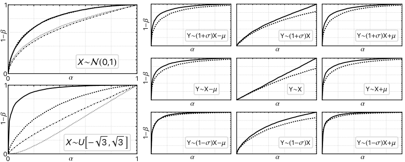
Figure S1: Left: ROC curves comparing asymptotic power of $\|S_{n,k}\|_{1,w}^{1}$ as described in Example 1 (solid line), the $F$-test (dashed), Bartlett’s test (dotted), and the Brown-Forsythe test (dot-dashed) in the context of scale shifts from $F=\mathcal{N}(0,1)$ and $F=\operatorname{Uniform\left(\left[-\sqrt{3},\sqrt{3}\right]\right)}$. Simulations used $k=10^{5},n/k=3/4$ and $\theta_{n}=\sqrt{1+n^{-1/2}}$ at $10^{5}$ Monte-Carlo iterations. Right: ROC curves comparing power of combined tests $\left(\|S_{n,k}\|_{1,w_{1}}^{1},\|S_{n,k}\|_{1,w_{2}}^{1}\right)$ (solid) and $\left(F\text{-test},t\text{-test}\right)$ (dashed) as described in Example 2. For all panels, $X\sim\mathrm{Laplace}\left(0,2^{-1/2}\right),n=18,k=24,\mu=\sigma=3/\sqrt{n}$.

Repeating the above calculations for the choice $w_{j}=w(j/k)$ where

$$\sqrt{2}w(x)=-\frac{1}{2}+\frac{d}{dt}\lim_{n\to\infty}\sqrt{n}\left[\Phi\left(\frac{\Phi^{-1}(x)}{\sqrt{1+n^{-1/2}}}\right)-t\right]=\Phi^{-1}(x)^{2}-1,$$

with $\Phi$ and $\Phi^{-}1$ the CDF and inverse CDF of a $\mathcal{N}(0,1)$ variable respectively, shows that the so obtained $\|S_{n,k}\|_{1,w}^{1}$ is consistent against $G$ as long as $\int_{0}^{1}w(x)g^{F}(x)\ \mathrm{d}x\neq 1/2$, which by symmetry of $w$ is the case under, e.g., the above-mentioned family of scale shifts if $F$ is symmetric, and provides the suitable spacing analogue of Klotz’ Gaussian score statistic [Klo62]. $\mu_{h}$ can be explicitly computed for various choices of $F$, and while the corresponding Pitman efficiencies do not mirror uniform lower bounds as were present in the context of location families (indeed, [Klo62] already showed that efficiencies can drop as low as $0.47$, conjecturing that arbitrarily small values are possible; which Proposition 4 above confirms), they behave favorably for many $F$ commonly encountered in practice. Some such efficiencies for various choices of $F$ are displayed in the left half of Figure S1 (which also includes ROC curves for two popular alternatives to the $F$-test: Bartlett’s test and the Brown-Forsythe test) and Table S1. The results broadly mirror the corresponding efficiencies for Mann-Whitney’s $U$ against the $T$-test under location shifts, and together with the fact that both the distribution exhibited in [Klo62] as well as Proposition 4 leading to efficiencies $<1$ are comparatively impractical, render $\|S_{n,k}\|_{1,w}^{1}$ with this choice of $w$ a promising, simple to use candidate for testing against scale shifts or variance differences more generally, when Gaussian or other parametric assumptions are not available (in order to calibrate the $F$-test, even asymptotically, the variance and central fourth moment of $F$ need to be known).

$F$	Gaussian	Laplace	Student’s $t$ ($\nu=5$)	Gumbel	Cauchy	$f_{Y}\in\mathcal{C}([a,b])\setminus\mathcal{C}_{0}([a,b])$
ARE	$\quad 1$	$\approx 1.23$	$\approx 2.32$	$2.59$	$\infty$	$\infty$

Table S1: Asymptotic Relative (Pitman) Efficiency of $\|S_{n,k}\|_{1,w}^{2}$ as described in Example 1 compared to $F$-test under various choices of $F$ (the distribution of $X$). The $f_{Y}\in\mathcal{C}([a,b])\setminus\mathcal{C}_{0}([a,b])$ column includes random variables $Y$ whose densities take non-zero values at at least one boundary of the support of $Y$. Either $a$ and $b$ (not necessarily both) can be finite.

Example 2 (Detecting location and scale shifts).

Given the complementary nature of Mann-Whitney’s $U$ and the spacing statistic discussed in Example 1, it is appealing to combine both tests along the lines of the discussion surrounding Proposition 3 of the main article. This is possible, since both Mann-Whitney’s $U$ and the $\|S_{n.k}\|_{1,w}$ statistic discussed in Example 1 belong to the same family of spacing statistics, allowing efficient computation and inversion of the Laplace transform and joint moments. Such combination may serve as a fully non-parametric yet powerful alternative to, e.g., the common practice of performing both $F$- and $T$-tests sequentially and reporting Bonferroni- or otherwise corrected $p$-values. Asymptotically as $n,k\to\infty$ at similar rate, $(\|S_{n,k}/n\|_{1,w_{1}},\|S_{n,k}/n\|_{1,w_{2}})$ (suitably normalized) is jointly Gaussian with covariance $\int w_{1}w_{2}$, and so explicit joint Laplace transforms or moment computations are not necessary. However, if sample sizes are small, accounting for correlations through such explicit computation may be expected to improve power over general (often conservative) $p$-value correction schemes in addition to the marginal increases of power between $\|S_{n,k}\|_{1,(\Phi^{-1}(j/k)^{2}-1)/\sqrt{2}}$ and the $F$-test, and $\|S_{n,k}\|_{1,(0,...,k)/k}$ and the $T$-test. We illustrate this on the case of comparing $(\|S_{n,k}\|_{1,(0,...,k)/k},\|S_{n,k}\|_{1,(\Phi^{-1}(j/k)^{2}-1)/\sqrt{2}})$ against the $(\text{F-Test},\text{T-Test})$ combination in the right half of Figure S1, where ROC curves for mixtures of location- and scale-shifts are plotted anchored on $X\sim\mathrm{Laplace}\left(0,1/\sqrt{2}\right)$.

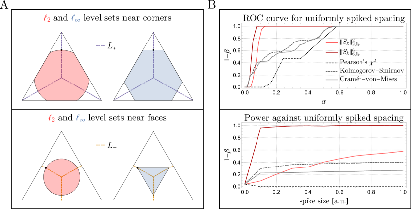
Figure S2: Analysis of spiked spacing model (described in Example 3). A. Illustration of tail probabilities on $\Delta^{2}$ in the cases of $p=2$ and $p=\infty$, and the samples (denoted by solid dots) giving rise to them. While a fixed sample near line segments in $L_{+}$ (purple, dashed lines in top panel) produces smaller sub-level sets in $\ell_{2}$ than $\ell_{\infty}$ (thereby increasing the $p$-value of said sample, which corresponds to $1$ minus the shaded area), this trend reverses for observations near line segments in $L_{-}$ (orange, dashed lines in bottom panel). B. ROC and power curves. The spiked spacing model largely concentrates around $L_{\text{corner}}$ in $\Delta^{k-1}$, with the degree of this concentration increasing with spike size. As a consequence, $p$-norms of samples generated under such alternative tend to separate more markedly for larger $p$, which in turn affords increases in power of $\|\mathchoice{\mbox{\boldmath$S$}}{\mbox{\boldmath$S$}}{\mbox{\boldmath$\scriptstyle S$}}{\mbox{\boldmath$\scriptscriptstyle S$}}_{k}\|_{p,\mathchoice{\mbox{\boldmath$1$}}{\mbox{\boldmath$1$}}{\mbox{\boldmath$\scriptstyle 1$}}{\mbox{\boldmath$\scriptscriptstyle 1$}}_{k}}^{p}$ when $p>2$. The experimental design and choices of under- and overdispersed distributions follows that of Figure $1$ in the main article.

Example 3 (Spiked spacing model and higher $p$-norms).

Due to its correspondence with the likelihood-ratio test, the choice of $p=1$ is optimal whenever data arrives in an $iid$ fashion as was the case in Examples 1 and 2. When observations exhibit correlation or are otherwise structured, larger values of $p$ may become relevant. We illustrate this phenomenon by revisiting the one-sample test in (Ref), where we sought to distinguish exponential arrival times from over- or underdispersed alternatives. We consider an alternative hypothesis $G$ of the joint distribution of $T_{1},\dots,T_{k}$ that is both over- and underdispersed in the following sense: Under $G$, arrival times are again drawn $iid$ from an underdispersed distribution $G_{1}$, with the exception of a single randomly chosen $T_{K}$ (i.e., $K\sim\mathrm{Uniform}([k])$) whose law $G_{2}$ now exhibits overdispersion. We call this overdispersed $T_{K}$ the spiked or outlier arrival time. Though the subsequent analysis is phrased in terms of this spiked spacing model, much of its reasoning pertains to similar outlier or correlation models of this kind as well.

To design a test that reliably detects this spiked spacing model, we first observe that the symmetry in $T_{1},\dots,T_{k}$ suggests little benefit of choices for $w$ other than $\mathchoice{\mbox{\boldmath$1$}}{\mbox{\boldmath$1$}}{\mbox{\boldmath$\scriptstyle 1$}}{\mbox{\boldmath$\scriptscriptstyle 1$}}_{k}$, leaving $p$ as the sole parameter to optimize. It is clear that on the level of normalized spacings, the null and alternative distributions differ only by the presence of exactly one particularly large segment, the index of which is random, and so a generalized likelihood ratio test is effectively based on the length of the longest segment. In terms of $\|\mathchoice{\mbox{\boldmath$S$}}{\mbox{\boldmath$S$}}{\mbox{\boldmath$\scriptstyle S$}}{\mbox{\boldmath$\scriptscriptstyle S$}}_{n,k}\|_{p,w}^{p}$ this corresponds to the choice $p=\infty$. To reason about intermediate values of $p$ between $1$ and $\infty$, it is useful to clarify and compare the geometry that various $\ell_{p}$ balls give rise to when intersected with $\Delta^{k-1}$: as the $2$-dimensional illustrations of Figure S2A demonstrate, the (normalized) intersection volume $V_{k}^{p}(\mathchoice{\mbox{\boldmath$s$}}{\mbox{\boldmath$s$}}{\mbox{\boldmath$\scriptstyle s$}}{\mbox{\boldmath$\scriptscriptstyle s$}})=\mu_{\Delta^{k-1}}(\|\mathchoice{\mbox{\boldmath$S$}}{\mbox{\boldmath$S$}}{\mbox{\boldmath$\scriptstyle S$}}{\mbox{\boldmath$\scriptscriptstyle S$}}_{k}\|_{p,\mathchoice{\mbox{\boldmath$1$}}{\mbox{\boldmath$1$}}{\mbox{\boldmath$\scriptstyle 1$}}{\mbox{\boldmath$\scriptscriptstyle 1$}}_{k}}^{p}\leq\|\mathchoice{\mbox{\boldmath$s$}}{\mbox{\boldmath$s$}}{\mbox{\boldmath$\scriptstyle s$}}{\mbox{\boldmath$\scriptscriptstyle s$}}\|_{p,\mathchoice{\mbox{\boldmath$1$}}{\mbox{\boldmath$1$}}{\mbox{\boldmath$\scriptstyle 1$}}{\mbox{\boldmath$\scriptscriptstyle 1$}}_{k}}^{p})$ depends on the precise location of the observation $s$. If $s$ lies exactly on any of the line segments $L_{\text{corner}}=\Big{\{}\overleftrightarrow{\hskip 2.84526pt\frac{1}{k}\mathchoice{\mbox{\boldmath$1$}}{\mbox{\boldmath$1$}}{\mbox{\boldmath$\scriptstyle 1$}}{\mbox{\boldmath$\scriptscriptstyle 1$}}_{k},\mathchoice{\mbox{\boldmath$e$}}{\mbox{\boldmath$e$}}{\mbox{\boldmath$\scriptstyle e$}}{\mbox{\boldmath$\scriptscriptstyle e$}}_{i}\hskip 2.84526pt}\Big{\}}_{i\in[k]}$, where $\mathchoice{\mbox{\boldmath$e$}}{\mbox{\boldmath$e$}}{\mbox{\boldmath$\scriptstyle e$}}{\mbox{\boldmath$\scriptscriptstyle e$}}_{i}$ is the $i^{\text{th}}$ standard basis vector, then $V_{k}^{p}(\mathchoice{\mbox{\boldmath$s$}}{\mbox{\boldmath$s$}}{\mbox{\boldmath$\scriptstyle s$}}{\mbox{\boldmath$\scriptscriptstyle s$}})\subset V_{k}^{q}(\mathchoice{\mbox{\boldmath$s$}}{\mbox{\boldmath$s$}}{\mbox{\boldmath$\scriptstyle s$}}{\mbox{\boldmath$\scriptscriptstyle s$}})$ whenever $p<q$, while $V_{k}^{p}(\mathchoice{\mbox{\boldmath$s$}}{\mbox{\boldmath$s$}}{\mbox{\boldmath$\scriptstyle s$}}{\mbox{\boldmath$\scriptscriptstyle s$}})\supset V_{k}^{q}(\mathchoice{\mbox{\boldmath$s$}}{\mbox{\boldmath$s$}}{\mbox{\boldmath$\scriptstyle s$}}{\mbox{\boldmath$\scriptscriptstyle s$}})$ in case $s$ falls precisely on any of the line segments $L_{\text{mid}}=\Big{\{}\overleftrightarrow{\hskip 2.84526pt\frac{1}{k}\mathchoice{\mbox{\boldmath$1$}}{\mbox{\boldmath$1$}}{\mbox{\boldmath$\scriptstyle 1$}}{\mbox{\boldmath$\scriptscriptstyle 1$}}_{k},\mathchoice{\mbox{\boldmath$m$}}{\mbox{\boldmath$m$}}{\mbox{\boldmath$\scriptstyle m$}}{\mbox{\boldmath$\scriptscriptstyle m$}}_{i}\hskip 2.84526pt}\Big{\}}_{i\in[k]}$, where $\mathchoice{\mbox{\boldmath$m$}}{\mbox{\boldmath$m$}}{\mbox{\boldmath$\scriptstyle m$}}{\mbox{\boldmath$\scriptscriptstyle m$}}_{i}=\frac{1}{k-1}(\mathchoice{\mbox{\boldmath$1$}}{\mbox{\boldmath$1$}}{\mbox{\boldmath$\scriptstyle 1$}}{\mbox{\boldmath$\scriptscriptstyle 1$}}_{k}-\mathchoice{\mbox{\boldmath$e$}}{\mbox{\boldmath$e$}}{\mbox{\boldmath$\scriptstyle e$}}{\mbox{\boldmath$\scriptscriptstyle e$}}_{i})$ is the midpoint of the $(k-2)$-dimensional face opposite of vertex $\mathchoice{\mbox{\boldmath$e$}}{\mbox{\boldmath$e$}}{\mbox{\boldmath$\scriptstyle e$}}{\mbox{\boldmath$\scriptscriptstyle e$}}_{i}$. Since $p$-values are $1-V_{k}^{p}(\mathchoice{\mbox{\boldmath$s$}}{\mbox{\boldmath$s$}}{\mbox{\boldmath$\scriptstyle s$}}{\mbox{\boldmath$\scriptscriptstyle s$}})$, it follows that tests based on $\|\mathchoice{\mbox{\boldmath$S$}}{\mbox{\boldmath$S$}}{\mbox{\boldmath$\scriptstyle S$}}{\mbox{\boldmath$\scriptscriptstyle S$}}_{k}\|_{\infty,\mathchoice{\mbox{\boldmath$1$}}{\mbox{\boldmath$1$}}{\mbox{\boldmath$\scriptstyle 1$}}{\mbox{\boldmath$\scriptscriptstyle 1$}}_{k}}^{\infty}$ should be most powerful in the former scenario, while $\|\mathchoice{\mbox{\boldmath$S$}}{\mbox{\boldmath$S$}}{\mbox{\boldmath$\scriptstyle S$}}{\mbox{\boldmath$\scriptscriptstyle S$}}_{k}\|_{2,\mathchoice{\mbox{\boldmath$1$}}{\mbox{\boldmath$1$}}{\mbox{\boldmath$\scriptstyle 1$}}{\mbox{\boldmath$\scriptscriptstyle 1$}}_{k}}^{2}$-based tests benefit from the latter scenario, with intermediate localizations giving rise to optimal $p^{*}$ between $2$ and $\infty$. In the spiked spacing model, the support of $G$ centers around the line segments $L_{\text{corner}}$, and so we expect choices of $p$ larger than $2$ to be profitable. Indeed, carrying out simulations as in Figure S2B reveals this to be true, with precise values of $p^{*}$ depending on the distributional details $G_{1}$ and $G_{2}$. Generally, $p^{*}$ is attained around $4$ or $5$ for modest amplitudes of the spiked $T_{K}$ and/or moderate degrees of underdispersion in the remaining arrival times, and stabilizes at $6$ for more pronounced levels of spiking and/or underdispersion. Past $p=6$, ROC and power curves tend to change only slightly.

Figure S4: Comparison of CDFs of $\|S_{n,k}\|_{1,w}$ obtained from numerical inversion (solid line) of its Laplace transform (cf. Theorem 1 in the main article) with simulations (bar chart). Six choices of $w\in\mathbb{R}^{7}$ were sampled by drawing uniform $[0,1]$ entries i.i.d. and normalizing to $\|w\|_{\infty}=1$, and corresponding draws of $\|S_{6,15}\|_{1,w}$ simulated $10,000$ times.

References

- [AB60] Abdur Rahman Ansari and Ralph A Bradley “Rank-sum tests for dispersions” In The Annals of Mathematical Statistics JSTOR, 1960, pp. 1174–1189
- [Akh20] Naum Ilích Akhiezer “The classical moment problem and some related questions in analysis” SIAM, 2020
- [AS65] Milton Abramowitz and Irene A Stegun “Handbook of Mathematical Functions: with Formulas, Graphs, and Mathematical Tables” Courier Corporation, 1965
- [Ber12] Serge Bernstein “Démonstration du théorème de Weierstrass fondée sur le calcul des probabilités” In Communications de la Société Mathématique 13.1 Imperial Kharkov University, 1912, pp. 1–2
- [Bon+14] Stefano Bonnini, Livio Corain, Marco Marozzi and Luigi Salmaso “Nonparametric hypothesis testing: rank and permutation methods with applications in R” John Wiley & Sons, 2014
- [BP70] Ake Björck and Victor Pereyra “Solution of Vandermonde systems of equations” In Mathematics of computation 24.112, 1970, pp. 893–903
- [BQM12] Jorge Bustamante, José M Quesada and Reinaldo Martínez-Cruz “Best one-sided approximation to the Heaviside and sign functions” In Journal of Approximation Theory 164.6 Elsevier, 2012, pp. 791–802
- [Bur79] Peter M Burrows “Selected percentage points of Greenwood’s statistics” In Journal of the Royal Statistical Society. Series A (General) 142.2 JSTOR, 1979, pp. 256–258
- [CJJ81] William J Conover, Mark E Johnson and Myrle M Johnson “A comparative study of tests for homogeneity of variances, with applications to the outer continental shelf bidding data” In Technometrics 23.4 Taylor & Francis, 1981, pp. 351–361
- [CO18] David Roxbee Cox and David Oakes “Analysis of survival data” ChapmanHall/CRC, 2018
- [Con+03] Knut Conradsen, Allan Aasbjerg Nielsen, Jesper Schou and Henning Skriver “A test statistic in the complex Wishart distribution and its application to change detection in polarimetric SAR data” In IEEE Transactions on Geoscience and Remote Sensing 41.1 IEEE, 2003, pp. 4–19
- [CS58] Herman Chernoff and I Richard Savage “Asymptotic normality and efficiency of certain nonparametric test statistics” In The Annals of Mathematical Statistics JSTOR, 1958, pp. 972–994
- [Cur81] Iain D Currie “Further percentage points of Greenwood’s statistic” In Journal of the Royal Statistical Society. Series A (General) 144.3 JSTOR, 1981, pp. 360–363
- [CY15] Konstantina Charmpi and Bernard Ycart “Weighted Kolmogorov Smirnov testing: an alternative for gene set enrichment analysis” In Statistical Applications in Genetics and Molecular Biology 14.3 De Gruyter, 2015, pp. 279–293
- [DAg86] Ralph B D’Agostino “Goodness-of-fit-techniques” CRC press, 1986
- [Dar53] DA Darling “On a class of problems related to the random division of an interval” In The Annals of Mathematical Statistics 24.2 JSTOR, 1953, pp. 239–253
- [Dix40] Wilfrid J Dixon “A criterion for testing the hypothesis that two samples are from the same population” In The Annals of Mathematical Statistics 11.2 JSTOR, 1940, pp. 199–204
- [Gar52] A Gardner “Greenwood’s “Problem of intervals”: An exact solution for ” In Journal of the Royal Statistical Society: Series B (Methodological) 14.1 Wiley Online Library, 1952, pp. 135–139
- [GC14] Jean Dickinson Gibbons and Subhabrata Chakraborti “Nonparametric statistical inference” CRC press, 2014
- [GG78] MH Gail and JL Gastwirth “A scale-free goodness-of-fit test for the exponential distribution based on the Gini statistic” In Journal of the Royal Statistical Society: Series B (Methodological) 40.3 Wiley Online Library, 1978, pp. 350–357
- [GJ15] Riccardo Gatto and S Rao Jammalamadaka “On two-sample tests for circular data based on spacing-frequencies” In Geometry Driven Statistics, Wiley Series in Probability and Statistics 121 Wiley, 2015, pp. 129–145
- [Gre46] Major Greenwood “The statistical study of infectious diseases” In Journal of the Royal Statistical Society 109.2 JSTOR, 1946, pp. 85–110
- [GS05] Xin Gao and Peter XK Song “Nonparametric tests for differential gene expression and interaction effects in multi-factorial microarray experiments” In BMC bioinformatics 6.1 Springer, 2005, pp. 1–13
- [HG09] Haibo He and Edwardo A Garcia “Learning from imbalanced data” In IEEE Transactions on knowledge and data engineering 21.9 Ieee, 2009, pp. 1263–1284
- [HL56] JOSEPH L Hodges Jr and Erich L Lehmann “The efficiency of some nonparametric competitors of the t-test” In The Annals of Mathematical Statistics JSTOR, 1956, pp. 324–335
- [HM05] Norbert Henze and Simos G Meintanis “Recent and classical tests for exponentiality: a partial review with comparisons” In Metrika 61.1 Springer, 2005, pp. 29–45
- [Hol72] Lars Holst “Asymptotic normality and efficiency for certain goodness-of-fit tests” In Biometrika 59.1 Oxford University Press, 1972, pp. 137–145
- [HR80] Lars Holst and JS Rao “Asymptotic Theory for Some Families of Two-Sample Nonparametric Statistics” In Sankhyā: The Indian Journal of Statistics, Series A 42 JSTOR, 1980, pp. 19–52
- [Joh+07] V John, I Angelov, AA Öncül and D Thévenin “Techniques for the reconstruction of a distribution from a finite number of its moments” In Chemical Engineering Science 62.11 Elsevier, 2007, pp. 2890–2904
- [Klo62] Jerome Klotz “Nonparametric tests for scale” In The Annals of Mathematical Statistics 33.2 Institute of Mathematical Statistics, 1962, pp. 498–512
- [Kol33] Andrey Kolmogorov “Sulla determinazione empirica di una lgge di distribuzione” In Inst. Ital. Attuari, Giorn. 4, 1933, pp. 83–91
- [Mol+20] Katie R Mollan et al. “Precise and accurate power of the rank-sum test for a continuous outcome” In Journal of biopharmaceutical statistics 30.4 Taylor & Francis, 2020, pp. 639–648
- [Moo54] Alexander M Mood “On the asymptotic efficiency of certain nonparametric two-sample tests” In The Annals of Mathematical Statistics JSTOR, 1954, pp. 514–522
- [Mor47] PAP Moran “The random division of an interval” In Supplement to the Journal of the Royal Statistical Society 9.1 JSTOR, 1947, pp. 92–98
- [Mor51] PAP Moran “The random division of an interval–Part II” In Journal of the Royal Statistical Society. Series B (Methodological) 13.1 JSTOR, 1951, pp. 147–150
- [Mor53] PAP Moran “The Random Division of an interval–Part III” In Journal of the Royal Statistical Society. Series B (Methodological) 15.1 JSTOR, 1953, pp. 77–80
- [MW47] Henry B Mann and Donald R Whitney “On a test of whether one of two random variables is stochastically larger than the other” In The Annals of Mathematical Statistics 18.1 JSTOR, 1947, pp. 50–60
- [Pal+18] PF Palamara, J Terhorst, YS Song and AL Price “High-throughput inference of pairwise coalescence times identifies signals of selection and enriched disease heritability.” In Nature Genetics 50.9, 2018, pp. 1311–1317
- [RCK07] Michael C Riley, Amanda Clare and Ross D King “Locational distribution of gene functional classes in Arabidopsis thaliana” In BMC Bioinformatics 8.1 BioMed Central, 2007, pp. 112
- [Sch19] Ulf Schepsmeier “A goodness-of-fit test for regular vine copula models” In Econometric Reviews 38.1 Taylor & Francis, 2019, pp. 25–46
- [Sch20] Konrad Schmüdgen “Ten Lectures on the Moment Problem” In arXiv preprint arXiv:2008.12698, 2020
- [SR70] J Sethuraman and JS Rao “Pitman efficiencies of tests based on spacings” In Nonparametric Techniques in Statistical Inference Cambridge University Press, 1970, pp. 405–416
- [ST60] Sidney Siegel and John W Tukey “A nonparametric sum of ranks procedure for relative spread in unpaired samples” In Journal of the American statistical association 55.291 Taylor & Francis, 1960, pp. 429–445
- [Ste81] Michael A Stephens “Further percentage points for Greenwood’s statistic” In Journal of the Royal Statistical Society. Series A (General) 144.3 JSTOR, 1981, pp. 364–366
- [Suk57] Balkrishna V Sukhatme “On certain two-sample nonparametric tests for variances” In The Annals of Mathematical Statistics 28.1 JSTOR, 1957, pp. 188–194
- [SZ00] G Schechtman and J Zinn “Concentration on the ball” In Geometric Aspects of Functional Analysis Springer, 2000, pp. 245–256
- [Tal87] Giorgio Talenti “Recovering a function from a finite number of moments” In Inverse problems 3.3 IOP Publishing, 1987, pp. 501
- [Tha10] Olivier Thas “Comparing distributions” Springer, 2010
- [Van56] BL Van der Waerden “The computation of the X-distribution” In Proc. Third Berkeley Symp. Math. Stat. Prob 1, 1956, pp. 207–208
- [Wei56] Lionel Weiss “A certain class of tests of fit” In The Annals of Mathematical Statistics 27.4 JSTOR, 1956, pp. 1165–1170
- [YLG06] Kun Yang, Jianzhong Li and Hong Gao “The impact of sample imbalance on identifying differentially expressed genes” In BMC bioinformatics 7.4 BioMed Central, 2006, pp. 1–13