Strong force fields and stabilities of the nucleon and singly heavy baryon $\Sigma_{c}$

Abstract

We investigate the strong force fields and stabilities of the nucleon and the singly heavy baryon $\Sigma_{c}$ within the framework of the chiral quark-soliton model. Having constructed the pion mean fields in the presence of the $N_{c}-1$ level quarks self-consistently, we are able to examine the gravitational form factors of $\Sigma_{c}$. We mainly focus in the present work on the stability conditions for both the nucleon and $\Sigma_{c}$ and discuss the strong force fields and their physical implications. We also present the results for the gravitational form factors and relevant observables, emphasising the difference between the nucleon and $\Sigma_{c}$.

I Introduction

While the hadron form factors of the energy-momentum tensor (EMT) have been considered as academic quantities Kobzarev:1962wt ; Pagels:1966zza for decades, the modern concept of the form factors based on the generalized parton distributions (GPDs) Mueller:1998fv ; Ji:1996ek ; Radyushkin:1996nd ; Goeke:2001tz ; Diehl:2003ny ; Belitsky:2005qn shed light on the novel understanding of the EMT form factors Teryaev:1999su ; Polyakov:2002yz . The EMT makes it possible to couple the gravity to matter, which is the reason why the EMT form factors are also called the gravitational form factors (GFFs). The hadronic matrix elements of the EMT show how the mass and spin of the hadron are distributed, and moreover provide critical information on how the corresponding hadron acquires the mechanical stability (see recent review Polyakov:2018zvc ). The conservation of the EMT yields a stability condition for a hadron. This stability condition, also known as the von Laue condition, is a nontrivial one, since it plays a role of the touchstone to disclose the validity of any theories or models of hadrons. The global stability condition constrains the 3D integral of the pressure inside a hadron should vanish. In fact, the stability conditions of hadrons are deeply rooted in chiral symmetry and its spontaneous breakdown. For example, the pressure inside the pion may hold a clue on understanding the chiral symmetry and its spontaneous breakdown Polyakov:1999gs ; Son:2014sna . Yet another form factors, which are called the $D$-term form factors $D(t)$ and are related to the spatial components of the EMT, are given in terms of the pressure and shear force, indicating that the $D$-term form factors characterize the mechanical properties of the hadrons Polyakov:2002yz . The first measurement of the nucleon GFF $D(t)$ in deeply virtual Compton scattering was reported in Ref. Burkert:2018bqq . See also Ref. Kumericki:2019ddg for discussion of subtleties in extraction of GFFs from DVCS data.

A singly heavy baryon consists of the light-quark pair and a singly heavy quark. In the limit of the infinite heavy-quark mass ($m_{Q}\to\infty$), the heavy quark spin is preserved. This leads also to the conservation of the spin of the light-quark degrees of freedom. This is often called heavy-quark spin symmetry. In this heavy-quark mass limit, the physics becomes independent of the flavor of a heavy quark, which is called heavy-quark flavor symmetry. In the nonstrange sector, we have two different representations: the isospin singlet and triplets. Since the spin state of the light-quark pair is either a spin singlet or a spin triplet, the isospin singlet that consists of a single member $\Lambda_{c}$ becomes naturally a spin singlet. On the other hand, the isospin triplets have degeneracy between the spin-$1/2$ and -$3/2$ states, which correspond to $\Sigma_{c}$ with spin 1/2 and $\Sigma_{c}^{*}$ with spin 3/2, respectively. The chromomagnetic hyperfine interaction is responsible for the removal of this degeneracy. In the present work, we will consider the GFFs of $\Sigma_{c}$ with spin 1/2. Since the light-quark pair inside $\Lambda_{c}$ is in spin-zero state and $\Sigma_{c}^{*}$ has spin 3/2, it is more instructive to consider the GFFs of $\Sigma_{c}$ in order to compare them with those of the nucleon.

The GFFs of the nucleon have been extensively investigated within various approaches Ji:1997gm ; Polyakov:2002wz ; Schweitzer:2002nm ; Goeke:2007fp ; Goeke:2007fq ; Wakamatsu:2007uc ; Cebulla:2007ei ; Jung:2013bya ; Hagler:2003jd ; Gockeler:2003jfa ; Hagler:2007xi ; Pasquini:2007xz ; Hwang:2007tb ; Abidin:2008hn ; Brodsky:2008pf ; Pasquini:2014vua ; Chakrabarti:2015lba ; Teryaev:2016edw ; Lorce:2018egm ; Shanahan:2018nnv ; Shanahan:2018pib ; Neubelt:2019sou ; Anikin:2019kwi ; Anikin:2019ufr ; Alharazin:2020yjv ; Varma:2020crx . The nucleon GFFs have been also examined within nuclear matter Kim:2012ts ; Jung:2014jja . In the present work, we want for first time to study the GFFs of the singly heavy baryon $\Sigma_{c}$ that contains a charm quark and two light quarks, emphasizing the comparison with those of the nucleon Goeke:2007fp , based on the chiral quark-soliton model ($\chi$QSM). The model was successfully extended to the description of the singly heavy baryons Yang:2016qdz , being motivated by Ref. Diakonov:2010tf . The model reproduced well the masses of the singly heavy baryons Yang:2016qdz ; Kim:2018xlc ; Kim:2019rcx . A singly heavy baryon within the $\chi$QSM is viewed as a bound state of $N_{c}-1$ level quarks. The presence of $N_{c}-1$ level quarks creates the vacuum polarization or the pion mean fields that affects self-consistently the $N_{c}-1$ level quarks. On the other hand, a heavy quark can be regarded as a mere static color source in the limit of the infinitely heavy quark mass ($m_{Q}\to\infty$). In a recent work Kim:2019rcx , it was found that the presence of $N_{c}-1$ valence quarks produces weaker pion mean fields in comparison with the case of a light baryon that consists of the $N_{c}$ valence quarks. While Refs. Yang:2016qdz ; Kim:2018xlc have assumed that this modification of the pion mean fields can be neglected and a simple strategy was taken, in which the color factor $N_{c}$ is replaced merely by $N_{c}-1$ for the valence contributions to the mass spectra of the singly heavy baryons. However, as we will describe later, the modification of the pion mean fields is crucial in computing the GFFs of a singly heavy baryon, since the stability condition is otherwise not satisfied. Therefore, we will adopt in the present work the modified pion mean fields to study the GFFs of the heavy baryon. The chiral soliton that consists of $N_{c}-1$ valence quark has either spin 0 or spin 1. The soliton with spin 0 will construct $\Lambda_{c}$ by combining itself with a heavy quark, whereas that with spin 1 will produce $\Sigma_{c}$ and $\Sigma_{c}^{*}$ together with a heavy quark. Since we are interested in comparing the GFFs of the singly heavy baryon with those of the nucleon, we will concentrate in the present work on the GFFs of $\Sigma_{c}$.

We sketch how the present work is organized: In Section II and  III, we recapitulate the general formalism for the GFFs and the stability condition for spin $1/2$ baryons briefly and explain how the GFFs of the singly heavy baryons can be computed within the framework of the $\chi$QSM. In Section IV, we present the numerical results for the GFFs of the heavy baryon $\Sigma_{c}$, emphasizing the comparison of them with those for the nucleon. We first discuss the energy densities of the $\Sigma_{c}$. Then we proceed to describe the densities of the angular momentum. Since the pressure and shear force are the essential quantities to reveal the mechanical stability of the $\Sigma_{c}$, we discuss them in detail. We also discuss the mechanical equation of states, i.e. a functional relation between the energy density and the pressure. Finally, we present the main results for the GFFs of the charmed baryon $\Sigma_{c}$. In the final Section we make summary of the present work, draw conclusions, and give outlook.

II Gravitational form factors and stability conditions

II.1 Gravitational form factors of a baryon with spin 1/2

The unpolarized GPDs $H^{q}(x,\xi,t)$ and $E^{q}(x,\xi,t)$ parametrize the matrix element of nonlocal two-quark operators on the light-cone. In the leading twist order, it can be decomposed in terms of the unpolarized GPDs as follows

$$\int\frac{d\lambda}{2\pi}e^{i\lambda x}\langle p^{\prime},\sigma^{\prime}|\overline{\psi}_{q}\left(-\frac{\lambda n}{2}\right)\not{n}\psi_{q}\left(\frac{\lambda n}{2}\right)|p,\sigma\rangle$$ (1)

$$=H^{q}(x,\xi,t)\overline{u}(p^{\prime},\sigma^{\prime})\not{n}u(p,\sigma)+E^{q}(x,\xi,t)\overline{u}(p^{\prime},\sigma^{\prime})\frac{i\sigma^{\mu\nu}n_{\mu}\Delta_{\nu}}{2M_{B}}u(p,\sigma),$$ (2)

where ${\psi}_{q}$ is the quark field with flavor $q$ on the light cone. $\sigma_{\mu\nu}$ is defined by $\sigma_{\mu\nu}=i[\gamma_{\mu},\,\gamma_{\nu}]/2$. $M_{B}$ is the corresponding mass of a baryon. $\sigma$($\sigma^{\prime}$) denotes the helicity of the initial (final) baryon state. The baryon states and Dirac spinors are normalized by $\langle p^{\prime},\sigma^{\prime}|p,\sigma\rangle=2p^{0}\delta_{\sigma^{\prime}\sigma}(2\pi)^{3}\delta(\bm{p}^{\prime}-\bm{p})$ and $\overline{u}(p)u(p)=2M_{B}\delta_{\sigma^{\prime}\sigma}$, respectively. The average of the baryon momenta and the momentum transfer are respectively defined by $P=(p+p^{\prime})/2$ and $\Delta=(p^{\prime}-p)$. $t$ designates the square of the momentum transfer, $t=\Delta^{2}$. We leave out the gauge connection between the quark operators because it becomes unity in the light-cone gauge. Note that we have suppressed the renormalization scale dependence for simplicity. The light-like vector $n$ satisfies $n^{2}=0$ and $n\cdot(p^{\prime}+p)=2$. $x$ denotes the longitudinal momentum fraction of a baryon carried by a parton whereas the $\xi$ stands for the skewedness, defined as $n\cdot\Delta=-2\xi$.

Form factors of a baryon can be defined by the Mellin moments of the GPDs with respect to $x$. The first Mellin moments of the unpolarized GPDs given in Eq. (2) yield the electromagnetic form factors of a baryon with spin 1/2 as follows:

$$\int^{1}_{-1}dx\sum_{q}H^{q}(x,\xi,t)=F_{1}(t),\ \ \ \ \ \int^{1}_{-1}dx\sum_{q}E^{q}(x,\xi,t)=F_{2}(t),$$ (3)

where $F_{1}(t)$ and $F_{2}(t)$ are the well-known Dirac and Pauli form factors of a baryon respectively. These two form factors are traditionally defined by the baryonic matrix element of the electromagnetic current

$$\langle p^{\prime},\sigma^{\prime}|\overline{\psi}_{q}(0)\gamma^{\mu}\psi_{q}(0)|p,\sigma\rangle=\overline{u}(p^{\prime},\sigma^{\prime})\left[F^{q}_{1}(t)\gamma^{\mu}+F^{q}_{2}(t)\frac{i\sigma^{\mu\nu}\Delta_{\nu}}{2M_{B}}\right]u(p,\sigma).$$ (4)

The first Mellin moments of the unpolarized GPDs for the singly heavy baryons, i.e., the electromagnetic form factors of the singly heavy baryons, were already investigated in Ref. Kim:2018nqf . The second Mellin moments of the GPDs are as equally important as the first Mellin moments, because they provide the GFFs of a baryon, which reveal mechanical properties of a baryon. Thus, the GFFs of a baryon can be defined as the second Mellin Moments as follows:

$$\int^{1}_{-1}dx\ x\ \sum_{q}H^{q}(x,\xi,t) =A^{Q}(t)+D^{Q}(t)\xi^{2},$$ (5)

$$\int^{1}_{-1}dx\ x\ \sum_{q}E^{q}(x,\xi,t) =2J^{Q}(t)-A^{Q}(t)-D^{Q}(t)\xi^{2},$$ (6)

where $J^{Q}(t)$, $A^{Q}(t)$ and $D^{Q}(t)$ are respectively defined by $J^{Q}=\sum_{q}J^{q}$, $A^{Q}=\sum_{q}A^{q}$ and $D^{Q}=\sum_{q}D^{q}$. The superscript $Q$ emphasizes the quark part of the GFFs. Note that a GPD should satisfy a polynomiality, which means that the $n$th Mellin moment of a GPD can be expressed in terms of a polynomial given by only even power of the skewedness $\xi$. The GFFs of a baryon with spin $1/2$ can be also defined by the matrix element of the EMT current

$$\langle p^{\prime},\sigma^{\prime}|\hat{T}^{a}_{\mu\nu}(0)|p,\sigma\rangle=\overline{u}(p^{\prime},\sigma^{\prime}) \bigg{[}A^{a}(t)\frac{P_{\mu}P_{\nu}}{M_{B}}+J^{a}(t)\frac{i(P_{\mu}\sigma_{\nu\rho}+P_{\nu}\sigma_{\mu\rho})\Delta^{\rho}}{2M_{B}}$$ (7)

$$+D^{a}(t)\frac{\Delta_{\mu}\Delta_{\nu}-g_{\mu\nu}\Delta^{2}}{4M_{B}}+\overline{c}^{a}(t)M_{B}g_{\mu\nu}\bigg{]}u(p,\sigma),$$ (8)

where $\hat{T}^{a=Q(G)}_{\mu\nu}$ stands for the quark (gluon) part of the QCD EMT current. $A^{a}$, $J^{a}$, and $D^{a}$ represent respectively the mass form factor, the angular momentum form factor, and the $D$-term form factor. Once these quark and gluon GFFs are separate from each other, the corresponding currents are not anymore conserved, since

$$\partial^{\mu}\hat{T}_{\mu\nu}=0,\ \ \ \ \ \hat{T}_{\mu\nu}=\hat{T}^{Q}_{\mu\nu}+\hat{T}^{g}_{\mu\nu}=\sum_{q}\hat{T}^{q}_{\mu\nu}+\hat{T}^{g}_{\mu\nu}.$$ (9)

Thus, the quark or gluon part of the GFFs should only depend on a specific scale $\mu$. However, we will suppress the scale dependence of the form factors for brevity. Actually, Eq. (9) constrains the non-conservation term $\overline{c}^{a}(t)$ to be $\overline{c}^{a}(t)=\sum_{q=Q,G}\overline{c}^{a}(t,\mu)=0$, and the total GFFs turn out to be renormalization scale invariant, i.e, $D(t)=\sum_{a}D^{a}(t,\mu)$. In fact, since the gluon degrees of freedom have been already integrated out in the present effective approach, for example, through instantons, we do not have any contributions from the gluon EMT current.

In the Breit frame, both the quark and gluon parts of the GFFs are defined by

$$T^{a}_{\mu\nu}(\bm{r},\sigma^{\prime},\sigma)=\int\frac{d^{3}\Delta}{(2\pi)^{3}2E}e^{-i\bm{\Delta}\cdot\bm{r}}\langle p^{\prime},\sigma^{\prime}|\hat{T}^{a}_{\mu\nu}(0)|p,\sigma\rangle.$$ (10)

The temporal component $T^{a}_{00}$ is related to the energy density of partons inside a baryon

$$\frac{1}{M_{B}}T^{a}_{00}(\bm{r},\sigma^{\prime},\sigma)=\int\frac{d^{3}\Delta}{(2\pi)^{3}}e^{-i\bm{\Delta}\cdot\bm{r}}\left[A^{a}(t)+\overline{c}^{a}(t)-\frac{t}{4M_{B}^{2}}\left(A^{a}(t)-2J^{a}(t)+D^{a}(t)\right)\right]\delta_{\sigma^{\prime}\sigma}.$$ (11)

By Integrating $T^{a}_{00}$ over space, one gets the mass of a spin-1/2 baryon in the rest frame

$$\int d^{3}r\sum_{a=Q,G}T^{a}_{00}(\bm{r},\sigma^{\prime},\sigma)=M_{B}A(0)=M_{B},$$ (12)

with the normalized mass form factor $A(0)=1$, where the contribution of $\overline{c}^{a}$ to $T_{00}$ is found to be zero by Eq. (9).

The mixed components $T^{a}_{0i}$ are relevant to the linear momentum and total angular momentum (spin + orbital angular momentum) densities, carried by the partons inside a baryon. According to the angular momentum operator in QCD, we define the total angular momentum distributions inside a baryon as

$$J^{a,i}_{\sigma^{\prime}\sigma}(\bm{r})=\epsilon^{ijk}r_{j}T^{a}_{0k}(\bm{r},\sigma^{\prime},\sigma)=2S^{j}_{\sigma^{\prime}\sigma}\int\frac{d^{3}\Delta}{(2\pi)^{3}}e^{-i\bm{\Delta}\cdot\bm{r}}\left[\left(J^{a}(t)+\frac{2}{3}t\frac{J^{a}(t)}{dt}\right)\delta^{ij}+\left(\Delta^{i}\Delta^{j}-\frac{1}{3}\bm{\Delta}^{2}\delta^{ij}\right)\frac{J^{a}(t)}{dt}\right].$$ (13)

Integrating $J^{a,i}_{\sigma^{\prime}\sigma}(\bm{r})$ over space gives the spin of the baryon as follows

$$\int dr^{3}\sum_{a=Q,G}J^{a,i}_{\sigma^{\prime}\sigma}(\bm{r})=2\hat{S}^{i}_{\sigma^{\prime}\sigma}J(0)=\hat{S}^{i}_{\sigma^{\prime}\sigma},$$ (14)

which is just the spin operator of a baryon.

The spatial components $T^{a}_{ij}$ charaterize mechanical properties of a baryon such as the pressure $p(r)$ and shear force $s(r)$ distributions inside a baryon. $T^{a}_{ij}$ is decomposed in terms of the irreducible tensors, so that the pressure and shear force distributions are expressed as

$$T^{a}_{ij}(\bm{r},\sigma^{\prime},\sigma)=p^{a}(r)\delta^{ij}\delta_{\sigma^{\prime}\sigma}+s^{a}(r)\bigg{(}\frac{r^{i}r^{j}}{r^{2}}-\frac{1}{3}\delta^{ij}\bigg{)}\delta_{\sigma^{\prime}\sigma}.$$ (15)

where the pressure and shear force distributions are defined as

$$p^{a}(r)=\frac{1}{6M_{B}}\frac{1}{r^{2}}\frac{1}{dr}r^{2}\frac{d}{dr}\tilde{D}^{a}(r)-M_{B}\int\frac{d^{3}\Delta}{(2\pi)^{3}}e^{-i\bm{\Delta}\cdot\bm{r}}\overline{c}^{a}(t),\ \ \ s^{a}(r)=-\frac{1}{4M_{B}}r\frac{d}{dr}\frac{1}{r}\frac{d}{dr}\tilde{D}^{a}(r),$$ (16)

with

$$\tilde{D}^{a}(r)=\int\frac{d^{3}\Delta}{(2\pi)^{3}}e^{-i\bm{\Delta}\cdot\bm{r}}D^{a}(t).$$ (17)

Equivalently, the form factor $D(t)$ can be obtained by the Fourier transform

$$D(t)=4M_{B}\int d^{3}r\frac{j_{2}(r\sqrt{-t})}{t}s(r)=12M_{B}\int d^{3}r\frac{j_{0}(r\sqrt{-t})}{2t}p(r).$$ (18)

Note that the shear force distributions of the gluon and quark separately are independent of $\overline{c}^{a}(t)$ whereas one should know it to determine the pressure distributions. In addition, we introduce a new form factor $F(t)$ that is defined by the matrix element of the trace of the total EMT operator

$$\langle p^{\prime},\sigma^{\prime}|\hat{T}^{\mu}_{\mu}(0)|p,\sigma\rangle=M_{B}F(t)\overline{u}(p^{\prime},\sigma^{\prime}){u}(p,\sigma),$$ (19)

where $F(t)$ contains all the GFFs, given by

$$F(t)=A(t)+\frac{t}{4M^{2}_{B}}\bigg{(}2J(t)-A(t)\bigg{)}-\frac{3t}{4M^{2}_{B}}D(t).$$ (20)

Then, the mean square radius $\langle r^{2}_{F}\rangle$ is obtained to be

$$\langle r^{2}_{F}\rangle=6\frac{dF(t)}{dt}\bigg{|}_{t=0}=6\left(\frac{dA(t)}{dt}-\frac{3D(t)}{4M^{2}_{B}}\right)\bigg{|}_{t=0}.$$ (21)

II.2 Stability conditions for a baryon with spin 1/2

In the static case, the spatial part of the EMT current satisfies the following conservation law

$$\partial^{i}T_{ij}=\frac{r_{j}}{r}\left[\frac{2}{3}\frac{\partial s(r)}{\partial r}+\frac{2s(r)}{r}+\frac{\partial p(r)}{\partial r}\right]=0.$$ (22)

Thus, the shear force and pressure distributions are related each other by the differential equation given in Eq. (22). By integrating Eq. (22) over space, we have one of the most important stability conditions, that is, the so-called von Laue stability condition,

$$\int^{\infty}_{0}dr\ r^{2}p(r)=0,$$ (23)

which implies that the pressure distribution has at least one node. In addition to the condition of the global stability given by Eq. (23), one can consider the conditions of the local stability Perevalova:2016dln ; Polyakov:2018rew ; Lorce:2018egm by introducing a concept of strong force field. Given the EMT densities, strong force fields can be defined as

$$dF^{i}_{(r,\theta,\phi)}=T^{ij}dS_{(r,\theta,\phi)}\bm{e}^{j}_{(r,\theta,\phi)},$$ (24)

where the normal and tangential pressure densities corresponding to $F^{i}$ are defined respectively by

$$p_{r}(r):=\frac{dF_{r}}{dS_{r}}=\frac{2}{3}s(r)+p(r),\;\;\;p_{\theta}(r):=\frac{dF_{\theta}}{dS_{\theta}}=-\frac{1}{3}s(r)+p(r),\;\;\;p_{\phi}(r):=\frac{dF_{\phi}}{dS_{\phi}}=-\frac{1}{3}s(r)+p(r),$$ (25)

where $p_{\theta}=p_{\phi}$. Using Eq. (24), Perevalova et al. Perevalova:2016dln examined a local criterion for the stability and found that at any distance $r$ the normal force should be directed outwards. This is often called the mechanical stability of a hadron. This leads to the explicit local criterion for the mechanical stability formulated as

$$p_{r}(r)>0.$$ (26)

This condition allows one to introduce the mechanical radius of a hadron

$$\langle r^{2}\rangle_{\mathrm{mech}}=\frac{\int d^{3}r~{}r^{2}p_{r}(r)}{\int d^{3}r~{}p_{r}(r)}=\frac{6D(0)}{\int^{0}_{-\infty}D(t)dt}.$$ (27)

Meanwhile, one can establish an additional stability condition by interpreting the tangential force as a two-dimensional (2D) subsystem of the whole three-dimensional (3D) system Polyakov:2018zvc . Then the 2D von Laue stability condition can be derived as

$$\int^{\infty}_{0}dr\;r\;p_{\phi}=0.$$ (28)

III Gravitational form factors of $\Sigma_{c}$ within the SU(2) chiral quark-soliton model

We will now briefly show how to compute the GFFs of the singly heavy baryon $\Sigma_{c}$ within the framework of the SU(2) $\chi$QSM. We begin from the low-energy effective QCD partition function in Euclidean space

$$Z_{\mathrm{eff}}=\int\mathcal{D}\psi\mathcal{D}\psi^{\dagger}\mathcal{D}U\mathrm{exp}\left[-\int d^{4}x\psi^{\dagger}D(U)\psi\right]=\int\mathcal{D}U\mathrm{exp}[-S_{\mathrm{eff}}],$$ (29)

where $S_{\mathrm{eff}}$ is the effective chiral action

$$S_{\mathrm{eff}}(U)=-N_{c}\mathrm{Tr\;ln}\;D(U).$$ (30)

$N_{c}$ denotes the number of colors. The Dirac operator $D(U)$ in Eq. (30) is defined by

$$D(U)=i\not{\partial}+i\hat{m}+iMU^{\gamma_{5}},$$ (31)

where $U^{\gamma_{5}}$ is called the chiral field, defined as

$$U^{\gamma_{5}}=U\frac{1+\gamma_{5}}{2}+U^{\dagger}\frac{1-\gamma_{5}}{2},$$ (32)

with

$$U=\exp\left[i{\pi^{a}\tau^{a}}\right]=\exp\left[i{P(r)\bm{n}\cdot\bm{\tau}}\right].$$ (33)

$\pi^{a}$ represents the pseudo-Nambu-Goldstone field and $\hat{m}$ is the flavor matrix of the current quark masses, written as $\hat{m}=\mathrm{diag}(m_{\mathrm{u}},\,m_{\mathrm{d}})$. We assume in the present work isospin symmetry, i.e. $m=m_{\mathrm{u}}=m_{\mathrm{d}}$. Note that we introduce the hedgehog ansatz $\pi^{a}=P(r)n^{a}$ with the profile function of the chiral soliton $P(r)$, which will be determined by solving the classical equation of motion. $\bm{n}$ is the normal unit vector along the radial direction. The Dirac Hamiltonian $h(U)$ is defined as

$$h(U)=i\gamma_{4}\gamma_{i}\partial_{i}-\gamma_{4}MU^{\gamma_{5}}-\gamma_{4}m.$$ (34)

The corresponding eigenenergies and eigenfunctions are obtained by diagonalizing the Dirac Hamiltonian as follows

$$h(U)\Phi_{n}(\bm{r})=E_{n}\Phi_{n}(\bm{r}),$$ (35)

where $E_{n}$ denote the eigenenergies of the Hamiltonian $h(U)$ and $\Phi_{n}(\bm{r})$ stand for the quark eigenfunctions. Similarly, Likewise, the free Dirac Hamiltonian ${h}_{0}$ can be defined by replacing the chiral field by the unity. The eigenvalues of $h_{0}$ are expressed as $E_{n^{0}}$. The classical soliton for singly heavy baryons consist of $N_{c}-1$ discrete level quarks bound by the pion mean field. Thus, the classical equation of motion can be derived by minimizing the energy of the classical $N_{c}-1$ soliton

$$\left.\frac{\delta}{\delta U(\bm{r})}[(N_{c}-1)E_{\mathrm{lev}}+E_{\mathrm{con}}]\right|_{U_{c}}=0.$$ (36)

where $E_{\mathrm{lev}}$ stands for the energy of the discrete bound level, and $E_{\mathrm{con}}$ is the sum of the lower Dirac continuum energies. Here, $U_{c}$ is the solution of the classical equation of motion, so that it is identified as the pion mean field. Thus, the $N_{c}-1$ soliton mass is finally derived as

$$M_{\mathrm{sol}}=(N_{c}-1)\theta(E_{\mathrm{lev}})E_{\mathrm{lev}}(U_{c})+E_{\mathrm{con}}(U_{c}).$$ (37)

The detailed calculations are presented in Ref. Kim:2019rcx . Note that as discussed in Ref. Goeke:2007fp , the stability condition is secured by the solution of the classical equation of motion.

The EMT current can be written as

$$\hat{T}_{\mu\nu}^{\mathrm{(eff)}}= -\frac{i}{4}\psi^{\dagger}(x)\left(i\gamma^{\mu}\overrightarrow{\partial}^{\nu}+i\gamma^{\nu}\overrightarrow{\partial}^{\mu}-i\gamma^{\mu}\overleftarrow{\partial}^{\nu}-i\gamma^{\nu}\overleftarrow{\partial}^{\mu}\right){\psi}(x)$$ (38)

$$-\frac{i}{4}\Psi^{\dagger}(x)\left(i\gamma^{\mu}\overrightarrow{\partial}^{\nu}+i\gamma^{\nu}\overrightarrow{\partial}^{\mu}-i\gamma^{\mu}\overleftarrow{\partial}^{\nu}-i\gamma^{\nu}\overleftarrow{\partial}^{\mu}\right){\Psi}(x),$$ (39)

where $\Psi$ denotes the heavy-quark field. Since we are interested in the GFFs of the singly heavy baryons, we need to explain how the heavy quark inside in them is treated. In the limit of the infinitely heavy-quark mass, i.s., $m_{Q}\to\infty$, the heavy quark can be regarded as a mere static color source. Thus, it does not play any important role in computing the heavy baryon GFFs for which the light quarks govern dynamics of quarks inside a singly heavy baryon.

The matrix element of the EMT current given in Eq. (39) can be computed by considering the following baryonic correlation function

$$\langle B,p^{\prime}|\hat{T}_{\mathrm{eff}}^{\mu\nu}(0)|B,p\rangle=\frac{1}{Z_{\mathrm{eff}}}\lim_{T\to\infty}\mathrm{exp}\left(ip_{4}\frac{T}{2}-ip^{\prime}_{4}\frac{T}{2}\right)\int d^{3}\bm{x}d^{3}\bm{y}\ \mathrm{exp}\left(-i\bm{p}^{\prime}\cdot\bm{y}+i\bm{p}\cdot\bm{x}\right)$$ (40)

$$\times\int\mathcal{D}\psi\mathcal{D}\psi^{\dagger}\mathcal{D}UJ_{B}(\bm{y},T/2)T_{\mu\nu}^{\mathrm{(eff)}}(0)J^{\dagger}_{B}(\bm{x},-T/2)\mathrm{exp}\left[-\int d^{4}\psi^{\dagger}D(U)\psi\right],$$ (41)

where $J_{B}$ denotes the Ioffe-type baryonic current for the $N_{c}-1$ discrete level quarks, which is expressed as

$$J_{B}(x)=\frac{1}{(N_{c}-1)!}\epsilon_{i_{1}\cdots i_{N_{c}-1}}\Gamma_{JJ_{3}TT_{3}}^{\alpha_{1}\cdots\alpha_{N_{c}-1}}\psi_{\alpha_{1}i_{1}}(x)\cdots\psi_{\alpha_{N_{c}-1}i_{N_{c}-1}}(x).$$ (42)

Here, $\alpha_{1}\cdots\alpha_{N_{c}-1}$ represent spin-flavor indices whereas $i_{1}\cdots i_{N_{c}-1}$ color indices. The matrices $\Gamma_{JJ_{3}TT_{3}}^{\alpha_{1}\cdots\alpha_{N_{c}-1}}$ are projection operators that will pick up a light-quark component of the singly heavy baryon with proper quantum numbers $JJ_{3}TT_{3}$. The creation operator $J_{B}^{\dagger}$ can be constructed in a similar way. The baryon states $|B,p\rangle$and $\langle B,p|$ are, respectively, defined by

$$|B,p\rangle =\lim_{x_{4}\to-\infty}\mathrm{exp}(-ip_{4}x_{4})\frac{1}{\sqrt{Z_{\mathrm{eff}}}}\int d^{3}x\;\mathrm{exp}(i\bm{p}\cdot\bm{x})J_{B}^{\dagger}(\bm{x},x_{4})|0\rangle,$$ (43)

$$\langle B,p| =\lim_{y_{4}\to\infty}\mathrm{exp}(-ip^{\prime}_{4}x_{4})\frac{1}{\sqrt{Z_{\mathrm{eff}}}}\int d^{3}y\;\mathrm{exp}(-i\bm{p}^{\prime}\cdot\bm{y})\langle 0|J_{B}(\bm{y},y_{4}).$$ (44)

As for a detailed formalism of the zero-mode quantization and the techniques of computing the baryonic correlation function given in Eq. (41), we refer to Ref. Christov:1995vm . The final form of the collective wave functions should be constructed by combining the $N_{c}-1$ light-quark component of the singly heavy baryon with a singly heavy quark according to a standard algebra of the angular momentum addition.

The collective baryon wave functions are finally obtained by coupling the collective $N_{c}-1$ light-quark wave functions $\psi_{J\lambda TT_{3}}(A)$ with the heavy quark spinor $\chi_{mm_{3}}$, as

$$\Psi_{\frac{1}{2}\sigma TT_{3}}(A)=\sum_{J\lambda mm_{3}}C^{\frac{1}{2}\sigma}_{J\lambda mm_{3}}\psi_{J\lambda TT_{3}}(A)\chi_{mm_{3}},$$ (45)

where $\psi_{J\lambda TT_{3}}(A)$ are expressed as

$$\psi_{J\lambda TT_{3}}(A)=(-1)^{T+T_{3}}\sqrt{2T+1}D^{J=T}_{-T_{3},\lambda}(A).$$ (46)

$\sigma$ in Eq. (45) denotes the third component of the singly heavy baryon spin. The $T$ and $T_{3}$ stand for the isospin and its third component, respectively. The $J$ and $\lambda$ represent respectively the total spin of the $N_{c}-1$ light-quark and its third component. The $m$ and $m_{3}$ designate the heavy-quark spin and its third component, respectively.

The matrix elements of the temporal, spatial, and mixed components of the EMT current are expressed in the large $N_{c}$ limit in terms of the GFFs

$$\langle p^{\prime},\sigma^{\prime}|\hat{T}^{00}_{\mathrm{eff}}|p,\sigma\rangle =2M^{2}_{B}\bigg{(}A(t)-\frac{t}{4M^{2}_{B}}D(t)\bigg{)}\delta_{\sigma^{\prime}\sigma},$$ (47)

$$\langle p^{\prime},\sigma^{\prime}|\hat{T}^{ik}_{\mathrm{eff}}|p,\sigma\rangle =\frac{1}{2}\bigg{(}\Delta^{i}\Delta^{k}-\delta^{ik}\bm{\Delta}^{2}\bigg{)}D(t)\delta_{\sigma^{\prime}\sigma},$$ (48)

$$\langle p^{\prime},\sigma^{\prime}|\hat{T}^{0k}_{\mathrm{eff}}|p,\sigma\rangle =-2iM_{B}\varepsilon^{klm}\hat{S}^{m}_{\sigma^{\prime}\sigma}\Delta^{l}J(t).$$ (49)

The matrix elements of the light-quark part of the current are obtained in the $\chi$QSM as

$$\langle p^{\prime},\lambda^{\prime}|\hat{T}^{00}_{\mathrm{eff}}|p,\lambda\rangle =2M_{B}\delta_{\lambda^{\prime}\lambda}\left((N_{c}-1)E_{\mathrm{lev}}\langle\mathrm{lev}|e^{i\bm{\Delta}\cdot\bm{x}}|\mathrm{lev}\rangle+N_{c}\sum_{n}R_{1}(E_{n},\Lambda)\langle n|e^{i\bm{\Delta}\cdot\bm{r}}|n\rangle\right),$$ (50)

$$\langle p^{\prime},\lambda^{\prime}|\hat{T}^{ik}_{\mathrm{eff}}|p,\lambda\rangle =\frac{M_{B}}{2}\delta_{\lambda^{\prime}\lambda}\left((N_{c}-1)\langle\mathrm{lev}|\{e^{i\bm{\Delta}\cdot\bm{r}},\gamma^{0}\gamma^{i}{p}^{k}\}|\mathrm{lev}\rangle+N_{c}\sum_{n}R_{2}(E_{n},\Lambda)\langle n|\{e^{i\bm{\Delta}\cdot\bm{r}},\gamma^{0}\gamma^{i}{p}^{k}\}|n\rangle\right.$$ (51)

$$\hskip 85.35826pt+(i\leftrightarrow k)\bigg{)},$$ (52)

$$\langle p^{\prime},\lambda^{\prime}|\hat{T}^{0k}_{\mathrm{eff}}|p,\lambda\rangle =\frac{M_{B}}{4I}\hat{S}^{l}_{\lambda^{\prime}\lambda}\bigg{(}(N_{c}-1)\sum_{j\neq\mathrm{lev}}\frac{\langle\mathrm{lev}|\tau^{l}|j\rangle}{E_{\mathrm{lev}}-E_{j}}\langle j|\left\{e^{i\bm{\Delta}\cdot\bm{r}},p^{k}\right\}+(E_{\mathrm{lev}}+E_{j})\gamma^{0}\gamma^{k}e^{i\bm{\Delta}\cdot\bm{r}}|\mathrm{lev}\rangle$$ (53)

$$+N_{c}\sum_{m\neq j}R_{3}(E_{m},E_{j},\Lambda)\langle m|\tau^{l}|j\rangle\langle j|\left\{e^{i\bm{\Delta}\cdot\bm{r}},p^{k}\right\}+(E_{m}+E_{j})\gamma^{0}\gamma^{k}e^{i\bm{\Delta}\cdot\bm{r}}|m\rangle\bigg{)},$$ (54)

where $R_{1}(E_{n},\Lambda)$, $R_{2}(E_{n},\Lambda)$ and $R_{3}(E_{m},E_{j},\Lambda)$ denote the regularization functions with a cutoff mass $\Lambda$ for the Dirac-continuum contributions. The corresponding expressions can be found in Appendix A. The expression for the moment of inertia $I$ can be found in Ref. Christov:1995vm . Here, we restrict ourselves to take $\sigma^{\prime}=\sigma=1/2$ without loss of any generality. Then, the expressions for the GFFs of the light-quark part are simplified to be

$$A(t)-\frac{t}{4M^{2}_{B}}D(t)=\int\frac{d\Omega_{\Delta}}{4\pi}\frac{1}{M_{B}}\left((N_{c}-1)E_{\mathrm{lev}}\langle\mathrm{lev}|e^{i\bm{\Delta}\cdot\bm{r}}|\mathrm{lev}\rangle+N_{c}\sum_{n}R_{1}(E_{n},\Lambda)\langle n|e^{i\bm{\Delta}\cdot\bm{r}}|n\rangle\right),$$ (55)

$$D(t)=\int\frac{d\Omega_{\Delta}}{4\pi}\frac{M_{B}}{t}\left((N_{c}-1)\langle\mathrm{lev}|\{e^{i\bm{\Delta}\cdot\bm{r}},\gamma^{0}\bm{\gamma}\cdot\bm{p}\}|\mathrm{lev}\rangle+N_{c}\sum_{n}R_{2}(E_{n},\Lambda)\langle n|\{e^{i\bm{\Delta}\cdot\bm{r}},\gamma^{0}\bm{\gamma}\cdot\bm{p}\}|n\rangle\right),$$ (56)

$$J(t)=\int\frac{d\Omega_{\Delta}}{4\pi}\frac{i\varepsilon^{k3m}\Delta^{k}}{2It}\bigg{(}(N_{c}-1)\sum_{j\neq\mathrm{lev}}\frac{\langle\mathrm{lev}|\tau^{3}|j\rangle}{E_{j}-E_{\mathrm{lev}}}\langle j|\left\{e^{i\bm{\Delta}\cdot\bm{r}},p^{m}\right\}+(E_{\mathrm{lev}}+E_{j})e^{i\bm{\Delta}\cdot\bm{r}}\gamma^{0}\gamma^{m}|\mathrm{lev}\rangle$$ (57)

$$\hskip 99.58464pt+N_{c}\sum_{m\neq j}R_{3}(E_{m},E_{j},\Lambda)\langle m|\tau^{3}|j\rangle\langle j|\left\{e^{i\bm{\Delta}\cdot\bm{r}},p^{m}\right\}+(E_{m}+E_{j})e^{i\bm{\Delta}\cdot\bm{x}}\gamma^{0}\gamma^{m}|m\rangle\bigg{)}.$$ (58)

When it comes to the heavy-quark part in Eq. (39) in the limit of $m_{Q}\to\infty$, the heavy quark can be regarded as a mere static color source as discussed in Ref. Hudson:2017oul . Therefore, we will adopt a naive quark model to evaluate the heavy-quark part. In this regard, one can obtain the following contributions of the singly heavy quark to the GFFs

$$A(t)=1,\ \ J(t)=\frac{1}{2},\ \ D(t)=0.$$ (59)

We want to emphasize that this heavy-quark contribution to each form factor satisfies the constraints on the form factors. That is, $A(0)$ and $J(0)$ should yield 1 and 1/2 as they should be, and the contribution to the $D$-term should vanish since the heavy quark is regarded as a free quark in the limit of $m_{Q}\to\infty$. Thus, we are able to introduce the heavy-quark mass, angular momentum and pressure distributions as the Dirac delta-function types

$$\varepsilon^{Q}(\bm{r})=m_{Q}\delta(\bm{r}),\;\;\;\rho^{\mathrm{Q}}_{J}(\bm{r})=-\frac{1}{6}\delta(\bm{r}),\;\;\;p^{\mathrm{Q}}(\bm{r})=0,$$ (60)

which are coupled with the light-quark pair. Based on these assumptions, the expressions for the GFFs are obtained as follows:

$$A(t)-\frac{t}{4M^{2}_{B}}D(t) =\frac{1}{M_{B}}\int d^{3}r\ \varepsilon(r)j_{0}(r\sqrt{-t}),$$ (61)

$$D(t) =6M_{B}\int d^{3}r\ p(r)\frac{j_{0}(r\sqrt{-t})}{t},$$ (62)

$$J(t) =3\int d^{3}r\ \rho_{J}(r)\frac{j_{1}(r\sqrt{-t})}{r\sqrt{-t}},$$ (63)

where

$$\varepsilon(r) =(N_{c}-1)E_{\mathrm{lev}}\phi^{*}_{\mathrm{lev}}(\bm{r})\phi_{\mathrm{lev}}(\bm{r})+N_{c}\sum_{n}R_{1}(E_{n},\Lambda)\phi^{*}_{n}(\bm{r})\phi_{n}(\bm{r})+m_{Q}\delta(\bm{r}),$$ (64)

$$p(r) =(N_{c}-1)\frac{1}{3}\phi^{*}_{\mathrm{lev}}(\bm{r})(\gamma^{0}\bm{\gamma}\hat{\bm{p}})\phi_{\mathrm{lev}}(\bm{r})+N_{c}\frac{1}{3}\sum_{n}R_{2}(E_{n},\Lambda)\phi^{*}_{n}(\bm{r})(\gamma^{0}\bm{\gamma}\hat{\bm{p}})\phi_{n}(\bm{r}),$$ (65)

$$\rho_{J}(r) =-(N_{c}-1)\frac{1}{6I}\sum_{j\neq\mathrm{lev}}\epsilon^{ab3}r^{a}\phi^{*}_{j}(\bm{r})\bigg{(}2\hat{p}^{b}+(E_{\mathrm{lev}}+E_{j}\gamma^{0}\gamma^{b})\bigg{)}\phi_{\mathrm{lev}}(\bm{r})\frac{\langle\mathrm{lev}|\tau^{3}|j\rangle}{E_{j}-E_{\mathrm{lev}}}$$ (66)

$$-\frac{N_{c}}{6I}\sum_{\begin{subarray}{c}n\neq j\end{subarray}}R_{3}(E_{n},E_{j},\Lambda)\epsilon^{ab3}r^{a}\phi^{*}_{j}(\bm{r})\bigg{(}2\hat{p}^{b}+(E_{n}+E_{j}\gamma^{0}\gamma^{b})\bigg{)}\phi_{n}(\bm{r})\langle n|\tau^{3}|j\rangle-\frac{1}{6}\delta(\bm{r}).$$ (67)

IV Results and discussion

Before we present the numerical results for the GFFs of the singly heavy baryons, we first explain how the parameters are fixed. The dynamical quark mass $M$ is the only free parameter in the $\chi$QSM. Its value was already determined by computing various properties of the proton, so we use the same value $M=420$ MeV. The current quark mass $m$ and cut-off mass $\Lambda$ are fixed by reproducing the experimental data on the pion mass $m_{\pi}=140$ MeV and the pion decay constant $f_{\pi}=93$ MeV. The detailed procedure for fixing these parameters can be found in Ref. Goeke:2005fs .

IV.1 Energy density

We start with examining the energy density for the mass form factor. The energy density $\varepsilon(r)$ arises from the temporal component of the EMT $T^{00}$. The integration of $\varepsilon(r)$ over space will give the mass of a singly heavy baryon as follows

$$\int d^{3}r\,\varepsilon(r)=M_{\mathrm{sol}}+m_{Q}=M_{B},$$ (68)

where $M_{B}$ stands for the mass of a singly heavy baryon. The mass form factor $A$(t) is usually normalized by Eq. (68)

$$A(0) =\frac{1}{M_{B}}\int d^{3}r\ \varepsilon(r)=1,$$ (69)

This normalization condition coincides with the constraint on the nucleon mass form factor from Ref. Goeke:2007fp . Obviously, the entire momentum of the singly heavy baryon is carried by quarks and antiquarks, since there are no gluons within the $\chi$QSM.

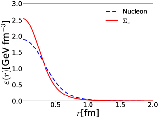
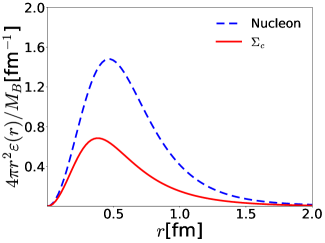
Figure 1: The comparison of the $N_{c}-1$ light-quark energy density for the singly heavy baryon $\Sigma_{c}$ with the full energy density for the nucleon. The left panel depicts the energy densities as functions of radius $r$ whereas the right panel shows the energy densities multiplied by $4\pi r^{2}$ as functions of $r$. The solid and dashed curves draw respectively $\varepsilon(r)$ for $\Sigma_{c}$ and for the nucleon.

In the left panel of Fig. 1, we compare the results for the light-quark energy density of the singly heavy baryon $\Sigma_{c}$ with that for the full energy density of the nucleon. As shown in Fig. 1, the result for $\Sigma_{c}$ is narrower than that for the nucleon. This indicates that $\Sigma_{c}$ is more compact than the nucleon. A similar tendency was already found in the case of the electromagnetic form factors of the singly heavy baryons in a previous work Kim:2018nqf where the singly heavy baryons turn out electromagnetically compact objects. Integrating the density over space yields the mass of the $N_{c}-1$ light-quark contribution to the $\Sigma_{c}$ mass, which is around $1$ GeV. Note that we find the value of the density in the center of $\Sigma_{c}$ to be $\varepsilon(0)=2.54\,\mathrm{GeV\cdot fm}^{-3}$, whereas its value of the nucleon is found to be $\varepsilon(0)=1.89~{}\mathrm{GeV\cdot fm}^{-3}$, which is smaller than that for $\Sigma_{c}$ by about 30 $\%$. On the other hand, the $\Sigma_{c}$ energy density falls off faster than that of the nucleon as $r$ increases, which results in the narrower shape of the $\Sigma_{c}$ energy density.

In the right panel of Fig. 1, we compare the weighted $\Sigma_{c}$ energy density by the usual factor $4\pi r^{2}$ with that of the nucleon. The energy density of $\Sigma_{c}$ tends to be more centered in comparison with that of the nucleon. This implies again that $\Sigma_{c}$ is more compact than the nucleon. The calculation of the radius squared will explicitly show that the $\Sigma_{c}$ is more compact than the nucleon. The radius squared of the $\Sigma_{c}$ for the mass distribution is obtained by

$$\langle r^{2}_{E}\rangle=\frac{\int d^{3}{r}\ r^{2}\varepsilon(r)}{M_{\mathrm{sol}}+m_{Q}}=\frac{1}{M_{B}}\int d^{3}{r}\ r^{2}\varepsilon(r),$$ (70)

which is identical to the derivative of the $A(t)$ form factor with respect to the momentum squared

$$\langle r^{2}_{E}\rangle=\left.\frac{6}{A(0)}\frac{\partial A(t)}{\partial t}\right|_{t=0}.$$ (71)

The results for the $A(t)$ form factor will be presented soon. The corresponding result for the mass radius squared is evaluated as follows $\langle r_{E}^{2}\rangle_{\Sigma_{c}}=0.21\,\mathrm{fm}^{2}$. On the other hand, that for the nucleon is $\langle r_{E}^{2}\rangle_{\Sigma_{c}}=0.54\,\mathrm{fm}^{2}$. Thus, we find that $\Sigma_{c}$ is indeed more compact than the nucleon.

IV.2 Angular momentum density

The density $\rho_{J}(r)$ refers to the total angular momemtum density which arises from the mixed component of the EMT current, $T^{0i}(\bm{r},\sigma^{\prime},\sigma)$, and is normalized as

$$J(0)=J_{\mathrm{sol}}(0)+J_{Q}(0) =\int d^{3}r\rho_{J}(r)=\frac{1}{2}.$$ (72)

The total angular momentum for the constituents of a baryon comes from the spin and orbital angular momenta of quarks and antiquarks, so that it should be the same as the spin of a baryon $2J(0)=1$. Concerning the heavy quark inside a singly heavy baryon, it is assumed to be static. Thus, its total angular momentum is identified as its spin. The distribution for the total angular momentum is again governed by the light-quark pair inside a singly heavy baryon.

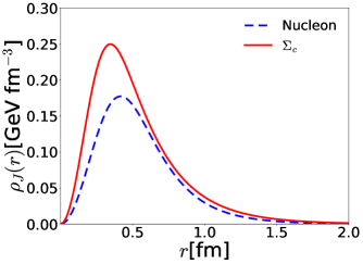
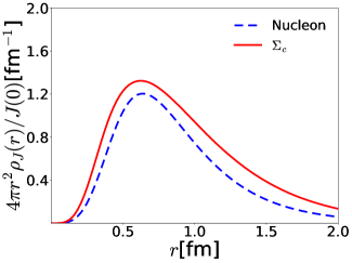
Figure 2: The comparison of the $N_{c}-1$ light-quark density for the total angular momentum of the singly heavy baryon $\Sigma_{c}$ with that for the nucleon. The left panel depicts the total angular-momentum densities as functions of radius $r$ whereas the right panel shows the total angular-momentum densities multiplied by $4\pi r^{2}$ as functions of $r$. The solid and dashed curves draw respectively $\rho_{J}(r)$ for $\Sigma_{c}$ and for the nucleon.

In the left panel of Fig. 2, we depict the numerical result for the spin distribution of $\Sigma_{c}$ in comparison with that of the nucleon. At first sight, the result seems peculiar, since the result for the spin distribution of $\Sigma_{c}$ turns out larger than that of the nucleon. However, as noted previously, the $N_{c}-1$ light-quark density corresponds to the spin 1. The spin of the $\Sigma_{c}$ baryon, which is 1/2, will be obtained by coupling that of the $N_{c}-1$ light-quark or the soliton with the singly heavy quark spin 1/2. Thus, it is natural for the spin distribution of the $N_{c}-1$ light quarks to be larger than that of the nucleon. The right panel of Fig. 2 draws the spin distribution wighted by $4\pi r^{2}$. One can make a quantitative comparison by considering the mean radius squared for the spin distribution, which is defined by

$$\langle r^{2}_{J}\rangle=\frac{\int d^{3}{r}\ r^{2}\rho_{J}(r)}{\int d^{3}{r}\ \rho_{J}(r)}=\frac{1}{J(0)}\int d^{3}{r}\ r^{2}\rho_{J}(r).$$ (73)

The results are obtained to be $\langle r^{2}_{J}\rangle_{\Sigma_{c}}=1.56\,\mathrm{fm}^{2}$ for $\Sigma_{c}$ and $\langle r^{2}_{J}\rangle_{N}=1.02\,\mathrm{fm}^{2}$ for the nucleon, respectively. This indicates that the spin distribution of $\Sigma_{c}$ is spreaded more widely than that of the nucleon. Note that in the chiral limit the angular momentum density is proportional to $r^{-4}$ at large $r$, so the radius diverges, which is very similar to the isovector radius of the nucleon Beg:1973sc ; Adkins:1983ya .

IV.3 Strong force fields and stability conditions

Using the conservation of the EMT current, we can derive the global stability condition for $\Sigma_{c}$ in Eq. (23) within the framework of the $\chi$QSM

$$\int dr\ r^{2}\ p(r) =\frac{N_{c}-1}{12\pi}\int d^{3}r\;\phi^{*}_{\mathrm{val}}(\bm{r})(\gamma^{0}\bm{\gamma}\hat{\bm{p}})\phi_{\mathrm{val}}(\bm{r})+\frac{N_{c}}{12\pi}\int d^{3}r\;\sum_{n}R_{2}(E_{n})\phi^{*}_{n}(\bm{r})(\gamma^{0}\bm{\gamma}\hat{\bm{p}})\phi_{n}(\bm{r})=0.$$ (74)

In Ref. Kim:2018xlc , the pion mean field was not newly computed but the $N_{c}$ factor was simply replaced by $N_{c}-1$ for the level parts. This brings about violation of the stability condition. To make this condition satisfied, we have to modify the pion mean field in the presence of $N_{c}-1$ light quarks, which was performed in Ref. Kim:2019rcx . In the present work, thus, we employ the improved pion mean field derived in Ref. Kim:2019rcx to compute the GFFs and the pressure density that complies with the von Laue condition. The shear force is obtained by solving the differential equation given in Eq. (22) with the boundary conditions $s(r)=0$ at $r\to 0$ and $r\to\infty$ imposed.

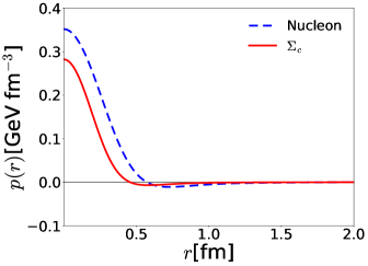
Figure 3: The comparison of the pressure distributions for $\Sigma_{c}$ with those for the nucleon. The numerical results for the pressure densities of the nucleon and $\Sigma_{c}$ are drawn as functions of radius $r$. The solid and dashed curves depict respectively those for $\Sigma_{c}$ and for the nucleon.

In Fig 3, we evaluate the pressure density for $\Sigma_{c}$ in comparison with that for the nucleon. As expected, the magnitude of the $\Sigma_{c}$ pressure density becomes smaller than that of the nucleon one, because the $N_{c}-1$ pion mean field is weaker than the $N_{c}$ pion mean field. To satisfy the global stability condition, the densities must have at least one node as shown in Fig 3. The pressures at the center of the $\Sigma_{c}$ and nucleon were estimated as $p(0)\big{|}_{\Sigma_{c}}=0.282$ GeV fm^-3 and $p(0)\big{|}_{N}=0.352$ GeV fm^-3, respectively.

We examine numerically the pressure densities of the $\Sigma_{c}$ and nucleon satisfy the following global stability conditions

$$\int dr\ r^{2}p(r) =\frac{N_{c}-1}{12\pi}\langle\widetilde{\mathrm{val}}|\gamma^{0}\bm{\gamma}\cdot\bm{p}|\widetilde{\mathrm{val}}\rangle+\frac{N_{c}}{12\pi}\sum_{n}R_{2}(E_{n},\Lambda)\langle\tilde{n}|\gamma^{0}\bm{\gamma}\cdot\bm{p}|\tilde{n}\rangle=0\;\;\mbox{ for $\Sigma_{c}$},$$ (75)

$$\int dr\ r^{2}p(r) =\frac{N_{c}}{12\pi}\langle\mathrm{val}|\gamma^{0}\bm{\gamma}\cdot\bm{p}|\mathrm{val}\rangle+\frac{N_{c}}{12\pi}\sum_{n}R_{2}(E_{n},\Lambda)\langle n|\gamma^{0}\bm{\gamma}\cdot\bm{p}|n\rangle=0\;\;\mbox{ for the nucleon},$$ (76)

where $|\widetilde{\mathrm{val}}\rangle$ and $|\tilde{n}\rangle$ emphasize the level and Dirac continuum eigenstates under the influence of the $N_{c}-1$ pion mean field.

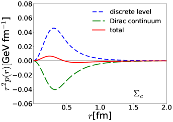
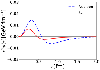
Figure 4: The left panel presents decomposition of the level and Dirac continuum contributions to the pressure. The right panel shows $r^{2}$-weighted pressures for both the light and singly heavy baryons.

In the left panel of Fig 4, we show the level and Dirac continuum contributions to the pressure density of the $\Sigma_{c}$, weighted by $r^{2}$. As in the case of the nucleon, the level quarks contribute dominantly the core part of the pressure density and are positive over the whole region of $r$, while the Dirac continuum becomes dominant in the outer part and negative. This implies that while the level quarks tend to be driven away from the center, the Dirac continuum keeps them bound in the core part. This picture is the very same as in the case of the nucleon. This gives a possible conjecture that the level quarks inside a hadron may be confined by strong vacuum fluctuations.

In the right panel of Fig 4, we compare the present results for the pressure density of $\Sigma_{c}$ with that of the nucleon. This shows that the pressure density for $\Sigma_{c}$ is overall weaker than that for the nucleon. Moreover, the comparison tells us that the size of $\Sigma_{c}$ is more compact than that of the nucleon. It can be shown clearly by introducing $r_{0}$ where the pressure density vanishes. We find $r_{0}=0.46$ fm for $\Sigma_{c}$ and $r_{0}=0.57$ fm for the nucleon. Indeed, $\Sigma_{c}$ is a more compact object than the nucleon.

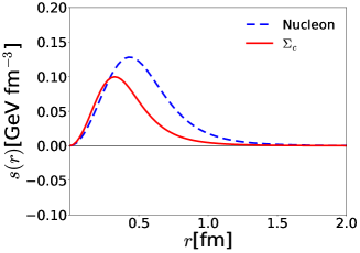
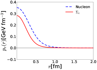
Figure 5: Comparison of the results for the shear-force density $s(r)$ and $p_{r}(r)$ of $\Sigma_{c}$ with those for the nucleon. The solid curves depict those of $\Sigma_{c}$ whereas the dashed ones draw those of the nucleon.

The left panel of Fig. 5 illustrates the result for the shear-force density of $\Sigma_{c}$ in comparison with that for the nucleon. The result for $s(r)$ of $\Sigma_{c}$ is closer to its center than that for the nucleon. The magnitude of $s(r)$ of the $\Sigma_{c}$ is smaller than that of the nucleon. The $D$-term form factor, of which the expression is given in Eq. (18), gives a clue on the signature of the shear-force density. Since $D(0)$ should be negative to comply with the stability condition, the shear-force density should be positive for all values of $r$. If we take the limit of $t\to 0$ in Eq.  (18), $D(0)$ has the following expression

$$D(0)=-\frac{4}{15}M_{B}\int d^{3}r\,r^{2}\,s(r).$$ (77)

Indeed, the results for $s(r)$ of both the nucleon and $\Sigma_{c}$ satisfy the condition $s(r)>0$. In the right panel of Fig. 5, we draw the results for $p_{r}(r)$ of the nucleon and $\Sigma_{c}$. Being similar to the case of $s(r)$, $p_{r}(r)$ is also positive for all the values of $r$. $p_{r}(r)>0$ is just a local mechanical stability condition given in Eq. (26). As shown in Fig. 5, $p_{r}(r)$ is positive definite. Note that the result for the stability density of $\Sigma_{c}$ is again weaker than that of the nucleon. This can be explained by the weaker pion mean field for singly heavy baryons. The mechanical radius is defined in terms of the stability density, which is given in Eq. (27). The numerical results for the mechanical radii of $\Sigma_{c}$ and nucleon are obtained as $\langle r^{2}\rangle^{\Sigma_{c}}_{\mathrm{mech}}=0.45$ fm² and $\langle r^{2}\rangle^{N}_{\mathrm{mech}}=0.55$ fm². This indicates that $\Sigma_{c}$ is also mechanically a more compact object than the nucleon. The size of $\Sigma_{c}$ is reduced by approximately $25~{}\%$ in comparison with that of the nucleon.

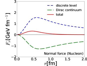
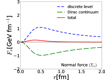
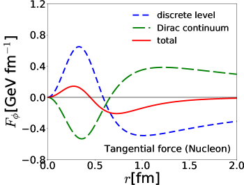
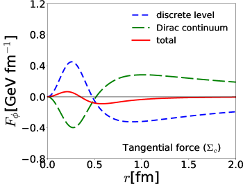
Figure 6: Results for the normal and tangential force fields in the nucleon and $\Sigma_{c}$. In the upper left panel, the results for the level and Dirac-continuum contributions to the normal force field in the nucleon is drawn in the short-dashed and long-dashed curves, respectively. In the upper right panel, those in $\Sigma_{c}$ are drawn in the same notation. In the lower left (right) panel, we depict the results for the tangential force field in the nucleon ($\Sigma_{c}$) in the same notation.

We now discuss the normal and tangential force fields defined in Eq. (24), since they shed light on how a baryon acquires its stability microscopically. In fact, the normal force field is the same as the condition of the mechanical stability except the spherical areal factor as shown in Eq. (25). We first examine the numerical results for the normal and tangential force fields as functions of $r$, which are illustrated in Fig. 6. Concerning the normal force fields in the nucleon and $\Sigma_{c}$, which are drawn in the left and right upper panels of Fig. 6 respectively, the level-quark contributions are positive definite whereas the Dirac continuum parts are negative definite. However, the magnitude of the level parts is stronger than that of the Dirac continuum parts, which leads to the fact that the normal force fields are positive definite. This implies that $F_{r}$ are directed outwards. On the other hand, the tangential force fields exhibit more complicated structures. First of all, the tangential force fields are symmetric in $\theta$ and $\phi$ as shown in Eq. (25). Thus, we do not need to distinguish $F_{\phi}$ from $F_{\theta}$. This interesting feature will be explicitly shown in three dimensional figures soon. To guarantee the stability of a baryon, the tangential force field should have at least one nodal point. The reason comes from Eq. (28) that is called the 2D von Laue stability condition. Indeed, the numerical results for $F_{\phi}$ in the nucleon and $\Sigma_{c}$ reveal one node as shown in the lower panel of Fig. 6. Interestingly, the behavior of the level-quark contributions is opposite to the Dirac continuum-quark ones, which is similar to the case of the normal force fields. This means that the direction of the tangential force field arising from the level quarks is also opposite to that from the Dirac continuum quarks. As a result, the inner part of the total tangential force fields inside both the nucleon and $\Sigma_{c}$ rotates counterclockwise from any viewpoint, whereas the outer part of $F_{\phi}$ does clockwise. We will show this feature more explicitly later.

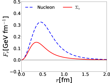
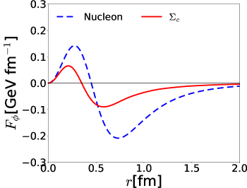
Figure 7: Comparison of the normal and tangential force fields in the nucleon with those of $\Sigma_{c}$. The solid curves depict those of $\Sigma_{c}$ whereas the dashed ones draw those of the nucleon.

In Fig. 7. we compare the numerical results for the normal and tangential force fields in $\Sigma_{c}$ with those in the nucleon. We find that both $F_{r}$ and $F_{\phi}$ in $\Sigma_{c}$ are weaker and more compact than those in the nucleon.

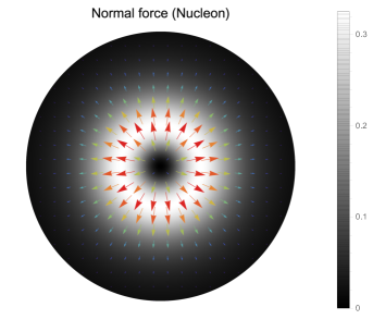
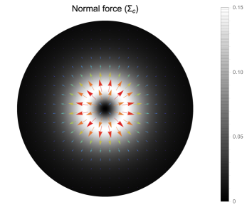
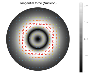
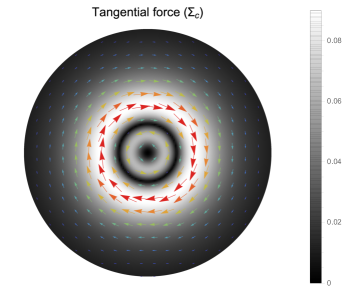
Figure 8: Visualization of the normal force fields $4\pi r^{2}T^{ij}\bm{e}^{j}_{r}$ and tangential force fields $4\pi r^{2}T^{ij}\bm{e}^{j}_{\phi}$. In the upper panel, we visualize the normal force fields in the nucleon (left) and $\Sigma_{c}$ (right), respectively. In the lower panel, we show the tangential force fields in the nucleon (left) and $\Sigma_{c}$ (right), respectively. The radius of the disc is taken to be 1.5 fm, the color legend gives the absolute value of the force fields in GeV/fm.

As discussed previously, the upper panel of Fig. 8 explicitly visualizes the fact that the normal force fields are directed outwards. On the other hand, the lower panel of Fig.  8 demonstrates how the tangential force fields rotate inside both the nucleon and $\Sigma_{c}$. The inner part of $4\pi r^{2}T^{ij}\bm{e}^{j}_{\phi}$ rotates counterclockwise, whereas the outer part of that does in the opposite direction.

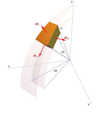
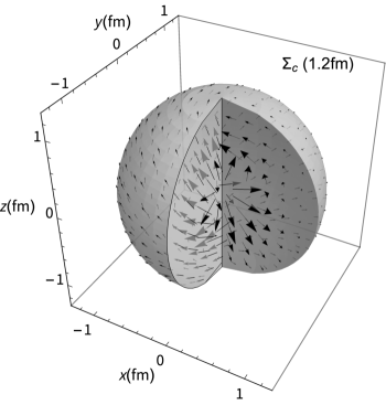
Figure 9: In the upper panel, the infinitesimal force fields $dF_{(r,\theta,\phi)}$ defined in Eq. (24) are visualized as the arrows, which will be used in the 3D visualization of the strong force fields in Fig. 10, Fig. 11 and the lower panel of Fig. 9. In the lower left and right panels, the 3D visualization of the strong force fields ($\bm{F}$) for the nucleon and $\Sigma_{c}$ are respectively illustrated, respectively.

Before illustrating the 3D visualization of the strong force fields, we first define each strong force field acting on an infinitesimal area. In the upper panel of Fig 9, the infinitesimal force fields $dF_{(r,\theta,\phi)}$ defined in Eq. (24) are visualized as the arrows, which will be used in the 3D visualization of the strong force fields. In the upper left and right panels of Fig 9, we exhibit the 3D visualization of the strong force fields ($\bm{F}$) for the nucleon and $\Sigma_{c}$, respectively.

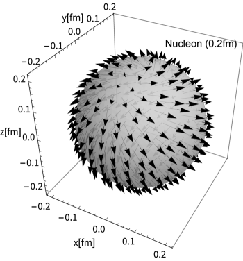
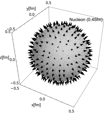
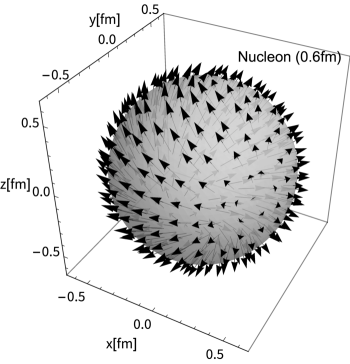
Figure 10: 3D visualization of the strong force field ($\bm{F}$) as a vector field inside a nucleon. We display the 3D force field exerting locally at each point in given shells with the distance from the center varied from $0.2$ fm, $0.45$ fm, $0.6$ fm, and $1$ fm. Note that at $0.45$ fm the tangential force field vanishes.

In Fig. 10 we illustrate how the strong force field inside a nucleon undergoes the changes as the distance from its center varies from $0.2$ fm to 1 fm. We want to emphasize that the force field acts locally on each point of a 3D surface or a shell with a given value of the distance. As shown in the upper left panel of Fig. 10, the radial component of the strong force field dominates over the tangential one. When the distance from the center reaches $0.45$ fm, the tangential force field vanishes as already shown in Fig. 6. As a result, the strong force field is directed normally outwards at $0.45$ fm as displayed in the upper right panel of Fig. 6. As $r$ further increases, however, the signature of the tangential force field is changed, which indicates that the direction of $F_{\phi}$ is reversed. This can be easily understood by comparing the upper left panel of Fig. 10 with the lower left one. When $r$ becomes larger, then $F_{\phi}$ dominates over $F_{r}$ as exhibited in the lower right panel of Fig. 10. In Fig. 11, we depict the 3D visualization of the strong force field in the case of $\Sigma_{c}$. The general behavior of the strong force field inside $\Sigma_{c}$ is very similar to the nucleon case except that the magnitude of the strong force field inside $\Sigma_{c}$ is weaker than that inside a nucleon.

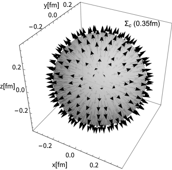
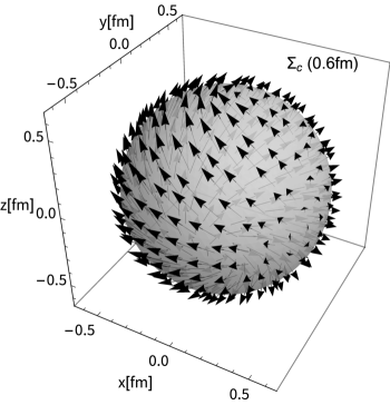
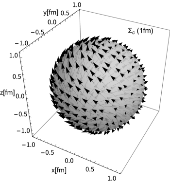
Figure 11: 3D visualization of the strong force field ($\bm{F}$) as a vector field inside $\Sigma_{c}$. We display the 3D force field exerting locally on each point in given shells with the distance from the center varied from $0.2$ fm, $0.35$ fm, $0.6$ fm, and $1$ fm. Note that at $0.35$ fm the tangential force field vanishes.

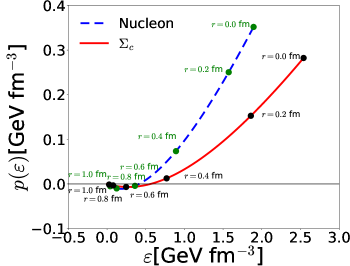
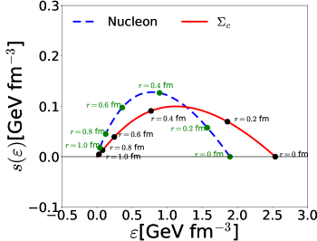
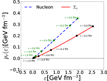
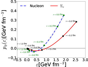
Figure 12: The results for $p(\varepsilon)$, $s(\varepsilon)$, $p_{r}(\varepsilon)$, and $p_{\phi}(\varepsilon)$. The solid curves depict those of $\Sigma_{c}$ whereas the dashed ones draw those of the nucleon.

Recently, the equation of state (EoS) inside a nucleon has been conjectured in the hope that it may give a certain clue in understanding the EoS inside compact stars Lorce:2018egm ; Polyakov:2018rew . Thus, we examine the EoS inside a nucleon and $\Sigma_{c}$. In the upper left panel of Fig. 12, we depict the pressure densities of the nucleon and $\Sigma_{c}$ as functions of the energy density, $\varepsilon$. The pressure density of the nucleon increases faster than that of $\Sigma_{c}$. This result may arise from the fact that the pion mean field for the nucleon is stronger than that for $\Sigma_{c}$. As we have discussed the results for the energy densities in Fig. 1 and those for the pressure densities in Fig. 3, the energy density of $\Sigma_{c}$ is stronger in the core part than that of the nucleon, which originates from the different pion mean fields. On the other hand, the pressure density of $\Sigma_{c}$ is overall weaker than the nucleon one by the same reason. This leads to the fact that the EoS inside the nucleon is stiffer than that inside $\Sigma_{c}$ again due to the different pion mean fields. Interestingly, $p(\varepsilon)$ of both the nucleon and $\Sigma_{c}$ become negative and are saturated, as $\varepsilon$ increases. Then $p(\varepsilon)$ starts to rise monotonically as $\varepsilon$ further increases. A similar behavior is also found in the results of $p_{\phi}(\varepsilon)$ drawn in the lower right panel of Fig. 12.

Using the EoS for the nucleon and $\Sigma_{c}$, we can recapitulate the stability conditions for the baryons. As already discussed in Fig. 1, the energy density decreases, as $r$ increases, being concentrated mainly on the inner part of the baryons. This means that the region of smaller values of $\varepsilon$ corresponds to the outer region of the baryons, in which the pressure densities are negative. As discussed previously, the contribution of the Dirac continuum is attractive whereas that of the discrete level is repulsive. One can understand this feature from the results for the EoS drawn in both the upper left panel and lower right panel of Fig. 12. It is natural that in the region of the lower energy density below approximately $\varepsilon\approx 0.5\,\mathrm{GeV\cdot fm^{-3}}$ the pressure densities should be negative. As $\varepsilon$ increases, which means that we go into the inner part of the baryons, the pressure density should become positive. As a result, the pressure density has a saturation point where $p(\varepsilon)$ starts to increase, as $\varepsilon$ increases. This observation implies that the compliance with the von Laue conditions for the stability of a baryon given in Eqs. (23) and (28) is related to the existence of the saturation point for $p(\varepsilon)$. In the upper right panel of Fig. 12, we depict the results for the shear-force densities as functions of $\varepsilon$. As discussed already in Fig. 5, $s(r)$ turns out positive for all the values of $r$. Note that the energy density is also positive definite over all the regions. As a result, $s(\varepsilon)$ turns out positive as shown in the upper right panel of Fig. 12. This indicates again that the stabilities of the nucleon and $\Sigma_{c}$ are secured. In the lower left panel of Fig. 12, we illustrate the results for $p_{r}(\varepsilon)$. Since $\varepsilon$ is positive definite over all the values of $r$, the results for $p_{r}(\varepsilon)$ imply the local stability conditions $p_{r}(r)>0$. Interestingly, they exhibit behaviors similar to the EoS for compact stars Paschalidis:2017qmb ; Weber:2004kj ; Ozel:2016oaf ; Baym:1976yu ; RikovskaStone:2006ta ; Abhishek:2018xml .

IV.4 Results for the gravitational form factors

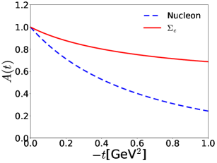
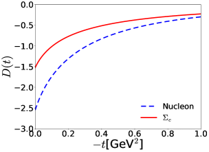
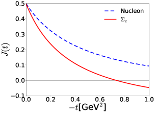
Figure 13: Results for the gravitational form factors $A(t)$, $D(t)$, and $J(t)$. The solid curves depict those of $\Sigma_{c}$ whereas the dashed ones draw those of the nucleon.

In Fig. 13 we present the numerical results for the gravitational form factors of $\Sigma_{c}$ in comparison with those of the nucleon. In the upper left panel of Fig. 13, the results for $A(t)$ show that the nucleon form factor falls off faster than that of $\Sigma_{c}$. This means that $\Sigma_{c}$ is more compact object than the nucleon. A similar feature was found in the case of the electric form factors of $\Sigma_{c}$ Kim:2018nqf . The upper right panel depicts the results for the $D$-term form factors of $\Sigma_{c}$ and the nucleon. Both the nucleon and $\Sigma_{c}$ form factors are negative, which ensures the stabilities of both the baryons. In the lower panel, we illustrate the results for the $J(t)$ form factors. In contrast to $A(t)$, the result for $J(t)$ of $\Sigma_{c}$ falls off faster than that for the nucleon. As we have mentioned previously already, the main contribution to $J(t)$ of $\Sigma_{c}$ comes from the solitonic part that has spin 1, so that the total angular-momentum density of $\Sigma_{c}$ becomes larger than the proton one, as shown in Fig. 2. This leads to the results given in the lower panel of Fig. 13. In Table 1, we list the results for various observables for the nucleon and $\Sigma_{c}$.

Table 1: Various observables for the nucleon and $\Sigma_{c}$: The energy densities at the center $\varepsilon(0)$, the mean square radii $\langle r^{2}_{E}\rangle$, $\langle r^{2}_{J}\rangle$,the pressure densities $p(0)$ at the center of the nucleon, the pressure densities $p(r_{0})=0$ at the point $r_{0}$ where they vanish, the $D$-term values $D$, the mean squared radii of the trace of the EMT, and the mechanical radii $\langle r^{2}_{\mathrm{mech}}\rangle$. We compare the results using $m_{\pi}=140$ MeV with those in the chiral limit. The heavy quark mass is taken to be $m_{c}=1.27$ GeV.

	$m_{\pi}$	$\varepsilon(0)$	$\langle r^{2}_{E}\rangle$	$\langle r^{2}_{J}\rangle$	$p(0)$	$r_{0}$	$D(0)$	$\langle r^{2}_{F}\rangle$	$\langle r^{2}_{\mathrm{mech}}\rangle$
	$[$MeV$]$	[GeV/fm3]	[fm2]	[fm2]	[GeV/fm3]	[fm]		[fm2]	[fm2]
$N$	$0$	1.66	0.65	$\infty$	0.305	0.59	-3.07	0.71	0.72
	$140$	1.89	0.54	1.02	0.352	0.57	-2.55	0.58	0.55
$\Sigma_{c}$	$0$	2.39	0.24	$\infty$	0.242	0.45	-1.79	0.28	0.64
	$140$	2.54	0.21	1.56	0.282	0.46	-1.52	0.25	0.45

V Summary and conclusions

In the present work, we aimed at investigating the stability conditions and strong force fields for the nucleon and the singly heavy baryon $\Sigma_{c}$, emphasizing the differences between them. In the chiral quark-soliton model, the pion mean field for $\Sigma_{c}$ is weaker than that for the nucleon, since the presence of the $N_{c}-1$ level quarks inside a singly heavy baryon create the pion mean field, whereas the nucleon arises as a bound state of the $N_{c}$ level quarks that are bound by the stronger $N_{c}$ pion mean field. This difference will be inherited into the results for $\Sigma_{c}$. We found that the $N_{c}-1$ pion mean fields should be evaluated self-consistently. Otherwise, the stability conditions for $\Sigma_{c}$ will be broken. Starting from the matrix elements of the energy-momentum tensor current for the nucleon and $\Sigma_{c}$, we were able to derive the four different densities: the energy densities, the total angular-momentum densities, the pressure densities, and the shear-force densities. The energy density of $\Sigma_{c}$ is narrower than that of the nucleon, which indicates that the singly heavy baryon $\Sigma_{c}$ is a more compact object than the nucleon. The total angular-momentum density of $\Sigma_{c}$ is wider and stronger than the nucleon one. This can be understood by the fact that the spin distribution of $\Sigma_{c}$ is dominated by the $N_{c}-1$ soliton that is formed as a spin 1 state whereas the spin distribution of the nucleon arises from the $N_{c}$ soliton with spin 1/2. We found that the present results for the pressure and shear-force densities satisfy both the global and local stability conditions. As already shown in the previous work in the chiral quark-soliton model Goeke:2007fp , the global stability condition for the nucleon is also secured by the balance between the leavel-quark and Dirac-continuum contributions. The results for $\Sigma_{c}$ also satisfy the stability conditions in the same manner. The shear-force densities turned out positive definite over all the values of the distance from the center of the baryons.

The strong force fields are defined in terms of the pressure and shear-force densities, which are exerted on the shell of $\Sigma_{c}$ and the nucleon, given a distance from the center of the baryons. The strong force fields can be decomposed into the normal and tangential components, which are expressed by the normal and tangential densities. These two densities are written in terms of the pressure and shear-force ones. In particular, the positivity of the normal pressure density is identified as the local stability condition. The results for the normal pressure densities of the nucleon and $\Sigma_{c}$ fulfill the local stability condition for them. The tangential components of the strong force fields for the nucleon and $\Sigma_{c}$ have at least one nodal point as in the case of the pressure densities. This indicates that the tangential force fields should change the direction. Thus, they swirl counterclockwise in the inner parts of both the nucleon and $\Sigma_{c}$, whereas they circulate around oppositely in the outer regions of the nucleon and $\Sigma_{c}$. We also examined the equations of state with the conjecture that the results for them may shed light on the inner structure of compact stars.

Finally, we presented the results for the gravitational form factors of the nucleon and $\Sigma_{c}$. The mass form factor of the $\Sigma_{c}$ falls off slower than that of the nucleon, which implies that $\Sigma_{c}$ is a more compact object than the nucleon. As expected from the discussion of the stability conditions, the $D$-term form factors of both the nucleon and $\Sigma_{c}$ turn out to be negative. The total angular-momentum form factor of $\Sigma_{c}$ falls off faster than that for the nucleon in contrast to the case of the energy form factors. The reason comes from the fact that the main contribution to the total angular-momentum form factor of $\Sigma_{c}$ is governed by the solitonic part with spin 1.

The present work can be extended to the grativational form factors of the baryon sextet and decuplet. To do that, we need to consider explicitly the strange-quark contributions and to see how the strange quarks come into play in understanding the stabilities of the baryons with spin 3/2. The corresponding investigations are under way.

Appendix A Regularization functions

The proper-time regularization functions used in Eq. (54), Eq. (58) and Eq. (67) are defined by

$$R_{1}(E_{n},\Lambda) =\frac{1}{4\sqrt{\pi}}\int^{\infty}_{\Lambda^{-2}}\frac{du}{u^{3/2}}e^{-uE^{2}_{n}},$$ (78)

$$R_{2}(E_{n},\Lambda) =\frac{1}{4\sqrt{\pi}}\int^{\infty}_{\Lambda^{-2}}\frac{du}{u^{1/2}}E_{n}e^{-uE^{2}_{n}},$$ (79)

$$R_{3}(E_{n},E_{m},\Lambda) =\frac{1}{4\sqrt{\pi}}\int^{\infty}_{\Lambda^{-2}}\frac{du}{u^{1/2}}\left(\frac{e^{-uE^{2}_{n}}-e^{-uE^{2}_{m}}}{u^{3/2}(E^{2}_{m}-E^{2}_{n})}-\frac{E_{n}e^{-uE^{2}_{n}}-E_{m}e^{-uE^{2}_{m}}}{u^{1/2}(E_{m}+E_{n})}\right).$$ (80)

References

- (1) I. Kobzarev and L. Okun, Zh. Eksp. Teor. Fiz. 43 (1962), 1904-1909
- (2) H. Pagels, Phys. Rev. 144 (1966), 1250-1260
- (3) D. Müller, D. Robaschik, B. Geyer, F.-M. Dittes and J. Hořejši, Fortsch. Phys. 42, 101 (1994).
- (4) X. D. Ji, Phys. Rev. Lett. 78, 610 (1997).
- (5) A. V. Radyushkin, Phys. Lett. B 380, 417 (1996).
- (6) K. Goeke, M. V. Polyakov and M. Vanderhaeghen, Prog. Part. Nucl. Phys. 47, 401 (2001).
- (7) M. Diehl, Phys. Rept. 388, 41 (2003).
- (8) A. Belitsky and A. Radyushkin, Phys. Rept. 418 (2005), 1-387 [arXiv:hep-ph/0504030 [hep-ph]].
- (9) O. V. Teryaev, [arXiv:hep-ph/9904376 [hep-ph]].
- (10) M. V. Polyakov, Phys. Lett. B 555, 57 (2003) [hep-ph/0210165].
- (11) V. D. Burkert, L. Elouadrhiri and F. X. Girod, Nature 557 (2018) no.7705, 396-399
- (12) K. Kumericki, Nature 570 (2019) no.7759, E1-E2
- (13) M. V. Polyakov and P. Schweitzer, Int. J. Mod. Phys. A 33 (2018) no.26, 1830025 [arXiv:1805.06596 [hep-ph]].
- (14) M. V. Polyakov and C. Weiss, Phys. Rev. D 60 (1999), 114017 [arXiv:hep-ph/9902451 [hep-ph]].
- (15) H.-D. Son and H-Ch. Kim, Phys. Rev. D 90 (2014) no.11, 111901 [arXiv:1410.1420 [hep-ph]].
- (16) X. Ji, W. Melnitchouk and X. Song, Phys. Rev. D 56 (1997), 5511-5523 [arXiv:hep-ph/9702379 [hep-ph]].
- (17) M. V. Polyakov and A. G. Shuvaev, “On’dual’ parametrizations of generalized parton distributions,” [arXiv:hep-ph/0207153 [hep-ph]].
- (18) P. Schweitzer, S. Boffi and M. Radici, Phys. Rev. D 66 (2002), 114004 [arXiv:hep-ph/0207230 [hep-ph]].
- (19) K. Goeke, J. Grabis, J. Ossmann, M. Polyakov, P. Schweitzer, A. Silva and D. Urbano, Phys. Rev. D 75 (2007), 094021 [arXiv:hep-ph/0702030 [hep-ph]].
- (20) K. Goeke, J. Grabis, J. Ossmann, P. Schweitzer, A. Silva and D. Urbano, Phys. Rev. C 75, 055207 (2007) [hep-ph/0702031 [HEP-PH]].
- (21) M. Wakamatsu, Phys. Lett. B 648 (2007) 181-185 [arXiv:hep-ph/0701057 [hep-ph]].
- (22) C. Cebulla, K. Goeke, J. Ossmann and P. Schweitzer, Nucl. Phys. A 794 (2007), 87-114 [arXiv:hep-ph/0703025 [hep-ph]].
- (23) J.-H. Jung, U. Yakhshiev and H.-Ch. Kim, J. Phys. G 41 (2014), 055107 [arXiv:1310.8064 [hep-ph]].
- (24) P. Hägler et al. [LHPC and SESAM Collaborations], Phys. Rev. D 68, 034505 (2003) [hep-lat/0304018].
- (25) M. Göckeler et al. [QCDSF Collaboration], Phys. Rev. Lett. 92, 042002 (2004) [hep-ph/0304249].
- (26) P. Hagler et al. [LHPC Collaboration], Phys. Rev. D 77 (2008) 094502 [arXiv:0705.4295 [hep-lat]].
- (27) B. Pasquini and S. Boffi, Phys. Lett. B 653 (2007) 23 [arXiv:0705.4345 [hep-ph]].
- (28) D. S. Hwang and D. Mueller, Phys. Lett. B 660 (2008) 350 [arXiv:0710.1567 [hep-ph]].
- (29) Z. Abidin and C. E. Carlson, Phys. Rev. D 77 (2008) 115021 [arXiv:0804.0214 [hep-ph]].
- (30) S. J. Brodsky and G. F. de Teramond, Phys. Rev. D 78 (2008) 025032 [arXiv:0804.0452 [hep-ph]].
- (31) B. Pasquini, M. V. Polyakov and M. Vanderhaeghen, Phys. Lett. B 739 (2014) 133 [arXiv:1407.5960 [hep-ph]].
- (32) D. Chakrabarti, C. Mondal and A. Mukherjee, Phys. Rev. D 91 (2015) 114026 [arXiv:1505.02013 [hep-ph]].
- (33) O. V. Teryaev, Front. Phys. (Beijing) 11 (2016) no.5, 111207
- (34) C. Lorce, H. Moutarde and A. P. Trawinski Eur. Phys. J. C 79 (2019) no.1, 89 [arXiv:1810.09837 [hep-ph]].
- (35) P. E. Shanahan and W. Detmold, Phys. Rev. Lett. 122 (2019) no.7, 072003 [arXiv:1810.07589 [nucl-th]].
- (36) P. E. Shanahan and W. Detmold, Phys. Rev. D 99 (2019) no.1, 014511 [arXiv:1810.04626 [hep-lat]].
- (37) M. J. Neubelt, A. Sampino, J. Hudson, K. Tezgin and P. Schweitzer, Phys. Rev. D 101 (2020) 034013 [arXiv:1911.08906 [hep-ph]].
- (38) I. V. Anikin, Phys. Rev. D 99 (2019) no.9, 094026 [arXiv:1902.00094 [hep-ph]].
- (39) I. V. Anikin, Particles 2 (2019) no.3, 357-364 [arXiv:1906.11522 [hep-ph]].
- (40) H. Alharazin, D. Djukanovic, J. Gegelia and M. V. Polyakov, [arXiv:2006.05890 [hep-ph]].
- (41) M. Varma and P. Schweitzer, [arXiv:2006.06602 [hep-ph]].
- (42) H.-Ch. Kim, P. Schweitzer and U. Yakhshiev, Phys. Lett. B 718 (2012) 625-631 [arXiv:1205.5228 [hep-ph]].
- (43) J.-H. Jung, U. Yakhshiev, H.-Ch. Kim and P. Schweitzer, Phys. Rev. D 89 (2014) 114021 [arXiv:1402.0161 [hep-ph]].
- (44) G. S. Yang, H.-Ch. Kim, M. V. Polyakov and M. Praszałowicz, Phys. Rev. D 94 (2016) 071502 [arXiv:1607.07089 [hep-ph]].
- (45) D. Diakonov, arXiv:1003.2157 [hep-ph].
- (46) J.-Y. Kim, H.-Ch. Kim and G. S. Yang, Phys. Rev. D 98 (2018) 054004.
- (47) J.-Y. Kim and H.-Ch. Kim, PTEP 2020 (2020) no.4, 043D03 [arXiv:1909.00123 [hep-ph]].
- (48) J.-Y. Kim and H.-Ch. Kim, Phys. Rev. D 97, no. 11, 114009 (2018) [arXiv:1803.04069 [hep-ph]].
- (49) I. A. Perevalova, M. V. Polyakov and P. Schweitzer, Phys. Rev. D 94, no. 5, 054024 (2016) [arXiv:1607.07008 [hep-ph]].
- (50) M. V. Polyakov and P. Schweitzer, PoS SPIN 2018, 066 (2019) [arXiv:1812.06143 [hep-ph]].
- (51) C. V. Christov, A. Blotz, H.-Ch. Kim, P. Pobylitsa, T. Watabe, T. Meissner, E. Ruiz Arriola and K. Goeke, Prog. Part. Nucl. Phys. 37, 91 (1996).
- (52) J. Hudson and P. Schweitzer, Phys. Rev. D 97, no.5, 056003 (2018) [arXiv:1712.05317 [hep-ph]].
- (53) K. Goeke, J. Ossmann, P. Schweitzer and A. Silva, Eur. Phys. J. A 27, 77 (2006) [hep-lat/0505010].
- (54) M. A. B. Bég and A. Zepeda, Phys. Rev. D 6 (1972) 2912.
- (55) G. S. Adkins, C. R. Nappi and E. Witten, Nucl. Phys. B 228 (1983) 552.
- (56) V. Paschalidis, K. Yagi, D. Alvarez-Castillo, D. B. Blaschke and A. Sedrakian, Phys. Rev. D 97 (2018) 084038 [arXiv:1712.00451 [astro-ph.HE]].
- (57) F. Weber, Prog. Part. Nucl. Phys. 54 (2005), 193-288 [arXiv:astro-ph/0407155 [astro-ph]].
- (58) F. Özel and P. Freire, Ann. Rev. Astron. Astrophys. 54 (2016), 401-440 [arXiv:1603.02698 [astro-ph.HE]].
- (59) G. Baym and S. A. Chin, Phys. Lett. 62B (1976) 241.
- (60) J. Rikovska-Stone, P. A. M. Guichon, H. H. Matevosyan and A. W. Thomas, Nucl. Phys. A 792 (2007) 341 [nucl-th/0611030].
- (61) A. Abhishek and H. Mishra, Phys. Rev. D 99 (2019) no.5, 054016 [arXiv:1810.09276 [hep-ph]].