Orthogonalized SGD and Nested Architectures for Anytime Neural Networks

Abstract

We propose a novel variant of SGD customized for training network architectures that support anytime behavior: such networks produce a series of increasingly accurate outputs over time. Efficient architectural designs for these networks focus on re-using internal state; subnetworks must produce representations relevant for both immediate prediction as well as refinement by subsequent network stages. We consider traditional branched networks as well as a new class of recursively nested networks. Our new optimizer, Orthogonalized SGD, dynamically re-balances task-specific gradients when training a multitask network. In the context of anytime architectures, this optimizer projects gradients from later outputs onto a parameter subspace that does not interfere with those from earlier outputs. Experiments demonstrate that training with Orthogonalized SGD significantly improves generalization accuracy of anytime networks.

1 Introduction

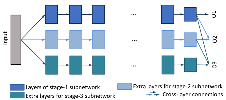
Figure 1: Ensemble of three different deep neural networks.

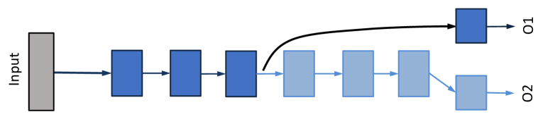
Figure 2: Cascade with branching outputs. Networks are nested in depth, sharing a common trunk to which output branches attach. (Box colors indicate in which inference stage a layer is introduced, as in Figure 3).

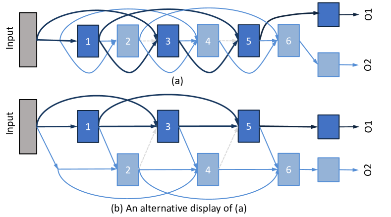
Figure 3: Our interlaced depth-wise nesting design for anytime networks. Recursive interlacing produces additional nested stages (beyond the two diagrammed here), each time doubling overall network depth. This design allows more synergistic coordination between networks than the branched topology shown in Figure 3.

The accuracy of deep neural networks is affected by both their architecture and overall size. On one hand, improving architecture, via either principled design (Simonyan & Zisserman, 2015; Szegedy et al., 2015; He et al., 2016) or automated search (Zoph & Le, 2017; Pham et al., 2018; Xie et al., 2019), has been a major research focus; on the other, fixing a particular architectural motif, increasing network size (i.e. width and depth) provides a path to further improvement in accuracy—a trend prevalent among dominant architectures in major application areas, including computer vision (He et al., 2016; Zagoruyko & Komodakis, 2016) and natural language processing (Devlin et al., 2018). The higher accuracy of larger networks comes at the cost of increased compute requirements and longer inference latency. Real applications may be deployed on hardware (e.g. mobile) and in use cases (e.g. interactive, real-time) that cap permissible network designs in both compute and latency.

Network compression techniques (Bucilua et al., 2006; Han et al., 2016) can provide means of meeting some types of known, fixed resource constraints. The pruning paradigm (Han et al., 2016) removes parameters throughout a network, reducing memory and FLOP requirements, while distillation approaches (Han et al., 2016; Hinton et al., 2015) can also shrink network depth and thereby reduce latency. However, none of these techniques handle dynamic run-time environments, where applications may need to adjust accuracy-compute-latency trade-offs in real-time. For example, interactivity requirements may present dynamically changing latency deadlines for predictions (Dollar et al., 2011; Fowers et al., 2018); concurrently running applications can compete for computation resources and power budget (Hoffmann & Maggio, 2014) in unpredictable ways (Zhuravlev et al., 2010). These environmental factors could change while inference is executing (Lin et al., 2018), defeating attempts to statically schedule around them.

Anytime predictors (Zilberstein, 1996) are a promising approach to generating accurate inference results under dynamic latency and resource constraints. They produce complete outputs at multiple intermediate stages, ameliorating penalties associated with failure to complete an inference process. If interrupted, an intermediate prediction—though less accurate—substitutes for the originally desired output, thereby preventing catastrophic failure. General approaches to building anytime predictors include ensembling (Dietterich, 2000) multiple independent predictors (Figure 3) and reorganizing a standard prediction pipeline into a cascade (Zilberstein, 1996) (Figure 3), both of which can be exploited to build anytime variants of deep networks (Wang et al., 2019; Lee & Shin, 2018; Huang et al., 2017a; McGill & Perona, 2017; Teerapittayanon et al., 2016).

Unfortunately, anytime flexibility is not free. Existing anytime network design and training procedures sacrifice considerable accuracy and/or require significant extra computation to produce intermediate predictions. We reduce these costs by introducing synergistic innovations across both anytime network architectures and training procedures.

On the architectural aspect, we propose new structures for anytime neural networks according to a principle of maximizing the potential for re-use of intermediate state between successive stages. A small network should not only produce a quick output, but should also produce internal representations that serve as valuable input to larger networks in subsequent stages. We thus design architectures so that connections between subnetworks in different stages are aligned: they directly link corresponding pairs of layers across stages, so as to allow subsequent subnetworks to refine previously computed internal representations.

Maximizing the potential for cooperative refinement leads to a class of recursively-nested anytime networks, in which later subnetworks fully contain earlier ones, while growing in width, depth, or a combination thereof. Compared to prior work (Teerapittayanon et al., 2016; Huang et al., 2017a) using branched cascade architectures (Figure 3), our alignment principle suggests a depth-nesting approach based on interlacing subnetwork layers (Figure 3). Conveniently, a recently proposed improvement (Zhu et al., 2018) to residual networks (He et al., 2016), though not an anytime design itself, is amenable to adaptation into an interlaced, depth-nested form; we defer details to Section 3.

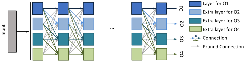
Figure 4: Width-wise nesting of deep networks. Compared to a standard network, each layer is sliced into multiple layers (colored blocks, stacked vertically). Each successive subnetwork includes another set of layer slices across the entire depth of the network.

Nesting networks width-wise is more straightforward (Figure 4) and, unlike depth-nesting, previously-explored solutions (Lee & Shin, 2018) agree with our alignment principle. We do, however, propose an improvement to width-nesting: subsequent stages should grow exponentially, rather than linearly, in width. This same scaling strategy applies to our novel depth-nesting approach. Experiments in Section 5 demonstrate the efficacy of interlaced depth-nesting, as well as how exponential scaling of subnetwork size in width- and/or depth-nested scenarios yields anytime networks that cover a broad accuracy-compute trade-off curve.

Complementary to our architectural innovations, we propose a novel optimizer, Orthogonalized SGD (OSGD), for training anytime neural networks. Motivating OSGD is a view of anytime networks as a special-case of multitask networks, combined with a desire to facilitate synergy between those tasks. In addition to synergistic architectures, we want another type of synergy: synergy in the optimization dynamics when training those multitask architectures.

Here, the multiple tasks are different versions of the same task, restricted to use only parameters within a particular subnetwork. The partially-shared structure of anytime networks, present in classical cascades and our nested topologies, means that tasks may compete for use of shared parameters. At the same time, the highly-related nature of the tasks means that they may also act as regularizers for one another. OSGD provides a methodology for re-balancing task interactions as they simultaneously pull on network parameters over the course of training. Section 4 presents the technical details of our re-balancing approach, which operates on a set of task-specific parameter gradients.

While OSGD is general, with potential application to any multitask training scenario, we restrict focus to anytime networks. We observe dramatic improvements in generalization accuracy when training anytime networks with OSGD—a result that holds across the full spectrum of anytime network architectures. Training our fully-nested anytime networks with Orthogonalized SGD sufficiently improves accuracy to the point of making such networks competitive with standard designs lacking anytime flexibility. Together, the techniques we develop here provide a pathway toward endowing deep neural networks with anytime flexibility at minimal overhead cost; as a consequence, perhaps anytime designs should become the new default architectural schema.

2 Related Work

2.1 Dynamic Inference and Anytime Deep Networks

Anytime algorithms have a well-established history, with computational strategies applicable to many learning techniques (Zilberstein, 1996). Classic approaches include anytime decision trees using ensembles or boosting (Grubb & Bagnell, 2012; Viola & Jones, 2004; Xu et al., 2013, 2012). Past focus includes domains such as visual perception (Viola & Jones, 2004), which is now dominated by methods based on deep neural networks. Adapting anytime techniques to modern deep networks is of particular importance given their computational demands and their potential use in real-time safety-critical systems, such as autonomous vehicles (Huval et al., 2015; Chen et al., 2015; Dosovitskiy et al., 2017; Teichmann et al., 2018).

Complementary to recent methods for statically reducing neural network model size (Han et al., 2016; Hinton et al., 2015; Iandola et al., 2016; Rastegari et al., 2016; Howard et al., 2017), another branch of investigation has focused on reducing inference time in a dynamic, input-dependent manner (Figurnov et al., 2017; McGill & Perona, 2017; Veit & Belongie, 2018; Wu et al., 2018; Ren et al., 2018). These adaptive inference methods skip execution of parts of a network, based on an estimate of relevance computed for each input; their goal is to minimize computation required for accurate prediction on a per-example basis. Here, the inference procedure changes dynamically in response a network’s input data. However, these approaches do not provide any mechanism for responding to environmental conditions that might introduce transient resource constraints to the system.

Anytime methods, in contrast, do provide means of addressing such environmental variability. Specifically, they aim to introduce a degree of robustness to dynamic environmental effects, at the possible cost of moderately increased computation. For example, a recent anytime design by Wang et al. (2019) develops a prediction pipeline specifically for stereo depth estimation, outputting images with increasing spatial resolution, an approach that may not generalize to other domains. Recent generic anytime approaches include several cascade designs (Larsson et al., 2017; Teerapittayanon et al., 2016; Huang et al., 2017a; Hu et al., 2019), which grow subnetworks by depth, and a recent proposal (Lee & Shin, 2018) that grows by width, as discussed in Section 1. We compare our anytime designs with them both conceptually and experimentally; Sections 3 and 5 provide details.

2.2 Multitask Training

Caruana (1997) suggests that multitask training can improve generalization performance of machine learning systems. Recent advances highlight the ability of learned neural representations to transfer between related tasks within particular domains, including vision (Donahue et al., 2014) and natural language processing (Devlin et al., 2018). Fine-tuning previously trained networks for new tasks has become a standard mode of operation.

Multitask learning has successes in multiple areas, including vision (Kokkinos, 2017; Eigen & Fergus, 2015; Teichmann et al., 2018), natural language processing (Collobert & Weston, 2008; Hashimoto et al., 2016; Søgaard & Goldberg, 2016), speech (Seltzer & Droppo, 2013; Wu et al., 2015), and cross-domain representations (Bilen & Vedaldi, 2017). However, training such systems is a non-trivial problem. Long & Wang (2015); Misra et al. (2016) use clustering methods; Yang & Hospedales (2017) separate general and task-specific features; Kokkinos (2017); Larsson (2017) train all tasks with the same base network and a few task-specific layers; Kendall et al. (2018); Hu et al. (2019) build joint losses with adaptive weights.

Notably, Kokkinos (2017) finds it difficult to train a single convolutional network for multimodal visual perception to the point of matching the accuracy of more specialized task-specific networks. This observation runs contrary to the expectation that visual perception tasks should be highly related to one another, sparking interest in developing methods to quantify task interdependence (Zamir et al., 2018).

Similar in spirit to our approach, prior works have targeted changes to optimizers to improve multitask network training. This includes NormSGD (Larsson, 2017), which computes a parameter gradient per task, in separate backpropagation passes. These gradient vectors are then normalized before summation, ensuring that each task exerts equal influence on network parameters at every training iteration. Kendall et al. (2018) take another approach to dynamically balancing task influence, allowing some slack in relative task importance, provided it is justified by outsized gains in accuracy across the task spectrum as a whole. Our OSGD optimizer, like NormSGD, attempts to dynamically re-balance task interactions. However, OSGD addresses a different kind of interaction, making it composable with most existing optimizers; we also test an Orthogonalized NormSGD variant.

2.3 Gradient Orthogonality

Directly related to our method for reasoning about task interactions is the work of Farajtabar et al. (2020). Like Farajtabar et al. (2020), we view task interactions through the lens of their parameter gradient vectors. That is, for a multitask network, comparing per-task gradient vectors (computed via separate backpropagation passes) tells us about task similarity: aligned gradients indicate synergy between tasks, while opposing gradient directions suggest competition. Orthogonal vectors suggest the tasks do not interfere with one another; they each pull on a parameter subspace about which the other is agnostic.

Farajtabar et al. (2020) translate these intuitions into an algorithmic approach for fine-turning that resists catastrophic forgetting. Their goal is to train an existing neural network to perform an additional task while ensuring that it retains the ability to accurately perform a task it has previously learned. Farajtabar et al. (2020) model the parameter subspace of the original task using a collection of parameter gradient vectors for a sample of that task’s training examples. When training a new task, they project its gradients onto the subspace orthogonal to that spanned by this collection. Even if using only a few hundred samples, this projection step can be expensive.

As Section 4 details, we instead orthogonalize gradient vectors for the purpose of simultaneously training a multitask network from scratch. We use orthogonalization to alter optimizer dynamics in an online, approximate manner. Unlike (Farajtabar et al., 2020), we do not have access to a gradient collection modeling the true parameter subspace of a trained task. Surprisingly, using just a single gradient vector per (partially trained) task, computed over a minibatch, proves to be sufficient. Our OSGD algorithm dynamically re-balances task interactions online, and at far lower computational expense.

3 Anytime Network Architectures

3.1 Baselines

Cascade networks add early exit branches from the main network pipeline (Huang et al., 2017a; McGill & Perona, 2017; Teerapittayanon et al., 2016; Hu et al., 2019). As illustrated in Figure 3, early outputs are generated without traversing later pipeline stages—which tend to capture high-level input features—leading to large accuracy loss for early outputs. Cascading also requires extra computation on every early output path to convert the intermediate representation of that layer to a suitable output. Training such cascades puts conflicting pressure on layers that serve heterogeneous branches (e.g., a block can be connected to both an output layer and another intermediate layer in Figure 3).

Equal-width nested networks split a neural network into $n$ equal-width horizontal stripes (Lee & Shin, 2018), as Figure 4 illustrates. Each stripe executes sequentially. Compared to branched cascades, this configuration offers more intermediate state reuse opportunities across subnetworks. Compared to a regular network of similar size, some connections are removed, as one cannot have edges from latter stripes to earlier stripes (gray edges in Figure 4). Furthermore, although increasing network width increases accuracy, benefits do not typically scale linearly with network size. Consequently, the design in Figure 4 may produce intermediate results with suboptimal accuracy-latency trade-offs.

3.2 Design Principles

Three observations guide our anytime architecture designs.

Grow both width and depth. Accuracy improves with both deeper (more layers) (Simonyan & Zisserman, 2015; Szegedy et al., 2015; He et al., 2016) and wider (more neurons per layer) (Zagoruyko & Komodakis, 2016; Devlin et al., 2018) designs. Moreover, this trend is especially pronounced within an architecture family: if residual networks (ResNets) are preferred for a particular domain, a 50-layer ResNet will deliver better accuracy than a 34-layer ResNet (He et al., 2016). Consequently, we develop freely composable recipes for nesting networks in width and depth.

Grow fast. Although accuracy typically improves with network size, this improvement usually falls off as size increases; logarithmic scaling of improvements are a common result. Consequently, we increase network size exponentially from one stage to the next. This places output predictions at useful discrete accuracy steps along a trade-off curve. This design choice also minimizes cut connections when transforming a standard network into an anytime version.

Reuse intermediate state. We improve efficiency by fully reusing internal activation states of earlier subnetworks to bootstrap later subnetworks. Recent investigations of learned representations (Greff et al., 2017; Jastrzebski et al., 2018) suggest that layers within very deep networks might be learning to perform incremental updates, slowly refining a stored representation. Deeper networks might refine their representations more gradually than shallower networks. By aligning layers of different subnetworks trained for the same task, according to the relative depth in their own subnetwork, we might jump-start computation in larger subnetworks.

3.3 Nested Anytime Network Architectures

Our design consists of a sequence of fully nested subnetworks: the first, $D_{1}$, is completely contained within the second, $D_{2}$, which is a subpart of $D_{3}$, etc. Going from $D_{i}$ to $D_{i+1}$, our scheme permits growing the network in width, depth, or both. Our anytime networks also have the following properties: (1) pipeline structure: Every subnetwork $D_{i}$ follows the usual pipeline structure of a traditional neural network (as opposed to the branching present in cascade networks); (2) aligned feed forward: Outputs of internal layers of a smaller subnetwork are forwarded to deeper layers of the same subnetwork, as well as internal layers of the larger network most appropriate for consuming their signals, maximizing data reuse (i.e., connections are purely feed-forward in depth or nesting level); (3) exponential size scaling: The sizes of subnetworks increases exponentially so later outputs offer meaningful accuracy improvements over earlier ones.

The difference between an independent non-nested network and every subnetwork $D_{i}$ is that some neurons in an outer nesting level will not feed backward into neurons in inner nesting levels. Dropping these connections slightly reduces the compute load and parameter count, slightly shifting the network’s position on the latency-accuracy curve, which is inconsequential in the big picture of an anytime network that populates the trade-off curve with many nested subnetworks.

3.3.1 Depth Nesting

We interlace layers following the same pipeline structure as the original network. As illustrated in Figure 3, we partition a traditional network into odd and even layers. We create a shallower subnetwork consisting of only the odd numbered layers to produce the first intermediate result, and nest it within the full network, which has double the depth. Recursively applying this process, we create a sequence of interlaced networks that repeatedly double in depth.

This depth-nesting strategy applies only to networks satisfying an additional architectural requirement. Notice, in Figure 3, the presence of additional skip connections between layers, even in the basic, non-nested network. Indeed, within any network in the sequence, we must have that each layer connects directly to any other layer separated in depth by a power of 2. Fortunately, this power-of-2 skip-connection design is exactly the SparseNet architecture (Zhu et al., 2018), which is a state-of-the-art variant of ResNet (He et al., 2016) (or DenseNet (Huang et al., 2017b)) convolutional networks.

3.3.2 Width Nesting

Figure 5: Our width-wise nesting of subnetworks.

Similar to a Lee & Shin (2018), our width-nesting strategy divides a network into $M$ horizontal stripes, with the $i$-th subnetwork including all the neurons inside the first $i$ stripes. Different from this prior work, we use a power-of-2 sequence for stripe widths, as Figure 5 depicts.

If the first subnetwork $D_{1}$ contains $w$ neurons in one layer, $D_{i}$ contains $w\times 2^{i-1}$ neurons in the corresponding layer. This choice creates a good trade-off curve for accuracy and latency. Additionally, this exponential stripe-width split causes far fewer edges to be pruned than the even-width split in prior work (Lee & Shin, 2018). All the connections from a later-stripe neuron to an earlier-stripe neuron need to be pruned, like those upward gray edges in Figures 4 and 5.

3.3.3 Combining Depth and Width Nesting

Our width and depth nesting designs can be easily combined in arbitrary order: depth then width, width then depth, or combinations thereof. When growing depth, interlaced layers are added. When growing width, all layers double their filter count. Figure 6 illustrates growth by alternating width and depth: subnetwork-1 (dark blue layers) grows to subnetwork-2 by extending its width (light blue layers), then grows to subnetwork-3 by extending depth (green layers), and then to subnetwork-4 by extending width again (light green layers). Figure 7 illustrates an alternative of simultaneous growth in width and depth.

Figure 6: Our width-depth nesting that alternates growing width and depth. Connections across intermediate layers are hidden.

Figure 7: Our width-depth nesting that grows width and depth simultaneously. Connections across intermediate layers are hidden.

4 Optimization Strategies

Every anytime network (using our architecture or others) faces a multitask training challenge: simultaneous optimization of losses attached to outputs of multiple subnetworks. In this section, we propose Orthogonalized SGD (OSGD), a new optimizer for training multitask deep networks, which, as Section 5 demonstrates, proves particularly effective when applied to anytime networks.

Prior to presenting Orthogonalized SGD, we describe several optimization strategies appropriate for anytime networks. Performance of these baselines provides a benchmark against which to compare OSGD. The optimizers we consider vary in how they address two crucial issues: (1) how to weight losses from multiple outputs, and (2) how to share network parameters between multiple tasks.

Our simplest baseline optimizer, a greedy training approach, couples loss weighting and parameter sharing. By training an anytime network in a greedy stage-wise fashion, it only ever has one loss to consider and one active set of parameters. Specifically, the greedy optimizer trains the smallest subnetwork to produce the first output. It then freezes parameters of that subnetwork and trains the next subnetwork, repeating in such fashion until the last output is trained. The anytime network’s parameters are thus partitioned into subsets that are optimized exclusively for each output. However, greedy training potentially harms later outputs as they cannot influence parameters in the portion of the network they share with earlier outputs.

Decoupling loss weighting and parameter sharing strategies, we span a larger optimizer design space. For loss weighting, we consider a fixed linear combination, as well as a dynamic normalization scheme which equalizes the influence of each task at every training step. SGD and NormSGD are the corresponding optimizers we consider; they represent the default parameter sharing strategy. OSGD and its normalized variant manage parameter sharing in a more sophisticated manner. They give some tasks preferential pull on certain parameter subsets, while still allowing other tasks some influence. This prioritization process depends on the gradients from each task, thereby inducing entirely different learning dynamics.

4.1 Definitions and Preliminaries

Training a nested anytime network is an instance of multitask learning, where the tasks are solving the same problem with different network components (specifically, the outputs of different subnetworks).

Let $w_{1}\in R^{d_{1}},w_{2}\in R^{d_{2}},\cdots,w_{n}\in R^{d_{n}}$ be the weights of the nested networks, where $d_{1}<d_{2}<\cdots<d_{n}$ and $w_{1}\subsetneq w_{2}\subsetneq\cdots\subsetneq w_{n}$. We define other symbols as follows:

• $W$: weight for the whole network, equivalent to $w_{n}$

• $L_{i}$: the loss of subnetwork $D_{i}$ ($D_{i}$ has weights $w_{i}$)

• $g_{i}$: the gradient of weights $w_{i}$ from loss $L_{i}$.

• $g_{i}^{j}$: the gradient of weights $w_{j}\setminus w_{j-1}$ from loss $L_{i}$, where $j\leq i$; Note that $g_{i}^{j}$ is a subset of $g_{i}$.

• $k_{i}$: the importance of loss $L_{i}$

• $C$: a constant value for normalization

4.2 Baseline Optimizers

Greedy (stage-wise SGD)

The greedy optimizer separates weights (parameters) into stages corresponding to the structural organization of the anytime network: $w_{1},(w_{2}{\setminus}w_{1}),(w_{3}{\setminus}w_{2}),\ldots,(w_{n}{\setminus}w_{n-1})$. It trains the first stage to achieve the lowest possible loss for $L_{1}$. It then freezes all weights inside the first stage, and trains the second subnetwork, which contains the first two stages. This then continues for the third, and so on. (Algorithm 1)

This strategy typically yields high accuracy for the smallest network, as parameters $w_{1}$ are entirely dedicated to that network’s output task. However, it pays for this guarantee by having suboptimal coordination with later output tasks, as they cannot adjust $w_{1}$ for their own benefit.

Algorithm 1 Greedy stage-wise multitask training

1:  $w_{0}\Leftarrow\emptyset$

2:  for $i=1$ to $n$ do

3:     Initialize weights $w_{i}\setminus w_{i-1}$

4:     for $t=0$ to max_train_steps do

5:        Compute $L_{i}(t)$ [forward pass]

6:        $g_{i}(t)\Leftarrow\nabla_{w_{i}\setminus w_{i-1}}L_{i}(t)$

7:        Update $W(t)\mapsto W(t+1)$ using $g_{i}(t)$

8:     end for

9:  end for

SGD

With standard stochastic gradient descent (SGD), each task contributes a term to the overall loss in the forward path. A straight-forward approach is to compute a weighted average of these terms, and then conduct standard backprop:

$$L=\frac{\sum_{i=1}^{n}k_{i}L_{i}}{\sum_{i=1}^{n}k_{i}}.$$ (1)

The weighted average function could be chosen to match known operating environment characteristics (e.g., the time budget and latency on a target machine), which provides great flexibility.

NormSGD

Globally normalizing gradients can help to dynamically balance the importance of different tasks (Larsson, 2017; Chen et al., 2017). Doing so directly modifies gradient magnitudes to balance the contribution of each task at each training iteration. This effect is not equivalent to any static reweighting of losses. For gradient $g_{i}\in R^{d_{i}}$, it is normalized as:

$$g_{i}=\frac{g_{i}}{\left\lVert g_{i}(t)\right\rVert}\cdot\sqrt{d_{i}}\cdot C$$ (2)

where $\sqrt{d_{i}}$ compensates for the fact that we are working with subnetworks of different size. This multiplicative term gives each subnetwork equal influence upon the parameters it shares with other subnetworks. When updating parameters, we use an average of the (normalized) gradients of the subnetworks in which they participate. To allow use of NormSGD with standard learning rate schedules, we multiply the gradient by a constant value $C$, which we set using calibration experiments.

Algorithm 2 Orthogonalized SGD: A multitask variant of SGD with optional dynamic normalization of task influence.

1:  Initialize weights $W$

2:  for $t=0$ to max_train_steps do

3:     Compute $L_{i}(t)~{}\forall i,~{}s.t.~{}1\leq i\leq n$ [forward pass]

4:     $g(t)\Leftarrow\textbf{0}$

5:     for $i=1$ to $n$ do

6:        $g_{i}(t)\Leftarrow$ $\nabla_{w_{i}}L_{i}(t)$

7:        if normalizing then

8:           $g_{i}(t)\Leftarrow g_{i}(t)/\left\lVert g_{i}(t)\right\rVert\cdot\sqrt{d_{i}}\cdot C$

9:        end if

10:     end for

11:     for $i=1$ to $n$ do

12:        $h_{i}(t)\Leftarrow\sum_{j=1}^{i-1}\textit{proj}_{g_{j}(t)}g_{i}(t)$

13:        $g_{i}(t)\Leftarrow g_{i}(t)-h_{i}(t)$

14:        $g(t)\Leftarrow g(t)+g_{i}(t)$

15:     end for

16:     Update $W(t)\mapsto W(t+1)$ using $g(t)$

17:  end for

4.3 Orthogonalized SGD (OSGD)

Our novel optimizer, Orthogonalized SGD, dynamically re-balances task-specific gradients in a manner that prioritizes the influence of some losses over others. Given loss-specific gradient vectors $g_{1},g_{2},\ldots,g_{n}$, Orthogonalized SGD projects gradients from later outputs onto the parameter subspace that is orthogonal to that spanned by the gradients of earlier outputs. As a result, subsequent outputs do not interfere with how earlier outputs desire to move parameters. For example, the retained component of the gradient of $w_{2}$ is

$$g^{\prime}_{2}=g_{2}-\textit{proj}_{g_{1}}{g_{2}},$$ (3)

where $\textit{proj}_{A}{B}$ refers to projecting vector $B$ onto $A$. $g^{\prime}_{2}$ is orthogonal to $g_{1}$, and thus updating $w_{1}$ in the direction of $g^{\prime}_{2}$ minimizes interference with the optimization of loss $L_{1}$.

Algorithm 2 provides a complete presentation of both Orthognolized SGD and an orthogonalized variant of NormSGD. Note that for anytime networks, per-task gradient vectors are padded with zero entries for any parameters not contained in the corresponding subnetwork. For example, $g_{1}$ pads zeros to $w_{2}\setminus w_{1}$, so the part of $g_{2}$ specific to the second subnetwork will be unaffected by Equation 3.

More generally, OSGD can be used with any priority ordering of tasks; the priority order need not correspond to the order in which outputs are generated by an anytime network. Algorithm 2 is valid for any shuffling of losses, regardless of the underlying network architecture. Choosing a priority order determines the sequencing of gradient projection steps, thereby changing which tasks are given preferential influence over network parameters.

As part of the following section, we discuss why an early-to-late priority order delivers excellent results for anytime networks. We also explore how different task priority ordering can serve as a tool for customizing network behavior towards specific time-dependent prediction utility curves.

5 Experiments

5.1 Methodology

We begin with evaluation using the CIFAR-10 dataset (Krizhevsky & Hinton, 2012). All networks are trained for 200 epochs, with learning rate decreasing from 0.1 to 0.0008. We train every network 3 times, and report the average and standard deviation of its validation error.

We evaluate all five optimization strategies from Section 4: Greedy stage-wise training, SGD, OSGD, and the normalized variants of both SGD and OSGD. We set $C={1}/{2}$ and use a constant loss importance for SGD and NormSGD, as these settings provide the best results.

We evaluate six different anytime network architectures: four novel designs of our own and two prior designs. Our designs include: (1) depth-nesting applied to Sparse ResNet-98 (Zhu et al., 2018) (Figure 3), (2) width-nesting applied to ResNet-42 (He et al., 2016) (Figure 5), (3) alternating width-depth nesting (Figure 6), and (4) simultaneous width-depth nesting (Figure 7), with the latter two applied to Sparse ResNet-98 (Zhu et al., 2018).

The two previous designs represent the state-of-the-art depth-growing anytime design, referred to as EANN (Figure 3) and width-growing anytime design, referred to as Even-width (Figure 4). In EANN, we apply the cascade-based approach (Hu et al., 2019) to Sparse ResNet-98, which grows depth exponentially and assembles an output branch every $k\cdot 2^{i}(i=1,2,...)$ layers. In Even-width, we apply the idea of recently proposed even-sized width-nested architecture (Lee & Shin, 2018) to ResNet-42.

5.2 Evaluation of Optimization Strategies

Stage${}_{\text{size}}$	Greedy	SGD	OSGD	SGD${}_{\text{Norm}}$	OSGD${}_{\text{Norm}}$
Our Depth Nested Sparse ResNet-98
1d1	9.6 (0.2)	9.8 (0.1)	10.0 (0.3)	10.0 (0.2)	10.7 (0.2)
2d2	9.3 (0.3)	8.3 (0.3)	8.4 (0.1)	8.6 (0.4)	8.5 (0.3)
3d4	9.2 (0.3)	7.7 (0.3)	7.4 (0.1)	8.1 (0.3)	7.6 (0.1)
4d8	9.1 (0.2)	7.2 (0.4)	6.6 (0.1)	8.0 (0.2)	6.9 (0.1)
Our Width Nested ResNet-42
1w1	10.2 (0.1)	12.2 (0.2)	12.3 (0.1)	12.3 (0.3)	12.7 (0.1)
2w2	9.9 (0.2)	10.1 (0.1)	8.9 (0.2)	10.1 (0.2)	9.6 (0.4)
	-	-	-	-	-
3w4	9.2 (0.2)	9.8 (0.3)	7.3 (0.3)	10.1 (0.2)	7.4 (0.2)
Our (Alternating) Width-Depth Nested Sparse ResNet-98
1w1d1	18.5 (0.1)	31.4 (0.6)	28.3 (0.4)	30.7 (0.4)	28.1 (0.5)
2w2d1	16.5 (0.1)	15.6 (0.2)	14.8 (0.2)	15.5 (0.3)	14.7 (0.4)
3w2d2	15.9 (0.2)	15.5 (0.2)	13.4 (0.3)	15.4 (0.2)	14.1 (0.2)
4w4d2	15.7 (0.4)	10.4 (0.4)	8.6 (0.3)	10.4 (0.2)	9.4 (0.2)
5w4d4	15.6 (0.3)	8.8 (0.3)	6.8 (0.2)	8.9 (0.3)	7.4 (0.2)
Our (Simultaneous) Width-Depth Nested Sparse ResNet-98
1w1d1	18.5 (0.1)	28.0 (0.2)	26.2 (0.1)	29.1 (0.5)	26.7 (0.5)
2w2d2	11.4 (0.1)	15.0 (0.3)	13.1 (0.1)	15.6 (0.5)	14.5 (0.4)
3w4d4	8.6 (0.4)	8.5 (0.3)	6.8 (0.3)	9.0 (0.2)	7.4 (0.1)

Table 1: CIFAR-10 error rates, the lower the better, of our anytime networks with different optimization strategies. Numbers in parentheses are standard deviations. Size subscripts indicate the subnetwork width or depth normalized to that of the first-stage subnetwork. OSGD consistently improves over SGD and, compared to both SGD and Greedy stage-wise training, achieves dramatically lower error for later outputs.

Tables 1 and 2 show the validation error rates of applying five different optimizers to different anytime networks. Overall, our Orthogonalized SGD and its normalized variant perform the best, capable of achieving high accuracy for later outputs of an anytime network without significantly reducing the accuracy for earlier outputs.

Compared with SGD, OSGD consistently achieves higher accuracy for the last two subnetworks across all six anytime designs, while maintaining similar or better accuracy for early subnetworks. Switching from SGD to OSGD drops the last-stage error rates from 7.2, 9.8, 8.8 and 8.5 down to 6.6, 7.3, 6.8 and 6.8 across the four anytime networks in Table 1. While the greedy training strategy offers the highest accuracy for the first intermediate result of all anytime networks, it falls far behind OSGD for later-stage results.

The improvement offered by OSGD is striking, yet somewhat counterintuitive. These experiments give earlier outputs high priority than later outputs. OSGD is prioritizing the influence that gradients of smaller subnetworks have on the training dynamics, but it is the outputs of larger subnetworks that most improve in accuracy.

A possible explanation for this curious behavior stems from the fact that the multiple tasks in anytime networks are highly related. In particular, in a well-architected anytime network, different output tasks might exert a beneficial regularization effect on one another. OSGD, by prioritizing task X over task Y in such a network then triggers two effects:

• It allocates parameters to task X instead of task Y.

• It decreases the regularization influence of task Y on task X, while simultaneously increasing the regularization influence of task X on task Y.

Individually, these effects move the relative accuracy of task X and Y in opposite directions. As they are coupled, we observe only the net result. Regularization interaction being the stronger effect would explain the behavior of anytime networks trained with OSGD. But, further investigation is required before confidently adopting this explanation.

Figure 8 shows that, by changing the task priority order, we can use OSGD to improve the accuracy of intermediate-stage anytime outputs at the expense of later-stage outputs. Compared to the standard priority order (green line), giving intermediate outputs higher priority (yellow line) reduces their error while slightly increasing error for the final output. This capability could be used to target an anytime system around a critical prediction time window.

Stage${}_{\text{size}}$	Greedy	SGD	OSGD	SGD${}_{\text{Norm}}$	OSGD${}_{\text{Norm}}$
EANN Cascade Sparse ResNet-98
1d1	9.3 (0.1)	11.7 (0.3)	11.6 (0.3)	12.4 (0.1)	12.1 (0.4)
2d2	9.2 (0.3)	11.1 (0.1)	10.9 (0.2)	12.0 (0.1)	11.2 (0.1)
3d4	8.8 (0.3)	8.5 (0.2)	8.0 (0.1)	9.2 (0.2)	9.0 (0.2)
4d8	8.5 (0.3)	6.5 (0.2)	6.4 (0.2)	8.0 (0.1)	7.6 (0.1)
Even-Width Nested ResNet-42
1w1	10.2 (0.04)	12.7 (0.2)	13.9 (0.1)	12.6 (0.1)	13.5 (0.2)
2w2	9.9 (0.3)	10.2 (0.3))	10.7 (0.2)	10.6 (0.1	10.8 (0.1)
3w3	9.9 (0.4)	10.0 (0.1)	8.3 (0.02)	10.5 (0.1)	8.3 (0.01)
4w4	9.8 (0.2)	9.9 (0.1)	8.3 (0.1)	10.4 (0.1)	8.3 (0.1)

Table 2: CIFAR-10 error rates of previous anytime networks with different optimization strategies. As in Table 1, OSGD offers benefits compared to other optimizers.

Figure 8: Re-prioritizing outputs within the same anytime architecture, OSGD training focuses on reducing error at certain stages at the expense of others. Shown are results for OSGD training with four different stage priority orders, as well as an SGD baseline.

5.3 Evaluation of Nested Architectures

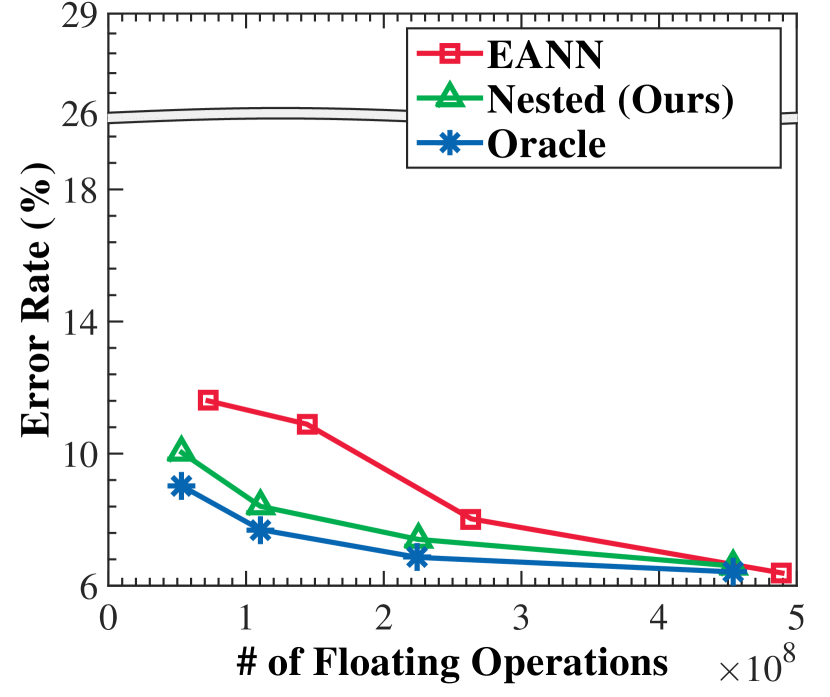
(a) Depth-nested;
Sparse ResNet-98

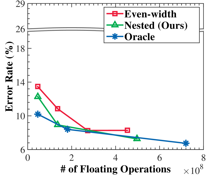
(b) Width-nested;
ResNet-42

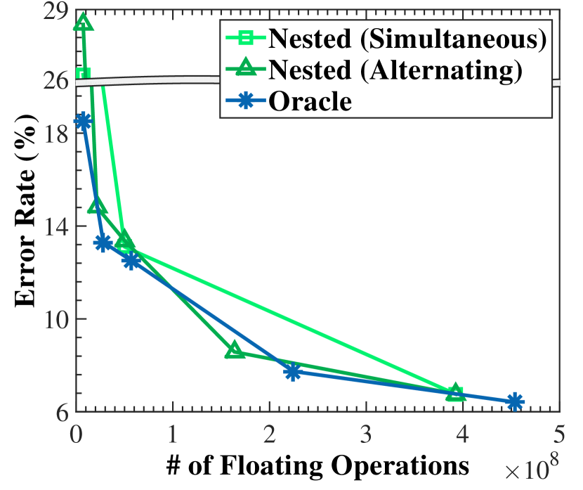
(c) Width-depth;
Sparse ResNet-98

Figure 9: Accuracy-FLOP trade-offs (lower is better). Our nested architectures offer trade-offs close to the infeasible Oracle.

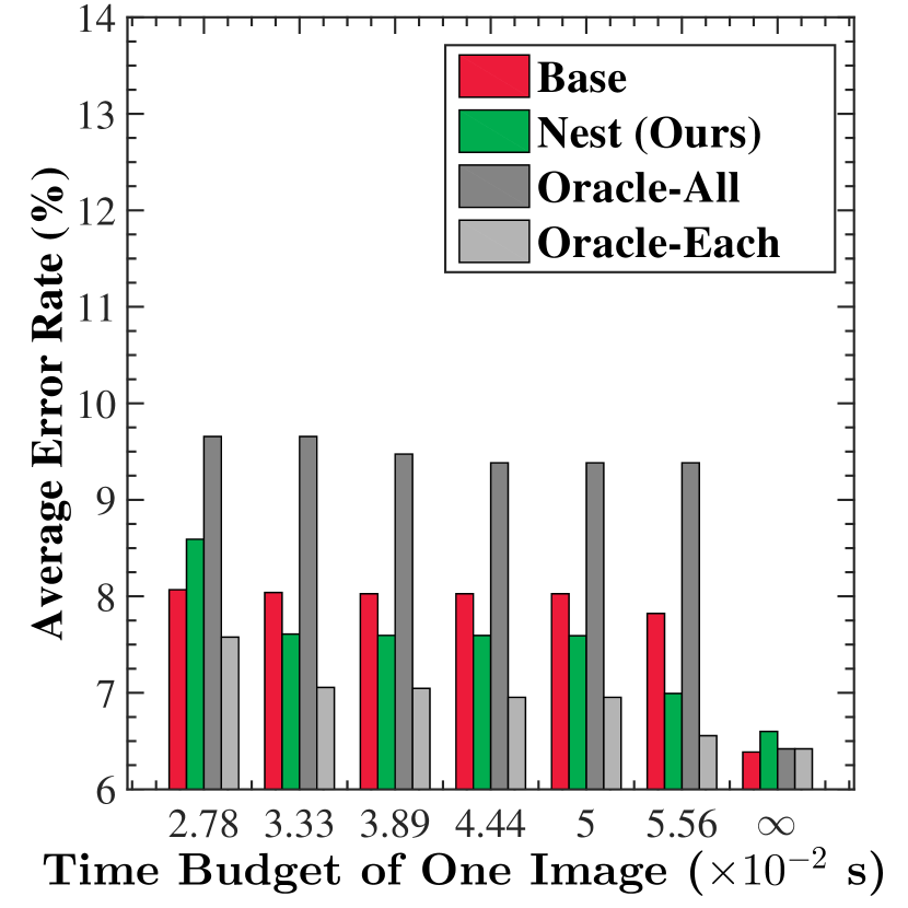
(a) Depth-nested;
Sparse ResNet-98

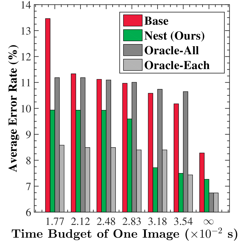
(b) Width-nested;
ResNet-42

(c) Width-depth;
Sparse ResNet-98

Figure 10: Error rates at different deadlines (lower is better). Our nested designs perform better than baselines and the static Oracle.

We compare our nested architectures to an infeasible Oracle—a collection of independently-trained single-task networks with sizes matching our subnetwork stages. Perfectly deploying this collection of independent networks as an anytime system would require oracle knowledge of impending deadlines to select which network to run. The Oracle thus represents an impossible scenario in which anytime prediction capability is granted for free. Figure 10 shows the accuracy-FLOPs trade-off curves achieved by our nested network designs (green), the Oracle (blue), and the EANN and Even-width baselines (red). Here, each network is trained using the strategy that offers the most accurate results (i.e., OSGD for all anytime networks and SGD for all independent networks except for the largest setting of SparseResNet-98, which uses NormSGD).

From Figure 10a and 10b, our depth and width nesting anytime networks both offer much better accuracy-FLOPs trade-offs than previous work, and come close to the infeasible Oracle. Figure 10c shows our width-depth nested Sparse ResNet-98 offers almost as good a trade-off as the Oracle, and covers a much wider trade-off spectrum than depth-only or width-only nesting.

5.4 Run-time Simulation

We further compare four schemes for maximizing inference accuracy under various inference deadlines: (1) Baseline anytime schemes (Even-width and EANN); (2) Our Nested anytime schemes (width, depth, and width-depth nesting). (3) Oracle${}_{\text{All}}$, which picks the most accurate independent network that finishes before the deadline for all inputs; (4) Oracle${}_{\text{Each}}$, which picks the most accurate independent network for each input that finishes before the deadline (i.e., the network may vary across inputs). When no inference result is generated by the deadline, a random guess is output. We report the average error rates across all inputs in Figure 10 (vertical axis, lower is better) under 7 deadlines and then no deadline (horizontal axis); the 7 deadlines are set to be 0.5x-1x of the average latency under the biggest ResNet-42 or Sparse ResNet across all inputs.

The accuracy advantage of Nest (the second bar in each group) over Base (the first bar), and Oracle${}_{\text{All}}$ (the third bar) is apparent in Figure 10. For example, for ResNet-42, Nest has 7%-24% lower error rate than Base for all deadlines. Nest has lower accuracy than Oracle${}_{\text{Each}}$ in most cases, because the anytime network usually has slightly lower accuracy than an independent network with same size. Note that Oracle${}_{\text{Each}}$ is impractical, as it assumes impossible latency prediction and no-overhead in swapping networks across inputs. These accuracy-under-deadline results are consistent with the accuracy-latency curves in Figure 10.

5.5 Evaluation on ImageNet

Finally, we train a width-nested ResNet-50 and depth-nested Sparse ResNet-66 on the large-scale ImageNet (ILSVRC 2012) dataset (Deng et al., 2009), using both SGD and OSGD. All networks are trained for 90 epochs, with learning rate decreasing from 0.1 to 0.0001. Table 3 reports top-1 and top-5 validation error rates. These results are consistent with our previous findings on CIFAR. On ImageNet, OSGD significantly improves the accuracy of later stages (larger subnetworks) compared to standard SGD.

	SGD		OSGD
	Top-1 Error	Top-5 Error	Top-1 Error	Top-5 Error
Our Width Nested ResNet-50
1w1	36.7	14.7	36.7	14.8
2w2	31.5	11.7	31.7	11.7
3w4	29.2	10.2	28.3	9.4
Our Depth Nested Sparse ResNet-66
1d1	31.3	11.3	32.9	12.4
2d2	28.4	9.7	29.2	10.1
3d4	28.0	9.3	27.1	8.9

Table 3: Validation error of anytime networks trained with SGD and OSGD on the ImageNet dataset. As was the case for CIFAR-10 (Table 1), OSGD improves the accuracy of later output stages.

6 Conclusion

We propose a new class of neural network architectures, which recursively nest subnetworks in both width and depth. We also propose Orthogonalized SGD, a novel variant of SGD customized for training such architectures with re-balanced task-specific gradients. We evaluate them with a variety of network designs and achieve high accuracy and run-time flexibility. Our experiments demonstrate synergy between our architecture and optimizer: our anytime networks perform almost as well as independent non-anytime networks of the same size.

Acknowledgments. This work is supported by NSF (grants CNS-1764039, CNS-1764039, CNS-1514256, CNS-1823032), ARO (grant W911NF1920321), DOE (grant DESC0014195 0003), and the CERES Center for Unstoppable Computing. Continuing support for this line of research is provided in part by NSF grant CNS-1956180.

References

- Bilen & Vedaldi (2017) Bilen, H. and Vedaldi, A. Universal representations: The missing link between faces, text, planktons, and cat breeds. arXiv:1701.07275, 2017.
- Bucilua et al. (2006) Bucilua, C., Caruana, R., and Niculescu-Mizil, A. Model compression. In SIGKDD, 2006.
- Caruana (1997) Caruana, R. Multitask learning. Machine learning, 1997.
- Chen et al. (2015) Chen, C., Seff, A., Kornhauser, A., and Xiao, J. DeepDriving: Learning affordance for direct perception in autonomous driving. In ICCV, 2015.
- Chen et al. (2017) Chen, Z., Badrinarayanan, V., Lee, C.-Y., and Rabinovich, A. Gradnorm: Gradient normalization for adaptive loss balancing in deep multitask networks. arXiv:1711.02257, 2017.
- Collobert & Weston (2008) Collobert, R. and Weston, J. A unified architecture for natural language processing: Deep neural networks with multitask learning. In ICML, 2008.
- Deng et al. (2009) Deng, J., Dong, W., Socher, R., Li, L., Li, K., and Fei-Fei, L. ImageNet: A large-scale hierarchical image database. In CVPR, 2009.
- Devlin et al. (2018) Devlin, J., Chang, M.-W., Lee, K., and Toutanova, K. BERT: Pre-training of deep bidirectional transformers for language understanding. arXiv:1810.04805, 2018.
- Dietterich (2000) Dietterich, T. G. Ensemble methods in machine learning. In MCS, 2000.
- Dollar et al. (2011) Dollar, P., Wojek, C., Schiele, B., and Perona, P. Pedestrian detection: An evaluation of the state of the art. TPAMI, 2011.
- Donahue et al. (2014) Donahue, J., Jia, Y., Vinyals, O., Hoffman, J., Zhang, N., Tzeng, E., and Darrell, T. Decaf: A deep convolutional activation feature for generic visual recognition. In ICML, 2014.
- Dosovitskiy et al. (2017) Dosovitskiy, A., Ros, G., Codevilla, F., Lopez, A., and Koltun, V. CARLA: An open urban driving simulator. In CoRL, 2017.
- Eigen & Fergus (2015) Eigen, D. and Fergus, R. Predicting depth, surface normals and semantic labels with a common multi-scale convolutional architecture. In CVPR, 2015.
- Farajtabar et al. (2020) Farajtabar, M., Azizan, N., Mott, A., and Li, A. Orthogonal gradient descent for continual learning. In International Conference on Artificial Intelligence and Statistics, 2020.
- Figurnov et al. (2017) Figurnov, M., Collins, M. D., Zhu, Y., Zhang, L., Huang, J., Vetrov, D. P., and Salakhutdinov, R. Spatially adaptive computation time for residual networks. In CVPR, 2017.
- Fowers et al. (2018) Fowers, J., Ovtcharov, K., Papamichael, M., Massengill, T., Liu, M., Lo, D., Alkalay, S., Haselman, M., Adams, L., Ghandi, M., et al. A configurable cloud-scale DNN processor for real-time AI. In ISCA. IEEE Press, 2018.
- Greff et al. (2017) Greff, K., Srivastava, R. K., and Schmidhuber, J. Highway and residual networks learn unrolled iterative estimation. In ICLR, 2017.
- Grubb & Bagnell (2012) Grubb, A. and Bagnell, D. SpeedBoost: Anytime prediction with uniform near-optimality. In AISTATS, 2012.
- Han et al. (2016) Han, S., Mao, H., and Dally, W. J. Deep compression: Compressing deep neural networks with pruning, trained quantization and huffman coding. In ICLR, 2016.
- Hashimoto et al. (2016) Hashimoto, K., Xiong, C., Tsuruoka, Y., and Socher, R. A joint many-task model: Growing a neural network for multiple NLP tasks. arXiv:1611.01587, 2016.
- He et al. (2016) He, K., Zhang, X., Ren, S., and Sun, J. Deep residual learning for image recognition. In CVPR, 2016.
- Hinton et al. (2015) Hinton, G., Vinyals, O., and Dean, J. Distilling the knowledge in a neural network. arXiv:1503.02531, 2015.
- Hoffmann & Maggio (2014) Hoffmann, H. and Maggio, M. PCP: A generalized approach to optimizing performance under power constraints through resource management. In ICAC, 2014.
- Howard et al. (2017) Howard, A. G., Zhu, M., Chen, B., Kalenichenko, D., Wang, W., Weyand, T., Andreetto, M., and Adam, H. MobileNets: Efficient convolutional neural networks for mobile vision applications. arXiv:1704.04861, 2017.
- Hu et al. (2019) Hu, H., Dey, D., Hebert, M., and Bagnell, J. A. Learning anytime predictions in neural networks via adaptive loss balancing. In AAAI, 2019.
- Huang et al. (2017a) Huang, G., Chen, D., Li, T., Wu, F., van der Maaten, L., and Weinberger, K. Q. Multi-scale dense convolutional networks for efficient prediction. In CoRR, 2017a.
- Huang et al. (2017b) Huang, G., Liu, Z., Van Der Maaten, L., and Weinberger, K. Q. Densely connected convolutional networks. In CVPR, 2017b.
- Huval et al. (2015) Huval, B., Wang, T., Tandon, S., Kiske, J., Song, W., Pazhayampallil, J., Andriluka, M., Rajpurkar, P., Migimatsu, T., Cheng-Yue, R., et al. An empirical evaluation of deep learning on highway driving. arXiv:1504.01716, 2015.
- Iandola et al. (2016) Iandola, F. N., Han, S., Moskewicz, M. W., Ashraf, K., Dally, W. J., and Keutzer, K. SqueezeNet: AlexNet-level accuracy with 50x fewer parameters and 0.5MB model size. arXiv:1602.07360, 2016.
- Jastrzebski et al. (2018) Jastrzebski, S., Arpit, D., Ballas, N., Verma, V., Che, T., and Bengio, Y. Residual connections encourage iterative inference. In ICLR, 2018.
- Kendall et al. (2018) Kendall, A., Gal, Y., and Cipolla, R. Multi-task learning using uncertainty to weigh losses for scene geometry and semantics. In CVPR, 2018.
- Kokkinos (2017) Kokkinos, I. UberNet: Training a universal convolutional neural network for low-, mid-, and high-level vision using diverse datasets and limited memory. In CVPR, 2017.
- Krizhevsky & Hinton (2012) Krizhevsky, A. and Hinton, G. Learning multiple layers of features from tiny images. Technical report, University of Toronto, 2012.
- Larsson (2017) Larsson, G. Discovery of visual semantics by unsupervised and self-supervised representation learning. arXiv:1708.05812, 2017.
- Larsson et al. (2017) Larsson, G., Maire, M., and Shakhnarovich, G. FractalNet: Ultra-deep neural networks without residuals. In ICLR, 2017.
- Lee & Shin (2018) Lee, H. and Shin, J. Anytime neural prediction via slicing networks vertically. arXiv:1807.02609, 2018.
- Lin et al. (2018) Lin, S.-C., Zhang, Y., Hsu, C.-H., Skach, M., Haque, M. E., Tang, L., and Mars, J. The architectural implications of autonomous driving: Constraints and acceleration. In ASPLOS, 2018.
- Long & Wang (2015) Long, M. and Wang, J. Learning multiple tasks with deep relationship networks. arXiv:1506.02117, 2, 2015.
- McGill & Perona (2017) McGill, M. and Perona, P. Deciding how to decide: Dynamic routing in artificial neural networks. In ICML, 2017.
- Misra et al. (2016) Misra, I., Shrivastava, A., Gupta, A., and Hebert, M. Cross-stitch networks for multi-task learning. In CVPR, 2016.
- Pham et al. (2018) Pham, H., Guan, M., Zoph, B., Le, Q., and Dean, J. Efficient neural architecture search via parameters sharing. In ICML, 2018.
- Rastegari et al. (2016) Rastegari, M., Ordonez, V., Redmon, J., and Farhadi, A. XNOR-Net: ImageNet classification using binary convolutional neural networks. In ECCV, 2016.
- Ren et al. (2018) Ren, M., Pokrovsky, A., Yang, B., and Urtasun, R. SBNet: Sparse blocks network for fast inference. In CVPR, 2018.
- Seltzer & Droppo (2013) Seltzer, M. L. and Droppo, J. Multi-task learning in deep neural networks for improved phoneme recognition. In ICASSP, 2013.
- Simonyan & Zisserman (2015) Simonyan, K. and Zisserman, A. Very deep convolutional networks for large-scale image recognition. In ICLR, 2015.
- Søgaard & Goldberg (2016) Søgaard, A. and Goldberg, Y. Deep multi-task learning with low level tasks supervised at lower layers. In ACL, 2016.
- Szegedy et al. (2015) Szegedy, C., Liu, W., Jia, Y., Sermanet, P., Reed, S., Anguelov, D., Erhan, D., Vanhoucke, V., and Rabinovich, A. Going deeper with convolutions. In CVPR, 2015.
- Teerapittayanon et al. (2016) Teerapittayanon, S., McDanel, B., and Kung, H. BranchyNet: Fast inference via early exiting from deep neural networks. In ICPR, 2016.
- Teichmann et al. (2018) Teichmann, M., Weber, M., Zoellner, M., Cipolla, R., and Urtasun, R. MultiNet: Real-time joint semantic reasoning for autonomous driving. In IV, 2018.
- Veit & Belongie (2018) Veit, A. and Belongie, S. Convolutional networks with adaptive inference graphs. In ECCV, 2018.
- Viola & Jones (2004) Viola, P. and Jones, M. J. Robust real-time face detection. IJCV, 2004.
- Wang et al. (2019) Wang, Y., Lai, Z., Huang, G., Wang, B. H., van der Maaten, L., Campbell, M., and Weinberger, K. Q. Anytime stereo image depth estimation on mobile devices. In ICRA, 2019.
- Wu et al. (2015) Wu, Z., Valentini-Botinhao, C., Watts, O., and King, S. Deep neural networks employing multi-task learning and stacked bottleneck features for speech synthesis. In ICASSP, 2015.
- Wu et al. (2018) Wu, Z., Nagarajan, T., Kumar, A., Rennie, S., Davis, L. S., Grauman, K., and Feris, R. BlockDrop: Dynamic inference paths in residual networks. In CVPR, 2018.
- Xie et al. (2019) Xie, S., Zheng, H., Liu, C., and Lin, L. SNAS: Stochastic neural architecture search. In ICLR, 2019.
- Xu et al. (2012) Xu, Z., Weinberger, K., and Chapelle, O. The greedy miser: Learning under test-time budgets. In ICML, 2012.
- Xu et al. (2013) Xu, Z., Kusner, M., Weinberger, K., and Chen, M. Cost-sensitive tree of classifiers. In ICML, 2013.
- Yang & Hospedales (2017) Yang, Y. and Hospedales, T. Deep multi-task representation learning: A tensor factorisation approach. In ICLR, 2017.
- Zagoruyko & Komodakis (2016) Zagoruyko, S. and Komodakis, N. Wide residual networks. In BMVC, 2016.
- Zamir et al. (2018) Zamir, A. R., Sax, A., Shen, W., Guibas, L. J., Malik, J., and Savarese, S. Taskonomy: Disentangling task transfer learning. In CVPR, 2018.
- Zhu et al. (2018) Zhu, L., Deng, R., Maire, M., Deng, Z., Mori, G., and Tan, P. Sparsely aggregated convolutional networks. In ECCV, 2018.
- Zhuravlev et al. (2010) Zhuravlev, S., Blagodurov, S., and Fedorova, A. Addressing shared resource contention in multicore processors via scheduling. In ASPLOS, 2010.
- Zilberstein (1996) Zilberstein, S. Using anytime algorithms in intelligent systems. AI magazine, 1996.
- Zoph & Le (2017) Zoph, B. and Le, Q. V. Neural architecture search with reinforcement learning. In ICLR, 2017.