A Scalable, Adaptive and Sound Nonconvex Regularizer for Low-rank Matrix Learning

Abstract.

Matrix learning is at the core of many machine learning problems. A number of real-world applications such as collaborative filtering and text mining can be formulated as a low-rank matrix completion problems, which recovers incomplete matrix using low-rank assumptions. To ensure that the matrix solution has a low rank, a recent trend is to use nonconvex regularizers that adaptively penalize singular values. They offer good recovery performance and have nice theoretical properties, but are computationally expensive due to repeated access to individual singular values. In this paper, based on the key insight that adaptive shrinkage on singular values improve empirical performance, we propose a new nonconvex low-rank regularizer called ”nuclear norm minus Frobenius norm” regularizer, which is scalable, adaptive and sound. We first show it provably holds the adaptive shrinkage property. Further, we discover its factored form which bypasses the computation of singular values and allows fast optimization by general optimization algorithms. Stable recovery and convergence are guaranteed. Extensive low-rank matrix completion experiments on a number of synthetic and real-world data sets show that the proposed method obtains state-of-the-art recovery performance while being the fastest in comparison to existing low-rank matrix learning methods.

1. Introduction

In many real-world scenarios, the data can be naturally represented as matrices. Examples include the rating matrices in recommender systems (Srebro et al., 2005; Koren et al., 2009; Candès and Recht, 2009; Li et al., 2018; Sharma and Karypis, 2019), the term-document matrices of texts in natural language processing (Pennington et al., 2014; Shi et al., 2018), images in computer vision (Hu et al., 2012; Gu et al., 2014), and climate observations in spatial-temporal analysis (Bahadori et al., 2014). Thus, matrix learning is an important and fundamental tool in machine learning (Srebro et al., 2005; Candes et al., 2008; Chen et al., 2011), data mining (Koren et al., 2009; Bahadori et al., 2014), and computer vision (Gu et al., 2014; Yao et al., 2019).

In this paper, we focus on an important class of matrix learning problems, namely matrix completion, which tries to predict the missing entries of a partially observed matrix (Candes et al., 2008). For example, in collaborative filtering (Koren et al., 2009), the rating matrix is often incomplete and one wants to predict the missing user ratings for all items. In climate analysis (Bahadori et al., 2014), observation records from only a few meteorological stations are available, and one wants to predict climate information for the other locations. In image inpainting (Hu et al., 2012; Gu et al., 2014), the image has pixels missing and one wants to fill in these missing values. To avoid the problem to be ill-posed, the target matrix is often assumed to have a low rank (Candès and Recht, 2009). To obtain such a solution, a direct approach is to add a rank-minimizing term to the optimization objective. However, rank minimization is NP-hard (Candès and Recht, 2009). Thus, computationally, a more feasible approach is to use a regularizer that encourages the target matrix to have a small rank.

There exist various low-rank regularizers. Nuclear norm regularizer is the tightest convex surrogate for matrix rank (Candès and Recht, 2009), which has good recovery and convergence guarantees. Defined as the sum of singular values, nuclear norm requires repeatedly computing the singular value decomposition (SVD), which is expensive. To be more efficient, a series of works instead turn to matrix factorization which factorizes the recovered matrix into factor matrices. Some of them work towards theoretical justification (Tu et al., 2016; Wang et al., 2017), while the other targets at designing better algorithms (Vandereycken, 2013; Boumal and Absil, 2015; Gunasekar et al., 2017). However, the performance of matrix factorization is not satisfactory (Fan et al., 2019; Yao et al., 2019). To this end, factored low-rank regularizers are invented to balance efficiency and effectiveness, such as factored nuclear norm (Srebro et al., 2005) and factored group-sparse regularizer (GSR) (Fan et al., 2019). It is proved that factored nuclear norm can obtain comparable result as nuclear norm under mild condition (Srebro et al., 2005).

Recently, nonconvex low-rank regularizers (Table 1) which penalize less on the more informative large singular values are proposed, such as Schatten-p norm (Nie et al., 2012), truncated $\ell_{1\text{-}2}$ norm (Ma et al., 2017), capped-$\ell_{1}$ penalty (Zhang, 2010b), log-sum penalty (LSP) (Candes et al., 2008), and minimax concave penalty (MCP) (Zhang, 2010a). These nonconvex regularizers can outperform nuclear norm both theoretically (Gui et al., 2016; Mazumder et al., 2020) and empirically (Lu et al., 2015a, b; Yao et al., 2019). However, as shown in Table 1, none of the above-mentioned regularizers obtain (A) scalability, (B) good performance and (C-D) sound theoretical guarantee simultaneously.

Table 1. Comparisons among nonconvex low-rank regularizers on (A): Scalability (can be optimized in factored form); (B): Performance (can adaptively penalize singular values); (C): Statistical guarantee; (D): Convergence guarantee.

nonconvex low-rank regularizer	expression	(A)	(B)	(C)	(D)
factored nuclear norm (Srebro et al., 2005)	$\min_{\mathbf{X}=\mathbf{W}\mathbf{H}^{\top}}\frac{\lambda}{2}(\|\mathbf{W}\|_{F}^{2}+\|\mathbf{H}\|_{F}^{2})$	✓	✗	✓	✓
Schatten-p (Nie et al., 2012)	$\lambda(\sum_{i=1}^{m}\sigma^{p}_{i}(\mathbf{X}))^{1/p}$	✗	✗	✓	✓
factored GSR (Fan et al., 2019)	$\min_{\mathbf{X}=\mathbf{W}\mathbf{H}^{\top}}\frac{\lambda}{2}(\|\mathbf{W}\|_{2,1}+\|\mathbf{H}^{\top}\|_{2,1})$	✓	✗	✓	✓
capped-$\ell_{1}$, LSP, and MCP (Lu et al., 2015b; Yao et al., 2019)	$\lambda\sum_{i=1}^{m}\hat{r}(\sigma_{i}(\mathbf{X}))$ (see $\hat{r}$ in Table 2)	✗	✓	✓	✓
truncated $\ell_{1\text{-}2}$ (Ma et al., 2017)	$\sum\nolimits_{i=t+1}^{n}\sigma_{i}(\mathbf{X})-(\sum\nolimits_{i=t+1}^{n}\sigma^{2}_{i}(\mathbf{X}))^{\nicefrac{{1}}{{2}}}$	✗	✓	✓	✓
NNFN	$\|\mathbf{X}\|_{*}-\|\mathbf{X}\|_{F}$	✗	✓	✓	✓
factored NNFN	$\min_{\mathbf{X}=\mathbf{W}\mathbf{H}^{\top}}\frac{\lambda}{2}(\|\mathbf{W}\|_{F}^{2}\!+\!\|\mathbf{H}\|_{F}^{2})\!-\!\lambda\|\mathbf{W}\mathbf{H}^{\top}\|_{F}$	✓	✓	✓	✓

To fill in this blank, we propose a scalable, adaptive and sound nonconvex regularizer based on the key insight that adaptive shrinkage property of common nonconvex regularizers can improve empirical performance. Specifically, Our contribution can be summarized as follows:

• We propose a new nonconvex regularizer called ”nuclear norm minus Frobenius norm” (NNFN) regularizer for low-rank matrix learning, which is scalable, adaptive and theoretically guaranteed.

• We show that NNFN regularizer can be factorized to sidestep the expensive SVD. This problem can be optimized by general algorithms such as gradient descent.

• We provide sound theoretical analysis on statistical and convergence properties of both NNFN and factored NNFN regularizers.

• We conduct extensive experiments on both synthetic and a number of real-world data sets including recommendation data and climate record data. In comparison to existing methods, results consistently show that the proposed algorithm obtains state-of-the-art recovery performance while being the fastest.

Notations: Vectors are denoted by lowercase boldface, matrices by uppercase boldface. $(\cdot)^{\top}$ denotes transpose operation and $\mathbf{A}_{+}\!=\![\max(A_{ij},0)]$. For a vector $\mathbf{x}=[x_{i}]\in\mathbb{R}^{m}$, $\text{Diag}(\mathbf{x})$ constructs a $m\times m$ diagonal matrix with the $i$th diagonal element being $x_{i}$. $\mathbf{I}$ denotes the identity matrix. For a square matrix $\mathbf{X}$, $\text{tr}(\mathbf{X})$ is its trace. For matrix $\mathbf{X}\in\mathbb{R}^{m\times n}$ (without loss of generality, we assume that $m\geq n$), $\|\mathbf{X}\|_{F}=\sqrt{\text{tr}(\mathbf{X}^{\top}\mathbf{X})}$ is its Frobenius norm. Let the singular value decomposition (SVD) of a rank-$k^{*}$ $\mathbf{X}$ be $\mathbf{U}\text{Diag}(\bm{\sigma}(\mathbf{X}))\mathbf{V}^{\top}$, where $\mathbf{U}\in\mathbb{R}^{m\times k^{*}}$, $\mathbf{V}\in\mathbb{R}^{n\times k^{*}}$, $\bm{\sigma}(\mathbf{X})=[\sigma_{i}(\mathbf{X})]\in\mathbb{R}^{k^{*}}$ with $\sigma_{i}(\mathbf{X})$ being the $i$th singular value of $\mathbf{X}$ and $\sigma_{1}(\mathbf{X})\geq\sigma_{2}(\mathbf{X})\geq\dots\geq\sigma_{k}(\mathbf{X})\geq 0$.

2. Background: Low-Rank Matrix Learning

As minimizing the rank is NP-hard (Candès and Recht, 2009), low-rank matrix learning is often formulated as the following optimization problem:

(1) $$\min\nolimits_{\mathbf{X}}f(\mathbf{X})+\lambda r(\mathbf{X}),$$

where $f$ is a smooth function (usually the loss), $r(\mathbf{X})$ is a regularizer that encourages $\mathbf{X}$ to be low-rank, and $\lambda\geq 0$ is a tradeoff hyperparameter. Let $\mathbf{\Omega}\in\{0,1\}^{m\times n}$ record positions of the observed entries (with $\Omega_{ij}=1$ if $O_{ij}$ is observed, and $0$ otherwise), and $\mathcal{P}_{\mathbf{\Omega}}(\cdot)$ is a projection operator such that $[\mathcal{P}_{\mathbf{\Omega}}(\mathbf{A})]_{ij}=A_{ij}$ if $\Omega_{ij}=1$ and $0$ otherwise. Low-rank matrix completion (Candès and Recht, 2009) tries to recover the underlying low-rank matrix $\mathbf{X}\in\mathbb{R}^{m\times n}$ from an incomplete matrix $\mathbf{O}\in\mathbb{R}^{m\times n}$ with only a few observed entries. It usually sets $f(\mathbf{X})$ as

(2) $$f(\mathbf{X})\equiv\frac{1}{2}\|\mathcal{P}_{\mathbf{\Omega}}(\mathbf{X}-\mathbf{O})\|_{F}^{2},$$

which measures the recovery error.

2.1. Convex Nuclear Norm Regularizer

The convex nuclear norm $\|\mathbf{X}\|_{*}=\|\bm{\sigma}(\mathbf{X})\|_{1}$ (Candès and Recht, 2009), is the tightest convex surrogate of the matrix rank (Fazel, 2002). Problem (1) is usually solved by the proximal algorithm (Parikh and Boyd, 2014). At the $t$th iteration, it generates the next iterate by computing the proximal step $\mathbf{X}_{t+1}=\text{prox}_{\eta\lambda r}(\mathbf{X}_{t}-\eta\lambda\nabla(\mathbf{X}_{t}))$, where $\eta>0$ is the stepsize, and $\text{prox}_{\lambda r}(\mathbf{Z})=\arg\min_{\mathbf{X}}\frac{1}{2}\|\mathbf{X}-\mathbf{Z}\|_{2}^{2}+\lambda r(\mathbf{X})$ is the proximal operator. In general, the proximal operator should be easily computed. For the nuclear norm, its proximal operator is computed as (Cai et al., 2010):

(3) $$\text{prox}_{\lambda\|\cdot\|_{*}}(\mathbf{Z})=\mathbf{U}\left(\text{Diag}(\bm{\sigma}(\mathbf{Z}))-\lambda\mathbf{I}\right)_{+}\mathbf{V}^{\top},$$

where $\mathbf{U}\text{Diag}(\bm{\sigma}(\mathbf{Z}))\mathbf{V}^{\top}$ is the SVD of $\mathbf{Z}$.

2.2. Nonconvex Regularizers

Recently, various nonconvex regularizers appear (Table 1). Common examples include the capped-$\ell_{1}$ penalty (Zhang, 2010b), log-sum penalty (LSP) (Candes et al., 2008), and minimax concave penalty (MCP) (Zhang, 2010a).

Table 2. Nonconvex low-rank regularizers in the form of (4).

	$\hat{r}(\sigma_{i}(\mathbf{X}))$
capped-$\ell_{1}$	$\min(\sigma_{i}(\mathbf{X}),\theta)$
LSP	$\log\left(\frac{1}{\theta}\sigma_{i}(\mathbf{X})+1\right)$
MCP	$\begin{cases}\sigma_{i}(\mathbf{X})-\frac{\sigma_{i}^{2}(\mathbf{X})}{2\theta\lambda}&\text{if}\;\sigma_{i}(\mathbf{X})\leq\theta\lambda\\ \frac{\theta\lambda}{2}&\text{otherwise}\end{cases}$

As shown in Table 2, they can be written in the general form of

(4) $$r(\mathbf{X})=\sum\nolimits_{i=1}^{n}\hat{r}(\sigma_{i}(\mathbf{X})),$$

where $\hat{r}(\alpha)$ is nonlinear, concave and non-decreasing for $\alpha\geq 0$ with $\hat{r}(0)=0$. In contrast to the proximal operator in (3) which penalizes all singular values of $\mathbf{Z}$ by the same amount $\lambda$, these nonconvex regularizers penalize less on the larger singular values which are more informative. Additionally, the nonconvex Schatten-p norm (Nie et al., 2012) can better approximate rank than nuclear norm. Truncated $\ell_{1\text{-}2}$ regularizer (Ma et al., 2017) can obtain unbiased approximation for rank (Ma et al., 2017). These nonconvex regularizers outperform nuclear norm on many applications empirically (Gu et al., 2014; Lu et al., 2015b; Yao et al., 2019), and can obtain lower recovery errors (Gui et al., 2016). However, learning with nonconvex regularizers is very difficult. It usually requires dedicated solvers to leverage special structures (such as the low-rank-plus-sparse structure in (Hastie et al., 2015; Yao et al., 2019)) or involves several iterative algorithms (such as the difference of convex functions algorithm (DCA) (Hiriart-Urruty, 1985) with subproblems solved by the alternating direction method of multipliers (ADMM) (Boyd et al., 2011) for truncated $\ell_{1\text{-}2}$ regularized problem). This computation bottleneck limits their applications in practice.

2.3. Factored Regularizers

Note that aforementioned regularizers require access to individual singular values. As computing the singular values of a $m\times n$ matrix (with $m\geq n$) via SVD takes $O(mn^{2})$ time, this can be costly for a large matrix. Even when rank-$k$ truncated SVD is used, the computation cost is still $O(mnk)$. To relieve the computational burden, factored low-rank regualrizers are invented. (1) can then be rewritten into a factored form as

(5) $$\min\nolimits_{\mathbf{W},\mathbf{H}}f(\mathbf{W}\mathbf{H}^{\top})+\mu g(\mathbf{W},\mathbf{H}),$$

where $\mathbf{X}$ is factorized into $\mathbf{W}\in\mathbb{R}^{m\times k}$ and $\mathbf{H}\in\mathbb{R}^{n\times k}$, and $\mu\geq 0$ is a hyperparameter. When $\mu=0$, this reduces to matrix factorization (Vandereycken, 2013; Boumal and Absil, 2015; Tu et al., 2016; Wang et al., 2017; Gunasekar et al., 2017). Not all regularizers $r(\mathbf{X})$ have equivalent factored form $g(\mathbf{W},\mathbf{H})$. For a matrix $\mathbf{X}$ with rank $k^{*}\leq k$, it is already discovered that nuclear norm can be rewritten in a factored form (Srebro et al., 2005) as $\|\mathbf{X}\|_{*}=\min_{\mathbf{X}=\mathbf{W}\mathbf{H}^{\top}}\nicefrac{{1}}{{2}}(\|\mathbf{W}\|_{F}^{2}+\|\mathbf{H}\|_{F}^{2})$. As for nonconvex low-rank regularizers, only Schatten-p norm can be approximated by factored forms (Shang et al., 2016; Fan et al., 2019). Other nonconvex regularizers, which need to penalize individual singular values, cannot be written in factored form.

3. Nuclear Norm Minus Frobenius Norm (NNFN) Regularizer

Based on the insight that adaptive shrinkage on singular values can improve empirical performance, we present a new nonconvex regularizer

(6) $$r_{\text{NNFN}}(\mathbf{X})=\|\mathbf{X}\|_{*}-\|\mathbf{X}\|_{F},$$

which will be called the “nuclear norm minus Frobenius norm” (NNFN) regularizer. Next, we will show that NNFN regularizer applies adaptive shrinkage for singular values provably, has factored form which allows fast optimization by general algorithms, and has sound theoretically guarantee.

3.1. Adaptive Shrinkage Property

Recall from (3) that the proximal operator of the nuclear norm equally penalizes each singular value by $\lambda$ until it reaches zero. In contrast, we find that common noncovex regularizers $r(\mathbf{X})$ of the general form (4) all hold the adaptive shrinkage property in Proposition 1.

Proposition 1 (Adaptive Shrinkage Property).

Let $r(\mathbf{X})$ be a nonconvex low-rank regularizer of the form (4), and $\tilde{\bm{\sigma}}=[\tilde{\sigma}_{i}]=\text{prox}_{\lambda r(\cdot)}(\bm{\sigma}(\mathbf{Z}))$ in (7). Then, (i) ${\sigma}_{i}(\mathbf{Z})\!\geq\!\tilde{\sigma}_{i}$ (shrinkage); and (ii) $\sigma_{i}(\mathbf{Z})\!-\!\tilde{\sigma}_{i}\!\leq\!\sigma_{i+1}(\mathbf{Z})\!-\!\tilde{\sigma}_{i+1}$ (adaptivity), where strict inequality holds at least for one $i$.

It shows that $\text{prox}_{\lambda r}(\cdot)$ adaptively shrinks the singular values of its matrix argument, in that larger singular values are penalized less. This property is important for obtaining good empirical performance (Gu et al., 2014; Hu et al., 2012; Lu et al., 2015b, a; Yao et al., 2019). Other nonconvex regularizers such as truncated $\ell_{1\text{-}2}$ and Schatten-p norm, do not have this property due to the lack of analytic proximal operators. Figure 1 shows the shrinkage performed by adaptive nonconvex regularizers versus the convex nuclear norm regularizer. As can be seen, the convex nuclear norm regularizer shrinks all singular values by the same amount; whereas the adaptive nonconvex regularizers enforce different amounts of shrinkage depending on the magnitude of $\sigma_{i}(\mathbf{Z})$.

Figure 1. Shrinkage performed by different regularizers. The hyperparameters are tuned such that $\tilde{\sigma}_{i}$ is zero for $\sigma_{i}(\mathbf{Z})\leq 5$.

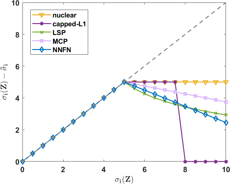
Here, we show the proposed NNFN regularizer in (6) also provably satisfies adaptive shrinkage of the singular values when used with a proximal algorithm. We first present the proximal operator of $r_{\text{NNFN}}(\cdot)$ in Proposition 2. As $\text{prox}_{\lambda\|\cdot\|_{1\text{-}2}}(\bm{\sigma}(\mathbf{Z}))$ returns a sparse vector (Lou and Yan, 2018), the resultant $\text{prox}_{\lambda r_{\text{NNFN}}}(\mathbf{Z})$ is low-rank.

Proposition 2.

Given a matrix $\mathbf{Z}$, let its SVD be $\bar{\mathbf{U}}\text{Diag}({\bm{\sigma}}(\mathbf{Z}))\bar{\mathbf{V}}^{\top}$, and $\lambda\leq\|\bm{\sigma}(\mathbf{Z})\|_{\infty}$.

(7) $$\text{prox}_{\lambda r_{\text{NNFN}}}(\mathbf{Z})=\bar{\mathbf{U}}\text{Diag}(\text{prox}_{\lambda\|\cdot\|_{1\text{-}2}}(\bm{\sigma}(\mathbf{Z})))\bar{\mathbf{V}}^{\top},$$

where $\text{prox}_{\lambda\|\cdot\|_{1\text{-}2}}(\mathbf{z})$ has closed-form solution (Lou and Yan, 2018).

Now, we are ready to prove in the following Corollary that NNFN regularizer also shares the adaptive shrinkage property. This can lead to better empirical performance as discussed earlier.

Corollary 3.

The two properties in Proposition 1 also hold for the proximal operators of the NNFN regularizer.

4. Algorithms for (1) with NNFN Regularizer

With the proximal operator obtained in Proposition 2, learning with the NNFN regularizer can be readily solved with the proximal algorithm. However, it still relies on computing the SVD in each iteration. To tackle this problem, we then present a simple and scalable algorithm that avoids SVD computations by using the factored NNFN regularizer .

4.1. A Proximal Algorithm

We first present a direct application of the proximal algorithm to problem (1) with the NNFN regularizer. At the $t$th iteration, we obtain $\mathbf{Z}^{t}=\mathbf{X}^{t-1}-\eta\nabla f(\mathbf{X}^{t-1})$, and then perform the proximal step in Proposition 2. The complete procedure is shown in Algorithm 1.

Algorithm 1 A proximal algorithm for (1) with NNFN.

0:  Randomly initialized $\mathbf{X}^{0}$, stepsize $\eta$;

1:  for $t=1,\dots,T$ do

2:     obtain $\mathbf{Z}^{t}=\mathbf{X}^{t-1}-\eta\nabla f(\mathbf{X}^{t-1})$;

3:     update $\mathbf{X}^{t}$ as $\text{prox}_{\lambda r_{\text{NNFN}}}(\mathbf{Z}^{t})$;

4:  end for

5:  return  $\mathbf{X}^{T}$.

4.1.1. Complexity

The iteration time complexity of Algorithm 1 is dominated by SVD. Let $r_{t}$ ($n\geq r_{t}\geq k$) be the rank estimated at the $t$th iteration. We can perform rank-$k$ truncated SVD, which takes $O(mnk)$. The space complexity is $O(mn)$ to keep full matrices.

4.2. A General Solver for Factored Form

In this section, we propose a more efficient solver which removes the SVD bottleneck. The key observation is that the NNFN regularizer in (6) can be computed on the recovered matrix without touching singular values explicitly. The Frobenius norm of a matrix can be computed without using its singular values, and the nuclear norm can be replaced by the factored nuclear norm. With this factored NNFN regularizer, the matrix learning problem then becomes:

(8) $$\min_{\mathbf{W},\mathbf{H}}F(\mathbf{W},\mathbf{H})\equiv f(\mathbf{W}\mathbf{H}^{\top})+\frac{\lambda}{2}\left(\|\mathbf{W}\|_{F}^{2}+\|\mathbf{H}\|_{F}^{2}\right)-\lambda\|\mathbf{W}\mathbf{H}^{\top}\|_{F}.$$

Thus, SVD can be completely avoided. In contrast, the other nonconvex low-rank regularizers (including the very related truncated $\ell_{1\text{-}2}$ regularizer with $t\neq 0$) need to penalize individual singular values, and so do not have factored form.

Unlike other regualrizers which requires dedicated solvers, the reformulated problem (8) can be simply solved by general solvers such as gradient descent. In particular, gradients of $F(\mathbf{W},\mathbf{H})$ can be easily obtained. Let $\mathbf{Q}\equiv\mathbf{W}\mathbf{H}^{\top}\not=\mathbf{0}$, and $c=\lambda/\|\mathbf{W}\mathbf{H}^{\top}\|_{F}$. Then, we obtain

(9) $$\nabla_{\mathbf{W}}F(\mathbf{W},\mathbf{H}) =[\nabla_{\mathbf{Q}}f(\mathbf{Q})]\mathbf{H}\!+\!\lambda\mathbf{W}\!-\!c\mathbf{W}(\mathbf{H}^{\top}\mathbf{H}),$$

(10) $$\nabla_{\mathbf{H}}F(\mathbf{W},\mathbf{H}) =[\nabla_{\mathbf{Q}}f(\mathbf{Q})]^{\top}\mathbf{W}\!+\!\lambda\mathbf{H}\!-\!c\mathbf{H}(\mathbf{W}^{\top}\mathbf{W}).$$

These only involve simple matrix multiplications, without any SVD computation. Moreover, we can easily replace the simple gradient descent by recent solvers with improved performance. The complete procedure is shown in Algorithm 2.

Algorithm 2 A general solver for (1) with factored NNFN.

0:  Randomly initialized $\mathbf{W}^{0},\mathbf{H}^{0}$, stepsize $\eta$;

1:  for $t=1,\dots,T$ do

2:     update $\mathbf{W}^{t}=\mathbf{W}^{t-1}-\eta\nabla_{\mathbf{W}}F(\mathbf{W}^{t},\mathbf{H}^{t})$ using (9);

3:     update $\mathbf{H}^{t}=\mathbf{H}^{t-1}-\eta\nabla_{\mathbf{H}}F(\mathbf{W}^{t},\mathbf{H}^{t})$ using (10);

4:  end for

5:  return  $\mathbf{X}^{T}=\mathbf{W}^{T}(\mathbf{H}^{T})^{\top}$.

4.2.1. Complexity

Learning with factored NNFN does not need the expensive SVD, thus it has a much lower time complexity. Specifically, multiplication of the sparse matrix $\nabla_{\mathbf{Q}}f(\mathbf{Q})=\mathcal{P}_{\mathbf{\Omega}}(\mathbf{Q}-\mathbf{O})$ and $\mathbf{H}$ in $\nabla_{\mathbf{W}}F(\mathbf{W},\mathbf{H})$ (and similarly multiplication of $[\nabla_{\mathbf{Q}}f(\mathbf{Q})]^{\top}$ and $\mathbf{W}$ in $\nabla_{\mathbf{H}}F(\mathbf{W},\mathbf{H})$) takes $O(\|\mathbf{\Omega}\|_{0}k)$ time, computation of $\mathbf{W}(\mathbf{H}^{\top}\mathbf{H})$, $\mathbf{H}(\mathbf{W}^{\top}\mathbf{W})$ and $\|\mathbf{W}\mathbf{H}^{\top}\|_{F}$ (computed as $\sqrt{\text{tr}((\mathbf{H}^{\top}\mathbf{H})(\mathbf{W}^{\top}\mathbf{W}))}$) takes $O(mk^{2})$ time. Thus, the iteration time complexity is $O(\|\mathbf{\Omega}\|_{0}k+mk^{2})$. As for space, using the factored form reduces the parameter size from $O(mn+\|\mathbf{\Omega}\|_{0})$ to $O(mk+\|\mathbf{\Omega}\|_{0})$, where $\|\mathbf{\Omega}\|_{0}$ is the space for keeping a sparse $\mathbf{O}$.

Table 3. State-of-the-art solvers for various matrix completion methods. Here, $r_{t}$ (usually $\geq k$) is an estimated rank at the $t$th iteration, $\hat{r}_{t}=r_{t}+r_{t-1}$, and $q$ is number of inner ADMM iterations used in (Ma et al., 2017).

regularizer	state-of-the-art solver	time complexity	space complexity
nuclear norm (Candès and Recht, 2009)	softimpute algorithm with alternating least squares(Hastie et al., 2015)	$O(\|\mathbf{\Omega}\|_{0}k+m\hat{r}_{t}^{2})$	$O((m+n)r_{t}+\|\mathbf{\Omega}\|_{0})$
factored nuclear norm(Srebro et al., 2005)	alternating gradient descent (Ge et al., 2016)	$O(\|\mathbf{\Omega}\|_{0}k+mk)$	$O((m+n)k+\|\mathbf{\Omega}\|_{0})$
probabilistic matrix factorization (Mnih and Salakhutdinov, 2008)	Bayesian probabilistic matrix factorization solver using Markov Chain Monte Carlo (Salakhutdinov and Mnih, 2008)	$O(\|\mathbf{\Omega}\|_{0}k^{2}+mk^{3})$	$O((m+n)k+\|\mathbf{\Omega}\|_{0})$
factored GSR (Fan et al., 2019)	proximal alternating linearized algorithm coupled with iteratively reweighted minimization (Fan et al., 2019)	$O(mnk)$	$O((m+n)k+\|\mathbf{\Omega}\|_{0})$
truncated $\ell_{1\text{-}2}$ (Ma et al., 2017)	DCA algorithm with sub-problems solved by ADMM algorithm(Ma et al., 2017)	$O(qmn^{2})$	$O(mn)$
capped-$\ell_{1}$, LSP, and MCP (Lu et al., 2015b; Yao et al., 2019)	a solver leveraging power method and ”low-rank plus sparse” structure (Yao et al., 2019)	$O(\|\mathbf{\Omega}\|_{0}r_{t}+m\hat{r}^{2}_{t})$	$O((m+n)r_{t}+\|\mathbf{\Omega}\|_{0})$
NNFN	proximal algorithm	$O(mnr_{t})$	$O(mn)$
factored NNFN	general solvers such as gradient descent	$O(\|\mathbf{\Omega}\|_{0}k+mk^{2})$	$O((m+n)k+\|\mathbf{\Omega}\|_{0})$

4.3. Comparison with Optimizing Other Regularizers

We compare the proposed solvers with state-of-the-art solvers for other regularizers in Table 3. Among nonconvex regularizers, only factored NNFN can be solved by general solvers such as gradient descent. which makes it simple and efficient. In contrast, other nonconvex regularizers are difficult to optimize and require dedicated solvers. Although the time complexity is comparable in big O, we observe in experiments that learning with factored NNFN is much more scalable. Additionally, for space, only solvers for truncated $\ell_{1\text{-}2}$ (Ma et al., 2017) and NNFN require keeping the complete matrix which takes $O(mn)$ space, while the other methods have comparable and much smaller space requirements.

Remark 1.

Truncated $\ell_{1\text{-}2}$ regularizer (Ma et al., 2017) is a related existing nonconvex regularizer. When $t=0$, it reduces to NNFN regularizer. However, without the operation to truncate singular values, NNFN regularizer (1) is proved to enforce adaptive shrinkage while truncated $\ell_{1\text{-}2}$ does not; (2) allows cheap closed-form proximal operator while truncated $\ell_{1\text{-}2}$ requires a combined use of DCA and ADMM; (3) can be efficiently optimized in factored form without taking SVD while truncated $\ell_{1\text{-}2}$ can not; (4) has recovery bound for both itself and its factored form while the analysis in (Ma et al., 2017) does not apply for factored form. Therefore, the discovery of NNFN regularizer is new and important.

5. Theoretical Analysis

Here, we analyze the statistical and convergence properties for the proposed algorithms.

5.1. Recovery Guarantee

We establish statistical guarantee based on Restricted Isometry Property (RIP) (Candes and Tao, 2005) introduced below.

Definition 0 (Restricted Isometry Property (RIP) (Candes and Tao, 2005)).

An affine transformation $\mathcal{A}$ satisfies RIP if for all $\mathbf{X}\in\mathbb{R}^{m\times n}$ of rank at most $k$, there exists a constant $\delta_{k}\in(0,1)$ such that:

(11) $$(1-\delta_{k})\|\mathbf{X}\|_{F}^{2}\leq\|\mathcal{A}(\mathbf{X})\|_{2}^{2}\leq(1+\delta_{k})\|\mathbf{X}\|_{F}^{2}.$$

Under the RIP condition, we prove in the following that stable recovery is guaranteed where the estimation error depends linearly on $\|\mathbf{e}\|_{2}^{2}$.

Theorem 2 (Stable Recovery).

Consider $f(\mathbf{X})=\frac{1}{2}\|\mathcal{A}(\mathbf{X})-\mathbf{b}\|_{2}^{2}$, where $\mathcal{A}$ is an affine transform satisfying the RIP with $\delta_{2k}\leq 1/3$, and $\mathbf{b}=\mathcal{A}(\mathbf{X}^{*})+\mathbf{e}$ is a measurement vector corresponding to a rank-$k^{*}$ matrix $\mathbf{X}^{*}$ and error vector $\mathbf{e}$. Assume sequence $\{\mathbf{X}^{t}\}$ with $f(\mathbf{X}^{t+1})<f(\mathbf{X}^{t})$ and each $\mathbf{X}^{t}$ is the iterate obtained by optimizing the following two equivalent constrained formulations of (8): (i) $\mathbf{X}^{t}$ is the iterate of optimizing $\min\nolimits_{\mathbf{X}}f(\mathbf{X})\!\;\!\;\text{s.t.}\;\!\;\!r_{\text{NNFN}}(\mathbf{X})\!\leq\!\beta^{\prime}$, where $\beta^{\prime}\geq 0$ is a hyperparameter. or (ii) $\mathbf{X}^{t}\!=\!\mathbf{W}^{t}(\mathbf{H}^{t})^{\top}$ is the iterate of optimizing $\min\nolimits_{\mathbf{W},\mathbf{H}}f(\mathbf{W}\mathbf{H}^{\top})$ $\!\;\!\;\text{s.t.}\;\!\;\!\frac{1}{2}(\|\mathbf{W}\|_{F}^{2}\!+\!\|\mathbf{H}\|_{F}^{2})\!-\!\|\mathbf{W}\mathbf{H}^{\top}\|_{F}\!\leq\!\beta^{\prime}$, where $\beta^{\prime}\geq 0$ is a hyperparameter. Then, the recovery error is bounded as $\|\mathbf{X}^{t}-\mathbf{X}^{*}\|_{F}^{2}\leq c\|\mathbf{e}\|^{2}_{2}$ for some constant $c$ and sufficiently large $t$.

Existing theoretical analysis (Gui et al., 2016) applies for adaptive nonconvex regularizer with separable penalty on individual singular values. Hen it does not apply for NNFN regualrizer which is not separable.

5.2. Convergence Guarantee

The proximal algorithm for NNFN regularizer is guaranteed to converge to critical points (Bolte et al., 2014). As for the non-smooth factored NNFN regularizer, the following guarantee convergence to a critical point of (8), which can be used to form a critical point of the original low-rank matrix completion problem in (1).

Theorem 3 (Convergence Guarantee).

Assume that $k$ is sufficiently large and $\mathbf{W}^{t}(\mathbf{H}^{t})^{\top}\not=\mathbf{0}$ during the iterations, gradient descent on (8) can converge to a critical point $(\bar{\mathbf{W}},\bar{\mathbf{H}})$. Moreover, the obtained $\bar{\mathbf{X}}=\bar{\mathbf{W}}\bar{\mathbf{H}}^{\top}$ is also a critical point of (1), with $r$ being the NNFN regularizer.

6. Experiments

Here, we perform matrix completion experiments on both synthetic and real-world data sets, using a PC with Intel i7 3.6GHz CPU and 48GB memory. Experiments are repeated five times, and the averaged performance are reported.

6.1. Experimental Settings

6.1.1. Baselines

The proposed NNFN regularizer solved by proximal algorithm, and its scalable variant factored NNFN solved by gradient descent, are compared with the representative regularizers optimized by their respective state-of-the-art solvers as listed in Table 3. For all methods that we compare in the experiments, we use public codes unless they are not available.

• Low-rank regularizers include: (i) nuclear norm (Hastie et al., 2015) (Candès and Recht, 2009); (ii) truncated $\ell_{1\text{-}2}$ regularizer (Ma et al., 2017); (iii) adaptive nonconvex low-rank regularizers of the form (4), including the capped-$\ell_{1}$ penalty (Zhang, 2010b), LSP (Candes et al., 2008); and MCP (Zhang, 2010a).

• Factored regularizers include (i) factored nuclear norm (Srebro et al., 2005); (ii) BPMF (Mnih and Salakhutdinov, 2008); and (iii) factored GSR (Fan et al., 2019).

Table 4. Performance on the synthetic data $\mathbf{O}\in\mathbb{R}^{m\times m}$ with different $m$’s. For each data set, its sparsity ratio is shown in brackets. The best and comparable results (according to the pairwise t-test with 95% confidence) are highlighted in bold.

	$m=500$ (12.43%)		$m=1000$ (6.91%)		$m=2000$ (3.80%)
	testing NMSE	time (s)	testing NMSE	time (s)	testing NMSE	time (s)
nuclear	0.0436$\pm$0.0003	2.1$\pm$0.2	0.0375$\pm$0.0003	4.2$\pm$1.0	0.0333$\pm$0.0001	40.9$\pm$7.2
factored nuclear	0.0246$\pm$0.0003	0.04$\pm$0.01	0.0218$\pm$0.0004	0.08$\pm$0.02	0.0198$\pm$0.0001	0.4$\pm$0.2
BPMF	0.0234$\pm$0.0005	3.2$\pm$0.4	0.0203$\pm$0.0005	5.8$\pm$0.9	0.0188$\pm$0.0001	48.3$\pm$5.9
factored GSR	0.0219$\pm$0.0003	0.5$\pm$0.1	0.0197$\pm$0.0004	4.2$\pm$0.2	0.0185$\pm$0.0001	6.7$\pm$0.4
truncated $\ell_{1\text{-}2}$	0.0196$\pm$0.0003	695.8$\pm$19.2	0.0182$\pm$0.0004	1083.2$\pm$40.78	0.0177$\pm$0.0001	3954.1$\pm$98.7
capped-$\ell_{1}$	0.0197$\pm$0.0003	0.8$\pm$0.1	0.0183$\pm$0.0003	5.4$\pm$0.1	0.0178$\pm$0.0001	36.0$\pm$3.4
LSP	0.0197$\pm$0.0003	0.8$\pm$0.1	0.0183$\pm$0.0004	5.1$\pm$0.1	0.0177$\pm$0.0001	35.1$\pm$2.1
MCP	0.0196$\pm$0.0003	0.7$\pm$0.1	0.0182$\pm$0.0003	4.1$\pm$0.2	0.0178$\pm$0.0001	40.6$\pm$3.6
NNFN	0.0196$\pm$0.0003	2.1$\pm$0.2	0.0182$\pm$0.0003	7.7$\pm$0.6	0.0177$\pm$0.0001	43.1$\pm$2.3
factored NNFN	0.0196$\pm$0.0003	0.04$\pm$0.01	0.0182$\pm$0.0003	0.08$\pm$0.02	0.0177$\pm$0.0001	0.3$\pm$0.1

(a) $m=500$.

(b) $m=1000$.

(c) $m=2000$.

Figure 2. Testing NMSE versus clock time on the synthetic data sets.

Note that learning with factored regularizers solves (5), which reduces to matrix factorization when $\mu=0$. Therefore, we do not additionally compare with matrix factorization methods (Srebro et al., 2005; Wen et al., 2012; Tu et al., 2016).

All the algorithms are implemented in MATLAB (with sparse operations written in C as MEX functions). Each algorithm is stopped when the relative difference between objective values in consecutive iterations is smaller than ${10}^{-4}$. All hyperparameters including stepsize, $\lambda$, $k$, ${r}_{t}$ and hyperparameters of baseline methods are tuned by grid search using the validation set. Specifically, $\lambda$ in (1) is chosen from $[10^{-3},10^{2}]$, ${r}_{t}$ and $k$ is a integer chosen from $[1,\min(m,n)]$, and stepsize is chosen from $[10^{-5},1]$. For the other baselines, we use the hyperparameter ranges as mentioned in the respective papers.

6.1.2. Evaluation Metrics

Given an incomplete matrix $\mathbf{O}$, let $\mathbf{\Omega}^{\bot}$ record positions of the unobserved elements (i.e., $\Omega_{ij}^{\bot}=0$ if $O_{ij}$ is observed, and $1$ otherwise), and $\bar{\mathbf{X}}$ be the matrix recovered. Following (Rao et al., 2015; Yao et al., 2019), performance on the synthetic data is measured by the normalized mean squared error (NMSE) on $\mathbf{\Omega}^{\bot}$: $\text{NMSE}=\|P_{\mathbf{\Omega}^{\bot}}(\bar{\mathbf{X}}-\mathbf{G})\|_{F}/\|P_{\mathbf{\Omega}^{\bot}}(\mathbf{G})\|_{F}$, where $\mathbf{G}$ is the ground-truth matrix. On the real-world data sets, we use the root mean squared error (RMSE) on $\mathbf{\Omega}^{\bot}$: $\text{RMSE}=(\|\mathcal{P}_{\mathbf{\Omega}^{\bot}}(\bar{\mathbf{X}}-\mathbf{O})\|_{F}^{2}/\|\mathbf{\Omega}^{\bot}\|_{0})^{\nicefrac{{1}}{{2}}}$. Besides the error, we also report the training time in seconds.

6.2. Synthetic Data

First, $\mathbf{W},\mathbf{H}\in\mathbb{R}^{m\times k^{*}}$ are generated with elements sampled i.i.d. from the standard normal distribution $\mathcal{N}(0,1)$. We set $k^{*}=5$, and vary $m$ in $\{500,1000,2000\}$. The $m\times m$ ground-truth matrix (with rank $k^{*}$) is then constructed as $\mathbf{G}=\mathbf{W}\mathbf{H}^{\top}$. The observed matrix $\mathbf{O}$ is generated as $\mathbf{O}=\mathbf{G}+\mathbf{E}$, where the elements of $\mathbf{E}$ are sampled from $\mathcal{N}(0,0.1)$. A set of $\|\mathbf{\Omega}\|_{0}=2mk^{*}\log(m)$ random elements in $\mathbf{O}$ are observed, where 50% of them are randomly sampled for training, and the rest is taken as validation set for hyperparameter tuning. We define the sparsity ratio $s$ of the observed matrix as its fraction of observed elements (i.e., $s=\|\mathbf{\Omega}\|_{0}/m^{2}$).

6.2.1. Performance

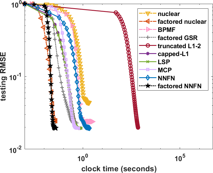
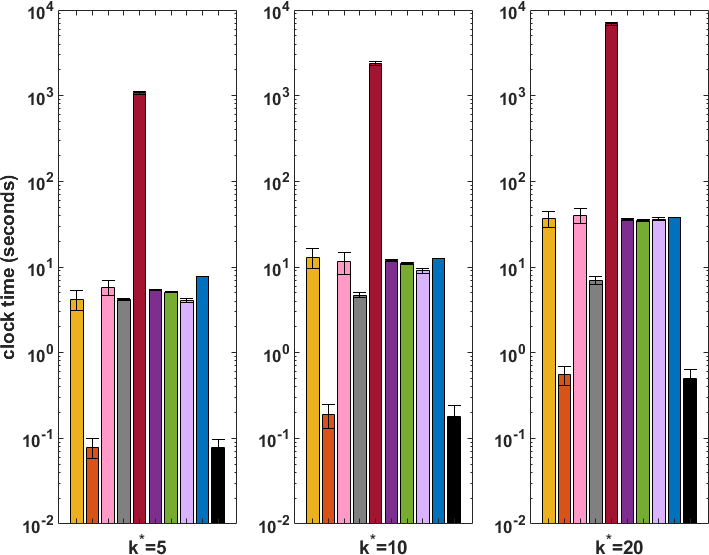
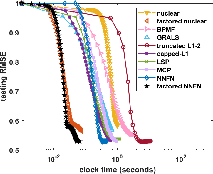
Table 4 shows the results. As can be seen, nonconvex regularizers (including the proposed $r_{\text{NNFN}}$) consistently yield better recovery performance. Among the nonconvex regularizers, all of them yield comparable errors. Additionally, we calculate the rank of recovered matrices and find that all methods (except the nuclear norm regularizer) can recover the true rank. As for speed, factored NNFN allows significantly faster optimization than NNFN, which validates the efficiency of using the factored form. Only factored nuclear norm regularizer is comparable to factored NNFN in speed (but it is much worse in terms of recovery performance), and both are orders of magnitudes faster than the others. Optimization with the truncated $\ell_{1\text{-}2}$ is exceptionally slow, which is due to the need of having two levels of DCA and ADMM iterations. The convergence of testing NMSE is put in Figure 2, which also shows factored NNFN always has the fastest convergence to the lowest NMSE.

(a) different noise variances.

(b) different ranks.

(c) different sparsity ratios.

Figure 3. Testing NMSE (first row) and clock time (second row) with different settings on the synthetic data ($m=1000$). The default setting is $k^{*}=5$, $\mathbf{E}\sim\mathcal{N}(0,0.1)$ and $s=6.91\%$. For each figure, we only vary one variable while keeping the others as the default setting.

6.2.2. Effects of Noise, Rank and Sparsity Ratio

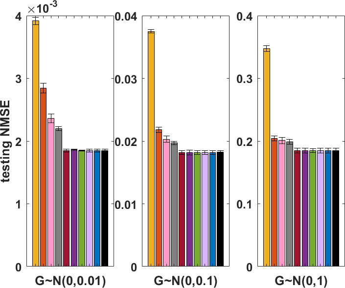
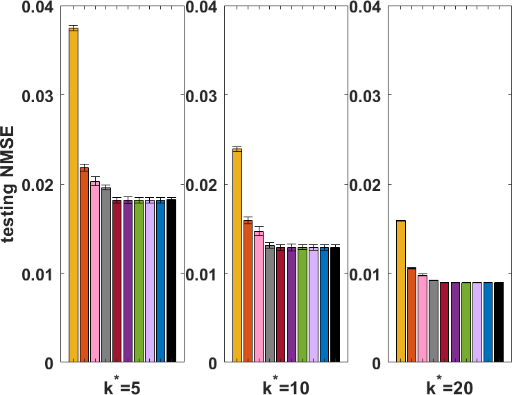
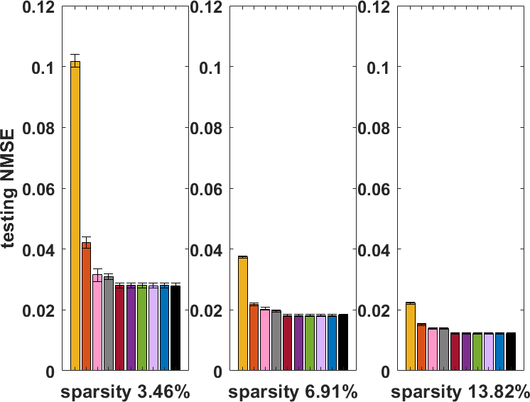
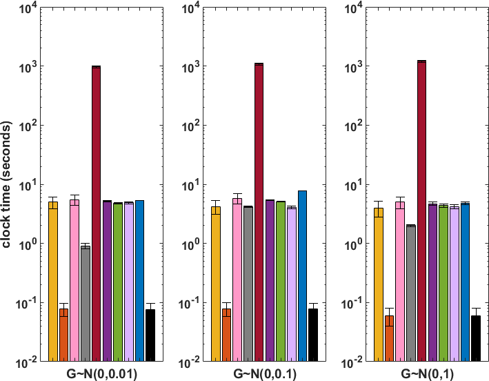
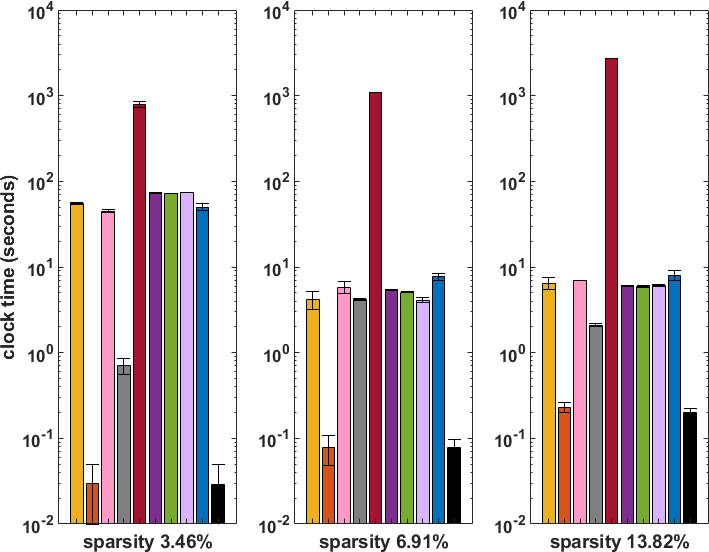
In this section, we vary (i) the variance of the Gaussian noise matrix $\mathbf{E}$ in the range $\{0.01,0.1,1\}$; (ii) the true rank $k^{*}$ of the data in $\{5,10,20\}$; and (iii) the sparsity ratio $s$ in $\{0.5,1,2\}\times(2mk^{*}\log(m)/m^{2})$. The experiment is performed on the synthetic data set, with $m=1000$. In each trial, we only vary one variable while keeping the others at default, i.e., $k^{*}=5$, $\mathbf{E}\sim\mathcal{N}(0,0.1)$ and $s=6.91\%$. Figure 3 shows the testing NMSE results and the timing results. As expected, a larger noise, smaller true rank, or sparser matrix lead to a harder matrix completion problem and subsequently higher NMSE’s. However, the relative performance ranking of the various methods remain the same, and nonconvex regularization always obtain a smaller NMSE. For time, although the exact timing results vary across different settings, consistent observation can be made: factored NNFN is consistently faster than the others.

Table 5. Performance on the recommendation data sets. Entries marked as “-” mean that the corresponding methods cannot complete in three hours. The best and comparable results (according to the pairwise t-test with 95% confidence) are highlighted in bold.

	MovieLens-1M		MovieLens-10M		Yahoo
	testing RMSE	time (s)	testing RMSE	time (s)	testing RMSE	time (s)
nuclear	0.820$\pm$0.002	118.7$\pm$19.2	0.807$\pm$0.001	821.2$\pm$27.7	0.721$\pm$0.001	1133.1$\pm$58.3
factored nuclear	0.810$\pm$0.001	0.6$\pm$0.1	0.795$\pm$0.001	41.8$\pm$7.3	0.710$\pm$0.008	533.9$\pm$25.7
BPMF	0.807$\pm$0.001	215.3$\pm$29.4	0.791$\pm$0.001	819.6$\pm$30.8	0.707$\pm$0.003	1433.5$\pm$89.2
factored GSR	0.805$\pm$0.001	14.2$\pm$1.5	-	-	-	-
truncated $\ell_{1-2}$	0.797$\pm$0.001	6068.4$\pm$172.0	-	-	-	-
capped-$\ell_{1}$	0.800$\pm$0.001	147.9$\pm$23.3	0.787$\pm$0.001	812.3$\pm$29.7	0.658$\pm$0.001	1296.8$\pm$67.3
LSP	0.799$\pm$0.001	149.2$\pm$23.5	0.787$\pm$0.001	850.8$\pm$31.1	0.656$\pm$0.001	1078.0$\pm$69.0
MCP	0.801$\pm$0.001	151.4$\pm$23.9	0.787$\pm$0.001	849.8$\pm$31.5	0.678$\pm$0.001	1108.3$\pm$41.4
NNFN	0.797$\pm$0.001	134.2$\pm$19.6	0.782$\pm$0.001	834.5$\pm$29.2	0.652$\pm$0.001	1209.7$\pm$61.2
factored NNFN	0.797$\pm$0.001	0.5$\pm$0.1	0.782$\pm$0.001	40.0$\pm$5.5	0.652$\pm$0.001	522.5$\pm$21.9

(a) MovieLens-1M.

(b) MovieLens-10M.

(c) Yahoo.

Figure 4. Testing RMSE versus clock time on recommendation data.

Table 6. Performance on the climate data sets. The best and comparable results (according to the pairwise t-test with 95% confidence) are highlighted in bold.

	GAS				USHCN
	$\textit{CO}_{2}$		$\textit{H}_{2}$		temperature		precipitation
	testing RMSE	time (s)	testing RMSE	time (s)	testing RMSE	time (s)	testing RMSE	time (s)
nuclear	0.584$\pm$0.005	1.0$\pm$0.1	0.593$\pm$0.006	0.8$\pm$0.1	0.480$\pm$0.014	108.5$\pm$4.1	0.828$\pm$0.020	84.9$\pm$11.2
factored nuclear	0.565$\pm$0.006	0.05$\pm$0.02	0.574$\pm$0.005	0.06$\pm$0.03	0.483$\pm$0.016	6.0$\pm$1.6	0.823$\pm$0.018	13.7$\pm$1.7
BPMF	0.552$\pm$0.005	3.2$\pm$0.3	0.554$\pm$0.005	3.4$\pm$0.4	0.464$\pm$0.012	148.1$\pm$7.7	0.819$\pm$0.015	125.1$\pm$8.1
GRALS	0.565$\pm$0.006	0.7$\pm$0.1	0.578$\pm$0.005	0.4$\pm$0.1	0.498$\pm$0.015	37.2$\pm$1.9	0.818$\pm$0.016	49.6$\pm$2.8
truncated $\ell_{1-2}$	0.530$\pm$0.007	11.0$\pm$1.2	0.531$\pm$0.005	7.3$\pm$1.8	0.444$\pm$0.013	573.9$\pm$18.1	0.806$\pm$0.014	318.5$\pm$9.7
capped-$\ell_{1}$	0.533$\pm$0.003	0.6$\pm$0.1	0.531$\pm$0.005	0.7$\pm$0.2	0.450$\pm$0.014	108.5$\pm$10.5	0.806$\pm$0.014	87.2$\pm$6.2
LSP	0.537$\pm$0.008	1.2$\pm$0.1	0.540$\pm$0.007	1.3$\pm$0.2	0.448$\pm$0.010	133.3$\pm$7.7	0.806$\pm$0.014	105.8$\pm$7.4
MCP	0.530$\pm$0.008	1.0$\pm$0.1	0.534$\pm$0.006	0.5$\pm$0.1	0.444$\pm$0.013	92.5$\pm$6.1	0.806$\pm$0.014	85.2$\pm$7.3
NNFN	0.530$\pm$0.008	0.4$\pm$0.1	0.531$\pm$0.005	0.5$\pm$0.1	0.444$\pm$0.012	57.1$\pm$3.3	0.806$\pm$0.014	66.4$\pm$5.1
factored NNFN	0.530$\pm$0.006	0.05$\pm$0.01	0.531$\pm$0.005	0.05$\pm$0.02	0.444$\pm$0.012	5.9$\pm$1.4	0.806$\pm$0.015	13.5$\pm$1.9

(a) GAS-$\textit{CO}_{2}$.

(b) GAS-$\textit{H}_{2}$.

(c) USHCN-temperature.

(d) USHCN-precipitation.

Figure 5. Testing RMSE versus clock time on climate data.

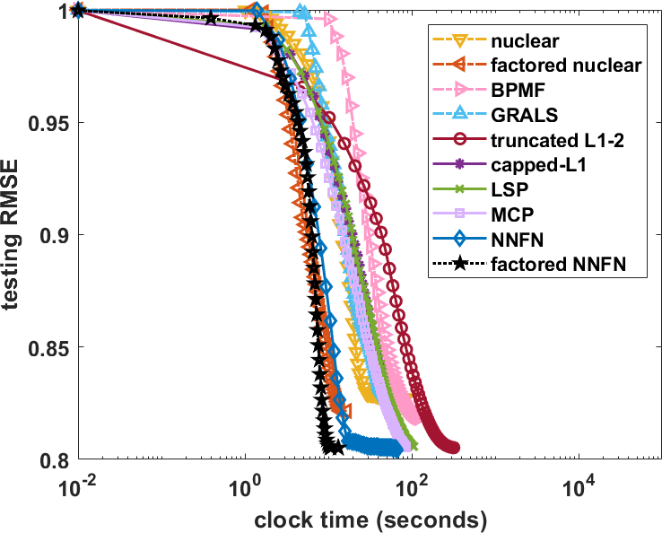
6.3. Recommendation Data

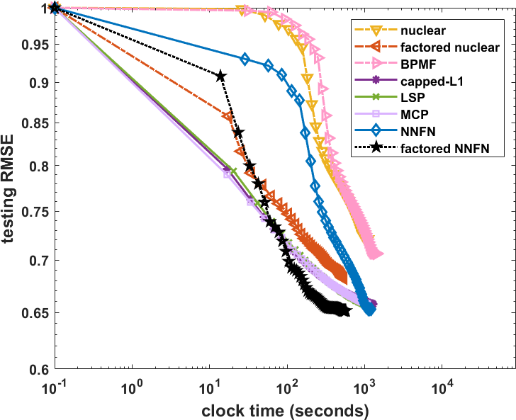
In this section, experiments are performed on the popularly used benchmark recommendation data sets: MovieLens-1M data set (Harper and Konstan, 2015) (of size $6,040\times 3,449$), MovieLens-10M data set (Harper and Konstan, 2015) (of size $69,878\times 10,677$) and Yahoo (Koren et al., 2009) data set (of size $249,012\times 296,111$). We uniformly sample 50% of the ratings as observed for training, 25% for validation (hyperparameter tuning) and the rest for testing. Optimization with the truncated $\ell_{1\text{-}2}$ cannot converge in three hours on MovieLens-10M and Yahoo, while Factored GSR runs out of memory on MovieLens-10M and Yahoo as it requires full matrices. Thus, their results are not reported.

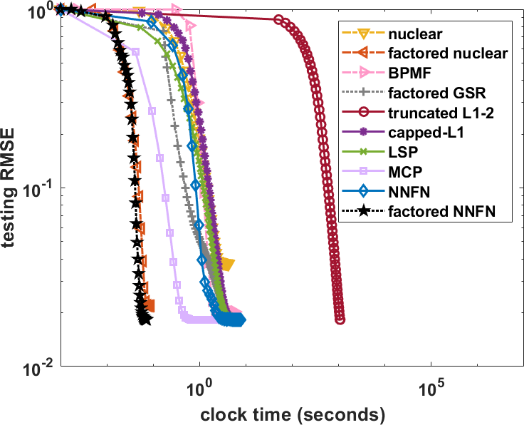
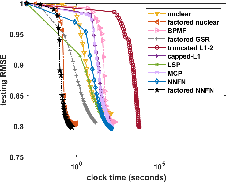
Table 5 shows the results. As can be seen, nonconvex regularizers obtain the best recovery performance than the other methods. Among them, factored NNFN is again the fastest. Figure 4 shows convergence of the testing RMSE. Consistent observation can be made, factored NNFN always obtains the best performance while being the fastest.

6.4. Climate Data

Additionally, we evaluated the proposed method on climate record data sets. The GAS and USHCN data sets from (Bahadori et al., 2014) are used. GAS contains monthly observations for the green gas components from January 1990 to December 2001, of which we use $\textit{CO}_{2}$ and $\textit{H}_{2}$. USHCN contains monthly temperature and precipitation readings from January 1919 to November 2019. For these two data sets, some rows (which correspond to locations) of the observed matrix are completely missing. The task is to predict climate observations for locations that do not have any records. Following (Bahadori et al., 2014), we normalize the data to zero mean and unit variance, then randomly sample 10% of the locations for training, another 10% for validation, and the rest for testing. To allow generalization to these completely unknown locations, we follow (Bahadori et al., 2014) and add a graph Laplacian regularizer to (1). Specifically, the $m$ locations are represented as nodes on a graph. The affinity matrix $\mathbf{A}=[A_{ij}]\in\mathbb{R}^{m\times m}$, which contains pairwise node similarities, is computed as $A_{ij}=\exp(-2b(i,j))$, where $b(i,j)$ is the Haversine distance between locations $i$ and $j$. The graph Laplacian regularizer is then defined as $a(\mathbf{X})=\text{tr}(\mathbf{X}^{\top}(\mathbf{D}-\mathbf{A})\mathbf{X})$, where $D_{ii}=\sum_{j}A_{ij}$. For the factored models (factored nuclear norm, BPMF and factored NNFN), we write $a(\mathbf{X})$ as $a(\mathbf{W}\mathbf{H}^{\top})$. Additionally, we compare with graph regularized alternating least squares (GRALS) (Rao et al., 2015), which optimizes for factored nuclear norm with $a(\mathbf{W})$.

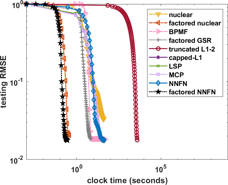
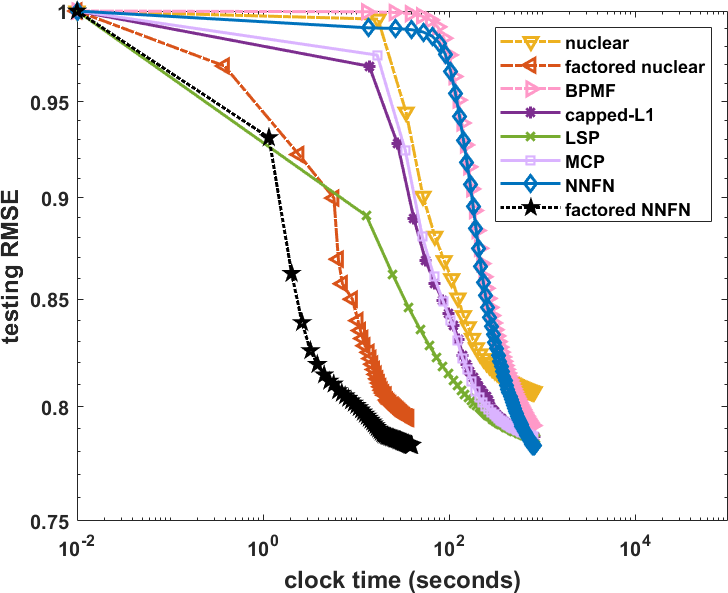
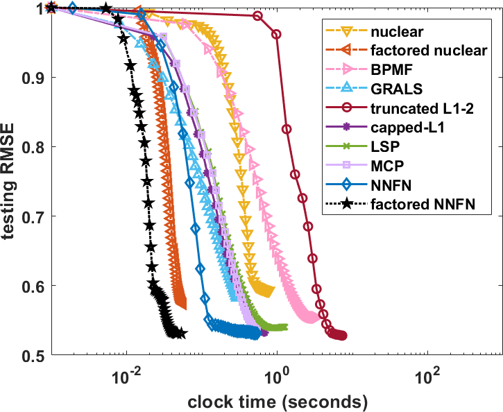
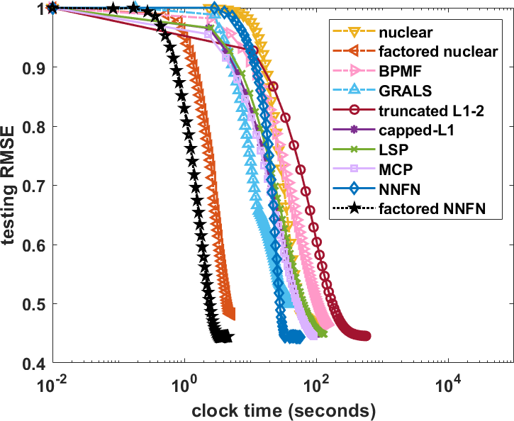
Results are shown in Table 6. They are consistent with the observations in the previous experiments. In terms of recovery performance, all the nonconvex regularizers (including NNFN and factored NNFN) have comparable performance and obtain the lowest testing RMSE. In terms of speed, factored NNFN and factored nuclear norm are again the fastest, and this speed advantage is particularly apparent on the larger USHCN data set. Figure 5 shows the convergence of RMSE. As shown, nonconvex regularizers generally obtain better testing RMSEs. Among them, factored NNFN is the fastest in convergence. This again validates the efficiency and effectiveness of factored NNFN.

7. Conclusion

We propose a scalable, adaptive and sound nonconvex regularizer for low-rank matrix learning. This regularizer can adaptively penalize singular values as common nonconvex regularizers. Further, we discover that learning with its factored form can be optimized by general solvers such as gradient-based method. We provide theoretical analysis for recovery and convergence guarantee. Extensive experiments on matrix completion problem show that the proposed algorithm achieves state-of-the-art recovery performance, while being the fastest among existing low-rank convex / nonconvex regularization and factored regularization methods. In sum, the proposed method can be useful to solve many large-scale matrix learning problems in the real world.

Appendix A Proof

A.1. Proposition 1

Lemma 1.

When Let $r(\mathbf{X})$ be a nonconvex low-rank regularizer of the form (4), and $\hat{r}(\alpha)$ is defined as in Table 5. As analyzed in (Lu et al., 2015b; Yao et al., 2019), $\hat{r}$ is a nonlinear, concave and non-decreasing function for $\alpha\geq 0$ with $\hat{r}(0)=0$, and

(12) $$p=\arg\min_{x}\frac{1}{2}(x-z)^{2}+\lambda\hat{r}(|x|).$$

Then, when $z\geq 0$, we have

• $0\leq p\leq z$,

• $z_{1}-p(z_{1})\leq z_{2}-p_{2}$ for $z_{1}\geq z_{2}$.

Proof.

The first point: Obvious, when $z\geq 0$, $p\geq 0$. Next, we prove $p\leq z$ by contradiction. Assume that $p>z$. Then as $\hat{r}$ is non-decreasing, we have $\hat{r}(|p|)\geq\hat{r}(|z|)$. Therefore we get

$$\frac{1}{2}(p-z)^{2}+\lambda\hat{r}(|z^{\prime}|)>\frac{1}{2}(z-z)^{2}+\lambda\hat{r}(|z|),$$

which leads to a contradiction that $p$ is the minimum solution found by optimizing (12). Thus, $p\leq z$.

The second point: The optimal of (12) $p$ satisfies

(13) $$p-z+\lambda\partial\hat{r}(p)=0.$$

As $\hat{r}$ is concave, for $z_{1}\geq z_{2}$, we have

(14) $$\partial\hat{r}(p_{1})\leq\partial\hat{r}(p_{2}).$$

Combining (14) and (13), we get $z_{1}-p_{1}\leq z_{2}-p_{2}$, and the second point is proved. ∎

Now, we can prove Proposition 1.

Proof.

Let the SVD of $\mathbf{Z}$ be $\bar{\mathbf{U}}\text{Diag}({\bm{\sigma}}(\mathbf{Z}))\bar{\mathbf{V}}^{\top}$. From Theorem 1 in (Lu et al., 2015b), we have $\bar{\mathbf{X}}\equiv\text{prox}_{\lambda r}(\mathbf{Z})=\bar{\mathbf{U}}\text{Diag}(\tilde{\bm{\sigma}})\bar{\mathbf{V}}^{\top}$, where $\tilde{\sigma}_{i}=\text{prox}_{\lambda\hat{r}}({\sigma}_{i}(\mathbf{Z}))$. Then, as every singular value $\sigma_{i}(\mathbf{Z})$ is nonnegative, by Lemma 1, we get the conclusion. Note that since $\hat{r}$ is not linear, thus the strict inequality in $\sigma_{i}(\mathbf{Z})-\tilde{\sigma}_{i}\leq{\sigma}_{i+1}(\mathbf{Z})-\tilde{\sigma}_{i+1}$ holds at least for one $i$. ∎

A.2. Proposition 2

Proof.

Let $\mathbf{X}=\mathbf{U}\text{Diag}(\tilde{\bm{\sigma}})\mathbf{V}^{\top}$ and $\mathbf{Z}=\bar{\mathbf{U}}\text{Diag}(\bm{\sigma}(\mathbf{Z}))\bar{\mathbf{V}}^{\top}$ be the SVD decomposition of $\mathbf{X}$ and $\mathbf{Z}$. By simple expansion, we have

$$\frac{1}{2}\|\mathbf{X}-\mathbf{Z}\|_{F}^{2}+\lambda r_{\text{NNFN}}(\mathbf{X})$$

$$=\frac{1}{2}\text{tr}(\mathbf{X}^{\top}\mathbf{X}+\mathbf{Z}^{\top}\mathbf{Z}-2\mathbf{X}^{\top}\mathbf{Z})+\lambda(\|\mathbf{X}\|_{*}-\theta\|\mathbf{X}\|_{F})$$

$$=\frac{1}{2}(\|\tilde{\bm{\sigma}}\|_{2}^{2}+\|\bm{\sigma}(\mathbf{Z})\|_{2}^{2})-\text{tr}(\mathbf{X}^{\top}\mathbf{Z})+\lambda\|\tilde{\bm{\sigma}}\|_{1}-\lambda\theta\|\tilde{\bm{\sigma}}\|_{2}.$$

Recall that $\text{tr}(\mathbf{X}^{\top}\mathbf{Z})\leq\tilde{\bm{\sigma}}^{\top}\bm{\sigma}(\mathbf{Z})$ achieves its equality at $\mathbf{U}=\bar{\mathbf{U}},\mathbf{V}=\bar{\mathbf{V}}$ (Jennings and McKeown, 1992). Then solving (7) can be instead computed by solving $\tilde{\bm{\sigma}}$ as

(15) $$\arg\min_{\tilde{\bm{\sigma}}} \frac{1}{2}\|\tilde{\bm{\sigma}}-\bm{\sigma}(\mathbf{Z})\|_{2}^{2}+\lambda(\|\tilde{\bm{\sigma}}\|_{1}-\theta\|\tilde{\bm{\sigma}}\|_{2})$$

s.t. $$\tilde{\sigma}_{1}\geq\tilde{\sigma}_{2}\geq\dots\geq\tilde{\sigma}_{m}\geq 0.$$

It can be solved by proximal operator as $\tilde{\bm{\sigma}}=\text{prox}_{\lambda\|\cdot\|_{1\text{-}2}}(\bm{\sigma}(\mathbf{Z}))$. The constraint in (15) is naturally satisfied. As $\sigma_{i}(\mathbf{Z})\geq 0$ and $\sigma_{i}(\mathbf{Z})\geq\sigma_{i+1}(\mathbf{Z})$ $\forall i$, we must have $\tilde{\sigma}_{i}\geq 0$ and $\tilde{\sigma}_{i}\geq\tilde{\sigma}_{i+1}$ $\forall i$. Otherwise, we can always swap the sign or value of $\tilde{\sigma}_{i}$ and $\tilde{\sigma}_{i+1}$ and obtain a smaller objective of (15). ∎

A.3. Corollary 3

Proof.

Let $\mathbf{X}=\mathbf{U}\text{Diag}(\tilde{\bm{\sigma}})\mathbf{V}^{\top}$ where $\tilde{\bm{\sigma}}=\text{prox}_{\lambda\|\cdot\|_{1\text{-}2}}(\bm{\sigma}(\mathbf{Z}))$. Now we prove that

• shrinkage: ${\sigma}_{i}(\mathbf{Z})\geq\tilde{\sigma}_{i}$,

• adaptivity: $\sigma_{i}(\mathbf{Z})-\tilde{\sigma}_{i}\leq{\sigma}_{i+1}(\mathbf{Z})-\tilde{\sigma}_{i+1}$, where the strict inequality holds at least for one $i$.

The first point: From Proposition 2, we can see the optimization problem on matrix (7) can be transformed to an optimization problem on singular values (15). As shown in Proposition 2, for $\tilde{\bm{\sigma}}=\text{prox}_{\lambda\|\cdot\|_{1\text{-}2}}(\bm{\sigma}(\mathbf{Z}))$, we have $\sigma_{i}(\mathbf{Z})\geq\tilde{\sigma}_{i}\geq 0$.

The second point: The optimal of (15) satisfies

$$\tilde{\bm{\sigma}}-\bm{\sigma}(\mathbf{Z})+\lambda-\lambda\frac{\tilde{\bm{\sigma}}}{\|\tilde{\bm{\sigma}}\|_{2}}=0.$$

As $\sigma_{i}(\mathbf{Z})\geq\tilde{\sigma}_{i}\geq 0$, we have

$$\sigma_{i}(\mathbf{Z})-\tilde{\sigma}_{i}=\lambda-\lambda\frac{\tilde{\sigma}_{i}}{\|\tilde{\bm{\sigma}}\|_{2}}\geq 0.$$

Then as $\tilde{\sigma}_{i}\geq\tilde{\sigma}_{i+1}$, we have

$$\lambda-\lambda\frac{\tilde{\sigma}_{i}}{\|\tilde{\bm{\sigma}}\|_{2}}\leq\lambda-\lambda\frac{\tilde{\sigma}_{i+1}}{\|\tilde{\bm{\sigma}}\|_{2}},$$

and correspondingly $\sigma_{i}(\mathbf{Z})-\tilde{\sigma}_{i}\leq{\sigma}_{i+1}(\mathbf{Z})-\tilde{\sigma}_{i+1}$. The inequality holds only when $\sigma_{i}(\mathbf{Z})\neq\sigma_{i+1}(\mathbf{Z})$. ∎

A.4. Theorem 2

Proof.

The regularized and constrained low-rank matrix completion problem obtain equivalent solutions (Boyd et al., 2004). Here, we prove for the constrained problem, but the conclusion applies for both forms.

Assume sequence $\{\mathbf{X}^{t}\}$ with $f(\mathbf{X}^{t+1})<f(\mathbf{X}^{t})$ and each $\mathbf{X}^{t}$ is the iterate obtained by optimizing the following two equivalent constrained formulations of (8): (i) $\mathbf{X}^{t}$ is the iterate of optimizing $\min\nolimits_{\mathbf{X}}f(\mathbf{X})\!\;\!\;\text{s.t.}\;\!\;\!r_{\text{NNFN}}(\mathbf{X})\!\leq\!\beta^{\prime}$, where $\beta^{\prime}\geq 0$ is a hyperparameter. or (ii) $\mathbf{X}^{t}\!=\!\mathbf{W}^{t}(\mathbf{H}^{t})^{\top}$ is the iterate of optimizing $\min\nolimits_{\mathbf{W},\mathbf{H}}f(\mathbf{W}\mathbf{H}^{\top})$ $\!\;\!\;\text{s.t.}\;\!\;\!\frac{1}{2}(\|\mathbf{W}\|_{F}^{2}\!+\!\|\mathbf{H}\|_{F}^{2})\!-\!\|\mathbf{W}\mathbf{H}^{\top}\|_{F}\!\leq\!\beta^{\prime}$, where $\beta^{\prime}\geq 0$ is a hyperparameter. These sequences can be obtained by optimizing the two constrained problems via projected gradient descent which guarantees sufficient decrease in $f$ (Boyd et al., 2004; Nocedal and Wright, 2006).

Obviously, the optimal $\mathbf{X}^{*}$ satisfies $\mathbf{b}-\mathcal{A}(\mathbf{X}^{*})=\mathbf{e}$ and hence $f(\mathbf{X}^{*})=\frac{1}{2}\|\mathcal{A}(\mathbf{X}^{*})-\mathbf{b}\|_{2}^{2}=\frac{\|\mathbf{e}\|_{2}^{2}}{2}$. Thus $\mathbf{X}^{t}$ obtained at the $t$th iteration satisfies $f(\mathbf{X}^{t})\geq\frac{c_{1}^{2}\|\mathbf{e}\|_{2}^{2}}{2}\geq\frac{\|\mathbf{e}\|_{2}^{2}}{2}$ for constant $c_{1}$ whose absolute value is larger than 1. By choosing the dimension $k$ of $\mathbf{W}\in\mathbb{R}^{m\times k}$, one can let $\mathbf{X}^{t}\leq k^{*}$, where $k^{*}$ is the true rank of the optimal matrix $\mathbf{X}^{*}$.

We can derive

$$\|\mathcal{A}(\mathbf{X}^{*}-\mathbf{X}^{t})\|_{2}^{2} \leq\|(\mathbf{b}-\mathcal{A}(\mathbf{X}^{t}))-\mathbf{e}\|_{2}^{2},$$

$$\leq 2\left(f(\mathbf{X}^{t})-\mathbf{e}^{\top}(\mathbf{b}-\mathcal{A}(\mathbf{X}^{t}))+\frac{\|\mathbf{e}\|^{2}}{2}\right),$$

$$\leq 2\left(f(\mathbf{X}^{t})+\frac{2}{c_{1}}f(\mathbf{X}^{t})+\frac{1}{c_{1}^{2}}f(\mathbf{X}^{t})\right),$$

(16) $$\leq 2\left(1+\frac{1}{c_{1}}\right)^{2}f(\mathbf{X}^{t})$$

Now, we are ready to bound the difference between this $\mathbf{X}^{t}$ and the optimal $\mathbf{X}^{*}$.

(17) $$\|\mathbf{X}^{t}-\mathbf{X}^{*}\|_{F}^{2} \leq\frac{1}{1-\delta_{2k^{*}}}\|\mathcal{A}(\mathbf{X}^{t}-\mathbf{X}^{*})\|_{2}^{2}$$

(18) $$\leq\frac{2}{1-\delta_{2k^{*}}}\left(1+\frac{1}{c_{1}}\right)^{2}f(\mathbf{X}^{t})$$

(19) $$\leq\frac{1}{1-\delta_{2k^{*}}}\left(1+\frac{1}{c_{1}}\right)^{2}(c_{1}^{2}+\epsilon)\|\mathbf{e}\|^{2}_{2}$$

$$=\frac{(c_{1}+1)^{2}(c_{1}^{2}+\epsilon)\|\mathbf{e}\|^{2}_{2}}{c_{1}^{2}(1-\delta_{2k^{*}})},$$

where the isometry constant is $\delta_{2k^{*}}$ as $\mathbf{X}^{t}-\mathbf{X}^{*}$ is a matrix of rank at most $2k^{*}$, (17) is derived from RIP, (18) comes from (16), and (19) is obtained as one can choose a small constant $\epsilon$ such that $\frac{(c_{1}^{2}+\epsilon)\|\mathbf{e}\|_{2}^{2}}{2}\geq f(\mathbf{X}^{t})\geq\frac{c_{1}^{2}\|\mathbf{e}\|_{2}^{2}}{2}$.

∎

A.5. Theorem 3

Proof.

For smooth functions, gradient descent can obtain sufficient decrease as shown in the following Proposition.

Proposition 2 ((Nocedal and Wright, 2006)).

A differentiable function $h$ with $L$-Lipschitz continuous gradient, i.e., $\|\nabla_{x}h(x^{t})-\nabla_{x}h(x^{t+1})\|_{2}\leq L\|x^{t}-x^{t+1}\|_{2}$, satisfies the following inequality,

$$h(x^{t})-h(x^{t+1})\geq\frac{1}{2L}\|\nabla_{x}h(x^{t})\|_{F}^{2}.$$

Moreover, when $h$ is bounded from below, i.e., $\inf h(x)>-\infty$ and $\lim_{\|x\|_{2}\rightarrow\infty}h(x)=\infty$, optimizing $h$ by gradient descent is guaranteed to converge.

Since $\mathbf{W}_{t}\mathbf{H}_{t}^{\top}\not=\mathbf{0}$, $F(\mathbf{W},\mathbf{H})$ is smooth. As gradient descent is used, we then have

$$F(\mathbf{W}^{t},\mathbf{H}^{t})-F(\mathbf{W}^{t+1},\mathbf{H}^{t+1})$$

$$\geq\frac{\eta}{2}\|\nabla_{\mathbf{W}}F(\mathbf{W}^{t},\mathbf{H}^{t})\|_{F}^{2}+\frac{\eta}{2}\|\nabla_{\mathbf{H}}F(\mathbf{W}^{t},\mathbf{H}^{t})\|_{F}^{2}.$$

At the $(T+1)$th iteration, the difference between $F(\mathbf{W}^{1},\mathbf{H}^{1})$ and $F(\mathbf{W}^{T+1},\mathbf{H}^{T+1})$ is calculated as

$$F(\mathbf{W}^{1},\mathbf{H}^{1})\!-\!F(\mathbf{W}^{T+1},\mathbf{H}^{T+1})$$

(20) $$\geq\sum_{t=1}^{T}\frac{\eta}{2}\|\nabla_{\mathbf{W}}F(\mathbf{W}^{t},\mathbf{H}^{t})\|_{F}^{2}\!+\!\frac{\eta}{2}\|\nabla_{\mathbf{H}}F(\mathbf{W}^{t},\mathbf{H}^{t})\|_{F}^{2}.\!$$

As assumed, $\lim\nolimits_{\|\mathbf{W}\|_{F}\rightarrow\infty}F(\mathbf{W},\cdot)=\infty$, $\lim\nolimits_{\|\mathbf{H}\|_{F}\rightarrow\infty}F(\cdot,\mathbf{H})=\infty$. Thus $\infty>F(\mathbf{W}^{1},\mathbf{H}^{1})-F(\mathbf{W}^{T+1},\mathbf{H}^{T+1})\geq c$, where $c$ is a finite constant. Combining this with (20), when $T\rightarrow\infty$, we see that a sum of infinite sequence is smaller than a finite constant. This means the sequence $\{\mathbf{W}^{t},\mathbf{H}^{t}\}$ has limit points. Let $\{\bar{\mathbf{W}},\bar{\mathbf{H}}\}$ be a limit point, we must have

$$\nabla_{\mathbf{W}}F(\bar{\mathbf{W}},\bar{\mathbf{H}})=0\text{\;and\;}\nabla_{\mathbf{H}}F(\bar{\mathbf{W}},\bar{\mathbf{H}})=0.$$

By definition, this shows $\{\bar{\mathbf{W}},\bar{\mathbf{H}}\}$ is a critical point of (8).

Next, we proceed to prove that $\bar{\mathbf{X}}=\bar{\mathbf{W}}\bar{\mathbf{H}}^{\top}$ is the the critical point of (1) with $r(\mathbf{X})=r_{\text{NNFN}}(\mathbf{X})$.

As shown in (Srebro et al., 2005), the nuclear norm can be reformulated in terms of factorized matrices. Then we have

$$\min_{\mathbf{W},\mathbf{H}} f(\mathbf{W}\mathbf{H}^{\top})-\lambda\|\mathbf{W}\mathbf{H}^{\top}\|_{F}+\nicefrac{{\lambda}}{{2}}(\|\mathbf{W}\|_{F}^{2}+\|\mathbf{H}\|_{F}^{2})$$

$$\geq \min_{\mathbf{X}}f(\mathbf{X})-\lambda\|\mathbf{X}\|_{F}+\min_{\mathbf{X}=\mathbf{W}\mathbf{H}^{\top}}\nicefrac{{\lambda}}{{2}}(\|\mathbf{W}\|_{F}^{2}+\|\mathbf{H}\|_{F}^{2})$$

$$\geq \min_{\mathbf{X}}f(\mathbf{X})-\lambda\|\mathbf{X}\|_{F}+\lambda\|\mathbf{X}\|_{*}.$$

Thus, if $(\bar{\mathbf{W}},\bar{\mathbf{H}})$ is a critical point of (8), then $\bar{\mathbf{X}}=\bar{\mathbf{W}}(\bar{\mathbf{H}})^{\top}$ is also critical point of (1) with $r(\mathbf{X})=r_{\text{NNFN}}(\mathbf{X})$. ∎

References

- (1)
- Bahadori et al. (2014) Mohammad Taha Bahadori, Qi Rose Yu, and Yan Liu. 2014. Fast multivariate spatio-temporal analysis via low rank tensor learning. In Advances in Neural Information Processing Systems. 3491–3499.
- Bolte et al. (2014) Jérôme Bolte, Shoham Sabach, and Marc Teboulle. 2014. Proximal alternating linearized minimization for nonconvex and nonsmooth problems. Mathematical Programming 146, 1-2 (2014), 459–494.
- Boumal and Absil (2015) Nicolas Boumal and P-A Absil. 2015. Low-rank matrix completion via preconditioned optimization on the Grassmann manifold. Linear Algebra Appl. 475 (2015), 200–239.
- Boyd et al. (2004) Stephen Boyd, Stephen P Boyd, and Lieven Vandenberghe. 2004. Convex Optimization. Cambridge University Press.
- Boyd et al. (2011) Stephen Boyd, Neal Parikh, and Eric Chu. 2011. Distributed optimization and statistical learning via the alternating direction method of multipliers. Foundations and Trends in Machine Learning 3, 1 (2011), 1–122.
- Cai et al. (2010) Jian-Feng Cai, Emmanuel J Candès, and Zuowei Shen. 2010. A singular value thresholding algorithm for matrix completion. SIAM Journal on Optimization 20, 4 (2010), 1956–1982.
- Candès and Recht (2009) Emmanuel J Candès and Benjamin Recht. 2009. Exact matrix completion via convex optimization. Foundations of Computational Mathematics 9, 6 (2009), 717–772.
- Candes and Tao (2005) Emmanuel J Candes and Terence Tao. 2005. Decoding by linear programming. IEEE Transactions on Information Theory 51, 12 (2005), 4203–4215.
- Candes et al. (2008) Emmanuel J Candes, Michael B Wakin, and Stephen P Boyd. 2008. Enhancing sparsity by reweighted minimization. Journal of Fourier Analysis and Applications 14, 5-6 (2008), 877–905.
- Chen et al. (2011) Jianhui Chen, Jiayu Zhou, and Jieping Ye. 2011. Integrating low-rank and group-sparse structures for robust multi-task learning. In International Conference on Knowledge Discovery and Data Mining. 42–50.
- Fan et al. (2019) Jicong Fan, Lijun Ding, Yudong Chen, and Madeleine Udell. 2019. Factor group-sparse regularization for efficient low-rank matrix recovery. In Advances in Neural Information Processing Systems. 5104–5114.
- Fazel (2002) Maryam Fazel. 2002. Matrix Rank Minimization with Applications. Ph.D. Dissertation. Stanford.
- Ge et al. (2016) Rong Ge, Jason D Lee, and Tengyu Ma. 2016. Matrix completion has no spurious local minimum. In Advances in Neural Information Processing Systems. 2973–2981.
- Gu et al. (2014) Shuhang Gu, Lei Zhang, Wangmeng Zuo, and Xiangchu Feng. 2014. Weighted nuclear norm minimization with application to image denoising. In Conference on Computer Vision and Pattern Recognition. 2862–2869.
- Gui et al. (2016) Huan Gui, Jiawei Han, and Quanquan Gu. 2016. Towards faster rates and oracle property for low-rank matrix estimation. In International Conference on Machine Learning. 2300–2309.
- Gunasekar et al. (2017) Suriya Gunasekar, Blake Woodworth, Srinadh Bhojanapalli, Behnam Neyshabur, and Nathan Srebro. 2017. Implicit regularization in matrix factorization. In Advances in Neural Information Processing Systems. 6151–6159.
- Harper and Konstan (2015) F Maxwell Harper and Joseph A Konstan. 2015. The movielens datasets: History and context. ACM Transactions on Interactive Intelligent Systems 5, 4 (2015), 1–19.
- Hastie et al. (2015) Trevor Hastie, Rahul Mazumder, Jason D Lee, and Reza Zadeh. 2015. Matrix completion and low-rank SVD via fast alternating least squares. Journal of Machine Learning Research 16, 1 (2015), 3367–3402.
- Hiriart-Urruty (1985) J-B Hiriart-Urruty. 1985. Generalized differentiability, duality and optimization for problems dealing with differences of convex functions. In Proceedings of the Symposium on Convexity and Duality in Optimization. 37–70.
- Hu et al. (2012) Yao Hu, Debing Zhang, Jieping Ye, Xuelong Li, and Xiaofei He. 2012. Fast and accurate matrix completion via truncated nuclear norm regularization. IEEE Transactions on Pattern Analysis and Machine Intelligence 35, 9 (2012), 2117–2130.
- Jennings and McKeown (1992) Alan Jennings and John J McKeown. 1992. Matrix Computation. John Wiley & Sons.
- Koren et al. (2009) Yehuda Koren, Robert Bell, and Chris Volinsky. 2009. Matrix factorization techniques for recommender systems. Computer 42, 8 (2009), 30–37.
- Li et al. (2018) Dongsheng Li, Chao Chen, Qin Lv, Hansu Gu, Tun Lu, Li Shang, Ning Gu, and Stephen M Chu. 2018. AdaError: An adaptive learning rate method for matrix approximation-based collaborative filtering. In The World Wide Web Conference. 741–751.
- Lou and Yan (2018) Yifei Lou and Ming Yan. 2018. Fast L1-L2 minimization via a proximal operator. Journal of Scientific Computing 74, 2 (2018), 767–785.
- Lu et al. (2015a) Canyi Lu, Jinhui Tang, Shuicheng Yan, and Zhouchen Lin. 2015a. Nonconvex nonsmooth low rank minimization via iteratively reweighted nuclear norm. IEEE Transactions on Image Processing 25, 2 (2015), 829–839.
- Lu et al. (2015b) Canyi Lu, Changbo Zhu, Chunyan Xu, Shuicheng Yan, and Zhouchen Lin. 2015b. Generalized singular value thresholding. In AAAI Conference on Artificial Intelligence. 1805–1811.
- Ma et al. (2017) Tian-Hui Ma, Yifei Lou, and Ting-Zhu Huang. 2017. Truncated models for sparse recovery and rank minimization. SIAM Journal on Imaging Sciences 10, 3 (2017), 1346–1380.
- Mazumder et al. (2020) Rahul Mazumder, Diego Saldana, and Haolei Weng. 2020. Matrix completion with nonconvex regularization: Spectral operators and scalable algorithms. Statistics and Computing (2020), 1–26.
- Mnih and Salakhutdinov (2008) Andriy Mnih and Russ R Salakhutdinov. 2008. Probabilistic matrix factorization. In Advances in Neural Information Processing Systems. 1257–1264.
- Nie et al. (2012) Feiping Nie, Heng Huang, and Chris Ding. 2012. Low-rank matrix recovery via efficient schatten p-norm minimization. In AAAI Conference on Artificial Intelligence.
- Nocedal and Wright (2006) Jorge Nocedal and Stephen Wright. 2006. Numerical Optimization. Springer Science & Business Media.
- Parikh and Boyd (2014) Neal Parikh and Stephen Boyd. 2014. Proximal algorithms. Foundations and Trends in Optimization 1, 3 (2014), 127–239.
- Pennington et al. (2014) Jeffrey Pennington, Richard Socher, and Christopher D Manning. 2014. Glove: Global vectors for word representation. In Conference on Empirical Methods in Natural Language Processing. 1532–1543.
- Rao et al. (2015) Nikhil Rao, Hsiang-Fu Yu, Pradeep Ravikumar, and Inderjit S Dhillon. 2015. Collaborative filtering with graph information: Consistency and scalable methods. In Advances in Neural Information Processing Systems. 2107–2115.
- Salakhutdinov and Mnih (2008) Ruslan Salakhutdinov and Andriy Mnih. 2008. Bayesian probabilistic matrix factorization using Markov chain Monte Carlo. In International Conference on Machine Learning. 880–887.
- Shang et al. (2016) Fanhua Shang, Yuanyuan Liu, and James Cheng. 2016. Tractable and scalable Schatten quasi-norm approximations for rank minimization. In Artificial Intelligence and Statistics. 620–629.
- Sharma and Karypis (2019) Mohit Sharma and George Karypis. 2019. Adaptive matrix completion for the users and the items in tail. In The World Wide Web Conference. 3223–3229.
- Shi et al. (2018) Tian Shi, Kyeongpil Kang, Jaegul Choo, and Chandan K Reddy. 2018. Short-text topic modeling via non-negative matrix factorization enriched with local word-context correlations. In The World Wide Web Conference. 1105–1114.
- Srebro et al. (2005) Nathan Srebro, Jason Rennie, and Tommi S Jaakkola. 2005. Maximum-margin matrix factorization. In Advances in Neural Information Processing Systems. 1329–1336.
- Tu et al. (2016) Stephen Tu, Ross Boczar, Max Simchowitz, Mahdi Soltanolkotabi, and Ben Recht. 2016. Low-rank solutions of linear matrix equations via procrustes flow. In International Conference on Machine Learning. 964–973.
- Vandereycken (2013) Bart Vandereycken. 2013. Low-rank matrix completion by Riemannian optimization. SIAM Journal on Optimization 23, 2 (2013), 1214–1236.
- Wang et al. (2017) Lingxiao Wang, Xiao Zhang, and Quanquan Gu. 2017. A unified computational and statistical framework for nonconvex low-rank matrix estimation. In Artificial Intelligence and Statistics. 981–990.
- Wen et al. (2012) Zaiwen Wen, Wotao Yin, and Yin Zhang. 2012. Solving a low-rank factorization model for matrix completion by a nonlinear successive over-relaxation algorithm. Mathematical Programming Computation 4, 4 (2012), 333–361.
- Yao et al. (2019) Quanming Yao, James T Kwok, Taifeng Wang, and Tie-Yan Liu. 2019. Large-scale low-rank matrix learning with nonconvex regularizers. IEEE Transactions on Pattern Analysis and Machine Intelligence 41, 11 (2019), 2628–2643.
- Zhang (2010a) Cun-Hui Zhang. 2010a. Nearly unbiased variable selection under minimax concave penalty. The Annals of Statistics 38, 2 (2010), 894–942.
- Zhang (2010b) Tong Zhang. 2010b. Analysis of multi-stage convex relaxation for sparse regularization. Journal of Machine Learning Research 11, Mar (2010), 1081–1107.