NT@UW-20-06
Discovery vs. Precision in Nuclear Physics- A Tale of Three Scales

Abstract

At least three length scales are important in gaining a complete understanding of the physics of nuclei. These are the radius of the nucleus, the average inter-nucleon separation distance, and the size of the nucleon. The connections between the different scales are examined by using examples that demonstrate the direct connection between short-distance and high momentum transfer physics and also that significant high momentum content of wave functions is inevitable. The nuclear size is connected via the independent-pair approximation to the nucleon-nucleon separation distance, and this distance is connected via the concept of virtuality to the EMC effect. An explanation of the latter is presented in terms of light-front holographic wave functions of QCD. The net result is that the three scales are closely related, so that a narrow focus on any given specific range of scales may prevent an understanding of the fundamental origins of nuclear properties. It is also determined that, under certain suitable conditions, experiments are able to measure the momentum dependence of wave functions.

I Introduction

In studying atomic nuclei one encounters three different length scales: the nuclear radius $R_{A}(\approx 5$ fm for a heavy nucleus), the average separation between nucleons at the centers of nuclei $d\approx 1.7$ fm, and the nucleon radius, $r_{N}\approx 0.84$ fm. The pion Compton wave length, $1/m_{\pi}=$ 1.4 fm is close to $d$, so is not a separate scale. The correlation length associated with the Fermi momentum, $\approx\pi/k_{F}$ Bohr and Mottelson (1998) is also of the order of $d$.

The general modern trend of theorists is to focus on each length scale of a given subject using the techniques of effective field theory. The main idea (see e.g. Georgi (1993)) is: if there are parameters that are very large or very small compared to the physical quantities (with the same dimension) of interest, one may get a simpler approximate description of the physics by setting the small parameters to zero and the large parameters to infinity. Then the finite effects of the large parameters can be included as small perturbations about the simple approximate starting point.

This scale separation is a common technique (see e.g. Cohen (2019)) in which physics at large distances is assumed not to depend on physics at shorter distances. A famous example is the weak interaction in which the effects of $W$ and $Z$ boson exchanges can be treated as contact (zero-ranged) interactions at low energies. The general philosophy is that if one is working at a low mass scale $m$ one doesn’t need to consider dynamics at a mass scale $\Lambda\gg m$. Or in terms of distances: the long distance scale $1/m$ must be very much greater than the short distance scale $1/\Lambda$. In other words, there must be a large separation of scales for effective field theory techniques to be maximally efficient. In nuclear physics the scale separation is not very large–the values of relevant distances are not widely separated.

In using effective field theory, theorists concentrate on a given range of length scales. A typical procedure is to make robust calculations that enable firm predictions. These are then tested by experiments, and the results may confirm the theories or (more likely) lead to revision of the theories. Another scenario, in which experiment leads, is that an experiment discovers an unexpected phenomenon, such as the Rutherford’s discovery of the atomic nucleus or the SLAC-MIT discovery of quarks within the nucleon Bloom et al. (1969); Friedman and Kendall (1972).

The two approaches of the previous paragraph can be summarized as precision vs discovery. The effective field theory approach of working within a given scale is aptly suited for precision work. In contrast, discovery of new phenomena is not well treated by scale separation techniques because new phenomena are often related to discovering a new relevant scale.

I comment on the precision approach. Much current activity in precision nuclear structure calculations is based on using low energy, long length scale treatments. These began with interactions, known as $V_{{\rm low}\,k}$, that use renormalization group transformations that lower a cutoff in relative momentum to derive NN potentials with vanishing matrix elements for momenta above the cutoff. Such interactions show greatly enhanced convergence properties in nuclear few- and many-body systems for cutoffs of order $\Lambda=2\,\text{fm}^{-1}$ or lower Bogner et al. (2003a, b, 2001); Nogga et al. (2004); Bogner et al. (2005). Later calculations use renormalization group methods to soften interactions in nuclear systems. This extends the range of many computational methods and qualitatively improves their convergence patterns Bogner et al. (2010). The similarity renormalization group (SRG) Glazek and Wilson (1993); Szpigel and Perry (2000); Bogner et al. (2007a) does this by systematically evolving Hamiltonians via a continuous series of unitary transformations chosen to decouple the high- and low-energy matrix elements of a given interaction Jurgenson et al. (2008, 2009).

However, many conventional NN potentials, feature strong short-range repulsion Epelbaum et al. (2009). This is supported by some lattice gauge QCD calculations  Ishii et al. (2007); Aoki et al. (2010); Murano et al. (2011); Doi et al. (2016); Aoki et al. (2018, ). The repulsion causes bound states with very low energies (such as the deuteron) to have important contributions to the binding and other properties from high-momentum components.

In Ref. Benhar and Pandharipande (1993), the authors calculate cross sections for electron scattering from light nuclei. They conclude: “and thus the data confirm the existence of high-momentum components in the deuteron wave function”. The high-momentum components of the deuteron lead to inclusive electron-scattering cross section ratios with simple scaling properties Frankfurt et al. (1993). That reference finds significant “evidence for the dominance of short-range correlations in nuclei”. Ref. Bogner et al. (2007b) argued that the statement of Ref. Benhar and Pandharipande (1993) (and by implication that of Ref. Frankfurt et al. (1993)) is not correct because wave functions are not observables. Similarly Ref. Furnstahl and Hammer (2002) argued that nuclear momentum distributions are not observable. It is certainly true that wave functions are not observable quantities, but cross sections are observables.

There are prominent examples that momentum-space wave functions are closely related to cross sections. Showing that the cross section of the photo-electric effect in hydrogen is proportional to the square of the momentum-space ground-state wave function of hydrogen is a text-book problem Sakurai and Napolitano (2017); Gottfried et al. (2003). The modern version of the photo-electric effect is called Angle Resolved Photoemission Spectroscopy (ARPES) a technique that is well-known, see e.g. Ref. Damascelli et al. (2003), to yield information of about the momentum and energy states of electrons in materials. The statement that measurements of cross sections can be used to learn about wave functions violates no principles of quantum mechanics.

One of the purposes of this paper is to exemplify how the use of the impulse approximation simplifies the connection between cross sections and wave functions for nuclear processes at high momentum transfer. If the kinematics are correctly chosen the effects of various processes that are not directly related to wave functions can be minimized Schmidt et al. (2020), so that in effect measuring cross section measures important properties of wave functions. See Sects. IV, VI, and VII.

The principle concern of the present epistle is that current experiments involving nuclei cover all the three scales mentioned above. Deep inelastic scattering experiments on nuclei, involving squares of four momentum transfers ($Q^{2}$) between 10 and hundreds of GeV² have shown that the quark properties (quark distributions) of nucleons bound in nuclei are different than those of free nucleons. This phenomenon is known as the EMC effect; see e.g. the review Hen et al. (2017). The effect is not large, of order 10-15%, but is of fundamental interest because it involves the influence of nuclear properties on scales that resolve the nucleon size. But scales larger than the nucleon size are relevant because modifications of nucleon structure must be caused by interactions with nearby nucleons. Indeed, after the nucleon size, the next largest length is the inter-nucleon separation length, $d$. This is the scale associated with short range correlations between nucleons. Therefore the EMC effect is naturally connected with short range correlations between nucleons. But the inter-nucleon separation is not very much smaller than that of the nuclear size. This means that effects involving the entire nucleus cannot be disregarded. Such effects are known as mean-field effects in which each nucleon moves in the mean field provided by other nucleons. Understanding the EMC effect involves understanding physics at all three length scales.

Here is an outline of the remainder of this paper. Sect. II presents a short review of the modern technique of softening the nucleon-nucleon interactions to simplify calculations of low-energy nuclear properties. The consequence of this softening is the hardening of the leptonic interactions that probe the system. Sect. III is concerned with the largest of the three nuclear distance scales–the nuclear radius. This is followed by a discussion of the physics of the separation between two nucleons in bound states, Sec. IV. The consequent nuclear manifestations are discussed in Sect. V. This involves understanding the connection between the physics of short distances and high momentum. It is shown that the momentum dependence of wave functions can in principle be observed by measuring elastic form factors. Next, Sect. VI discusses the $(e,e^{\prime}p)$ reaction as a discovery mechanism for the physics of the two-nucleon separation distance. The concept of virtuality (the difference between the square of the four-momentum and the square of the mass) as a connection between the scale of the two-nucleon separation-distance and the nucleon size is introduced in Sec. VII. The connection between virtuality and the EMC effect is elucidated in Sect. VIII. Finally, a summary is presented, Sec. IX.

I aim to explain the basic ideas as clearly as possible by using simple examples. There is no intent to present detailed state-of-the-art calculations. A separate direction, not discussed here, is that precision nuclear structure calculations can be used in the aid of discovery, such as in the searches for neutrinoless double beta decay Avignone et al. (2008) and/or beyond the standard model particles Kozaczuk et al. (2017).

II Softened NN Potentials and Hardened Interaction Operators

The use of scale separation began with applying chiral effective field theory to the nucleon-nucleon interaction Ordonez and van Kolck (1992); Ordonez et al. (1994, 1996). This work stimulated many efforts, see e.g. the reviews Bedaque and van Kolck (2002); Hammer et al. (2020).

Another approach is to use low momentum nucleon-nucleon interactions Bogner et al. (2003a, 2001, b, 2005, 2007c, 2007b, 2010). After that came the similarity renormalization group Glazek and Wilson (1993); Szpigel and Perry (2000); Bogner et al. (2007a); Jurgenson et al. (2008, 2009); Bogner et al. (2010); Anderson et al. (2010) which involves a unitary transformation on nucleon-nucleon interactions and the operators that represent observable quantities. The present section is intended as a brief review of the latter two techniques, with emphasis placed on the necessary transformations of the operators that probe the system.

Let’s begin by describing a simple cutoff theory as described by Bogner et al. Bogner et al. (2003a) who found that the effective interactions constructed from various high precision nucleon-nucleon interaction models are identical. Their approach is to obtain the half-off shell $T$-matrix via the equation

$$T(k^{\prime},k;k^{2})=V_{\rm low\,k}(k^{\prime},k)$$

$$+{2\over\pi}{\cal P}\int_{0}^{\Lambda}{V_{\rm\,low\,k}(k^{\prime},p)T(p,k;k^{2})\over k^{2}-p^{2}}p^{2}dp$$ (1)

for a single partial wave in which $k^{\prime}$ and $k$ denote the relative momenta of the outgoing and incoming nucleons, and the mass of the nucleon is taken to be unity. Furthermore, all momenta are constrained to lie below the cutoff $\Lambda$. A specific formalism was developed to obtain $V_{\rm low\,k}$ from the initial bare interaction $V$. This construction enforces the condition that the half-off-shell $T$-matrix is independent of the cutoff parameter $\Lambda$.

As a consequence of the cutoff independence of the half-off-shell $T$-matrix, the interacting scattering eigenstates of the low-momentum Hamiltonian $H^{\Lambda}\equiv H_{0}+V_{\rm low\,k}$ (where $H_{0}$ is the kinetic energy operator) are equal to the low-momentum projections of the corresponding scattering and bound eigenstates, $|\Psi_{k}\rangle,\,|\Psi_{B}\rangle$ of the original Hamiltonian, $H_{0}+V$ Bogner et al. (2008). This means that $|\chi_{k}\rangle=P|\Psi_{k}\rangle$ , with an analogous relation for bound states,

$$|\chi^{\Lambda}_{B}\rangle=P|\Psi_{B}\rangle,$$ (2)

where $P$ is an projection operator onto states of relative momenta less than $\Lambda$. The consequences of the projection operator $P$ in Eq. (2) are studied below.

Suppose the system is probed by an interaction operator, here defined as ${\cal O}$. The procedure invoked by using Eq. (1) leads to the requirement that ${\cal O}$ is to be dressed. The transformation corresponding to the first in the series of three transformations used to derive a $V_{\rm low\,k}$ that is Hermitian and independent of energy Bogner et al. (2001) is:

$${\cal O}\to(1+H_{PQ}{1\over E-H_{QQ}}){\cal O}(1+{1\over E-H_{QQ}}H_{QP}),$$ (3)

where $Q=I-P$ and $H_{QQ}=QHQ$, etc. This projection operator procedure maintains the correct value of the matrix elements of ${\cal O}$, and is sufficient for present explicative purposes.

The key feature of Eq. (3) is that the effects of any high momentum component ($Q$-space) in the wave function that are removed by using Eq. (2) as the wave function are incorporated in the probe operator. Thus, the probe operator must be hardened by the softening of the two-nucleon potential.

The use of $V_{\rm low\,k}$ to soften the NN potential was followed by renormalization group methods Bogner et al. (2010). The similarity renormalization group (SRG) Glazek and Wilson (1993); Szpigel and Perry (2000); Glazek and Maslowski (2002); Bogner et al. (2007a) achieves softening by evolving Hamiltonians with a continuous series of unitary transformations chosen to decouple the high- and low-energy matrix elements of a given interaction Jurgenson et al. (2008, 2009). Thus

$$H_{s}=U_{s}HU^{\dagger}_{s}=H_{0}+V_{s}\;,$$ (4)

with $H=H_{0}+V\equiv H_{s=0}$, and $H_{0}$ is the kinetic energy operator. The generator of the transformation is $\eta_{s}={dU_{s}\over ds}U_{s}^{\dagger}=-\eta_{s}^{\dagger}$ and ${dH_{s}\over ds}=[\eta_{s},H_{s}]$, The choice of the anti-Hermitian operator $\eta_{s}$ as $\eta_{s}=[H_{0},V_{s}]$ has proved to be convenient and is used here. The kinetic energy operator is not changed by the transformation.

Ref. Anderson et al. (2010) correctly emphasized that when using the wave functions produced by SRG-evolved interactions to calculate other matrix elements of interest, the associated unitary transformation of operators must be implemented. See also Tropiano et al. (2020). The evolution of any operator ${\cal O}\equiv{\cal O}_{s=0}$ is given by the same unitary transformation used to evolve the Hamiltonian Szpigel and Perry (2000); Bogner et al. (2007b),

$${\cal O}_{s}=U_{s}{\cal O}_{s=0}U^{\dagger}_{s}\;,$$ (5)

which obeys the general operator SRG equation

$$\frac{d{\cal O}_{s}}{ds}=[[H_{0},V_{s}],{\cal O}_{s}]\;.$$ (6)

If implemented without approximation, unitary transformations preserve matrix elements of the operators that define observables.

The focus here is on the calculation of observables. Consider an operator ${\cal O}$, consistent with the bare Hamiltonian $H=H_{0}+V,$ that probes the system. The applications discussed here involve the interactions between a lepton probe and the system. The operator flow equation, Eq. (6), is rewritten using the Jacobi identity as

$$\frac{d{\cal O}_{s}}{ds}=[H_{0},[V_{s},{\cal O}_{s}]]+[V_{s},[{\cal O}_{s},H_{0}]],$$ (7)

with the boundary condition ${\cal O}_{s=0}={\cal O}$. To illustrate the main idea, let’s take ${\cal O}$ to depend only on coordinate-space operators, and the bare potential to be local. Then for $s=0,\,[V,{\cal O}]=0$, and for a system in its center of mass

$$[{\cal O},H_{0}]={1\over 2M_{r}}(\nabla^{2}{\cal O}+2\mbox{\boldmath$\nabla$}{\cal O}\cdot\mbox{\boldmath$\nabla$})$$ (8)

$$[V,[{\cal O},H_{0}]]={-1\over M_{r}}\mbox{\boldmath$\nabla$}V\cdot\mbox{\boldmath$\nabla$}{\cal O}$$ (9)

with $M_{r}$ the reduced nucleon mass. To first-order in $s$

$${\cal O}_{s}={\cal O}-{sM_{r}}\mbox{\boldmath$\nabla$}V\cdot\mbox{\boldmath$\nabla$}{\cal O},$$ (10)

and one sees immediately that the evolution converts a one-body operator to a two-body operator. The factor of $M_{r}$ arises from converting the units here to those of Anderson et al. (2010) in which $s=0.2$ fm⁴. A term of first-order in $s$ that arises from the $s-$dependence of the potential vanishes here, as shown in the Appendix,

To see the explicit effect of hardening of the interaction operator, let ${\cal O}$ be the momentum transfer operator $e^{i\lambda{\bf q}\cdot{\bf r}}$, (in which the real-valued parameter $\lambda$ accounts for using the relative coordinate) then ${\cal O}_{s}$ acquires a factor of ${\bf q}$ which gets larger as the momentum transfer increases.

For an $A$-nucleon system this evolution procedure would turn a one-body operator into an $A$ body operator, as explained in Ref. Anderson et al. (2010).

The stage is now set for the discussion of lepton-nucleus scattering in terms of the three scales of nuclear physics, starting with the largest and proceeding to the smallest.

III Discovery of Non-Zero Nuclear Sizes

This Section is concerned with the largest of the three nuclear scales- the nuclear radius. Though small on the scale of atomic sizes, the nuclear radius is large in the present context.

Hofstadter, as part of his Nobel-prize winning work, showed Hofstadter (1956, 1957) (in first Born approximation) that the electron-nucleus scattering cross section $\sigma_{s}(\theta)$ was proportional to the square of the three-dimensional Fourier transform of the nuclear charge density:

$$\sigma_{s}(\theta)\propto\left|\int d^{3}r\rho(r)e^{\i{\bf q}\cdot{\bf r}}\right|^{2},$$ (11)

where $\rho(r)$ is the nuclear charge density as a function of the separation from the center of the nucleus. Relativistic corrections are small for nuclear targets Miller (2009). The three-dimensional integral appearing in Eq. (11) is defined to be the form factor $F(q)$. Electron scattering, in measuring the difference between the form factor and unity, showed that the nucleus was not a point charge, as it would have been in a lowest-order effective field theory treatment. Importantly, electron scattering was one of the main methods to determine the spatial extent of nuclear charge distributions Bertulani (2007).

For large nuclei the density is well-approximated by a Woods-Saxon (Fermi) form $\rho(r)={\rho_{0}\over 1+e^{(r-R)/a}}$. For nuclei wth $A>20$, $\rho_{0}=0.17{Z\over A}$fm${}^{-3},\,r=1.1\,{\rm fm}A^{1/3}$ and $a=0.54$ fm Bertulani (2007). The nuclear diffuseness $a$ can be understood as follows. Each nuclear single-particle state falls exponentially with distance away from the nuclear center. Thus the density falls a $e^{-r/a}$ for large $r$, with $a\approx 1/2/\sqrt{2MB}$ with $B$ the average binding energy at the center of the nucleus $B=16$ MeV and $M$ the nucleon mass, $a=0.57$ fm, which is close to empirical values and close to the size of the nucleon. The distance scale could instead be taken as the surface thickness, $t=4.4\,a\approx 2$ fm, the distance over which the density drops for 90 to 10 % of its maximum value. The value of $t$ is close to the nucleon-nucleon separation distance. Thus the two smallest nuclear size scales enters in understanding the largest nuclear radius. This is an example of the principle that all of three nuclear distance scales are connected on a deep level.

The remainder of this Section is concerned with understanding the role of $a$, and in examining the effects of softening the nucleon-nucleon interaction.

III.1 Effects of the Diffuseness

Examining the effects of $a$ is simplified by using the nuclear shape as parameterized by the symmetrized Fermi form Gmitro et al. (1987):

$$\rho(r)=\rho_{0}\frac{\sinh\left(\frac{c}{a}\right)}{\left(\cosh\left(\frac{c}{a}\right)+\cosh\left(\frac{r}{a}\right)\right)}$$ (12)

$$\rho_{0}=\frac{3}{4\pi c^{3}\left(\frac{\pi^{2}a^{2}}{c^{2}}+1\right)},$$ (13)

which, for large nuclei with $c/a\gg 1$, is indistinguishable from the usual Fermi form. The Fourier transform of this function yields the nuclear form factor given by

$$F(q)=\rho_{0}{4\pi^{2}ac\over q\sinh{\pi aq}}(\pi a/c\coth(\pi aq)\sin(cq)-\cos(cq)).$$

The mean-square radius defined by

$$\langle r^{2}\rangle\equiv\int d^{3}r\rho(r)r^{2}={1\over 5}(3c^{2}+7a^{2}\pi^{2}).$$ (15)

Using $c=6.38$ fm and $a=0.535$ fm for the Gold nucleus Hahn et al. (1956) as an example, we see that $\langle r^{2}\rangle=28.4\,{\rm fm}^{2}$ with the term proportional to $a^{2}$ contributing about $4$ fm². Thus the small scale of $a$ contributes about 14% to the mean square radius and about 7% to the rms radius. The small distance scale is important. Another example of importance is that the diffuseness $a$ leads to an exponential fall-off with $q$:

$$\lim_{q\to\infty}F(q)={e^{-\pi aq}\cos cq\over q}.$$ (16)

.

III.2 Influence of the Softened Nucleon-Nucleon Interaction

Let’s examine the effect of the unitary transformation on the nuclear form factor. Use Eq. (10) with the probe operator ${\cal O}=e^{i{\bf q}\cdot{\bf r}}$, taking $(A-1)/A\to 1$, where ${\bf r}$ represents the nucleon position operator and ${\bf q}$ is the momentum transfer. Evaluating the matrix element of the softened nucleon-nucleon potential operator in the nuclear ground states leads, via the Hartree-Fock approximation, to a nucleon-nucleus, shell-model interaction which is taken as a local potential, $U(r)$. Such a mean-field potential has the shape of the nuclear density, e.g. Eq. (13), with a central depth of about 57 MeV Krane (1987). Non-locaility of the mean field is neglected here to simplify the presentation.

One finds from Eq. (10) that

$${\cal O}\approx(1-i{\bf q}\cdot\hat{\bf r}sM{U^{\prime}})\,e^{i{\bf q}\cdot{\bf r}}.$$ (17)

This first-order change in ${\cal O}$ is accompanied by a first-order change in the wave function, so that in principle the computed form factor is not modified by the unitary transformation.

The purpose here is only to illustrate the effect of the hardening of the interaction caused by transformations such as those of Eq. (10). Therefore I compute the change in the form factor, $\Delta F$ caused by including the second term of Eq. (17). This change is given by

$$\Delta F(q)=-{8\pi(sM)\over 3}q\int r^{2}dr\rho(r){dU\over dr}j_{1}(qr),$$ (18)

with value of $s=0.2$ fm⁴ Anderson et al. (2010). A comparison between $F(q)$ and $F(q)+\Delta F(q)$ is made in Fig. 1. The term $\Delta F$ is negligible for $q<1$ fm^-1, but is about a 10% effect for 1.3 $\,\text{fm}^{-1}$ and dominates for $q>2\,\text{fm}^{-1}$. If $\Delta F$ is large compared with $F$ it is necessary to compute higher order terms, so the details would change. Nevertheless, Fig. 1 demonstrates the hardening of the probe interaction that occurs for large values of the momentum transfer.

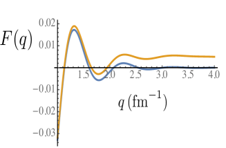
Figure 1: Nuclear Form Factor. Blue, solid, $F(q)$, Red, dashed, $F(q)+\Delta F(q)$.

IV Two-Nucleon Separation Distance

This section examines the physics of the two-nucleon separation distance. Bound-state wave functions are constructed using simple, two-parameter models of the ${}^{3}{\rm S}_{1}$ nucleon-nucleon interaction with parameters chosen to reproduce the measured scattering length and effective range Brown and Jackson (1976). As such, these are low-energy interactions. These simple potentials contain features such as a hard core or Yukawa interaction that have been parts of more realistic interactions. The range parameters of that reference are used here, with the strengths of the potential adjusted slightly so as to reproduce the value of the binding energy (2.2 MeV). The different potentials produce different bound-state wave functions and measurable differences are perceived through the behavior of the form factors (here the Fourier transforms of the square of the wave functions). The importance of the correction terms in the difference between using ${\cal O}_{s}$ and ${\cal O}$ is assessed. The scaling properties of the form factors are also presented in preparation for use in Sect. V.

IV.1 nucleon-nucleon hard core plus exponential potential

This potential is defined by having an infinite hard core at a separation $r_{0}$ and an attractive exponential potential $V(r)=-V_{0}\,e^{-(r-r_{0})/a}$ ($V_{0}=1.92\,\,\text{fm}^{-1}$) for larger separations. The model is exactly solvable. The values $r_{0}=0.4$ fm and $a=0.45$ Brown and Jackson (1976) are used. This potential (as others in this section) is a crude model for deuteron properties because there is no tensor force.

The $s$-state bound state wave function is determined by using the transformation $y=2a\gamma e^{-r/(2a)}$, $\gamma=\sqrt{MB}$, where $B$ is the binding energy and $M$ the nucleon mass, which converts the Schroedinger equation into Bessel’s equation. Then the bound-state wave function is

$$u(r)=N\,J_{2a\gamma}(2a\sqrt{MV_{0}}e^{-r/2a}),$$ (19)

subject to the condition that $u(r_{0})=0$. The factor $N$ is a normalization constant. One can check the large $r$ limit by using the small argument limit of the Bessel function ($J_{\nu}(x)\sim x^{\nu}$) so that $\lim_{r\to\infty}u(r)\propto e^{-\gamma r}$, as expected. The form factor of this model is the bound-state matrix element of the operator

$${\cal O}_{\bf Q}=e^{i{\bf Q}\cdot{\bf r}/2},$$ (20)

in which the probe is defined to act only on one nucleon of the two-body system. Then the form factor is given by

$$F(Q)={2\over Q}\int_{r_{0}}^{\infty}{dr\over r}{\sin{(Q/2\,r)}}u^{2}(r),$$ (21)

and can be re-expressed in terms of the momentum-space wave function $\psi(k)$ given by

$$\psi(k)={1\over\sqrt{2}\pi k}\int_{r_{0}}^{\infty}dr\sin{kr}\;u(r),$$ (22)

with

$$F(Q)=\int d^{3}k\,\psi(k_{+})\psi(k_{-}),$$ (23)

and ${\bf k}_{\pm}\equiv{\bf k}\pm{\bf Q}/4$.

If one uses the $V_{\rm low\,k}$ prescription of Eq. (2) one cuts off the momentum-space wave function at a relative momentum $\Lambda$, with $\Lambda=2.1$ fm^-1 a commonly used value. The aim here is to see how much of the form factor (as a function of $Q^{2}$) is given by relative momenta that are greater than $\Lambda$.

The cutoff form factor is then given by

$$F_{\Lambda}(Q)=\int d^{3}k\psi(k_{+})\psi(k_{-})\Theta(\Lambda-k_{+})\Theta(\Lambda-k_{-}).$$

(24)

Using this form factor corresponds to using Eq. (2) for the wave function. Invariance of the form factor would be obtained if the probe operator were modified according to Eq. (3) or Eq. (10). The purpose in computing $F_{\Lambda}(Q)$ is only to determine the values of $\Lambda$ for which operator modification becomes necessary.

Fig. 2 shows the form factor falling asymptotically as $1/Q^{6}$ and modulated by oscillations. Fig.  3 shows the values of $\Lambda$ necessary to achieve 5% accuracy in the form factor as a function of $Q$. These are greater than 2.1 $\,\text{fm}^{-1}$ for values of $Q>2.2$ fm^-1, so such values of $Q$ require operator modification. The use of Eq. (10) is not possible because of the hard core of the potential.

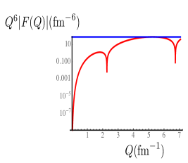
Figure 2: $F(Q)$ for hard core plus exponential potential

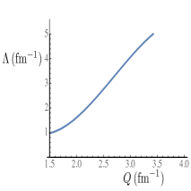
Figure 3: Value of $\Lambda$ for which $F_{\Lambda}(Q)/F_{\infty}(Q)=0.95$ as a function of $\Lambda$.

IV.2 Square well potential

The next example is the square well potential with a radius of 2.205 fm Brown and Jackson (1976) and depth 0.157 fm^-1. The form factor is shown in Fig. 4. Fig. 5 shows the values of $\Lambda$ necessary to achieve 5% accuracy in the form factor as a function of $Q$. Operator modification is found to be important here for values of $Q>1.5$ fm^-1. The use of Eq. (10) is not possible because the derivatives of the potential are delta functions.

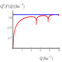
Figure 4: $F(Q)$ for square well potential

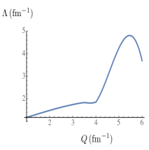
Figure 5: Value of $\Lambda$ for which $F_{\Lambda}(Q)/F_{\infty}(Q)=0.95$ as a function of $\Lambda$ for square well potential. The rapid rise is due to a node in the form factor.

IV.3 Exponential potential

The exponential potential is given by the expression $V(r)=-V_{0}e^{-r/a}$ with $a=0.76$ fm Brown and Jackson (1976) and $V_{0}=0.779$ fm^-1. The form factor is shown in Fig. 6. One sees that $F(Q)$ scales as $1/Q^{6}$.

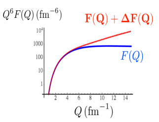
Figure 6: $Q^{6}F(Q)$ for exponential potential. Solid $F(Q)$. Dashed $F(Q)+\Delta F(Q)$, see Eq. (26).

This potential has well-defined derivatives so that one may use the probe operator evolution of Eq. (10) to study the change in the operator. For computing the form factor of a two-body bound state Eq. (10) becomes

$${\cal O}_{s}\approx(1-{i\over 2}sM{dV\over dr}(\hat{\bf r}\cdot{\bf Q}))e^{i{\bf Q}\cdot{\bf r}/2}.$$ (25)

The use of the second term of this equation causes a change to the computed form factor $\Delta F(Q)$ with

$$\Delta F(Q)={QsM\over 6}\int dru^{2}(r)j_{1}(Qr/2){dV\over dr}.$$ (26)

The function $F(Q)+\Delta F(Q)$ is shown as the dashed curve of Fig. 6. One sees that the term induced by the softening of the interaction causes a significant hardening of the interaction starting for values of $Q$ as low as about $2\,\text{fm}^{-1}$ and dominates for $Q>3$ fm${}^{-1}.$ If $\Delta F$ is large compared with $F$ it is necessary to include higher-order terms in $s$, so the details would change. Nevertheless, the Fig. 6 demonstrates the hardening of the probe interaction.

IV.4 Yukawa potential

Here $V(r)=V_{0}e^{-\mu r}/r$ with $\mu=0.411\,{\rm fm^{-1}}$ as in Brown and Jackson (1976) and $V_{0}=0.25$. The form factor, as shown Fig. 7, scales as $Q^{-4}$. The function $F(Q)+\Delta F(Q)$ (Eq. (26)) is shown as the rising curve of Fig. 7. The dramatic change in the probe operator is caused by the large derivative of the Yukawa potential at short distances. The Fig. 7 again demonstrates the hardening of the probe interaction.

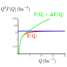
Figure 7: $Q^{4}F(Q)$ and $Q^{4}(F(Q)+\Delta F(Q))$ for Yukawa potential.

IV.5 Influence of tensor force and higher $Q^{2}$

The one-pion exchange potential (OPEP) causes a tensor force that dominates the long range properties of the deuteron. This has been known since the discovery of the quadrupole moment of the deuteron in 1939. Furthermore, the OPEP by itself, along with a single parameter that provides a short-distance cutoff, is known to provide an approximate but reasonable bound state wave function for the deuteron Friar et al. (1984); Cooke and Miller (2002).

The iteration of the tensor part of OPEP that occurs in solving the Schroedinger equation gives an S-state potential that acts approximately as an atractive delta function potential Kaiser et al. (2002); Hen et al. (2015, 2017). This approximate delta function is the leading order term for the potential in both EFT and pionless EFT. In momentum space the S-state wave function has a node around $k=2$ fm ^-1, and the D-state dominates for $k$ between about 2 and 4 fm^-1 for many potentials that are in use in many-body calculations today.

The softening of the OPEP by the SRG means that the electromagnetic interaction must acquire a tensor force component. Including this effect in the probe operator would add a complication.

IV.6 Summary

Softening of the NN interaction via a unitary transformation or projection operator procedure requires a corresponding transformation of interaction operators that increases their effects at high momentum transfer. The examples shown indicate that for some potentials the effects of transforming the operator are very important for momentum transfers greater than about 5 fm^-1, an important region for current experiments that attempt to discover new phenomena. Furthermore, the transformed operators cannot be obtained easily for some potentials.

The use of the impulse approximation that involves using bare, untransformed operators simplifies the interpretation of experiments and therefore seems best suited for discovery purposes.

V Two-nucleon separation in nuclei: observing high momentum and short-distance features.

The previous Section discusses how high momentum components may arise from interactions between nucleons. The present Section is concerned with the manifestation of such effects in nuclei, and also one way to observe the relation between short-distance and high momentum physics.

Bethe Bethe (1956) wrote that “Indeed, it is well established that the forces between two nucleons are of short range, and of very great strength” and “there are strong arguments to show that the two-body forces continue to exist inside a complex nucleus ”.

Brueckner, Eden, and Francis, Brueckner et al. (1955) used a variety of nuclear reactions to argue that the nuclear wave function contains nucleons with a significant probability to have high momentum. One particularly telling example is the significant cross sections observed in the $(p,d)$ reaction with 95 MeV protons. The neutron in the nucleus must have high momentum comparable to that of the proton, about 420 MeV/c, so that combination with the incident proton allows the deuteron to emerge from the nucleus. The only way a bound neutron could acquire such momentum is via interactions with another nearby nucleon.

Bethe continued “All these processes show that the ‘potential’ is fluctuating violently from point to point in the nucleus, which is compatible with the assumption that two-body forces continue to act inside the nucleus without much modificcation.” The idea of two strongly interacting nucleons, acting independently of the other nucleons (the independent pair approximation) is the basis of Bruckner theory  Brueckner (1955) which provided a fundamental explanation of how nuclear saturation and the shell model of nuclei arise from fundamental, hard, short-ranged interactions of nucleons. This means that the nucleon-nucleon separation distance is related, via the nucleon-nucleon interaction, to the size of the entire nucleus.

One modern implementation of the independent pair approximation is the generalized contact formalism (GCF) Cruz-Torres et al. (2019). The GCF is an effective model that provides a factorized approximation for the short-distance (small-$r$) and high-momentum (large-$k$) components of the nuclear many-body wave function. Its derivation relies on the strong relative interaction of closely separated nucleons and their weaker interaction with the residual $A-2$ nuclear system Weiss et al. (2015, 2018); Cohen et al. (2018). Using this approximation, the two-nucleon density in either coordinate or momentum space (i.e., the probability of finding two nucleons with separation $r$ or relative momentum $q$) has been expressed at small separation or high momentum as Weiss et al. (2018):

$$\rho_{A}^{NN,\alpha}(r) =C_{A}^{NN,\alpha}\times|\varphi_{NN}^{\alpha}(r)|^{2},$$

$$n_{A}^{NN,\alpha}(k) =C_{A}^{NN,\alpha}\times|\varphi_{NN}^{\alpha}(k)|^{2},$$ (27)

where $A$ denotes the nucleus, $NN$ denotes the nucleon pair being considered ($pn$, $pp$, $nn$), and $\alpha$ stands for the nucleon-pair quantum state (spin 0 or 1). $C_{A}^{NN,\alpha}$ are nucleus-dependent scaling coefficients, referred to as “nuclear contact terms”, and $\varphi_{NN}^{\alpha}$ are two-body wave functions that are given by the zero-energy solution of the two-body Schrödinger equation for the $NN$ pair in the state $\alpha$. The functions $\varphi_{NN}^{\alpha}$ do not depend on the nucleus, but do depend on the $NN$ interaction.

The authors Cruz-Torres et al. (2019) state that an important feature of the GCF is the equivalence between short distance and high momentum, which is built into Eq. (27) by using the same contact terms $C_{A}^{NN,\alpha}$ for both densities. This equivalence is established by extracting the contacts separately from the coordinate- and momentum-space nuclear wave functions. The present section is devoted to finding a direct correspondence between short distance and high momentum.

This analysis uses the zero-energy Lippmann-Schwinger (LS) equation and asymptotic expansions obtained by integration by parts Erdelyi (1956). The LS equation for scattering at 0 energy is given by

$$\varphi_{NN}^{\alpha}(k)={-M\over k^{2}}\int{d^{3}r\over(2\pi)^{3/2}}e^{-i{\bf k}\cdot{\bf r}}V(r)\varphi_{NN}^{\alpha}(r).$$ (28)

If the potential is an approximate delta function in coordinate space, then $\varphi_{NN}^{\alpha}(k)\sim{1\over k^{2}}.$

For other interactions it is useful to express the $S$-wave, momentum-space wave function as:

$$\psi(k)=-{M\over\sqrt{2}\pi k^{3}}\int_{0}^{\infty}dr\sin({kr)}\ V(r)\ u(r),$$ (29)

where $u(r)$ is the S-state radial wave function and in which the labels $NN,\alpha$ are suppressed. One derives expansions for asymptotic values of the momenta by replacing the $\sin(kr)$ appearing in the integral of Eq. (29) by ${-1\over k}{d\cos kr\over dr}$. Then one can get higher-order terms by writing $\cos(kr)={1\over k}{d\sin{kr}\over kr}$. The result, defining $K\equiv{M\over\sqrt{2}\pi}$, assuming that the potential is not a delta function, and that $Vu$ and its derivatives exist at $r=0$ is:

$$\psi(k)={K\over k^{4}}\int_{0}^{\infty}dr{d\cos kr\over dr}V(r)u(r)$$ (30)

$$={K\over k^{2}}[-V(0)u(0)-\int_{0}^{\infty}dr\cos kr(Vu)^{\prime}]$$

$$={K\over k^{4}}V(0)u(0)+{K\over k^{6}}(Vu)^{\prime\prime}(0)+{K\over k^{8}}(Vu)^{\prime\prime\prime\prime}(0)+\cdots$$ (31)

If the potential is non-local of the form $V(r,r^{\prime})$ the product $Vu$ in Eq. (29) is replaced by

$$V_{u}(r)\equiv r\int_{0}^{\infty}dr^{\prime}V(r,r^{\prime})u(r^{\prime})$$ (32)

and the derivatives thereof that appear in Eq. (31) are replaced by derivatives of $V_{u}$ at the origin.

One may classify the asymptotic behavior obtained from different classes of potentials.

• Class I: The potential is a delta function. Then $\psi(k)\sim{1\over k^{2}}$ as in leading-order pion-less effective field theory. Or as in Ref Hammer et al. (2020) showing that an approximate delta-function potential arises from treating the iterated effects of the one pion exchange potential.

• Class II: $u(0)=0$ but $V(0)u(0)\neq 0.$ An example is $V\sim 1/r$ and $u(r)\sim r$ for small values of $r$. In this case, $\psi(k)\sim{V(0)u(0)\over k^{4}}$

• Class III: $u(0)=0$, $V(0)u(0)=0.$ An example is the exponential potential for which $V(0)\neq 0$ is finite and $u(0)=0$. In this case, $\psi(k)\sim{V^{\prime}(0)u^{\prime}(0)\over k^{6}}$

• Class IV: The potential has a hard core potential, infinitely repulsive for a distance less than a core radius, $r=c$. Then using $u(c)=0$, $u^{\prime}(c)\neq 0$ and taking the Fourier transform of the wave function:

  $$\psi(k)={-K\over k^{2}}\int_{c}^{\infty}dr{d\cos kr\over dr}u(r)$$

  $$\sim{K\over k^{3}}\sin(kc)u^{\prime}(c).$$ (33)

• Class V: $Vu$ and all of its derivatives vanish at the origin. This is the square well of range $R$. Then using the LS equation yields

  $$\psi(k)\sim{KV(0)\over k^{4}}\cos(kR)u(R).$$ (34)

• Class VI: Non-local potentials. The quantity $\psi(k)\propto\lim_{r\to 0}(V_{u}(r))/k^{4}$ unless the limit vanishes. The Yamaguchi potential  Yamaguchi and Yamaguchi (1955) $V(r,r^{\prime})\propto{e^{-\mu r}\over r}{e^{-\mu r^{\prime}}\over r^{\prime}}$ provides an example of $\psi(k)\propto{1\over k^{4}}$. A power law fall-off would be obtained even if previous limit did vanish because some non-zero even-numbered derivatives of $V_{u}$ at the origin must occur.

In each of the first five cases the product of the potential and wave function at short separation distances determines the high-momentum behavior of the momentum-space wave function. For non-local potentials the high-momentum behavior is controlled by $V_{u}$ and/or its derivatives at the origin. Once, again short-distance behavior determines the high momentum content. Moreover, in each case there is a power law fall-off with increasing $k$. This slow fall with increasing $k$ means that significant high-momentum content can be expected for all of the interactions of Classes I through VI.

A power-law fall off can be uniquely avoided if the potential is a function of $r^{2}$. In that case, all of the terms in the series of Eq. (31) would vanish because of the vanishing of all odd-number derivatives of $V(r^{2})$ at the origin. No realistic nucleon-nucleon potential in current use is a function of $r^{2}$. This means that significant high momentum content can be expected.

V.1 Form factors at high momentum transfer

The previous analysis of zero-energy wave functions is also applicable to bound-state wave functions. For a binding energy $B$ the $-M\over{k^{2n}}$ factors of Eq. (31) is replaced by $-{M\over(k^{2}+MB)k^{2n-2}}\approx-{M\over k^{2n}}$ in asymptotic expansions.

An approximate relation between the momentum space wave function and the elastic form factor can be obtained using Eq. (23). Ref. Brodsky and Lepage (1989) argued that the dominant contributions to the integral occur when ${\bf k}=\pm{\bf Q}/4$. Then

$$F(Q)\propto\psi(Q/4).$$ (35)

This result depends on factorizing the momentum dependence of the potential, $\tilde{V}$ from that of the wave function, and is denoted the factorization approximation. The procedure is to use the LS equation to represent the wave functions appearing in Eq. (24). Then Eq. (35) emerges if

$$\int d^{3}k\tilde{V}(|{\bf Q}/4-{\bf k}|)\psi(k)\approx\tilde{V}(Q/4)\int d^{3}k\psi(k).$$ (36)

The integral over $d^{3}k$ is the wave function at the origin of coordinate space.

The result Eq. (35) is remarkable. It means that under certain conditions, in principle, it is possible to measure the wave function of a system, or at least its momentum dependence in a specific regime. This means that general statements about the unmeasurable nature of wave functions are not correct.

An (unrealistic) experiment in which one could attempt to test Eq. (35) is elastic electron scattering from a $b\overline{b}$ meson. Elastic scattering on the deuteron is complicated by the need to include the effects of meson exchange currents and corrections to the non-relativistic treatment Marcucci et al. (2016). Calculations of deuteron form factors for momentum transfers greater than about 7 fm^-1 are not shown in that review.

Note also that nucleon-nucleon scattering at laboratory energies less than 350 MeV does not yield significant constraints on $\tilde{V}(Q/4)$ for large values of $Q$ Miller and Strikman (2004). Large momentum transfer means that large kinetic energy is needed.

The following text explains how the different classes of potentials discussed here can be or cannot be manifest by measurements of form factors as expressed in Eq. (35).

Class I: $V$ is a delta function in coordinate space, and therefore a constant in momentum space. The wave function $\psi(k)$ is mainly determined by the propagator in which $k$ and $Q$ of Eq. (36) of the same importance. The factorization argument does not apply.

Class II: The Yukawa potential $V(r)=V_{0}e^{-\mu r}/r$. The product $Vu$ is well defined as $r\to 0$, because then $u(r)\propto r$. Thus Eq. (31) predicts $\psi(Q)\sim 1/Q^{4}$ and the form factor show in in Fig. 7 also shows a $1/Q^{4}$ behavior.

Class III: The exponential potential. In accord with Eq. (31) the wave function falls as $1/Q^{6}$, and so does the form factor shown in Fig. 6.

Class IV: Hard core plus exponential. Fig. 2 shows oscillations expected from Eq. (33) but factorization does not work because the discontinuity of $u^{\prime}(r)$ at $r=r_{0}$ induces large momentum components.

Class V: Square well potential. The factorization approximation is not accurate, although oscillations with period $(2\pi/R\approx 3\,{\rm fm}^{-1}$ are seen. This is because condition of Eq. (36) are not maintained due to oscillations that cause 0’s in $\tilde{V}$ for large values of the argument.

In summary, the short distance behavior of the potential times the coordinate-space radial wave function determines the high momentum dynamics in all cases. If the factorization approximation of Eq. (36) is valid and the probe operator is well-known the measurement of the form factor determines the high-momentum behavior of the wave function.

VI The $(e,e^{\prime}p)$ reaction: discovery at the nucleon-nucleon separation scale

The $(e,e^{\prime}p)$ reaction occurs if an electron knocks out a nucleon so that an initial nuclear state of $A$ nucleons is converted to a final nuclear state of $A-1$ nucleons.

In the plane wave impulse approximation (PWIA), an electron transfers a single virtual photon with momentum ${\bf q}$ and energy $\nu$ to a single proton, which then leaves the nucleus without interacting with another nucleon on the way out of the nucleus, see Fig. 10. There are various corrections- final state interactions, meson exchange currents etc. However, one can account for such effects by using appropriate kinematics and including the effects of final state interactions, see e.g. Schmidt et al. (2020).

For high-momentum transfer processes the outgoing nucleon has high energy, greater than the 350 MeV that is used to constrain nucleon-nucleon potentials. The softening effects of unitary transformations on nucleon-nucleon potentials requires that the potential be Hermitian. No realistic Hermitian potential applicable for scattering energies greater than about 1.5 GeV exists at the present time. This means applying a unitary transformation to soften the interaction is not practical. Instead, the final state interactions can be treated using the Glauber approximation in which the nucleon-nucleon scattering cross sections are used as input to form the optical potential Glauber and Matthiae (1970).

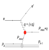
Figure 8: A nucleus emits a nucleon of four-momentum $P_{\rm miss}$ that absorbs a virtual photon of four-momentum $q$ to make a final-state nucleon of four-momentum $P_{\rm miss}+q$, with $(P_{\rm miss}+q)^{2}=M^{2}$, where $M$ is the nucleon mass.

If the background effects mentioned above are handled correctly, the scattering amplitude is proportional to the wave function of the struck bound nucleon Walecka (1995):

$${\cal M}\propto\psi(P_{\rm miss}).$$ (37)

Once again (as in Eq. (35)) the scattering amplitude is seen to directly accesses information about the momentum dependence of the wave function. This feature has enabled experimental studies to show that the high momentum part of the wave function is dominated by short-range correlations (SRCs) Fomin et al. (2017). These are pairs of nucleons with large relative and individual momenta and smaller center-of-mass (c.m.) momenta, where large is measured relative to the typical nuclear Fermi momentum $k_{F}\approx 250\,\rm MeV/c$ Hen et al. (2017); Ciofi degli Atti (2015). At momenta just above $k_{F}$ $(300\leq k\leq 600\,\rm MeV/c)$, SRCs are dominated by $pn$ pairs Tang et al. (2003); Piasetzky et al. (2006); Subedi et al. (2008); Korover et al. (2014); Hen et al. (2014); Duer et al. (2018, 2019). This $pn$ dominance is due to the tensor part of the nucleon-nucleon ($NN$) interaction Schiavilla et al. (2007); Alvioli et al. (2008).

The presence of nucleon-nucleon short ranged correlations in nuclei has many implications for the internal structure of nucleons bound in nuclei Hen et al. (2013, 2017); Schmookler et al. (2019), neutrinoless double beta decay matrix elements Kortelainen and Suhonen (2007a, b); Menendez et al. (2009); Simkovic et al. (2009); Benhar et al. (2014); Cruz-Torres et al. (2018); Wang et al. (2019), nuclear charge radii Miller et al. (2019), and the nuclear symmetry energy and neutron star properties Li et al. (2018).

If SRG transformations are applied to the strong-interaction Hamiltonian, the necessary use of hardened interactions (discussed in Sect. V) in analyzing experiments would complicate their interpretation.

VII Virtuality -a small-distance scale

Bound nucleons (of four momentum $p$) do not obey the standard Einstein relation $p_{\mu}p^{\mu}=M^{2}$, and are said to be off the mass shell. The average binding energy is much, much less than the nucleon mass, so the violation of the Einstein relation can be ignored when computing or understanding many average nuclear properties.

If one looks in more detail and examines nucleon-nucleon scattering, one sees that the intermediate nucleons must be off their mass shell. In the Blankenbecler-Sugar Blankenbecler and Sugar (1966) and Thompson reductions Thompson (1970) of the Bethe-Salpeter equation Salpeter and Bethe (1951) one nucleon emits a meson of 0 energy and non-zero momentum and the other nucleon absorbs the meson. Since the momenta of the nucleons have changed, but their energy hasn’t changed, the intermediate nucleons are off their mass shell. In other reductions of the Bethe-Salpeter equation Gross (1969), one nucleon is on the mass shell, and the other is not. This means that the nuclear wave function, treated relativistically, contains nucleons that are off their mass shell. Such nucleons must undergo interactions before they can be observed, and are denoted as virtual. The difference $p^{2}-M^{2}$ is related to the virtuality Miller (2019).

Experiments Egiyan et al. (2003, 2006); Fomin et al. (2012) using leptonic probes at large values of Bjorken $x$ interrogate the virtuality of the bound nucleons. To see this, consider the PWIA situation with $(P_{\rm miss}+q)^{2}=M^{2}$, let $q$ have the four-momentum $(\nu,{\bf 0}_{\perp},-\sqrt{\nu^{2}+Q^{2}}))\approx(\nu,{\bf 0}_{\perp},-(\nu+{Q^{2}\over 2\nu})$, in the Bjorken limit with $q^{2}=-Q^{2}$, $Q^{2}\to\infty,\,\nu\to\infty$, and $Q^{2}/\nu$ finite. Then with $q^{-}=q^{0}-q^{3}\approx 2\nu\gg q^{+}\approx-Mx$, $x={Q^{2}\over 2M\nu}$, one finds that

$${\cal V}\equiv{P_{\rm miss}^{2}-M^{2}\over M^{2}}\approx-{Q^{2}\over M^{2}}({P_{\rm miss}^{+}\over M}-1).$$ (38)

This quantity ${\cal V}$, defined here as the virtuality, is generally not zero. For example, experiments have been done with $Q^{2}=3$ GeV², ${P_{\rm miss}^{+}\over M}=1.5$ for which ${\cal V}\approx-1.5$. Plateaus, kinematically corresponding to to scattering by a pair of nucleons, have been observed Fomin et al. (2017) in this region. Treating highly virtual nucleons requires including relativistic effects. A recent study is Weiss et al. (2020).

The only way for a nucleon to be so far off the mass shell is for it to be interacting strongly with another nearby nucleon. To see that, consider a configuration of two bound nucleons, initially at rest in the nucleus. This is a good approximation for roughly 80% of the nuclear wave function. To acquire the large missing momentum of the previous paragraph, one nucleon must exchange a boson or bosons with four-momentum comparable to that of the incident virtual photon as shown in Fig. 10.

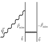
Figure 9: The strong interaction represented by the wiggly line exchanges a momentum $\vec{P}_{\rm miss}$ between two nucleons.

Such a bosonic system can only travel a short distance $\Delta r$ between the nucleons with

$$\Delta r\sim{1\over|\vec{P}_{\rm miss}|}.$$ (39)

Thus a highly virtual nucleon gets its virtuality from another nearby nucleon which must be closely separated. High virtuality is a short-distance phenomenon. As such, it serves as an intermediate step between using nucleonic and quark degrees of freedom

Ref. Arrington and Fomin (2019) attempted to find a difference between the effects of highly virtual nucleons and the effects of high local density. The simple arguments presented here show that there is a direct connection between high local density and high virtuality. It is therefore not possible to distinguish the two effects. This issue is discussed in more detail in Ref. Hen et al. (2019).

In evaluating Feynman diagrams the lowest-order effects of the non-vanishing of $\cal V$ can be cancelled by propagators and re-organized into low energy constants See Fig. 10. But understanding the fundamental origin of virtuality would allow a deeper understanding of nuclear physics.

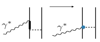
Figure 10: The effects of a virtual intermediate nucleon (indicated by the heavy line) may be replaced by using a two-nucleon contact interaction.

To better understand the connection between virtuality and quark degrees of freedom, consider a virtual nucleon as a superposition of physical states that are eigenfunction of the QCD Hamiltonian. Virtual states with nucleon quantum numbers can be expressed using the completeness of states of QCD:

$$|N({\cal V})\rangle=\sum_{n=1}^{n_{\rm max}}c_{n}|N_{n}\rangle,$$ (40)

in which the states $|N_{n}\rangle$ are resonances and also nucleon-multi-pion states. Each of these states has a detailed underlying structure in terms of quarks and gluons. In exclusive reactions with not very large momentum transfer few states are excited and one may use Eq. (40) to describe the physics. However, for high energy inclusive reactions of experimental relevance one needs many states. In this case a quark description is necessary.

VIII EMC effect- discovery at the small nuclear distance scale

The aim of this Section is to exemplify the connection between the small-distance scale related to virtuality and deep inelastic scattering from nuclei. The relation between virtuality and the EMC effect has been explored previously in Refs. Melnitchouk et al. (1994); Kulagin and Petti (2006); Ciofi degli Atti et al. (2007); Hen et al. (2017); Segarra et al. (2020).

Deep inelastic scattering (DIS) on a free nucleon target was initially expected to observe a set of resonances and therefore small cross sections for large values of three-momentum transfer  Bloom et al. (1969); Friedman and Kendall (1972). Instead, the cross sections were large an approximate Bjorken scaling was observed. The unambiguous interpretation is that the nucleon contains quarks.

I explain in more detail. For typical DIS kinematics $Q^{2}=100$ GeV${}^{2},\,x=0.5,\,\nu\approx$100 GeV, the expansion of Eq. (40) becomes unwieldy because the absorption of a virtual photon by free nucleon leads to a system of mass $M_{X}$ with $M_{X}^{2}=Q^{2}({1\over x}-1)$, so $M_{X}\approx 10$ GeV. This high excitation energy tells us that a huge number of baryon states are involved. Instead it is far more efficient to analyze the cross sections using quark degrees of freedom. Measurements determine the quark structure functions $q(x)$ that are scale and scheme dependent Tanabashi et al. (2018). However, they are well understood and interpreted as momentum distributions. Observe again that measurements of experimental cross sections determine features of wave functions.

Next turn to deep inelastic scattering on nuclei at similarly large values of $Q^{2}$. It was initially thought that at such kinematics only very small distances in the target would be involved Aubert et al. (1983). Such distances are much, much less than the internucleon spacing of $\approx$1.7 fm, and the expectation was that using a nuclear target would only increase the number of target nucleons. Instead, the medium modification of $q(x)$ was observed. At high values of $x$ the ratio of the bound to free structure function ratio is less than one by an amount of only between 10 and 15%, dependent on the nucleus. This effect is known as the EMC effect Aubert et al. (1983); Gomez et al. (1994).

That bound structure functions are different than free ones is natural in terms of the discussion above regarding virtuality and Eq. (40). Bound nucleons are virtual and the states $|N_{n}\rangle$ have different structure functions than the nucleon.

Because of the large number of states entering in Eq. (40) it is most efficient to use quark degrees of freedom to understand DIS large values of $Q^{2}$. Then the free nucleon is regarded as a superposition of various configurations or Fock states, each with a different quark-gluon structure.

I simplify the discussion using a model inspired by the QCD physics of color transparency Frankfurt and Strikman (1985); Brodsky and de Teramond (1988); Ralston and Pire (1988); Jennings and Miller (1993). The infinite number of quark-gluon configurations of the proton are treated as two configurations, a large-sized, blob-like configuration, BLC, consisting of complicated configurations of many quarks and gluons, and a small-sized, point-like configuration, PLC, consisting of 3 quarks. The BLC can be thought of as an object that is similar to a nucleon. The PLC is meant to represent a three-quark system of small size that is responsible for the high-$x$ behavior of the distribution function. The smaller the number of quarks, the more likely one can carry a large momentum fraction. The small-sized configuration (with its small number of $q\overline{q}$ pairs) is very different than a low lying nucleon excitation. This two-component model is meant to serve as a simple schematic tool to enable qualitative understanding.

When placed in a nucleus, the blob-like configuration feels the usual nuclear attraction and its energy decreases. The point-like-configuration feels far less nuclear-attraction by virtue of color screening  Frankfurt et al. (1994) in which the effects of gluons emitted by small-sized configurations are cancelled in low-momentum transfer processes. The nuclear attraction increases the energy difference between the BLCs and the PLCs, therefore reducing the PLC probability Frankfurt and Strikman (1985). Reducing the probability of PLCs in the nucleus reduces the quark momenta, in qualitative agreement with the EMC effect.

Working out the consequences of the BLC-PLC model enables the connection between the EMC effect and virtuality to be clarified. The Hamiltonian for a free nucleon in the two-component model can be expressed schematically by the matrix

$$H_{0}=\left[\begin{array}[]{cc}E_{B}&V\\ V&E_{P}\end{array}\right],$$ (43)

where $B$ represents BLC and $P$ the PLC. The PLC is spatially much smaller than the BLC, so that $E_{P}\gg E_{B}$. The hard-interaction potential, $V$, connects the two components, causing the eigenstates of $H_{0}$ to be $|N\rangle$ and $|X\rangle$ rather than $|B\rangle$ and $|P\rangle$. In lowest-order perturbation theory, the eigenstates are given by

$$|N\rangle = |B\rangle+\epsilon|P\rangle,$$ (44)

$$|X\rangle = -\epsilon|B\rangle+|P\rangle,$$ (45)

with $\epsilon=V/(E_{B}-E_{P})\ll 1.$ It is natural to assume $|V|\ll E_{P}-E_{B}$, so that the nucleon is mainly $|B\rangle$ and its excited state is mainly $|P\rangle$. The notation $|X\rangle$ is used to denote the state that is mainly a PLC, which does not at all resemble a low-lying baryon resonance.

The quark structure function is the matrix element of the operator $\cal O_{\rm DIS}$ that is the imaginary part of the virtual-photon- quark Compton scattering amplitude. This operator acts on a single quark, so that

$$q(x)={1\over 1+\epsilon^{2}}\left(\langle B|{\cal O}_{\rm DIS}|B\rangle+\epsilon^{2}\langle P|{\cal O}_{\rm DIS}|P\rangle\right),$$ (46)

in which it is assumed that the single-quark operator does not connect the two very different states $|B\rangle$ and $|P\rangle$. Furthermore, the condition that the PLC dominates the structure function at large values of $x$ is enforced by defining a function $f(x)>0$ that monotonically increases as $x$ increases. In particular, let

$$\langle P|{\cal O}_{\rm DIS}|P\rangle\equiv f(x)\langle B|{\cal O}_{\rm DIS}|B\rangle,$$ (47)

so that

$$q(x)={1\over 1+\epsilon^{2}}\langle B|{\cal O}_{\rm DIS}|B\rangle(1+\epsilon^{2}f(x)).$$ (48)

The model quark distributions of de Teramond et al. (2018), based on light-front holographic QCD, may provide a realization of the simple relation Eq. (47). These incorporate Regge behavior at small $x$ and inclusive counting rules as $x$ approaches unity and is consistent with DIS measurements. The model provides quark distributions $q_{\tau}(x)$ (normalized to unity) as function of $\tau$, the number of constituents in the system:

$$q_{\tau}(x)=\frac{\Gamma\left(\tau-\frac{1}{2}\right)}{\sqrt{\pi}\Gamma(\tau-1)}\big{(}1-w(x)\big{)}^{\tau-2}\,w(x)^{-{\frac{1}{2}}}\,w^{\prime}(x),$$ (49)

with $w(x)=x^{1-x}e^{-a(1-x)^{2}}.$ The elastic form factors of this model fall asymptotically as $1/Q^{2\tau}$, and the slope of form factors as $Q^{2}=0$ is proportional to $\tau$. These features mean that an increase in the value of $\tau$ corresponds to an increase in effective size. The function $q_{3}$ represents a three quark system and is naturally associated with the PLC.

In Eq. (49) the function $q_{\tau}$ is normalized to unity. The $u$ and $d$ quark distributions at a scale $\mu_{0}=1.06\pm 0.15$ GeV are given by

$$u(x)={3\over 2}q_{3}(x)+{1\over 2}q_{4}(x)$$ (50)

$$d(x)=q_{4}(x),$$ (51)

with the $u(x)$ and $d(x)$ normalized to the flavor content of the proton. An excellent reproduction of measured structure functions and elastic form factors is obtained using only two components and the flavor-independent parameter $a=0.531\pm 0.037$. This gives some justification to the simple two-state picture of the present model.

The ratio $q_{3}(x)/q_{4}(x)=1/(1-w(x))$ which increases monotonically with increasing $x$, as expected by the intuition inherent in Eq. (47) with $df/dx>1$. It is therefore reasonable to associate the PLC ($q_{3}$) with becoming more important as the value of $x$ increases. In this model BLC is associated with $q_{4}$, and the PLC component occurs only with up quarks. The relevant combination for a nucleus with $N$ neutrons and $Z$ protons is proportional to $Z{3\over 2}(q_{3}(x)+q_{4}(x))+{N\over 4}(3q_{3}(x)+9q_{4}(x))$.

Now suppose the nucleon is bound to a nucleus. The nucleon feels an attractive nuclear potential, here represented by $H_{1}$, with

$$H_{1}=\left[\begin{array}[]{cc}U&0\\ 0&0\end{array}\right],$$ (54)

to represent the idea that only the large-sized component of the nucleon feels the influence of the nuclear attraction. The treatment of the nuclear interaction, $U$, as a number is clearly a simplification because the interaction necessarily varies with the relevant kinematics. The present model is similar to the model of Frankfurt and Strikman (1985), with the important difference that the medium effects enter as an amplitude instead of as a probability. See also Ref. Frank et al. (1996).

The complete Hamiltonian $H=H_{0}+H_{1}$ is:

$$H=\left[\begin{array}[]{cc}E_{B}-|U|&V\\ V&E_{P}\end{array}\right],$$ (57)

in which the attractive nature of the nuclear binding potential is emphasized. Then interactions with the nucleus increase the energy difference between the bare BLC and PLC states and thereby decreases the PLC probability.

The medium-modified nucleon and its excited state, $|N\rangle_{M}$ and $|X\rangle_{M}$, are now (again using first-order perturbation theory)

$$|N\rangle_{M} = |B\rangle+\epsilon_{M}|P\rangle\$$ (58)

$$|X\rangle_{M} = -\epsilon_{M}|B\rangle+|P\rangle,$$ (59)

where

$$\epsilon_{M}={V\over{E_{B}-|U|-E_{P}}}=\epsilon{E_{B}-E_{P}\over E_{B}-|U|-E_{P}}$$ (60)

and ${\epsilon_{M}\over\epsilon}={E_{B}-E_{P}\over E_{B}-|U|-E_{P}}<1$.

The difference

$$\epsilon_{M}-\epsilon\approx{|U|\over E_{B}-E_{P}}$$ (61)

is relevant for understanding the EMC effect because

$$|N\rangle_{M}=|N\rangle+(\epsilon_{M}-\epsilon)\langle P|{\cal O}_{\rm DIS}|P\rangle,$$ (62)

and the medium modification of the nucleon is proportional to the interaction with the nucleus represented by $U$.

The medium-modified quark distribution function $q_{M}(x)=\langle N_{M}|{{\cal O}_{\rm DIS}}|N_{M}\rangle$, and is $q_{M}(x)=q(x)+\Delta q(x)$ with

$$\Delta q\approx 2(\epsilon_{M}-\epsilon)\langle N|{{\cal O}_{\rm DIS}}|P\rangle$$

$$\approx 2(\epsilon_{M}-\epsilon)\epsilon\langle P|{{\cal O}_{\rm DIS}}|P\rangle.$$ (63)

in which terms of first-order in $(\epsilon_{M}-\epsilon)$ kept to represent the small EMC effect. Next use Eq. (47) and Eq. (48) to find

$$\Delta q(x)={2(\epsilon_{M}-\epsilon)\epsilon}\,{q(x)f(x)\over 1+\epsilon^{2}f(x)}$$

$$\approx{2(\epsilon_{M}-\epsilon)\epsilon}\,q(x)f(x)$$ (64)

Note that the product $(\epsilon_{M}-\epsilon)\epsilon$ is less than zero, independent of the sign of the interaction $V$. This means that, at large values of $x$, the quark structure function in the nucleus is less than that of a free nucleon, and decreases with increasing $x$ because $f(x)$ is monotonically increasing with increasing $x$. These features are inherent in the data for values of $x<0.7$.

The next step is to relate $(\epsilon_{M}-\epsilon)\propto U$ (via Eq. (61)) to the virtuality. Suppose a photon interacts with a virtual nucleon of four-momentum ${\bf P}_{\rm miss}$ The three-momentum ${\bf P}_{\rm miss}$ opposes the $A-1$ recoil momentum ${\bf p}\equiv{\bf P}_{\rm miss}=-{\bf P}_{A-1}$. The mass of the on-shell recoiling nucleus is given by $M_{A-1}^{*}=M_{A}-M+E,$ where $E>0$ represents the excitation energy of the spectator $A-1$ nucleus, to find Ciofi degli Atti et al. (2007)

$$M^{2}{\cal V}=P_{\rm miss}^{2}-M^{2}$$ (65)

$$=(M_{A}-\sqrt{(M_{A-1}^{*})^{2}+{\bf p}^{2}}\,)^{2}-{\bf p}^{2}-M^{2}$$ (66)

which reduces in the non-relativistic limit to

$$M^{2}{\cal V} \approx -2M\left({{\bf p}^{2}\over 2M_{r}}+E\right),$$ (67)

where the reduced mass $M_{r}=M(A-1)/A$. The virtuality, ${\cal V}$, is less than 0, and its magnitude increases with both the $A-1$ excitation energy and the initial momentum of the struck nucleon.

Refs. Frankfurt and Strikman (1985); Ciofi degli Atti et al. (2007) obtained a relation between the potential $U$ and the virtuality ${\cal V}$ by using the extension of the Schroedinger equation to an operator form:

$${{\bf p}^{2}\over 2M_{r}}+U=-E,$$ (68)

so that ${{\bf p}^{2}\over 2M_{r}}+E=-U=|U|$ and via Eq. (61)

$${\cal V}={2U\over M}={2(\epsilon_{M}-\epsilon)(E_{P}-E_{B})\over M},$$ (69)

so that the modification of the nucleon due to the PLC suppression is proportional to its virtuality. Potentially large values of the virtuality greatly enhance the difference between $\epsilon_{m}$ and $\epsilon$.

Recall Eq. (63) and replace $(\epsilon_{M}-\epsilon)$ therein by its expression in terms of ${\cal V}$ (Eq. (69)) to find

$$q_{M}(x)=q(x)+{M\over E_{P}-E_{B}}{\cal V}\epsilon\,f(x)q(x),$$ (70)

The conditions that $(\epsilon_{M}-\epsilon)\epsilon<0,\,{\cal V}<0$ and Eq. (69) lead to the requirement that $\epsilon>0$, which means that $V<0$. The sign of $\epsilon$ is consistent with the light-front holographic model for which $\epsilon=1/\sqrt{2}$ for the proton and 0 for the neutron. The suppression of point-like components is manifest by the condition $df/dx>0$ and $\epsilon df/dx>0$. The ratio of structure functions is $R(x)=q_{M}(x)/q(x)$, and

$${dR\over dx} = {M\over E_{P}-E_{B}}{\cal V}\epsilon{df\over dx}<0,$$ (71)

as the measurements of the EMC effect have shown. The negative sign is caused by the negative value of the virtuality. This expression is only meaningful for $x<0.7$ where Fermi motion effects can be ignored.

Table 1: EMC effect vs. Virtuality.

Quantity	3 He	4He	12C	56Fe	208Pb
$|{dR\over dx}|$ Weinstein et al. (2011).	0.070 $\pm$0.029	0.197$\pm 0.026$	0.292$\pm$0.023	0.388 $\pm$0.032	0.409$\pm$ 0.039
$|{{\cal V}\over 2M}|$ (MeV) Ciofi degli Atti et al. (2007)	34.59	69.4	82.28	82.44	92.2

The quantities $M,E_{P}-E_{B}$ and $f(x)$ are independent of the nucleus, so that the $A$-dependence of the EMC effect is determined by the virtuality, ${\cal V}$. According to this model, the larger the virtuality the larger the EMC effect, as measured by the slope of $R(x)$. Table I compares the measurements of the slope with computations of the virtuality. The data for A=56 is from a mixture of A=56 and A=63. The theory for ²⁰⁸Pb is compared with the data for ¹⁹⁷Au. The increase of the magnitude of the slope tracks qualitatively well with the corresponding increase of the virtuality. A quantitative reproduction of the A-dependence requires a more detailed treatment of the separate N and Z dependence as in Ref. Schmookler et al. (2019).

Another consequence of this model is that the medium-modified nucleon contains a component that is an excited state of a free nucleon. The amount of modification, $\epsilon_{M}-\epsilon$, which gives a deviation of the EMC ratio from unity, is controlled by the potential $U$ and via Eq. (69) the virtuality. A more detailed evaluation of the EMC effect is reserved for another paper.

IX Summary & Discussion

This paper takes a trip through three length scales relevant to nuclear physics. These are the nuclear size, the inter-nucleon separation distance and the nucleon size. Simple examples are used to illustrate the basic underlying features that drive the observations made at the three different scales. The intent is to arrive at the realization that all three scales are must be understood to truly understand the physics of nuclei.

Sect. II briefly reviews the currently popular procedure of softening the interactions between nucleons, with a focus on the concomitant hardening of the operators that probe nuclei. A first-order equation, Eq. (10) is derived to demonstrate that the probe operators are hardened by the same unitary transformation that softens the interactions.

Sec. III discusses the largest nuclear scale, with the first point being that momentum transfers higher than that achieved by Rutherford were needed to discern the non-zero nature of the nuclear size. Equations (Eq. (17) and Eq. (18)) are derived to estimate the effect of the hardening of the probe operator, and is used to demonstrate its importance for momentum transfers, $q$, greater than about 2 fm^-1.

The physics of the nucleon-nucleon separation is explored in Sect. IV by using bound-state wave functions produced by four simple models of the nucleon interaction. The high-momentum transfer ($q$) scaling of the form factors is exhibited for each model. The values of relative momentum $p$ that make important contributions to the form factor are displayed. Increasing the value of $q$ is shown to increase the values of $p$ that enter. The resulting effect of the hardening of the probe operator is displayed for two of the model interactions, where again significant effects of hardening of the operator are seen for $q>2$ fm^-1. For other interactions the hardening cannot be computed easily. The role of the tensor force in producing high-momentum components, and in transforming the probe operator, is also discussed. Current experiments involve transfer of high momentum. The interpretation of such experiments is simplified if bare, un-transformed probe operators can be used.

The role of two-nucleon physics in nuclei, as manifest in the independent pair approximation, is explored in Sect. V. The modern approach is the generalized contact formalism. The high-momentum properties of 0-energy wave functions entering that formalism are examined. The result Eq. (31) demonstrates the explicit connection between short-distance and high-momentum physics. Furthermore, the inevitable power-law falloff indicates that significant high momentum content must occur. The conditions necessary for obtaining a direct connection, Eq. (35), between scaling behavior of measured form factors and the underlying wave functions are determined.

Sect. VI discusses the $(e,e^{\prime},p)$ reaction as a tool for discovery of short-distance physics at the nucleon-nucleon separation scale. Under certain conditions Eq. (37), which directly relates the scattering amplitude to the wave function, is valid. More generally, at high momentum transfer, final state nucleons have high energy and undergo different interactions than those in the initial state. Thus, in such situations, it is far simpler to use the impulse approximation with the fundamental potentials in the Hamiltonian than to use interactions softened by unitary transformations.

The transition from the nucleon-nucleon separation distance to the nucleon size and smaller sizes is begun in Sect. VII through a discussion of virtuality, Eq. (38). High momentum transfer reactions probe highly virtual nucleons. Nucleons achieve high virtuality only through strong interactions with closely separated nucleons, Eq. (39). The internal wave function of such nucleons may be expressed as a superposition of baryonic eigenstates, Eq. (40). If the momentum transfer is large enough many, many states must be included in the superposition, and it becomes more efficient to use quark degrees of freedom.

The role of virtuality in understanding the nuclear modification of quark structure functions (EMC effect) is discussed in Sect. VIII. The explicit connection, Eq. (71) is displayed by using a two-component, (point-like/blob-like) model of the nucleon’s quark degrees of freedom. The simple model is shown to be consistent with the two-state treatment of light-front holographic QCD that reproduces free nucleon structure functions and elastic form factors. In particular, the point-like component is more important relative to the blob-like component at larger values of $x$. This model, combined with the concept of virtuality provides a qualitative explanation of the EMC effect.

X Appendix-Derivation of Eq. (10)

The result, Eq. (10) is stated without treating the term of first order in $s$ caused by the $s$-dependence of the potential. This Appendix shows that the term vanishes for the case of a local, bare potential and a local operator ${\cal O}$.

Consider the matrix element

$${\cal M}_{s}\equiv\langle\Psi|[H_{0},[V_{s},{\cal O}]]|\Psi\rangle,$$ (72)

which enters in computing elastic form factors. The goal here is to show that the term of order $s$ vanishes. To first order in $s$

$$V_{s}\approx V+s{dV\over ds}(s=0)=V+s[[H_{0},V],V].$$ (73)

The double commutator $[[H_{0},V],V]={-2\over M}(\mbox{\boldmath$\nabla$}V)^{2}$ which is function of ${\bf r}$. This commutes with ${\cal O}$ and Eq. (10) is obtained.

References

- Bohr and Mottelson (1998) A Bohr and B. R Mottelson, Nuclear Structure: Volume I: Single-Particle Motjon (World Scientific Publishing Co., Singapore, 1998).
- Georgi (1993) H. Georgi, “Effective field theory,” Ann. Rev. Nucl. Part. Sci. 43, 209–252 (1993).
- Cohen (2019) Timothy Cohen, “As Scales Become Separated: Lectures on Effective Field Theory,” PoS TASI2018, 011 (2019), arXiv:1903.03622 [hep-ph] .
- Bloom et al. (1969) Elliott D. Bloom et al., “High-Energy Inelastic e p Scattering at 6-Degrees and 10-Degrees,” Phys. Rev. Lett. 23, 930–934 (1969).
- Friedman and Kendall (1972) Jerome I. Friedman and Henry W. Kendall, “Deep inelastic electron scattering,” Ann. Rev. Nucl. Part. Sci. 22, 203–254 (1972).
- Bogner et al. (2003a) S.K. Bogner, T.T.S. Kuo, A. Schwenk, D.R. Entem, and R. Machleidt, “Towards a model independent low momentum nucleon nucleon interaction,” Phys. Lett. B 576, 265–272 (2003a), arXiv:nucl-th/0108041 .
- Bogner et al. (2003b) S.K. Bogner, T.T.S. Kuo, and A. Schwenk, “Model independent low momentum nucleon interaction from phase shift equivalence,” Phys. Rept. 386, 1–27 (2003b), arXiv:nucl-th/0305035 .
- Bogner et al. (2001) S.K. Bogner, A. Schwenk, T.T.S. Kuo, and G.E. Brown, “Renormalization group equation for low momentum effective nuclear interactions,” (2001), arXiv:nucl-th/0111042 .
- Nogga et al. (2004) Andreas Nogga, Scott K. Bogner, and Achim Schwenk, “Low-momentum interaction in few-nucleon systems,” Phys. Rev. C 70, 061002 (2004), arXiv:nucl-th/0405016 .
- Bogner et al. (2005) S.K. Bogner, A. Schwenk, R.J. Furnstahl, and A. Nogga, “Is nuclear matter perturbative with low-momentum interactions?” Nucl. Phys. A 763, 59–79 (2005), arXiv:nucl-th/0504043 .
- Bogner et al. (2010) S.K. Bogner, R.J. Furnstahl, and A. Schwenk, “From low-momentum interactions to nuclear structure,” Prog. Part. Nucl. Phys. 65, 94–147 (2010), arXiv:0912.3688 [nucl-th] .
- Glazek and Wilson (1993) Stanislaw D. Glazek and Kenneth G. Wilson, “Renormalization of Hamiltonians,” Phys. Rev. D 48, 5863–5872 (1993).
- Szpigel and Perry (2000) Sergio Szpigel and Robert J. Perry, “The Similarity renormalization group,” , 59–81 (2000), arXiv:hep-ph/0009071 .
- Bogner et al. (2007a) S.K. Bogner, R.J. Furnstahl, and R.J. Perry, “Similarity Renormalization Group for Nucleon-Nucleon Interactions,” Phys. Rev. C 75, 061001 (2007a), arXiv:nucl-th/0611045 .
- Jurgenson et al. (2008) E.D. Jurgenson, S.K. Bogner, R.J. Furnstahl, and R.J. Perry, “Decoupling in the Similarity Renormalization Group for Nucleon-Nucleon Forces,” Phys. Rev. C 78, 014003 (2008), arXiv:0711.4252 [nucl-th] .
- Jurgenson et al. (2009) E.D. Jurgenson, P. Navratil, and R.J. Furnstahl, “Evolution of Nuclear Many-Body Forces with the Similarity Renormalization Group,” Phys. Rev. Lett. 103, 082501 (2009), arXiv:0905.1873 [nucl-th] .
- Epelbaum et al. (2009) E. Epelbaum, H.-W. Hammer, and Ulf-G. Meißner, “Modern theory of nuclear forces,” Rev. Mod. Phys. 81, 1773–1825 (2009).
- Ishii et al. (2007) N. Ishii, S. Aoki, and T. Hatsuda, “Nuclear force from lattice qcd,” Phys. Rev. Lett. 99, 022001 (2007).
- Aoki et al. (2010) Sinya Aoki, Tetsuo Hatsuda, and Noriyoshi Ishii, “Theoretical Foundation of the Nuclear Force in QCD and its applications to Central and Tensor Forces in Quenched Lattice QCD Simulations,” Prog. Theor. Phys. 123, 89–128 (2010), arXiv:0909.5585 [hep-lat] .
- Murano et al. (2011) Keiko Murano, Noriyoshi Ishii, Sinya Aoki, and Tetsuo Hatsuda, “Nucleon-Nucleon Potential and its Non-locality in Lattice QCD,” Prog. Theor. Phys. 125, 1225–1240 (2011), arXiv:1103.0619 [hep-lat] .
- Doi et al. (2016) Takumi Doi et al., “First results of baryon interactions from lattice QCD with physical masses (1) – General overview and two-nucleon forces –,” PoS LATTICE2015, 086 (2016), arXiv:1512.01610 [hep-lat] .
- Aoki et al. (2018) Sinya Aoki, Takumi Doi, Tetsuo Hatsuda, and Noriyoshi Ishii, “Comment on “relation between scattering amplitude and bethe-salpeter wave function in quantum field theory”,” Phys. Rev. D 98, 038501 (2018).
- (23) Sinya Aoki, Takumi Doi, and Takumi Iritani, “Sanity check for bound states in lattice QCD,” EPJ Web Conf. 175, 10.1051/epjconf/201817505006, arXiv:1707.08800 [hep-lat] .
- Benhar and Pandharipande (1993) O. Benhar and V.R. Pandharipande, “Scattering of GeV electrons by light nuclei,” Phys. Rev. C 47, 2218–2227 (1993).
- Frankfurt et al. (1993) L. L. Frankfurt, M. I. Strikman, D. B. Day, and M. Sargsyan, “Evidence for short-range correlations from high (e,e’) reactions,” Phys. Rev. C 48, 2451–2461 (1993).
- Bogner et al. (2007b) S.K. Bogner, R.J. Furnstahl, R.J. Perry, and A. Schwenk, “Are low-energy nuclear observables sensitive to high-energy phase shifts?” Phys. Lett. B 649, 488–493 (2007b), arXiv:nucl-th/0701013 .
- Furnstahl and Hammer (2002) R.J. Furnstahl and H.W. Hammer, “Are occupation numbers observable?” Phys. Lett. B 531, 203–208 (2002), arXiv:nucl-th/0108069 .
- Sakurai and Napolitano (2017) Jun John Sakurai and Jim Napolitano, Modern Quantum Mechanics, Quantum physics, quantum information and quantum computation (Cambridge University Press, Cambridge, 2017).
- Gottfried et al. (2003) K Gottfried, , and T-M Yan, Quantum Mechanics: FUndamentals (Springer-Verlag, New York, 2003).
- Damascelli et al. (2003) Andrea Damascelli, Zahid Hussain, and Zhi-Xun Shen, “Angle-resolved photoemission studies of the cuprate superconductors,” Rev. Mod. Phys. 75, 473–541 (2003).
- Schmidt et al. (2020) A. Schmidt et al. (CLAS), “Probing the core of the strong nuclear interaction,” Nature 578, 540–544 (2020), arXiv:2004.11221 [nucl-ex] .
- Hen et al. (2017) O. Hen, Gerald. A. Miller, E. Piasetzky, and L.B. Weinstein, “Nucleon-Nucleon Correlations, Short-lived Excitations, and the Quarks Within,” Rev. Mod. Phys. 89, 045002 (2017), arXiv:1611.09748 [nucl-ex] .
- Avignone et al. (2008) Frank T. Avignone, Steven R. Elliott, and Jonathan Engel, “Double beta decay, majorana neutrinos, and neutrino mass,” Rev. Mod. Phys. 80, 481–516 (2008).
- Kozaczuk et al. (2017) Jonathan Kozaczuk, David E. Morrissey, and S.R. Stroberg, “Light axial vector bosons, nuclear transitions, and the 8Be anomaly,” Phys. Rev. D 95, 115024 (2017), arXiv:1612.01525 [hep-ph] .
- Ordonez and van Kolck (1992) C. Ordonez and U. van Kolck, “Chiral lagrangians and nuclear forces,” Phys. Lett. B 291, 459–464 (1992).
- Ordonez et al. (1994) C. Ordonez, L. Ray, and U. van Kolck, “Nucleon-nucleon potential from an effective chiral Lagrangian,” Phys. Rev. Lett. 72, 1982–1985 (1994).
- Ordonez et al. (1996) C. Ordonez, L. Ray, and U. van Kolck, “The Two nucleon potential from chiral Lagrangians,” Phys. Rev. C 53, 2086–2105 (1996), arXiv:hep-ph/9511380 .
- Bedaque and van Kolck (2002) Paulo F. Bedaque and Ubirajara van Kolck, “Effective field theory for few nucleon systems,” Ann. Rev. Nucl. Part. Sci. 52, 339–396 (2002), arXiv:nucl-th/0203055 .
- Hammer et al. (2020) H.-W. Hammer, Sebastian König, and U. van Kolck, “Nuclear effective field theory: Status and perspectives,” Rev. Mod. Phys. 92, 025004 (2020).
- Bogner et al. (2007c) S.K. Bogner, R.J. Furnstahl, S. Ramanan, and A. Schwenk, “Low-momentum interactions with smooth cutoffs,” Nucl. Phys. A 784, 79–103 (2007c), arXiv:nucl-th/0609003 .
- Anderson et al. (2010) E.R. Anderson, S.K. Bogner, R.J. Furnstahl, and R.J. Perry, “Operator Evolution via the Similarity Renormalization Group I: The Deuteron,” Phys. Rev. C 82, 054001 (2010), arXiv:1008.1569 [nucl-th] .
- Bogner et al. (2008) S.K. Bogner, R.J. Furnstahl, and A. Schwenk, “Comment on ‘Problems in the derivations of the renormalization group equation for the low momentum nucleon interactions’,” (2008), arXiv:0806.1365 [nucl-th] .
- Glazek and Maslowski (2002) Stanislaw D. Glazek and Tomasz Maslowski, “Renormalized Poincare algebra for effective particles in quantum field theory,” Phys. Rev. D 65, 065011 (2002), arXiv:hep-th/0110185 .
- Tropiano et al. (2020) A.J. Tropiano, S.K. Bogner, and R.J. Furnstahl, “Operator evolution from the similarity renormalization group and the Magnus expansion,” (2020), arXiv:2006.11186 [nucl-th] .
- Hofstadter (1956) Robert Hofstadter, “Electron scattering and nuclear structure,” Rev. Mod. Phys. 28, 214–254 (1956).
- Hofstadter (1957) R. Hofstadter, “Nuclear and nucleon scattering of high-energy electrons,” Ann. Rev. Nucl. Part. Sci. 7, 231–316 (1957).
- Miller (2009) Gerald A. Miller, “Electromagnetic Form Factors and Charge Densities From Hadrons to Nuclei,” Phys. Rev. C 80, 045210 (2009), arXiv:0908.1535 [nucl-th] .
- Bertulani (2007) Carlos Bertulani, “Nuclear physics in a nutshell,” Nuclear Physics in a Nutshell, by Carlos A. Bertulani. ISBN 978-0-691-12505-3. Published by Princeton University Press, Princeton, NJ USA, 2007. (2007).
- Gmitro et al. (1987) M. Gmitro, S. S. Kamalov, and R. Mach, “Momentum-space second-order optical potential for pion-nucleus elastic scattering,” Phys. Rev. C 36, 1105–1117 (1987).
- Hahn et al. (1956) Beat Hahn, D. G. Ravenhall, and Robert Hofstadter, “High-energy electron scattering and the charge distributions of selected nuclei,” Phys. Rev. 101, 1131–1142 (1956).
- Krane (1987) K.S. Krane, Introductory Nuclear Physics (Wiley, NY, 1987).
- Brown and Jackson (1976) G.E. Brown and A.D. Jackson, The Nucleon-Nucleon Interaction (North Holland Publishing Company, 1976).
- Friar et al. (1984) James Lewis Friar, B.F. Gibson, and G.L. Payne, “One Pion Exchange Potential Deuteron ,” Phys. Rev. C 30, 1084–1086 (1984).
- Cooke and Miller (2002) Jason R. Cooke and Gerald A. Miller, “Pion - only, chiral light front model of the deuteron,” Phys. Rev. C 65, 067001 (2002), arXiv:nucl-th/0112076 .
- Kaiser et al. (2002) Norbert Kaiser, S. Fritsch, and W. Weise, “Chiral dynamics and nuclear matter,” Nucl. Phys. A 697, 255–276 (2002), arXiv:nucl-th/0105057 .
- Hen et al. (2015) O. Hen, L.B. Weinstein, E. Piasetzky, G.A. Miller, M.M. Sargsian, and Y. Sagi, “Correlated fermions in nuclei and ultracold atomic gases,” Phys. Rev. C 92, 045205 (2015), arXiv:1407.8175 [nucl-ex] .
- Bethe (1956) H. A. Bethe, “Nuclear many-body problem,” Phys. Rev. 103, 1353–1390 (1956).
- Brueckner et al. (1955) K. A. Brueckner, R. J. Eden, and N. C. Francis, “High-energy reactions and the evidence for correlations in the nuclear ground-state wave function,” Phys. Rev. 98, 1445–1455 (1955).
- Brueckner (1955) K. A. Brueckner, “Two-body forces and nuclear saturation. iii. details of the structure of the nucleus,” Phys. Rev. 97, 1353–1366 (1955).
- Cruz-Torres et al. (2019) R. Cruz-Torres, D. Lonardoni, R. Weiss, N. Barnea, D.W. Higinbotham, E. Piasetzky, A. Schmidt, L.B. Weinstein, R.B. Wiringa, and O. Hen, “Scale and Scheme Independence and Position-Momentum Equivalence of Nuclear Short-Range Correlations,” (2019), arXiv:1907.03658 [nucl-th] .
- Weiss et al. (2015) Ronen Weiss, Betzalel Bazak, and Nir Barnea, “Generalized nuclear contacts and momentum distributions,” Phys. Rev. C 92, 054311 (2015), arXiv:1503.07047 [nucl-th] .
- Weiss et al. (2018) R. Weiss, R. Cruz-Torres, N. Barnea, E. Piasetzky, and O. Hen, “The nuclear contacts and short range correlations in nuclei,” Phys. Lett. B 780, 211–215 (2018), arXiv:1612.00923 [nucl-th] .
- Cohen et al. (2018) E.O. Cohen et al. (CLAS), “Center of Mass Motion of Short-Range Correlated Nucleon Pairs studied via the Reaction,” Phys. Rev. Lett. 121, 092501 (2018), arXiv:1805.01981 [nucl-ex] .
- Erdelyi (1956) A. Erdelyi, Asymptotic Expansions (Dover Publications, Mineola, NY, 1956).
- Yamaguchi and Yamaguchi (1955) Y. Yamaguchi and Y. Yamaguchi, “Photodisintegration of the deuteron,” Phys. Rev. 98, 69–70 (1955).
- Brodsky and Lepage (1989) Stanley J. Brodsky and G.Peter Lepage, “Exclusive Processes in Quantum Chromodynamics,” Adv. Ser. Direct. High Energy Phys. 5, 93–240 (1989).
- Marcucci et al. (2016) L.E. Marcucci, F. Gross, M.T. Pena, M. Piarulli, R. Schiavilla, I. Sick, A. Stadler, J.W. Van Orden, and M. Viviani, “Electromagnetic Structure of Few-Nucleon Ground States,” J. Phys. G 43, 023002 (2016), arXiv:1504.05063 [nucl-th] .
- Miller and Strikman (2004) Gerald A. Miller and Mark Strikman, “Relation between the deuteron form factor at high momentum transfer and the high energy neutron-proton scattering amplitude,” Phys. Rev. C 69, 044004 (2004).
- Glauber and Matthiae (1970) R.J. Glauber and G. Matthiae, “High-energy scattering of protons by nuclei,” Nucl. Phys. B 21, 135–157 (1970).
- Walecka (1995) J.D. Walecka, Theoretical nuclear and subnuclear physics (Oxford University Press, Oxford, 1995).
- Fomin et al. (2017) Nadia Fomin, Douglas Higinbotham, Misak Sargsian, and Patricia Solvignon, “New Results on Short-Range Correlations in Nuclei,” Ann. Rev. Nucl. Part. Sci. 67, 129–159 (2017), arXiv:1708.08581 [nucl-th] .
- Ciofi degli Atti (2015) Claudio Ciofi degli Atti, “In-medium short-range dynamics of nucleons: Recent theoretical and experimental advances,” Phys. Rept. 590, 1–85 (2015).
- Tang et al. (2003) A. Tang et al., “n-p short range correlations from (p,2p + n) measurements,” Phys. Rev. Lett. 90, 042301 (2003), arXiv:nucl-ex/0206003 .
- Piasetzky et al. (2006) E. Piasetzky, M. Sargsian, L. Frankfurt, M. Strikman, and J.W. Watson, “Evidence for the strong dominance of proton-neutron correlations in nuclei,” Phys. Rev. Lett. 97, 162504 (2006), arXiv:nucl-th/0604012 .
- Subedi et al. (2008) R. Subedi et al., “Probing Cold Dense Nuclear Matter,” Science 320, 1476–1478 (2008), arXiv:0908.1514 [nucl-ex] .
- Korover et al. (2014) I. Korover et al. (Lab Hall A), “Probing the Repulsive Core of the Nucleon-Nucleon Interaction via the Triple-Coincidence Reaction,” Phys. Rev. Lett. 113, 022501 (2014), arXiv:1401.6138 [nucl-ex] .
- Hen et al. (2014) O. Hen et al., “Momentum sharing in imbalanced Fermi systems,” Science 346, 614–617 (2014), arXiv:1412.0138 [nucl-ex] .
- Duer et al. (2018) M. Duer et al. (CLAS), “Probing high-momentum protons and neutrons in neutron-rich nuclei,” Nature 560, 617–621 (2018).
- Duer et al. (2019) M. Duer et al. (CLAS), “Direct Observation of Proton-Neutron Short-Range Correlation Dominance in Heavy Nuclei,” Phys. Rev. Lett. 122, 172502 (2019), arXiv:1810.05343 [nucl-ex] .
- Schiavilla et al. (2007) R. Schiavilla, Robert B. Wiringa, Steven C. Pieper, and J. Carlson, “Tensor Forces and the Ground-State Structure of Nuclei,” Phys. Rev. Lett. 98, 132501 (2007), arXiv:nucl-th/0611037 .
- Alvioli et al. (2008) M. Alvioli, C. Ciofi degli Atti, and H. Morita, “Proton-neutron and proton-proton correlations in medium-weight nuclei and the role of the tensor force,” Phys. Rev. Lett. 100, 162503 (2008).
- Hen et al. (2013) Or Hen, D.W. Higinbotham, Gerald A. Miller, Eli Piasetzky, and Lawrence B. Weinstein, “The EMC Effect and High Momentum Nucleons in Nuclei,” Int. J. Mod. Phys. E 22, 1330017 (2013), arXiv:1304.2813 [nucl-th] .
- Schmookler et al. (2019) B. Schmookler et al. (CLAS), “Modified structure of protons and neutrons in correlated pairs,” Nature 566, 354–358 (2019), arXiv:2004.12065 [nucl-ex] .
- Kortelainen and Suhonen (2007a) Markus Kortelainen and Jouni Suhonen, “Improved short-range correlations and 0 neutrino beta beta nuclear matrix elements of Ge-76 and Se-82,” Phys. Rev. C 75, 051303 (2007a), arXiv:0705.0469 [nucl-th] .
- Kortelainen and Suhonen (2007b) Markus Kortelainen and Jouni Suhonen, “Nuclear matrix elements of neutrinoless double beta decay with improved short-range correlations,” Phys. Rev. C 76, 024315 (2007b), arXiv:0708.0115 [nucl-th] .
- Menendez et al. (2009) J. Menendez, A. Poves, E. Caurier, and F. Nowacki, “Disassembling the Nuclear Matrix Elements of the Neutrinoless beta beta Decay,” Nucl. Phys. A 818, 139–151 (2009), arXiv:0801.3760 [nucl-th] .
- Simkovic et al. (2009) Fedor Simkovic, Amand Faessler, Herbert Muther, Vadim Rodin, and Markus Stauf, “The 0 nu bb-decay nuclear matrix elements with self-consistent short-range correlations,” Phys. Rev. C 79, 055501 (2009), arXiv:0902.0331 [nucl-th] .
- Benhar et al. (2014) Omar Benhar, Riccardo Biondi, and Enrico Speranza, “Short-range correlation effects on the nuclear matrix element of neutrinoless double- decay,” Phys. Rev. C 90, 065504 (2014), arXiv:1401.2030 [nucl-th] .
- Cruz-Torres et al. (2018) Reynier Cruz-Torres, Axel Schmidt, Gerald A. Miller, Lawrence B. Weinstein, Nir Barnea, Ronen Weiss, Eliezer Piasetzky, and O. Hen, “Short range correlations and the isospin dependence of nuclear correlation functions,” Phys. Lett. B 785, 304–308 (2018), arXiv:1710.07966 [nucl-th] .
- Wang et al. (2019) X.B. Wang, A.C. Hayes, J. Carlson, G.X. Dong, E. Mereghetti, S. Pastore, and R.B. Wiringa, “Comparison between Variational Monte Carlo and Shell Model Calculations of Neutrinoless Double Beta Decay Matrix Elements in Light Nuclei,” Phys. Lett. B 798, 134974 (2019), arXiv:1906.06662 [nucl-th] .
- Miller et al. (2019) Gerald.A. Miller, A. Beck, S. May-Tal Beck, L.B. Weinstein, E. Piasetzky, and O. Hen, “Can Long-Range Nuclear Properties Be Influenced By Short Range Interactions? A chiral dynamics estimate,” Phys. Lett. B 793, 360–364 (2019), arXiv:1805.12099 [nucl-th] .
- Li et al. (2018) Bao-An Li, Bao-Jun Cai, Lie-Wen Chen, and Jun Xu, “Nucleon Effective Masses in Neutron-Rich Matter,” Prog. Part. Nucl. Phys. 99, 29–119 (2018), arXiv:1801.01213 [nucl-th] .
- Blankenbecler and Sugar (1966) R. Blankenbecler and R. Sugar, “Linear integral equations for relativistic multichannel scattering,” Phys. Rev. 142, 1051–1059 (1966).
- Thompson (1970) R.H. Thompson, “Three-dimensional bethe-salpeter equation applied to the nucleon-nucleon interaction,” Phys. Rev. D 1, 110–117 (1970).
- Salpeter and Bethe (1951) E.E. Salpeter and H.A. Bethe, “A Relativistic equation for bound state problems,” Phys. Rev. 84, 1232–1242 (1951).
- Gross (1969) Franz Gross, “Three-dimensional covariant integral equations for low-energy systems,” Phys. Rev. 186, 1448–1462 (1969).
- Miller (2019) Gerald A. Miller, “Confinement in Nuclei and the Expanding Proton,” Phys. Rev. Lett. 123, 232003 (2019), arXiv:1907.00110 [nucl-th] .
- Egiyan et al. (2003) K.S. Egiyan et al. (CLAS), “Observation of nuclear scaling in the A(e, e-prime) reaction at x(B) greater than 1,” Phys. Rev. C 68, 014313 (2003), arXiv:nucl-ex/0301008 .
- Egiyan et al. (2006) K.S. Egiyan et al. (CLAS), “Measurement of 2- and 3-nucleon short range correlation probabilities in nuclei,” Phys. Rev. Lett. 96, 082501 (2006), arXiv:nucl-ex/0508026 .
- Fomin et al. (2012) N. Fomin et al., “New measurements of high-momentum nucleons and short-range structures in nuclei,” Phys. Rev. Lett. 108, 092502 (2012), arXiv:1107.3583 [nucl-ex] .
- Weiss et al. (2020) R. Weiss, A.W. Denniston, J.R. Pybus, O. Hen, E. Piasetzky, A. Schmidt, L.B. Weinstein, and N. Barnea, “Study of inclusive electron scattering scaling using the generalized contact formalism,” (2020), arXiv:2005.01621 [nucl-th] .
- Arrington and Fomin (2019) J. Arrington and N. Fomin, “Searching for flavor dependence in nuclear quark behavior,” Phys. Rev. Lett. 123, 042501 (2019).
- Hen et al. (2019) O. Hen, F. Hauenstein, D.W. Higinbotham, G.A. Miller, E. Piasetzky, A. Schmidt, E.P. Segarra, M. Strikman, and L.B. Weinstein, “Comment on ”Searching for flavor dependence in nuclear quark behavior”,” (2019), arXiv:1905.02172 [nucl-ex] .
- Melnitchouk et al. (1994) W. Melnitchouk, Andreas W. Schreiber, and Anthony William Thomas, “Deep inelastic scattering from off-shell nucleons,” Phys. Rev. D 49, 1183–1198 (1994), arXiv:nucl-th/9311008 .
- Kulagin and Petti (2006) Sergey A. Kulagin and R. Petti, “Global study of nuclear structure functions,” Nucl. Phys. A 765, 126–187 (2006), arXiv:hep-ph/0412425 .
- Ciofi degli Atti et al. (2007) C. Ciofi degli Atti, L.L. Frankfurt, L.P. Kaptari, and M.I. Strikman, “On the dependence of the wave function of a bound nucleon on its momentum and the EMC effect,” Phys. Rev. C 76, 055206 (2007), arXiv:0706.2937 [nucl-th] .
- Segarra et al. (2020) E.P. Segarra, J.R. Pybus, F. Hauenstein, D.W. Higinbotham, G.A. Miller, E. Piasetzky, A. Schmidt, M. Strikman, L.B. Weinstein, and O. Hen, “Short-Range Correlations and the Nuclear EMC Effect in Deuterium and Helium-3,” (2020), arXiv:2006.10249 [hep-ph] .
- Tanabashi et al. (2018) M. Tanabashi et al. (Particle Data Group), “Review of Particle Physics,” Phys. Rev. D 98, 030001 (2018).
- Aubert et al. (1983) J.J. Aubert et al. (European Muon), “The ratio of the nucleon structure functions for iron and deuterium,” Phys. Lett. B 123, 275–278 (1983).
- Gomez et al. (1994) J. Gomez et al., “Measurement of the A-dependence of deep inelastic electron scattering,” Phys. Rev. D 49, 4348–4372 (1994).
- Frankfurt and Strikman (1985) L.L. Frankfurt and M.I. Strikman, “Point-Like Configurations ,” Nucl. Phys. B 250, 143–176 (1985).
- Brodsky and de Teramond (1988) Stanley J. Brodsky and G.F. de Teramond, “Spin Correlations, QCD Color Transparency and Heavy Quark Thresholds in Proton Proton Scattering,” Phys. Rev. Lett. 60, 1924 (1988).
- Ralston and Pire (1988) John P. Ralston and Bernard Pire, “Fluctuating Proton Size and Oscillating Nuclear Transparency,” Phys. Rev. Lett. 61, 1823 (1988).
- Jennings and Miller (1993) B.K. Jennings and G.A. Miller, “Color transparency in (p, p p) reactions,” Phys. Lett. B 318, 7–13 (1993), arXiv:hep-ph/9305317 .
- Frankfurt et al. (1994) L.L. Frankfurt, G.A. Miller, and M. Strikman, “The Geometrical color optics of coherent high-energy processes,” Ann. Rev. Nucl. Part. Sci. 44, 501–560 (1994), arXiv:hep-ph/9407274 .
- de Teramond et al. (2018) Guy F. de Teramond, Tianbo Liu, Raza Sabbir Sufian, Hans Gunter Dosch, Stanley J. Brodsky, and Alexandre Deur (HLFHS), “Universality of Generalized Parton Distributions in Light-Front Holographic QCD,” Phys. Rev. Lett. 120, 182001 (2018), arXiv:1801.09154 [hep-ph] .
- Frank et al. (1996) M.R. Frank, B.K. Jennings, and G.A. Miller, “The Role of color neutrality in nuclear physics: Modifications of nucleonic wave functions,” Phys. Rev. C 54, 920–935 (1996), arXiv:nucl-th/9509030 .
- Weinstein et al. (2011) L.B. Weinstein, E. Piasetzky, D.W. Higinbotham, J. Gomez, O. Hen, and R. Shneor, “Short Range Correlations and the EMC Effect,” Phys. Rev. Lett. 106, 052301 (2011), arXiv:1009.5666 [hep-ph] .