Generalized hydrodynamics study of the one-dimensional Hubbard model:
Stationary clogging and proportionality of spin, charge, and energy currents

Abstract

In our previous work [Nozawa and Tsunetsugu, Phys. Rev. B 101, 035121 (2020)], we studied the quench dynamics in the one-dimensional Hubbard model based on the generalized hydrodynamics theory for a partitioning protocol and showed the presence of a clogging phenomenon. Clogging is a phenomenon where vanishing charge current coexists with nonzero energy current, and we found it for the initial conditions that the left half of the system is prepared to be half filling at high temperatures with the right half being empty. Clogging occurs at all the sites in the left half and lasts for a time proportional to its distance from the connection point. In this paper, we use various different initial conditions and discuss two issues. The first issue is the possibility of clogging in a stationary state. When the electron density in the right half is initially set nonzero, we found that the left half-filled part expands for various sets of parameters in the initial condition. This means that the clogging phenomenon occurs at all the sites in the long-time stationary state, and we also discuss its origin. In addition, stationary clogging is accompanied by a back current, namely, particle density current flows towards the high-density region. We also found that spin clogging occurs for some initial conditions, i.e., the vanishing spin current coexists with nonzero energy current. The second issue is the proportionality of spin and charge currents. We found two spatio-temporal regions where the current ratio is fixed to a nonzero constant. We numerically studied how the current ratio depends on various initial conditions. We also studied the ratio of charge and energy currents.

I Introduction

Understanding nonequilibrium phenomena in strongly correlated systems is an important and challenging issue, and one-dimensional (1D) integrable models have attracted attention because their infinite number of conserved quantities play an important role Calabrese_2016 . Recently, the generalized hydrodynamics (GHD) theory was proposed by the authors of Refs. PhysRevX.6.041065, ; PhysRevLett.117.207201, for studying nonequilibrium dynamics of integrable models, and its experimental confirmation was demonstrated for a 1D Bose gas system PhysRevLett.122.090601 . An infinite number of conserved quantities is also important in GHD, as time-evolution equations are formulated based on their continuity equations. The GHD can describe the time evolution of spatially inhomogeneous systems, and partitioning is a frequently used protocol rubin1971abnormal ; spohn1977stationary ; bernard2012energy ; Bernard2015 ; bhaseen2015energy ; PhysRevX.6.041065 ; PhysRevLett.117.207201 , because the equations for the time evolution are simple in that case. Two semi-infinite parts in different thermal equilibria are connected at the origin $x=0$ and time $t=0$, and the time evolution of the connected system is analyzed. By using this protocol, many aspects of nonequilibrium phenomena in integrable models have been studied, e.g., the time dependence of currents PhysRevX.6.041065 ; PhysRevLett.117.207201 ; fagotti2016charges ; PhysRevB.96.020403 ; doyon2017dynamics ; PhysRevB.97.045407 ; PhysRevLett.120.045301 ; PhysRevB.97.081111 ; Bertini_2018 ; PhysRevLett.120.176801 ; 10.21468/SciPostPhys.4.6.045 ; PhysRevB.98.075421 ; PhysRevB.99.014305 ; PhysRevB.99.174203 ; doi:10.1063/1.5096892 ; Bulchandani_2019 , Drude weights PhysRevLett.119.020602 ; PhysRevB.96.081118 ; SciPostPhys.3.6.039 , entanglements PhysRevB.97.245135 ; Bertini_ent ; PhysRevB.99.045150 ; 10.21468/SciPostPhys.7.1.005 , correlation functions of densities and currents PhysRevB.96.115124 ; 10.21468/SciPostPhys.5.5.054 , diffusive dynamics and diffusion constants PhysRevLett.121.230602 ; PhysRevLett.121.160603 ; PhysRevB.98.220303 ; 10.21468/SciPostPhys.6.4.049 ; PhysRevLett.122.127202 ; Gopalakrishnan16250 ; PhysRevB.102.115121 .

The 1D Hubbard model is a canonical lattice model of strongly correlated electrons and is exactly solvable through the nested Bethe ansatz PhysRevLett.19.1312 ; GAUDIN196755 ; PhysRevLett.21.192.2 ; essler2005one . Studying its nonequilibrium dynamics is very important to understand transport experiments in many quasi-1D systems including inorganic PhysRevB.81.020405 and organic PhysRevB.58.1261 compounds, quantum wires Nature.397.598 , and fermionic cold atom systems Boll1257 . Ilievski and De Nardis formulated its GHD theory and also confirmed it by numerical calculations PhysRevB.96.081118 . In our previous work, we used their formulation with the partitioning protocol and mainly studied charge and energy currents PhysRevB.101.035121 . We found the existence of a region that has zero charge (spin) current while nonzero energy current flows and named it charge (spin) clogged region [see Fig. 1(a)]. We proved its existence for the cases that the left side of the initial state is at infinite temperature $\beta_{{\mathrm{L}}}=0$. We also numerically studied charge and energy currents in the cases of $\beta_{{\mathrm{L}}}>0$ where the initial right state has no electron. In these calculations, clogging occurs at sites in the left half for a finite period of time that is proportional to the site position measured from the origin. It is an interesting question whether one can realize such a peculiar phenomenon as charge or spin clogging in the stationary state, and if the answer is positive it is important to find its conditions as a theoretical prediction for experimental observations. A related important issue is the ratio of different kinds of currents, e.g., charge $(j_{n})$, spin $(j_{m})$, and energy $(j_{e})$ currents, since it is an observable evidence of multiple types of quasiparticles. Our previous paper PhysRevB.101.035121 mainly analyzed the ratio $j_{e}/j_{n}$, which is related to the Wiedemann-Franz law in thermal equilibrium WF , but $j_{m}/j_{n}$ was calculated only in the high-temperature limit. From the viewpoint of condensed matter physics, it is also important to see how the two currents $j_{m}$ and $j_{n}$ are related in the strongly correlated electron systems when a magnetic field is applied.

In this paper, to clarify these points, we will use the partitioning protocol with a wider range of initial conditions and study the profiles of spin, charge, and energy currents. We will mainly discuss two issues. The first issue is the possibility of expanding the charge clogged region [see Fig. 1(b)]. We found that the left half-filled region expands, and charge clogging occurs in the stationary state, when the initial right temperature is lower than the initial left one ($\beta_{{\mathrm{L}}}<\beta_{{\mathrm{R}}}$) or a magnetic field is applied in the initial right part ($B_{{\mathrm{R}}}>0$). This will be discussed in Sec. III. The second issue is the proportionality of spin and charge currents [see Fig. 1(c)], which was studied only in the high-temperature limit in our previous work PhysRevB.101.035121 . We will study this issue in Sec. IV for the cases of finite temperature and show that there emerge two regions where the ratio of spin current to charge current is fixed to a constant value.

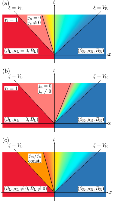
Figure 1: Schematic picture of partitioning protocol and nonequilibrium phenomena studied in this paper. (a) Charge clogged region, where $j_{n}=0$ and $j_{e}\neq 0$. (b) Stationary charge clogging. The region of $n=1$ includes $\xi=0$. (c) Proportionality of spin and charge currents when $\mu_{{\mathrm{L}}}\neq 0$ and $B_{{\mathrm{L}}}\neq 0$. The ratio $j_{m}/j_{n}$ is fixed to a constant value in a region to the right of $\xi=V_{{\mathrm{L}}}$. Outside the light cones, $\xi\leq V_{{\mathrm{L}}}$ or $\xi\geq V_{{\mathrm{R}}}$, local states are unchanged from the initial left or right thermal equilibrium states, respectively.

This paper is organized as follows. In Sec. II, we introduce the 1D Hubbard model and the GHD approach to it. In particular, we describe how to calculate the profiles of densities and currents for the partitioning protocol. In Sec. III, we present the main results on the expansion of a half-filled region. We show initial conditions where stationary charge clogging occurs and analyze the initial conditions dependence of the existence of it. We also examine stationary spin clogging. In Sec. IV, we present the main results on the proportionality of spin and charge currents at finite temperatures. To study the proportionality, we analyze the profiles of the ratio of spin current to particle density current and their initial conditions dependence. We also analyze the profiles of the ratio of energy current to particle density current. Finally, the conclusions are given in Sec. V.

II Model and Method

Let us briefly summarize in this section the GHD approach to the 1D Hubbard model PhysRevB.96.081118 ; PhysRevB.101.035121 . Throughout this paper, we will use the notations defined in our previous work (Ref. PhysRevB.101.035121, ). Refer to that paper for more details of the calculations.

The Hamiltonian of the 1D Hubbard model on $L$ sites reads as

$$\hat{H}= -\sum_{j=1}^{L}\sum_{\sigma}\left[\bigl{(}\hat{c}_{j,\sigma}^{\dagger}\hat{c}_{j+1,\sigma}+\mathrm{H.c.}\bigr{)}+(\mu+s_{\sigma}B)\hat{n}_{j,\sigma}\right]$$

$$+4u\sum_{j=1}^{L}\left[\bigl{(}\hat{n}_{j,\uparrow}-{\textstyle\frac{1}{2}}\bigr{)}\bigl{(}\hat{n}_{j,\downarrow}-{\textstyle\frac{1}{2}}\bigr{)}-{\textstyle\frac{1}{4}}\right],$$ (1)

where $\hat{c}_{j,\sigma}^{\dagger}$ and $\hat{c}_{j,\sigma}$ are the electron creation and annihilation operator, respectively, at site $j$ with spin $\sigma\ \in\{\uparrow,\downarrow\}$. $\hat{n}_{j,\sigma}\equiv\hat{c}^{\dagger}_{j,\sigma}\hat{c}_{j,\sigma}$ and $s_{\sigma}$ is defined as $s_{\uparrow}=1$ and $s_{\downarrow}=-1$. We set the electron hopping amplitude to be unity, and use it as the unit of energy throughout this paper. $\mu$ and $B$ are chemical potential and magnetic field, respectively. The Coulomb repulsion is parameterized by $u~{}>0$, and the constant $-1/4$ in this term is included so as to make the energy of the vacuum state zero.

The partitioning protocol is shown in Fig. 1. Initially, the system is divided into left and right parts, and they are independently thermalized with different sets of parameters ($\beta_{{\mathrm{L}}}$, $\mu_{{\mathrm{L}}}$, $B_{{\mathrm{L}}}$) and ($\beta_{{\mathrm{R}}}$, $\mu_{{\mathrm{R}}}$, $B_{{\mathrm{R}}}$). At time $t=0$, the two part are connected at the origin $x=0$, and we study the time evolution of the total system. The initial particle density $n^{{\mathrm{L}}({\mathrm{R}})}$, magnetization $m^{{\mathrm{L}}({\mathrm{R}})}$, and energy density $e^{{\mathrm{L}}({\mathrm{R}})}$ are controlled by the corresponding set of the parameters. Hereafter we consider the case of $\mu_{\mathrm{s}}\leq 0$ and $B_{\mathrm{s}}\geq 0$ for $\mathrm{s}={\mathrm{L}},{\mathrm{R}}$, which means $n^{{\mathrm{L}}({\mathrm{R}})}\leq 1$ and $m^{{\mathrm{L}}({\mathrm{R}})}\geq 0$.

The GHD theory describes a state by the distribution functions of quasiparticles $\left\{\rho_{a}(w;x,t)\right\}$, and the time evolution is defined by their continuity equations. Here, the integer label $a$ denotes the type of quasiparticles. The first type corresponding to $a=0$ is called real $k$. They are scattering states of polarized electrons, and each state carries the electron charge $e(<0)$ and spin projection $1/2$. The variable $w$ takes a real value $k$ and represents charge momentum $(-\pi<k\leq\pi)$. The second type corresponding to $a>0$ is called $\Lambda$-string. They are either scattering states of spins $(a=1)$ or bound states of spins $(a>1)$. Each state carries spin projection $-a$. In this case, the variable $w=\Lambda$ represents the real part of complex spin rapidity $(-\infty<\Lambda<\infty)$. The third type corresponding to $a<0$ is called $k$-$\Lambda$ string. They are bound states of charges, and each state carries charge $2|a|e$. The variable $w=\Lambda$ now represents the real part of complex charge rapidity.

The distribution functions evolve in time following the continuity equations PhysRevX.6.041065 ; PhysRevLett.117.207201 ; PhysRevLett.125.070602 $\frac{\partial}{\partial t}\,\rho_{a}\left(w;x,t\right)+\frac{\partial}{\partial x}\,\left[\accentset{\circ}{v}_{a}(w;x,t)\rho_{a}(w;x,t)\right]=0$. Here, $\{\accentset{\circ}{v}_{a}\}$ are the dressed velocities PhysRevLett.113.187203 , and the reader should refer to Refs. PhysRevB.96.081118, ; PhysRevB.101.035121, to know how to obtain them. Upon using the partitioning protocol, it is known that the solution of the continuity equations only depends on the ray $\xi\equiv x/t$, and it is convenient to introduce the filling functions $\left\{\vartheta_{a}(w;\xi)\right\}$ to represent the solution PhysRevX.6.041065 ; PhysRevLett.117.207201 . Once $\left\{\vartheta_{a}(w;\xi)\right\}$ are obtained, the distribution functions $\left\{\rho_{a}(w;\xi)\right\}$ are calculated by solving the integral equations called the Takahashi equations 10.1143/PTP.47.69 . The solution of the filling functions are written as

$$\vartheta_{a}(w,\xi)=~{}\Theta\left(\accentset{\circ}{v}_{a}(w,\xi)-\xi\right)\vartheta_{a}^{{\mathrm{L}}}(w)+\Theta\left(\xi-\accentset{\circ}{v}_{a}(w,\xi)\right)\vartheta_{a}^{{\mathrm{R}}}(w)$$ (2)

with Heaviside’s step function $\Theta(x)$. $\{\vartheta_{a}^{{\mathrm{L}}({\mathrm{R}})}(w)\}$ are the initial left (right) filling functions and obtained by solving the integral equations for thermal equilibrium specified by the set of parameters $(\beta_{{\mathrm{L}}({\mathrm{R}})},\mu_{{\mathrm{L}}({\mathrm{R}})},B_{{\mathrm{L}}({\mathrm{R}})})$, which are called the thermodynamic Bethe ansatz (TBA) equations 10.1143/PTP.47.69 . We note that the dressed velocities depend on the filling functions and therefore both of them have to be determined self-consistently. The above solution shows that the value of $\vartheta_{a}(w,\xi)$ is identical to its initial value either in the left or right part.

Once the distribution functions $\left\{\rho_{a}(w;\xi)\right\}$ and the dressed velocities $\{\accentset{\circ}{v}_{a}(w,\xi)\}$ are obtained, they suffice to calculate densities and currents. The particle density $n$, magnetization $m$, and energy density $e$ and their currents $j_{n}$, $j_{m}$, $j_{e}$ are given by PhysRevB.96.081118

$$\left[\begin{array}[]{c}\displaystyle n_{r}(\xi)\\[4.0pt] \displaystyle j_{r}(\xi)\end{array}\right]=\sum_{a}\int dw\,\left[\begin{array}[]{c}\displaystyle 1\\[4.0pt] \displaystyle\accentset{\circ}{v}_{a}(w,\xi)\end{array}\right]f_{r,a}(w)\rho_{a}(w,\xi),$$ (3)

where the label ($r=n,m,e$) distinguishes densities $n_{n}=n$, $n_{m}=m$, and $n_{e}=e$ and corresponding currents. The weights are defined as

$$f_{n,a}(w) =\delta_{a,0}+|a|-a,$$ (4)

$$f_{m,a}(w) ={\textstyle\frac{1}{2}}\left(\delta_{a,0}-|a|-a\right),$$ (5)

$$f_{e,a}(w) =e_{a}(w).$$ (6)

Here, $e_{a}$ is the bare energy of the type-$a$ quasiparticle:

$$e_{0}(k) =-2\cos k-2u,$$

$$e_{a<0}(\Lambda) =4\operatorname{Re}\sqrt{1-(\Lambda+iau)^{2}}+4au,$$ (7)

and $e_{a>0}(\Lambda)=0$. The symbol $\operatorname{Re}$ denotes the real part.

We define light cones $\xi_{a}^{\pm}$ for each string $a$ for later use. From Eq. (2), $\xi_{a}^{\pm}$ are defined as the minimum and maximum $\xi$-values on the intersection line of the two surfaces $z_{1}(w,\xi)=\accentset{\circ}{v}_{a}(w,\xi)$ and $z_{2}(w,\xi)=\xi$. The filling function $\vartheta_{a}(w,\xi)$ continuously varies inside the light cone $\xi_{a}^{-}<\xi<\xi_{a}^{+}$, while outside the light cone it is fixed to either $\vartheta_{a}^{{\mathrm{L}}}(w)$ or $\vartheta_{a}^{{\mathrm{R}}}(w)$. In addition, we also define

$$V_{{\mathrm{L}}} \equiv\min_{a}\xi_{a}^{-}=\xi_{0}^{-}, V_{{\mathrm{R}}} \equiv\max_{a}\xi_{a}^{+}=\xi_{0}^{+},$$

$$V_{{\mathrm{L}},1} \equiv\min_{a\neq 0}\xi_{a}^{-}, V_{{\mathrm{R}},1} \equiv\max_{a\neq 0}\xi_{a}^{+},$$ (8)

and the first two are determined by real $k$ quasiparticles. The definition means that all the filling functions are equal to the initial equilibrium values in the left part at $\xi\leq V_{{\mathrm{L}}}$, while those in the right part at $\xi\geq V_{{\mathrm{R}}}$. We note that $V_{{\mathrm{L}}}$ does not depend on $(\beta_{{\mathrm{R}}},\mu_{{\mathrm{R}}},B_{{\mathrm{R}}})$, and vice versa. In the regions $V_{{\mathrm{L}}}\leq\xi\leq V_{{\mathrm{L}},1}$ and $V_{{\mathrm{R}},1}\leq\xi\leq V_{{\mathrm{R}}}$, only real-$k$ quasiparticles have a filling function different from the initial equilibrium values.

Throughout this paper we set the repulsion $u=2$. Approximations used for the numerical calculations at finite temperatures are the same as in our previous work PhysRevB.101.035121 , where the cut-off concerning the number of integral equations $a_{c}$ is used PhysRevB.65.165104 . The values of the densities and currents shown in figures are extrapolated ones obtained from the calculations for $a_{c}=36,42,\text{and}~{}48$.

III Stationary clogging

When the initial left state is set half-filling ($\mu_{{\mathrm{L}}}=0$) at infinite or high temperatures, there emerges a charge clogged region near the left end of the intermediate transient region

$$n(\xi)=1,\ j_{n}(\xi)=0,\ j_{e}(\xi)\not\equiv 0,\quad\bigl{(}V_{{\mathrm{L}}}<{}^{\forall}\xi<\xi_{-\infty}^{-}\bigr{)}.$$ (9)

In our previous work PhysRevB.101.035121 , the initial right state was an electron vacuum, and then $\xi_{-\infty}^{-}<0$ for all the parameters examined. Therefore, the clogging phenomenon appears only at sites in the left half, and also it continues only for a limited time, which is proportional to the distance between the site position and the origin.

We now examine if one can realize clogging in a stationary state by tuning initial conditions. Stationary values of physical quantities are those at $\xi=0$, and therefore the question is how to tune parameters for achieving $\xi_{-\infty}^{-}>0$. We will show that a key point is the density of real-$k$ quasiparticles, $n_{0}(\xi)$. In all the cases in this section, we will control the initial conditions in the right part, while the initial left state is prepared with $\beta_{{\mathrm{L}}}=0.5$ and fixed at half-filling $\mu_{{\mathrm{L}}}=0$ except for the data in Fig. 8.

Let us first set the initial temperature in the right part lower than the left part $\beta_{{\mathrm{R}}}=2$, and control chemical potential in the range of $-5\leq\mu_{{\mathrm{R}}}\leq-1$. Magnetic field is set zero in both parts $B_{{\mathrm{L}}}=B_{{\mathrm{R}}}=0$. Figure 2 shows the profiles of particle density $n(\xi)$ and its current $j_{n}(\xi)$. One should recall that $V_{{\mathrm{L}}}\approx-2.0$ does not depend on $\mu_{{\mathrm{R}}}$. The figure shows a clogging phenomenon for all $\mu_{{\mathrm{R}}}$’s and the particle density is fixed to 1 in the clogging region. Its right end $\xi^{-}_{-\infty}$ moves to the right with increasing $\mu_{{\mathrm{R}}}$, and the clogging region includes $\xi=0$ for the two largest values $\mu_{{\mathrm{L}}}=-2$ and $-1$. Thus, charge clogging occurs in the stationary state in these cases.

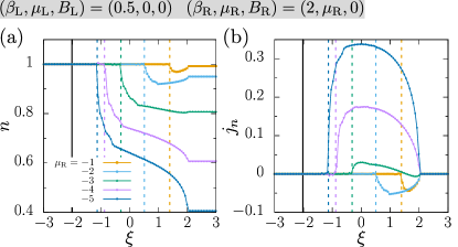
Figure 2: Profiles of (a) particle density $n(\xi)$ and (b) its current $j_{n}(\xi)$ for various values of $\mu_{{\mathrm{R}}}$. Vertical dashed and solid lines are $\xi^{-}_{-\infty}$ and $V_{{\mathrm{L}}}$, which are the borders of charge clogged region.

Stationary clogging is accompanied by another interesting phenomenon, and that is back current. Figure 2(b) shows a region where $j_{n}<0$ for $\mu_{{\mathrm{L}}}=-2$ and $-1$, namely particle density current flows towards the high-density region. This is related to a nonmonotonic behavior of $n(\xi)$ in Fig. 2(a). One can explain the presence of back current based on the continuity equation of particle density $\xi\partial_{\xi}n(\xi)=\partial_{\xi}j_{n}(\xi)$. Integrating this over the region $V_{{\mathrm{L}}}\leq\xi\leq V_{{\mathrm{R}}}$ with the boundary values $j_{n}(V_{{\mathrm{L}}})=j_{n}(V_{{\mathrm{R}}})=0$, one obtains

$$0=\int_{V_{{\mathrm{L}}}}^{V_{{\mathrm{R}}}}d\xi\partial_{\xi}j_{n}(\xi)=\int_{V_{{\mathrm{L}}}}^{V_{{\mathrm{R}}}}d\xi\xi\partial_{\xi}n(\xi).$$ (10)

If the clogged region extends beyond $\xi=0$, then $n(\xi)=1$ for ${}^{\forall}\xi\leq 0$, and the above integral is rewritten as

$$0=\int_{0}^{V_{{\mathrm{R}}}}d\xi\xi\partial_{\xi}n(\xi)=-\int_{0}^{V_{{\mathrm{R}}}}d\xi\delta n(\xi),$$ (11)

where $\delta n(\xi)\equiv n(\xi)-n^{{\mathrm{R}}}$ is density deviation. Since $\delta n(\xi\approx 0)>0$, this integral means that there exists a finite-width region where $\delta n(\xi)<0$. At the right end, $\delta n(V^{{\mathrm{R}}})=0$, and thus $n(\xi)$ should be nonmonotonic. Let us also examine particle current density. Just above $\xi^{-}_{-\infty}>0$, $\partial_{\xi}n$ is negative, and this leads to

$$j_{n}(\xi)=\int_{\xi^{-}_{-\infty}}^{\xi}d\xi^{\prime}\,\xi^{\prime}\,\partial_{\xi^{\prime}}n(\xi^{\prime})<0,$$ (12)

at least if $0<\xi-\xi^{-}_{-\infty}\ll 1$. Therefore, although the left part initially has a higher density of electrons, the particle current flows to the left in this region. This contrasts with the ordinary current flow driven by particle diffusion and may be called back current in this sense.

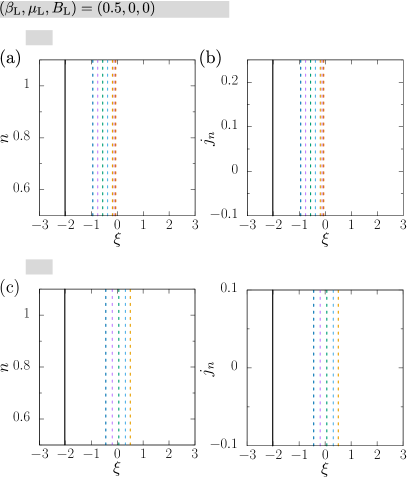
Figure 3: Effect of magnetic field in the right initial state $B_{{\mathrm{R}}}$ on the profiles of $n(\xi)$ and $j_{n}(\xi)$. (a), (b) $B_{{\mathrm{R}}}=0$ and $-5\leq\mu_{{\mathrm{R}}}\leq-0.25$, while (c), (d) $B_{{\mathrm{R}}}=4$ and $-5\leq\mu_{{\mathrm{R}}}\leq-1$.

We next consider the case of controlling $\mu_{{\mathrm{R}}}$ when the initial temperature is identical in both parts $\beta_{{\mathrm{L}}}=\beta_{{\mathrm{R}}}=0.5$. As in the previous case, $\mu_{{\mathrm{L}}}=0$ and $B_{{\mathrm{L}}}=0$. Figures 3(a) and 3(b) show $n(\xi)$ and $j_{n}(\xi)$ at $B_{{\mathrm{R}}}=0$ for $-5\leq\mu_{{\mathrm{R}}}\leq-0.25$. Since $\xi^{-}_{-\infty}<0$ for all $\mu_{{\mathrm{R}}}$’s, stationary charge clogging does not occur, and we try another type of control, i.e., applying magnetic field. Figures 3(c) and 3(d) show $n(\xi)$ and $j_{n}(\xi)$ at $B_{{\mathrm{R}}}=4$ for $-5\leq\mu_{{\mathrm{R}}}\leq-1$. The other initial conditions are the same as those in Figs. 3(a) and 3(b). The result is that stationary charge clogging occurs for $\mu_{{\mathrm{R}}}\geq-3$.

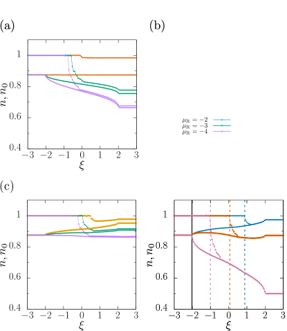
Figure 4: Real-$k$ quasiparticle density $n_{0}(\xi)$ and total electron density $n(\xi)$ for four different parameter sets of the right initial state [(a), (b), (c), and (d)]. Panel (d) also shows $V_{{\mathrm{L}}}$ (solid line) and $\xi^{-}_{-\infty}$ (dashed lines).

Figures 2 and 3 show that stationary charge clogging occurs when the initial right state is prepared either at low temperature or in a large magnetic field. We examined the main effect of these initial conditions and found that one common effect is the high density of real-$k$ quasiparticle excitations $n^{{\mathrm{R}}}_{0}$. This is because the real-$k$ excitations have an energy lower than charge bound states ($k$-$\Lambda$ string) and have spin $1/2$, while $k$-$\Lambda$ string carries spin $0$. Therefore, real-$k$ excitations have a higher density at lower temperature, and they are more susceptible to magnetic field.

To study this point systematically, we fix the left initial state and vary $\mu_{{\mathrm{R}}}$ to check stationary clogging for each $(\beta_{{\mathrm{R}}},B_{{\mathrm{R}}})$ of four choices. Figure 4 shows the calculated profiles of $n(\xi)$ and $n_{0}(\xi)$. The initial left state is the same one as in Figs. 2 and 3: $(\beta_{{\mathrm{L}}},\mu_{{\mathrm{L}}},B_{{\mathrm{L}}})=(0.5,0,0)$. In this case, $n^{{\mathrm{L}}}=1$ and $n^{{\mathrm{L}}}_{0}\approx 0.875$. The four sets of $(\beta_{{\mathrm{R}}},B_{{\mathrm{R}}})$ are also the same as those in Figs. 2 and 3 except for the set $(2,4)$. The results show that stationary charge clogging for all the $(\beta_{{\mathrm{R}}},B_{{\mathrm{R}}})$ sets except $(0.5,0)$ when $|\mu_{{\mathrm{R}}}|$ is small.

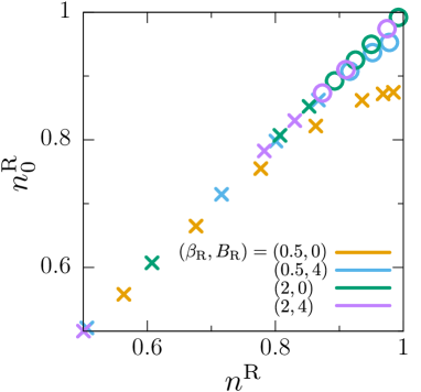
Figure 5: The real-$k$ quasiparticle density $n_{0}^{{\mathrm{R}}}$ plotted versus the total density $n^{{\mathrm{R}}}$ in the initial right state. $\mu_{{\mathrm{R}}}$ is varied in the range $-8\leq\mu_{{\mathrm{R}}}\leq-0.25$ for each set of $(\beta_{{\mathrm{R}}},B_{{\mathrm{R}}})$. Circles show that stationary charge clogging occurs, while crosses show no clogging.

Let us first examine how stationary charge clogging correlates with the total electron density $n^{{\mathrm{R}}}$ and real-$k$ quasiparticle density $n_{0}^{{\mathrm{R}}}$ in the initial right state. Figure 5 shows $n_{0}^{{\mathrm{R}}}$ and $n^{{\mathrm{R}}}$ and also shows whether stationary charge clogging occurs. The cases that stationary charge clogging occurs are shown by a circle symbol. The parameters $(\beta_{{\mathrm{R}}},B_{{\mathrm{R}}})$ for the right initial state are identical to those used in Fig. 4, but a larger number of $\mu_{{\mathrm{R}}}$ values are used. This plot shows that the most important factor for realizing stationary charge clogging is a high density of $n_{0}^{{\mathrm{R}}}$. As shown by the results for $(\beta_{{\mathrm{R}}},B_{{\mathrm{R}}})=(0.5,0)$, the total density $n^{{\mathrm{R}}}$ is large but stationary clogging does not occur. Therefore, $n^{{\mathrm{R}}}$ is not a primary factor to determine the appearance of stationary charge clogging.

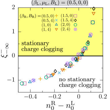
Figure 6: Right border of charge clogged region $\xi_{-\infty}^{-}$ plotted versus the density difference of real-$k$ quasiparticles between the two initial states $n_{0}^{{\mathrm{R}}}-n_{0}^{{\mathrm{L}}}$. The part of $\xi_{-\infty}^{-}>0$ is the region of stationary charge clogging.

We confirm this expectation that stationary charge clogging is determined the density of real-$k$ quasiparticles. Figure 6 shows the right border of charge clogged region $\xi_{-\infty}^{-}$ plotted versus $n_{0}^{{\mathrm{R}}}-n_{0}^{{\mathrm{L}}}$. The data are calculated for the same sets of initial conditions as in Fig. 5 and supplemented by the results at intermediate temperatures $(\beta_{{\mathrm{R}}},B_{{\mathrm{R}}})=(1,0)$, $(1,4)$, $(1.5,0)$, and $(1.5,4)$. The part of $\xi_{-\infty}^{-}>0$ corresponds to the cases of stationary charge clogging, and this agrees precisely with the region of $n_{0}^{{\mathrm{R}}}-n_{0}^{{\mathrm{L}}}>0$. The results show a universal curve for the different sets of data, and this means that the right border $\xi_{-\infty}^{-}$ is determined by the one factor $n_{0}^{{\mathrm{R}}}-n_{0}^{{\mathrm{L}}}>0$ alone, at least when the initial left state is fixed. Therefore, although this analysis is based on numerical calculations with eight parameter sets, it is likely that this is a general criterion for realizing stationary charge clogging, represented explicitly as

$$(n^{{\mathrm{L}}}-n^{{\mathrm{R}}})(n_{0}^{{\mathrm{L}}}-n_{0}^{{\mathrm{R}}})<0,\mbox{~{}and~{}}(1-n^{{\mathrm{L}}})(1-n^{{\mathrm{R}}})=0,$$ (13)

where the latter condition is equivalent to $\mu_{{\mathrm{L}}}=0$ or $\mu_{{\mathrm{R}}}=0$. Namely, the majority-minority relation should be reversed between the total electron density and the density of real-$k$ quasiparticles.

We also examine the possibility of stationary spin clogging. This occurs when $B_{{\mathrm{L}}}=0$ and is characterized as

$$m(\xi)=0,\ j_{m}(\xi)=0,\ j_{e}(\xi)\not\equiv 0,\quad\bigl{(}V_{{\mathrm{L}}}<{}^{\forall}\xi<\xi_{\infty}^{-}\bigr{)},$$ (14)

while $m\not\equiv 0$, $j_{m}\not\equiv 0$ at $\xi_{\infty}^{-}<\xi<V_{{\mathrm{R}}}$. Figure 7 shows the profiles of magnetization $m(\xi)$ and spin current $j_{m}(\xi)$ for $-10\leq\mu_{{\mathrm{R}}}\leq-5$. The two sets of initial conditions are those used in Figs. 3 and 4, and $\beta_{{\mathrm{R}}}$ is different between the two. The right boundary of spin clogged region is $\xi^{-}_{\infty}$ not $\xi^{-}_{-\infty}$, and it is shown by dashed lines. For both sets of initial conditions, stationary spin clogging occurs for $\mu_{{\mathrm{R}}}\leq-8$. In contrast to charge clogging, stationary spin clogging occurs when $|\mu_{{\mathrm{R}}}|$ is large, i.e., $n^{{\mathrm{R}}}$ is small. Similar to stationary charge clogging, we numerically confirmed that stationary spin clogging occurs, if the following criterion is satisfied

$$(m^{{\mathrm{L}}}-m^{{\mathrm{R}}})(m_{0}^{{\mathrm{L}}}-m_{0}^{{\mathrm{R}}})<0,\mbox{~{}and~{}}m^{{\mathrm{L}}}m^{{\mathrm{R}}}=0.$$ (15)

For all the initial conditions used, we never found the coexistence of charge and spin cloggings in the stationary state.

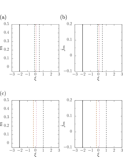
Figure 7: Profiles of (a), (c) magnetization density $m(\xi)$ and (b), (d) spin current $j_{m}(\xi)$ for various values of chemical potential in the right initial state $\mu_{{\mathrm{R}}}$. Vertical solid and dashed lines represent $V_{{\mathrm{L}}}$ and $\xi^{-}_{\infty}$, which are the borders of spin clogged region. In (c) and (d), $\xi^{-}_{\infty}$’s for $\mu_{{\mathrm{R}}}=-5$ and $\mu_{{\mathrm{R}}}=-6$ overlap.

Finally, we note that back current is not limited to the case when stationary charge clogging occurs. Figure 8 shows an example in the case of $(\beta_{{\mathrm{L}}},\mu_{{\mathrm{L}}},B_{{\mathrm{L}}})=(0.5,-0.25,0)$ and $(\beta_{{\mathrm{R}}},\mu_{{\mathrm{R}}},B_{{\mathrm{R}}})=(2,-5,4)$. In this case, $n^{{\mathrm{L}}}\approx 0.984>n^{{\mathrm{R}}}\approx 0.974\approx n_{0}^{{\mathrm{R}}}>n_{0}^{{\mathrm{L}}}\approx 0.875$. Both initial states are prepared with nonzero chemical potential, and stationary charge clogging does not occur. However, Fig. 8(b) shows that back current ($j_{n}<0$) flows. As in the cases of stationary charge clogging, $n(\xi)$ is not monotonic while $n_{0}(\xi)$ is monotonic. In the region $V_{{\mathrm{L}}}<\xi<\xi_{-\infty}^{-}$, $n(\xi)$ increases slightly with $\xi$ and approaches toward half filling. The current $j_{n}(\xi)$ is nonzero but its amplitude is small. In this sense, this is a “pseudo clogged” region. For $\xi>\xi_{-\infty}^{-}$, $n(\xi)$ decreases quickly and this is accompanied by a large enhancement of $j_{n}$. This decrease stops at $\xi=V_{{\mathrm{R}},1}=\xi_{-1}^{+}$ and then $n(\xi)$ increases again.

It is notable that back current extends over the entire transient region $V_{{\mathrm{L}}}<\xi<V_{{\mathrm{R}}}$. Therefore, the stationary particle density $n(0)$ is larger than the initial particle densities in both left and right parts $n(0)>\max\{n^{{\mathrm{R}}},n^{{\mathrm{L}}}\}$ as shown in Fig. 8(a). One should note that the back current is attributed to real-$k$ quasiparticle current $j_{n,0}<0$, and all the contributions of bound state excitations show a normal behavior, i.e., flows towards lower-density side $j_{n,a}>0$ for $a<0$.

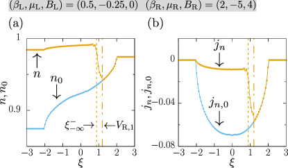
Figure 8: Profiles of (a) particle density $n(\xi)$ and (b) its current $j_{n}(\xi)$ when back current flows without charge clogging.

IV Proportionality of currents

In this section, we investigate the relations, particularly proportionality, among spin, charge, and energy currents. As will be shown later, there exist several $\xi$-regions showing different behaviors of current ratios. To realize nonzero spin current as well as charge current, we use initial conditions that nonzero magnetic field and chemical potential are applied to the left initial state: $\bar{\mu}\equiv\beta_{{\mathrm{L}}}\mu_{{\mathrm{L}}}\neq 0$ and $\bar{B}\equiv\beta_{{\mathrm{L}}}B_{{\mathrm{L}}}\neq 0$. In our previous work PhysRevB.101.035121 , we studied the ratio of spin and charge currents in the high-temperature limit $\beta_{{\mathrm{L}}}=0$ and showed that the following simple relation holds in a region connected to the left thermal equilibrium

$$\frac{j_{m}\left(\xi\right)}{j_{n}\left(\xi\right)}=\frac{\tanh\bar{B}}{2\tanh|\bar{\mu}|},\ \ \ (\beta_{{\mathrm{L}}}\rightarrow 0,\ V_{{\mathrm{L}}}<\xi<V_{{\mathrm{L}},1}),$$ (16)

where $V_{{\mathrm{L}},1}$ is defined in Eq. (8).

Let us first investigate how nonzero $\beta_{{\mathrm{L}}}$ changes this proportionality. Figure 9 shows the spatial profiles of the current ratio $j_{m}(\xi)/j_{n}(\xi)$ and the corresponding density ratio $m(\xi)/n(\xi)$ for various values of $\beta_{{\mathrm{L}}}$ whereas $(\bar{\mu},\bar{B})$ is fixed to one of four pairs. Note that $\mu_{{\mathrm{L}}}$ and $B_{{\mathrm{L}}}$ are also varied simultaneously to fix $(\bar{\mu},\bar{B})$. The initial right state is set so that $n^{{\mathrm{R}}}=0$. All the data in Figs. 9(a)-9(d) show a plateau behavior of $j_{m}(\xi)/j_{n}(\xi)$. Namely, the region of constant current ratio persists for all $\beta_{{\mathrm{L}}}>0$’s used and its width agrees quite well with $V_{{\mathrm{L}}}<\xi<V_{{\mathrm{L}},1}$ calculated for each $\beta_{{\mathrm{L}}}$. For $\xi>V_{{\mathrm{L}},1}$, the current ratio decreases with $\xi$, but shows a second plateau for larger $\xi$, which will be discussed later in detail. Varying $\beta_{{\mathrm{L}}}$ at least in the high-temperature region does not destroy a plateau in the current ratio but has two main effects. The first effect is about the constant ratio of $j_{m}/j_{n}$. Lowering temperature with keeping $(\bar{\mu},\bar{B})$ fixed decreases its value from the high-temperature limit (16), which is shown by the black solid line in each panel of the figure. The second effect is about the width of the first plateau, and lowering temperature shrinks its width. Comparison of the data for the different sets of $(\bar{\mu},\bar{B})$ shows that larger $|\mu_{{\mathrm{L}}}|$ or smaller $|B_{{\mathrm{L}}}|$ expands the plateau width when $\beta_{{\mathrm{L}}}$ is fixed.

It is important that the plateau value of the current ratio $j_{m}/j_{n}$ differs from the corresponding density ratio $m(\xi)/n(\xi)$, which changes with $\xi$ in this region, and also from the ratio in the left equilibrium state $m^{{\mathrm{L}}}/n^{{\mathrm{L}}}$. This is consistent with the fact that these ratios differ from Eq. (16) in the high-temperature limit PhysRevB.101.035121 ; 10.1143/PTP.47.69 :

$$\frac{m(\xi)}{n(\xi)} =\frac{\tanh\bar{B}}{2\tanh|\bar{\mu}|}\left[1-\frac{2n(\xi)^{-1}}{e^{2|\bar{\mu}|}+1}\right],\ \ \ (V_{{\mathrm{L}}}<\xi<V_{{\mathrm{L}},1}),$$ (17)

$$\frac{m^{{\mathrm{L}}}}{n^{{\mathrm{L}}}} =\frac{\sinh\bar{B}}{2(e^{-|\bar{\mu}|}+\cosh\bar{B})}.$$ (18)

The current and density ratios, $j_{m}/j_{n}$ and $m/n$, become closer with further increasing $\xi>V_{{\mathrm{L}},1}$.

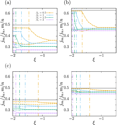
Figure 9: Profiles of the current ratio $j_{m}(\xi)/j_{n}(\xi)$ (solid lines) and the corresponding density ratio $m(\xi)/n(\xi)$ (dashed lines). In each panel [(a), (b), (c), and (d)], the temperature in the initial left state is varied in the range $0.5\leq\beta_{{\mathrm{L}}}\leq 2$, while the pair $(\beta_{{\mathrm{L}}}\mu_{{\mathrm{L}}},\beta_{{\mathrm{L}}}B_{{\mathrm{L}}})$ is fixed. The initial right state is an electron vacuum $n^{{\mathrm{R}}}=0$. Vertical dashed-dotted line shows $V_{{\mathrm{L}},1}$, while horizontal black solid line represents the high-temperature limit (16).

We next examine how the right initial state changes the proportionality among $j_{n}$, $j_{m}$, and energy current $j_{e}$. Figure 10 shows the results for the two values of temperature, $\beta_{{\mathrm{R}}}=0.5$ and 2. For each value, chemical potential is varied in the range $-\infty\leq\mu_{R}\leq-3$, and the upper two panels show the proportionality between $j_{m}$ and $j_{n}$, while the lower two are for $j_{e}$ and $j_{n}$. The other parameters of the initial condition are set to the same values used in Fig. 9(b): $(\beta_{{\mathrm{L}}},\mu_{{\mathrm{L}}},B_{{\mathrm{L}}})=(1,-1,2)$ and $B_{{\mathrm{R}}}=0$.

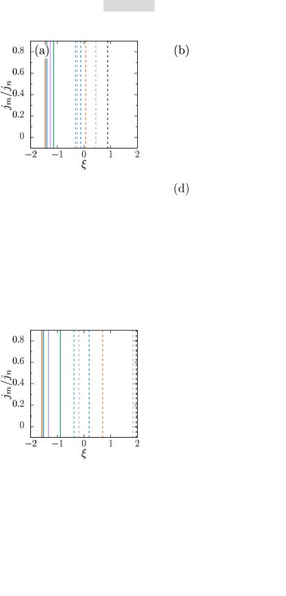
Figure 10: Effects of varying the initial right conditions on the profiles of the ratios (a), (e) $j_{m}/j_{n}$ and (c), (g) $j_{e}/j_{n}$. Characteristics are also shown for (b), (f) $j_{n}$-$j_{m}$ and (d), (h) $j_{n}$-$j_{e}$. In panels (a) and (e), vertical solid lines represent $\xi_{-1}^{+}$, and vertical dashed lines represent $\xi_{1}^{-}$.

Let us discuss the results in Fig. 10. Figures 10(a) and 10(e) show that the ratio $j_{m}/j_{n}$ in the first plateau region $V_{{\mathrm{L}}}<\xi<V_{{\mathrm{L}},1}$ hardly depends on the initial right conditions $j_{m}/j_{n}\approx 0.62$. This is also reflected by a universal slope of the lines starting from the origin in Figs. 10(b) and 10(f). In all of these cases, $V_{{\mathrm{L}},1}=\xi_{-1}^{-}$, and this means that the right boundary of the current ratio plateau is characterized by the left light cone of the charge bound state with $a=-1$. Thus, quasiparticles with charge $2e$ break the constant current ratio.

Another interesting finding is that the current ratio $j_{m}/j_{n}$ shows a second plateau around $\xi\sim-1$ in Figs. 10 (a) and (e). The $j_{m}$-$j_{n}$ curves in the panels (b) and (f) show this second plateau as an almost straight inclined line in the most distant part from the origin. The current ratio in the second plateau is smaller than the value in the first plateau. In contrast to the first plateau, this value depends on the initial condition $\mu_{{\mathrm{R}}}$ in the right part, and this is particularly evident at $\beta_{{\mathrm{R}}}=0.5$. The ratio increases as $\mu_{{\mathrm{R}}}$ approaches zero, and this control corresponds to varying $n_{{\mathrm{R}}}$ towards $n_{{\mathrm{L}}}$. We found that the left border of the second plateau is determined by the light cone $\xi_{-1}^{+}$. Its value is calculated for each $\mu_{{\mathrm{R}}}$ and shown by a solid line in the figure ($-6\leq\mu_{{\mathrm{R}}}\leq-3$ for visibility). The right border is the light cone $\xi_{1}^{-}$ and shown by a dashed line. It is interesting that the second plateau expands as $\mu_{{\mathrm{R}}}$ goes down ($n_{{\mathrm{R}}}$ decreases). This is related to the size of spin clogged region, which will be explained below.

With further increasing $\xi$, the second plateau terminates and the current ratio $j_{m}/j_{n}$ shows a continuous drop down to 0. This part is represented in the $j_{m}$-$j_{n}$ curves as a vertical edge of each triangular loop.

The rightmost part connected to the right initial state is a spin clogged region, where $j_{m}/j_{n}=0$. This is dual to charge clogged region, which appears when the two parts with $\mu=0$ and $\neq 0$ are connected. In this case, the two parts with $B=0$ and $\neq 0$ are connected and a spin clogged region appears. The spin clogged region corresponds to a base of each $j_{m}$-$j_{n}$ loop. Its width is determined by $V^{{\mathrm{R}}}-\xi_{\infty}^{+}$ and expands as $\mu_{{\mathrm{R}}}$ goes up (i.e., higher density of $n_{{\mathrm{R}}}$).

Thus, summarizing the behavior of the current ratio $j_{m}/j_{n}$, the whole transient space $V_{{\mathrm{L}}}<\xi<V_{{\mathrm{R}}}$ is divided into five regions as shown in Fig. 11: two plateaus and one spin clogged regions separated by two transient regions. This is different when considering the ratio of energy and charge currents $j_{e}/j_{n}$.

Figure 10 also shows the proportionality between energy and particle density currents. Figures 10(c) and 10(g) show that the ratio $j_{e}/j_{n}$ changes with $\xi$ and its value also varies with the initial right conditions in the $\xi$-region of the first plateau of $j_{m}/j_{n}$. However, as $\xi$ approaches $V_{{\mathrm{L}}}$, the ratio $j_{e}/j_{n}$ approaches a universal value $\sim-5.2$. This value is independent of the initial right conditions. We calculated the ratio for other initial conditions and found that it depends on the initial left conditions. This result means that near the left thermal equilibrium state each carrier in particle density current also carries the identical energy irrespective of the initial right conditions.

For $\xi>V_{{\mathrm{L}},1}$, the ratio $j_{e}/j_{n}$ shows a large $\xi$ dependence for a while, but Figure 10(c) shows that $\xi$-dependence is strongly suppressed in the region of the second plateau of $j_{m}/j_{n}$ and also at other $\xi<V_{{\mathrm{R}}}$. This quasi-plateau behavior becomes more evident as $\mu_{{\mathrm{R}}}$ decreases, and the $j_{e}$-$j_{n}$ curve shows a retracing straight line in Fig. 10(d). The corresponding results for the case of lower temperature in the initial right state $\beta_{{\mathrm{R}}}=2$ are plotted in Figs. 10(g) and 10(h). In this case, the ratio $j_{e}/j_{n}$ shows a large $\xi$ dependence in the whole $\xi$ space, particularly for $\mu_{{\mathrm{R}}}=-3$ and $-4$, but the amplitude of both currents is quite small in those cases as shown in Fig. 10(h). Decreasing $\mu_{{\mathrm{R}}}$ below $-4$, the $\xi$-dependence in the region $\xi>-1.5$ is suppressed as in the case of $\beta_{{\mathrm{R}}}=0.5$, and the $j_{e}$-$j_{n}$ curve shows a quite straight path in Fig. 10(h). With decreasing $\mu_{{\mathrm{R}}}$, the ratio $j_{e}/j_{n}$ converges $-4$ in the quasi-plateau region. This value corresponds to the energy of a carrier with the fastest velocity $\max_{k}\accentset{\circ}{v}_{0}^{{\mathrm{R}}}(k)=\accentset{\circ}{v}_{0}^{{\mathrm{R}}}(\pi/2)=2$. As shown in Eq. (7), that is $e_{0}(\pi/2)=-2u=-4$, since $u=2$ in the present work.

Thus, summarizing the behavior of the ratio $j_{e}/j_{n}$, the whole transient space $V_{{\mathrm{L}}}<\xi<V_{{\mathrm{R}}}$ is now divided into three regions as shown in Fig. 11. In the first plateau and the first transient regions of $j_{m}/j_{n}$, the ratio $j_{e}(\xi)/j_{n}(\xi)$ shows a small and large dependence on $\xi$, respectively. In the remaining region, the ratio $j_{e}(\xi)/j_{n}(\xi)$ shows a quasi-plateau behavior that becomes evident as $\mu_{{\mathrm{R}}}$ decreases.

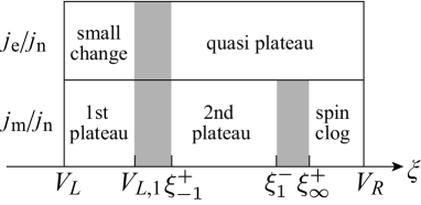
Figure 11: Summary of the behavior of the current ratios $j_{m}(\xi)/j_{n}(\xi)$ and $j_{e}(\xi)/j_{n}(\xi)$, for the initial conditions with $\mu_{{\mathrm{L}}}\neq 0$, $B_{{\mathrm{L}}}\neq 0$, and $B_{{\mathrm{R}}}=0$. Shaded parts are transient regions where the current ratio shows a large change.

V Conclusions

In this paper, we mainly studied two issues of the nonequilibrium quench dynamics in the 1D Hubbard model based on the generalized hydrodynamics theory with the partitioning protocol.

The first issue is the possibility of charge and spin clogging in a stationary state, i.e., the phenomenon where charge or spin current is zero whereas nonvanishing energy current flows at the ray $\xi=x/t=0$. We examined various cases of initial conditions under the constraint that the initial particle density is $n^{{\mathrm{L}}}=1$ and $n^{{\mathrm{R}}}<1$ for the two parts.

When stationary charge clogging occurs, the half-filled region expands to the right side. In Sec. III, we numerically solved the GHD equations for various initial conditions and found several cases of stationary charge and spin clogging. We studied the dependence on the initial conditions and found that an important factor is the particle density of scattering states $n_{0}$. We found by numerical calculations that the condition $n_{0}^{{\mathrm{L}}}<n_{0}^{{\mathrm{R}}}$ is crucial for stationary charge clogging [more precise one in Eq. (13)]. Similar to stationary charge clogging, when stationary spin clogging occurs, $m_{0}^{{\mathrm{L}}}-m_{0}^{{\mathrm{R}}}>0$ is satisfied in the cases of $m^{{\mathrm{L}}}=0$ and $m^{{\mathrm{R}}}>0$. When stationary charge clogging occurs, $n(\xi)$ should be nonmonotonic, and we found that there exists a back current, which flows towards the higher-density region ($n=1$). In the right part, as time goes, the particle density decreases first and then increases to be half filling, while the sign of its current does not change $j_{n}<0$.

The second issue is the proportionality among currents of spin $j_{m}$, charge $j_{n}$, and energy $j_{e}$. The current ratio $j_{m}/j_{n}$ in the high-temperature limit $\beta_{{\mathrm{L}}}=0$ was studied in our previous work PhysRevB.101.035121 . We numerically studied this issue at finite temperatures in Sec. IV and calculated the profiles of spin, particle density (equivalent to charge), and energy currents for various sets of initial conditions and analyzed the results. We found that the constant proportionality of $j_{m}$ and $j_{n}$ in the region $V_{{\mathrm{L}}}<\xi<V_{{\mathrm{L}},1}$ persists even at finite temperatures (the first plateau). The value of this constant ratio depends on the initial left temperature $\beta_{{\mathrm{L}}}$, but its dependence on the initial right conditions is negligible. Another finding is a second plateau of $j_{m}/j_{n}$ in the region of $\xi_{-1}^{+}<\xi<\xi_{1}^{-}$. In contrast to the first plateau, the constant ratio in the second plateau depends on the initial right conditions.

We also analyzed the ratio of energy and charge current $j_{e}/j_{n}$ with controlling the initial right conditions. We found that as $\xi$ approaches the left end of the transient region $V_{{\mathrm{L}}}$ the ratio, $j_{e}/j_{n}$ approaches a constant value independent of the initial right conditions. In a wide $\xi$-region including the second plateau of $j_{m}/j_{n}$, the ratio $j_{e}/j_{n}$ also shows a quasi-plateau behavior particularly when $\mu_{{\mathrm{R}}}$ is not so small. When $|\mu_{{\mathrm{R}}}|$ is large, the ratio $j_{e}/j_{n}$ in the quasi plateau approaches the universal value $-2u$.

References

- (1) P. Calabrese, F. H. L. Essler, and G. Mussardo, Introduction to ‘Quantum Integrability in Out of Equilibrium Systems’, J. Stat. Mech. 2016, 064001 (2016).
- (2) O. A. Castro-Alvaredo, B. Doyon, and T. Yoshimura, Emergent Hydrodynamics in Integrable Quantum Systems Out of Equilibrium, Phys. Rev. X 6, 041065 (2016).
- (3) B. Bertini, M. Collura, J. De Nardis, and M. Fagotti, Transport in Out-of-Equilibrium Chains: Exact Profiles of Charges and Currents, Phys. Rev. Lett. 117, 207201 (2016).
- (4) M. Schemmer, I. Bouchoule, B. Doyon, and J. Dubail, Generalized Hydrodynamics on an Atom Chip, Phys. Rev. Lett. 122, 090601 (2019).
- (5) R. J. Rubin and W. L. Greer, Abnormal Lattice Thermal Conductivity of a One-dimensional, Harmonic, Isotopically Disordered Crystal, J. Math. Phys. 12, 1686 (1971).
- (6) H. Spohn and J. L. Lebowitz, Stationary non-equilibrium states of infinite harmonic systems, Commun. Math. Phys. 54, 97 (1977).
- (7) D. Bernard and B. Doyon, Energy flow in non-equilibrium conformal field theory, J. Phys. A 45, 362001 (2012).
- (8) D. Bernard and B. Doyon, Non-equilibrium steady states in conformal field theory, Ann. Henri Poincaré 16, 113 (2015).
- (9) M. J. Bhaseen, B. Doyon, A. Lucas, and K. Schalm, Energy flow in quantum critical systems far from equilibrium, Nat. Phys. 11, 509 (2015).
- (10) M. Fagotti, Charges and currents in quantum spin chains: late-time dynamics and spontaneous currents, J. Phys. A 50, 034005 (2016).
- (11) A. De Luca, M. Collura, and J. De Nardis, Nonequilibrium spin transport in integrable spin chains: Persistent currents and emergence of magnetic domains, Phys. Rev. B 96, 020403(R) (2017).
- (12) B. Doyon and H. Spohn, Dynamics of hard rods with initial domain wall state, J. Stat. Mech. , 073210 (2017).
- (13) V. B. Bulchandani, R. Vasseur, C. Karrasch, and J. E. Moore, Bethe-Boltzmann hydrodynamics and spin transport in the XXZ chain, Phys. Rev. B 97, 045407 (2018).
- (14) B. Doyon, T. Yoshimura, and J.-S. Caux, Soliton Gases and Generalized Hydrodynamics, Phys. Rev. Lett. 120, 045301 (2018).
- (15) M. Collura, A. De Luca, and J. Viti, Analytic solution of the domain-wall nonequilibrium stationary state, Phys. Rev. B 97, 081111(R) (2018).
- (16) B. Bertini and L. Piroli, Low-temperature transport in out-of-equilibrium XXZ chains, J. Stat. Mech. , 033104 (2018).
- (17) B. Bertini, L. Piroli, and P. Calabrese, Universal Broadening of the Light Cone in Low-Temperature Transport, Phys. Rev. Lett. 120, 176801 (2018).
- (18) A. Bastianello, B. Doyon, G. Watts, and T. Yoshimura, Generalized hydrodynamics of classical integrable field theory: the sinh-Gordon model, SciPost Phys. 4, 45 (2018).
- (19) L. Mazza, J. Viti, M. Carrega, D. Rossini, and A. De Luca, Energy transport in an integrable parafermionic chain via generalized hydrodynamics, Phys. Rev. B 98, 075421 (2018).
- (20) M. Mestyán, B. Bertini, L. Piroli, and P. Calabrese, Spin-charge separation effects in the low-temperature transport of one-dimensional Fermi gases, Phys. Rev. B 99, 014305 (2019).
- (21) U. Agrawal, S. Gopalakrishnan, and R. Vasseur, Generalized hydrodynamics, quasiparticle diffusion, and anomalous local relaxation in random integrable spin chains, Phys. Rev. B 99, 174203 (2019).
- (22) B. Doyon, Generalized hydrodynamics of the classical Toda system, J. Math. Phys. 60, 073302 (2019).
- (23) V. B Bulchandani, X. Cao, and J. E Moore, Kinetic theory of quantum and classical Toda lattices, J. Phys. A 52, 33LT01 (2019).
- (24) E. Ilievski and J. De Nardis, Microscopic Origin of Ideal Conductivity in Integrable Quantum Models, Phys. Rev. Lett. 119, 020602 (2017).
- (25) E. Ilievski and J. De Nardis, Ballistic transport in the one-dimensional hubbard model: The hydrodynamic approach, Phys. Rev. B 96, 081118(R) (2017).
- (26) B. Doyon and H. Spohn, Drude Weight for the Lieb-Liniger Bose Gas, SciPost Phys. 3, 039 (2017).
- (27) V. Alba, Entanglement and quantum transport in integrable systems, Phys. Rev. B 97, 245135 (2018).
- (28) B. Bertini, M. Fagotti, L. Piroli, and P. Calabrese, Entanglement evolution and generalised hydrodynamics: noninteracting systems, J. Phys. A 51, 39LT01 (2018).
- (29) V. Alba, Towards a generalized hydrodynamics description of Rényi entropies in integrable systems, Phys. Rev. B 99, 045150 (2019).
- (30) V. Alba, B. Bertini, and M. Fagotti, Entanglement evolution and generalised hydrodynamics: interacting integrable systems, SciPost Phys. 7, 005 (2019).
- (31) L. Piroli, J. De Nardis, M. Collura, B. Bertini, and M. Fagotti, Transport in out-of-equilibrium XXZ chains: Nonballistic behavior and correlation functions, Phys. Rev. B 96, 115124 (2017).
- (32) B. Doyon, Exact large-scale correlations in integrable systems out of equilibrium, SciPost Phys. 5, 054 (2018).
- (33) E. Ilievski, J. De Nardis, M. Medenjak, and T. Prosen, Superdiffusion in One-Dimensional Quantum Lattice Models, Phys. Rev. Lett. 121, 230602 (2018).
- (34) J. De Nardis, D. Bernard, and B. Doyon, Hydrodynamic Diffusion in Integrable Systems, Phys. Rev. Lett. 121, 160603 (2018).
- (35) S. Gopalakrishnan, D. A. Huse, V. Khemani, and R. Vasseur, Hydrodynamics of operator spreading and quasiparticle diffusion in interacting integrable systems, Phys. Rev. B 98, 220303(R) (2018).
- (36) J. De Nardis, D. Bernard, and B. Doyon, Diffusion in generalized hydrodynamics and quasiparticle scattering, SciPost Phys. 6, 49 (2019).
- (37) S. Gopalakrishnan and R. Vasseur, Kinetic Theory of Spin Diffusion and Superdiffusion in Spin Chains, Phys. Rev. Lett. 122, 127202 (2019).
- (38) S. Gopalakrishnan, R. Vasseur, and B. Ware, Anomalous relaxation and the high-temperature structure factor of XXZ spin chains, Proc. Natl. Acad. Sci. USA 116, 16250 (2019).
- (39) M. Fava, B. Ware, S. Gopalakrishnan, R. Vasseur, and S. A. Parameswaran, Spin crossovers and superdiffusion in the one-dimensional Hubbard model, Phys. Rev. B 102, 115121 (2020).
- (40) C. N. Yang, Some Exact Results for the Many-Body Problem in one Dimension with Repulsive Delta-Function Interaction, Phys. Rev. Lett. 19, 1312 (1967).
- (41) M. Gaudin, Un systeme a une dimension de fermions en interaction, Phys. Lett. A 24, 55 (1967).
- (42) E. H. Lieb and F. Y. Wu, Absence of Mott Transition in an Exact Solution of the Short-Range, One-Band Model in One Dimension, Phys. Rev. Lett. 21, 192 (1968).
- (43) F. H. L. Essler, H. Frahm, F. Göhmann, A. Klümper, and V. E. Korepin, The One-Dimensional Hubbard Model (Cambridge University Press, Cambridge, England, 2005).
- (44) N. Hlubek, P. Ribeiro, R. Saint-Martin, A. Revcolevschi, G. Roth, G. Behr, B. Büchner, and C. Hess, Ballistic heat transport of quantum spin excitations as seen in , Phys. Rev. B 81, 020405(R) (2010).
- (45) A. Schwartz, M. Dressel, G. Grüner, V. Vescoli, L. Degiorgi, and T. Giamarchi, On-chain electrodynamics of metallic salts: Observation of Tomonaga-Luttinger liquid response, Phys. Rev. B 58, 1261 (1998).
- (46) M. Bockrath, D. H. Cobden, J. Lu, A. G. Rinzler, R. E. Smalley, L. Balents, and P. L. McEuen, Luttinger-liquid behaviour in carbon nanotubes, Nature (London) 397, 598 (1999).
- (47) M. Boll, T. A. Hilker, G. Salomon, A. Omran, J. Nespolo, L. Pollet, I. Bloch, and C. Gross, Spin- and density-resolved microscopy of antiferromagnetic correlations in Fermi-Hubbard chains, Science 353, 1257 (2016).
- (48) Y. Nozawa and H. Tsunetsugu, Generalized hydrodynamic approach to charge and energy currents in the one-dimensional Hubbard model, Phys. Rev. B 101, 035121 (2020).
- (49) See, for example, W. Jones and N. H. March, Theoretical Solid State Physics Vol. 2 (John Wiley and Sons, New York, 1972).
- (50) B. Pozsgay, Algebraic Construction of Current Operators in Integrable Spin Chains, Phys. Rev. Lett. 125, 070602 (2020).
- (51) L. Bonnes, F. H. L. Essler, and A. M. Läuchli, “Light-Cone” Dynamics After Quantum Quenches in Spin Chains, Phys. Rev. Lett. 113, 187203 (2014).
- (52) M. Takahashi, One-Dimensional Hubbard Model at Finite Temperature, Prog. Theor. Phys. 47, 69 (1972).
- (53) M. Takahashi and M. Shiroishi, Thermodynamic Bethe ansatz equations of one-dimensional Hubbard model and high-temperature expansion, Phys. Rev. B 65, 165104 (2002).