Learning Gradient Fields for Shape Generation

Abstract

In this work, we propose a novel technique to generate shapes from point cloud data. A point cloud can be viewed as samples from a distribution of 3D points whose density is concentrated near the surface of the shape. Point cloud generation thus amounts to moving randomly sampled points to high-density areas. We generate point clouds by performing stochastic gradient ascent on an unnormalized probability density, thereby moving sampled points toward the high-likelihood regions. Our model directly predicts the gradient of the log density field and can be trained with a simple objective adapted from score-based generative models. We show that our method can reach state-of-the-art performance for point cloud auto-encoding and generation, while also allowing for extraction of a high-quality implicit surface. Code is available at https://github.com/RuojinCai/ShapeGF.

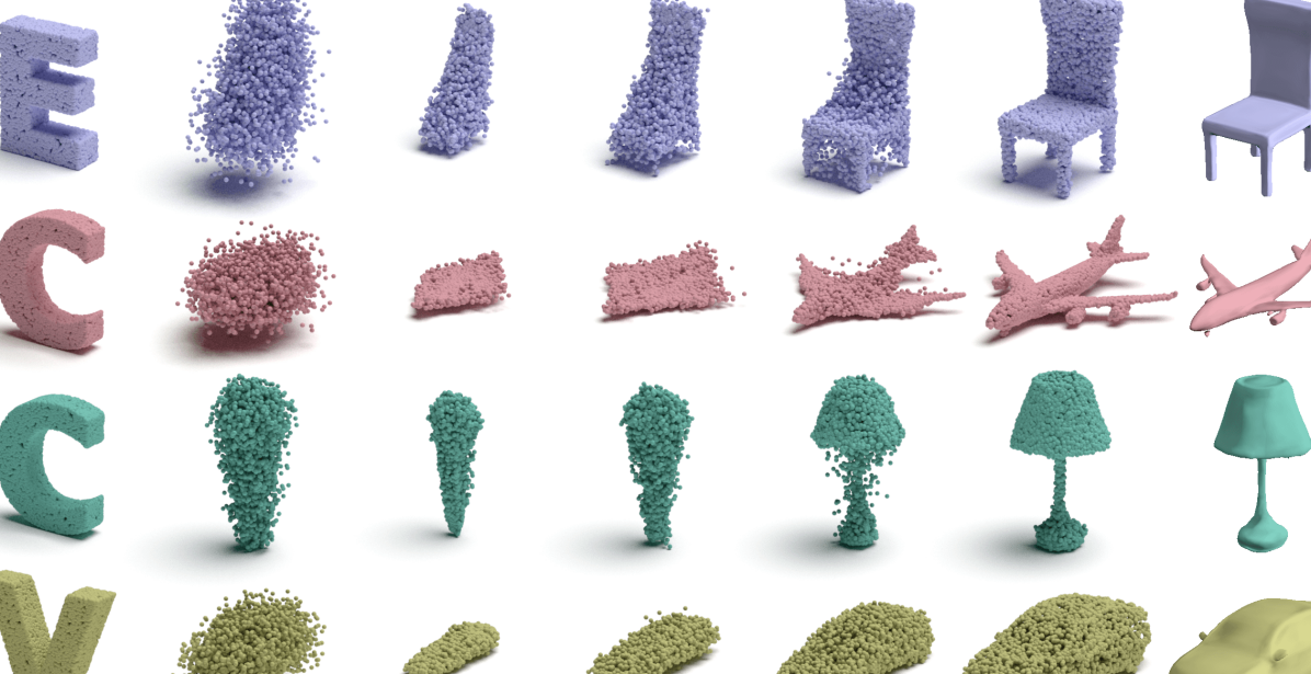
Figure 1: To generate shapes, we sample points from an arbitrary prior (depicting the letters “E”, “C”, “C”, “V” in the examples above) and move them stochastically along a learned gradient field, ultimately reaching the shape’s surface. Our learned fields also enable extracting the surface of the shape, as demonstrated on the right.

1 Introduction

Point clouds are becoming increasingly popular for modeling shapes, as many modern 3D scanning devices process and output point clouds. As such, an increasing number of applications rely on the recognition, manipulation, and synthesis of point clouds. For example, an autonomous vehicle might need to detect cars in sparse LiDAR point clouds. An augmented reality application might need to scan in the environment. Artists may want to further manipulate scanned objects to create new objects and designs. A prior for point clouds would be useful for these applications as it can densify LiDAR clouds, create additional training data for recognition, complete scanned objects or synthesize new ones. Such a prior requires a powerful generative model for point clouds.

In this work, we are interested in learning a generative model that can sample shapes represented as point clouds. A key challenge here is that point clouds are sets of arbitrary size. Prior work often generates a fixed number of points instead [2, 18, 68, 52, 17]. This number, however, may be insufficient for some applications and shapes, or too computationally expensive for others. Instead, following recent works [33, 64, 56], we consider a point cloud as a set of samples from an underlying distribution of 3D points. This new perspective not only allows one to generate an arbitrary number of points from a shape, but also makes it possible to model shapes with varying topologies. However, it is not clear how to best parameterize such a distribution of points, and how to learn it using only a limited number of sampled points.

Prior research has explored modeling the distribution of points that represent the shape using generative adversarial networks (GANs) [33], flow-based models [64], and autoregressive models [56]. While substantial progress has been made, these methods have some inherent limitations for modeling the distribution representing a 3D shape. The training procedure can be unstable for GANs or prohibitively slow for invertible models, while autoregressive models assume an ordering, restricting their flexibility for point cloud generation. Implicit representations such as DeepSDF [47] and OccupancyNet [39] can be viewed as modeling this probability density of the 3D points directly, but these models require ground truth signed distance fields or occupancy fields, which are difficult to obtain from point cloud data alone without corresponding meshes.

In this paper, we take a different approach and focus on the end goal – being able to draw an arbitrary number of samples from the distribution of points. Working backward from this goal, we observe that the sampling procedure can be viewed as moving points from a generic prior distribution towards high likelihood regions of the shape (i.e., the surface of the shape). One way to achieve that is to move points gradually, following the gradient direction, which indicates where the density grows the most [61]. To perform such sampling, one only needs to model the gradient of log-density (known as the Stein score function [36]). In this paper, we propose to model a shape by learning the gradient field of its log-density. To learn such a gradient field from a set of sampled points from the shape, we build upon a denoising score matching framework [29, 54]. Once we learn a model that outputs the gradient field, the sampling procedure can be done using a variant of stochastic gradient ascent (i.e. Langevin dynamics [61, 54]).

Our method offers several advantages. First, our model is trained using a simple $L_{2}$ loss between the predicted and a “ground-truth” gradient field estimated from the input point cloud. This objective is much simpler to optimize than adversarial losses used in GAN-based techniques. Second, because it models the gradient directly and does not need to produce a normalized distribution, it imposes minimal restrictions on the model architecture in comparison to flow-based or autoregressive models. This allows us to leverage more expressive networks to model complicated distributions. Because the partition function need not be estimated, our model is also much faster to train. Finally, our model is able to furnish an implicit surface of the shape, as shown in Figure 1, without requiring ground truth surfaces during training. We demonstrate that our technique can achieve state-of-the-art performance in both point cloud auto-encoding and generation. Moreover, our method can retain the same performance when trained with much sparser point clouds.

Our key contributions can be summarized as follows:

• We propose a novel point cloud generation method by extending score-based generative models to learn conditional distributions.

• We propose a novel algorithm to extract high-quality implicit surfaces from the learned model without the supervision from ground truth meshes.

• We show that our model can achieve state-of-the-art performance for point cloud auto-encoding and generation.

2 Related work

Point cloud generative modeling.

Point clouds are widely used for representing and generating 3D shapes due to their simplicity and direct relation to common data acquisition techniques (LiDARs, depth cameras, etc.). Earlier generative models either treat point clouds as a fixed-dimensional matrix (i.e. $N\times 3$ where $N$ is predefined) [2, 18, 67, 56, 68, 17, 52, 59], or relies on heuristic set distance functions such as Chamfer distance and Earth Mover Distance [25, 65, 19, 12, 6]. As pointed out in Yang et al. [64] and Section 1, both of these approaches lead to several drawbacks. Alternatively, we can model the point cloud as samples from a distribution of 3D points. Toward this end, Sun et al. [56] applies an autoregressive model to model the distribution of points, but it requires assuming an ordering while generating points. Li et al. [33] applies a GAN [4, 26] on both this distribution of 3D points as well as the distribution of shapes. PointFlow [64] applies normalizing flow [46] to model such distribution, so sampling points amounts to moving them to the surface according to a learned vector field. In addition to modeling the movement of points, PointFlow also tracks the change of volume in order to normalize the learned distribution, which is computationally expensive [9]. While our work applies a GAN to learn the distribution of latent code similar to Li et al. and Achilioptas et al., we take a different approach to model the distribution of 3D points. Specifically, we predict the gradient of log-density field to model the non-normalized probability density, thus circumventing the need to compute the partition function and achieves faster training time with a simple L2 loss.

Generating other 3D representations.

Common representations emerged for deep generative 3D modeling include voxel-based [23, 63], mesh-based [3, 48, 20, 27, 35, 57], and assembly-based techniques [34, 41]. Recently, implicit representations are gaining increasing popularity, as they are capable of representing shapes with high level of detail [47, 39, 11, 40]. They also allow for learning a structured decomposition of shapes, representing local regions with Gaussian functions [21, 22] or other primitives [58, 53, 28]. In order to reconstruct the mesh surface from the learned implicit field, these methods require finding the zero iso-surface of the learned occupancy field (e.g. using the Marching Cubes algorithm [37]). Our learned gradient field also allows for high-quality surface reconstruction using similar methods. However, we do not require prior information on the shape (e.g., signed distance values) for training, which typically requires a watertight input mesh. Recently, SAL [5] learns a signed distance field using only point cloud as supervision. Different from SAL, our model directly outputs the gradients of the log-density instead field of the signed distance, which allows our model to use arbitrary network architecture without any constraints. As a result, our method can scale to more difficult settings such as train on larger dataset (e.g. ShapeNet [7]) or train with sparse scanned point clouds.

Energy-based modeling.

In contrast to flow-based models [50, 13, 30, 9, 24, 64] and auto-regressive models [56, 43, 45, 44], energy-based models learn a non-normalized probability distribution [31], thus avoid computation to estimate the partition function. It has been successfully applied to tasks such as image segmentation [16, 15], where a normalized probability density function is hard to define. Score matching was first proposed for modeling energy-based models in [29] and deals with “matching” the model and the observed data log-density gradients, by minimizing the squared distance between them. To improve its performance and scalability, various extensions have been proposed, including denoising score matching [60] and sliced score matching [55]. Most recently, Song and Ermon [54] introduced data perturbation and annealed Langevin dynamics to the original denoising score matching method, providing an effective way to model data embedded on a low dimensional manifold. Their method was applied to the image generation task, achieving performance comparable to GANs. In this work, we extend this method to model conditional distributions and demonstrate its suitability to the task of point cloud generation, viewing point clouds as samples from the 2D manifold (shape surface) in 3D space.

3 Method

In this work, we are interested in learning a generative model that can sample shapes represented as point clouds. Therefore, we need to model two distributions. First, we need to model the distribution of shapes, which encode how shapes vary across an entire collection of shapes. Once we can sample a particular shape of interest, then we need a mechanism to sample a point clouds from its surface. As previously discussed, a point cloud is best viewed as samples from a distribution of 3D (or 2D) points, which encode a particular shape. To sample point clouds of arbitrary size for this shape, we also need to model this distribution of points.

Specifically, we assume a set of shapes $\mathcal{X}=\{X^{(i)}\}^{N}_{i=1}$ are provided as input. Each shape in $\mathcal{X}$ is represented as a point cloud sampled from its surface, defined by $X^{(i)}=\{x_{j}^{i}\}_{j=1}^{M_{i}}$. Our goal is to learn both the distribution of shapes and the distribution of points, conditioned on a particular shape from the data. To achieve that, we first propose a model to learn the distribution of points encoding a shape from a set of points $X^{(i)}$ (Section 3.1 - 3.5). Then we describe how to model the distribution of shapes from the set of point clouds (i.e. $\mathcal{X}$) in Section 3.6.

3.1 Shapes as a distribution of 3D points

We would like to define a distribution of 3D points $P(x)$ such that sampling from this distribution will provide us with a surface point cloud of the object. Thus, the probability density encoding the shape should concentrate on the shape surface. Let $S$ be the set of points on the surface and $P_{S}(x)$ be the uniform distribution over the surface. Sampling from $P_{S}(x)$ will create a point cloud uniformly sampled from the surface of interest. However, this distribution is hard to work with: for all points that are not in the surface $x\notin S$, $P_{S}(x)=0$. As a result, $P_{S}(x)$ is discontinuous and has usually zero support over its ambient space (i.e. $\mathbb{R}^{3}$), which impose challenges in learning and modeling. Instead, we approximate $P_{S}(x)$ by smoothing the distribution with a Gaussian kernel:

$$Q_{\sigma,S}(x)=\int_{s\in\mathbb{R}^{3}}P_{S}(s)\mathcal{N}(x;s,\sigma^{2}I)ds.$$ (1)

As long as the standard deviation $\sigma$ is small enough, $Q_{\sigma,S}(x)$ will approximate the true data distribution $P_{S}(x)$ whose density concentrates near the surface. Therefore, sampling from $Q_{\sigma,S}(x)$ will yield points near the surface $S$.

As discussed in Section 1, instead of modeling $Q_{\sigma,S}$ directly, we will model the gradient of the logarithmic density (i.e. $\nabla_{x}\log{Q_{\sigma,S}(x)}$). Sampling can then be performed by starting from a prior distribution and performing gradient ascent on this field, thus moving points to high probability regions.

In particular, we will model the gradient of the log-density using a neural network $g_{\theta}(x,\sigma)$, where $x$ is a location in 3D (or 2D) space. We will first analyze several properties of this gradient field $\nabla_{x}\log{Q_{\sigma,S}(x)}$. Then we describe how we train this neural network and how we sample points using the trained network.

3.2 Analyzing the gradient field

In this section we provide an interpretation of how $\nabla_{x}\log{Q_{\sigma,S}(x)}$ behaves with different $\sigma$’s. Computing a Monte Carlo approximation of $Q_{\sigma,S}(x)$ using a set of observations $\{x_{i}\}_{i=1}^{m}$, we obtain a mixture of Gaussians with modes centered at $x_{i}$ and radially-symmetric kernels:

$$Q_{\sigma,S}(x) =\mathbb{E}_{s\sim P_{S}}\left[\mathcal{N}(x;s,\sigma^{2}I)\right]\approx\frac{1}{m}\sum_{i=1}^{m}\mathcal{N}(x;x_{i},\sigma^{2}I)\triangleq A_{\sigma}(x,\{x_{i}\}_{i=1}^{m}).$$

The gradient field can thus be approximated by the gradient of the logarithmic of this Gaussian mixture:

$$\nabla_{x}\log{A_{\sigma}(x,\{x_{i}\}_{i=1}^{m})}=\frac{1}{\sigma^{2}}\left(-x+\sum_{i=1}^{m}x_{i}w_{i}(x,\sigma)\right),$$ (2)

where the weight $w_{ij}(x,\sigma)$ is computed from a softmax with temperature $2\sigma^{2}$:

$$w_{i}(x,\sigma)=\frac{\exp{\left(-\frac{1}{2\sigma^{2}}\|x-x_{i}\|^{2}\right)}}{\sum_{j=1}^{m}\exp{\left(-\frac{1}{2\sigma^{2}}\|x-x_{j}\|^{2}\right)}}.$$ (3)

Since $\sum_{i}w_{i}(x,\sigma)=1$, $\sum_{i}x_{i}w_{i}(x,\sigma)$ falls within the convex hull created by the sampled surface points $\{x_{i}\}_{i=1}^{m}$. Therefore, the direction of this gradient of the logarithmic density field points from the sampled location towards a point inside the convex hull of the shape. When the temperature is high (i.e. $\sigma$ is large), then the weights $w_{i}(x,\sigma)$ will be roughly the same and $\sum_{i}x_{i}w_{i}(x,\sigma)$ behaves like averaging all the $x_{i}$’s. Therefore, the gradient field will point to a coarse shape that resembles an average of the surface points. When the temperature is low (i.e. $\sigma$ is small), then $w_{i}(x,\sigma)$ will be close to $0$ except when $x_{i}$ is the closest to $x$. As a result, $\sum_{i}x_{i}w_{i}(x,\sigma)$ will behave like an $\operatorname{argmin}_{x_{i}}\|x_{i}-x\|$. The gradient direction will thus point to the nearest point on the surface. In this case, the norm of the gradient field approximates a distance field of the surface up to a constant $\sigma^{-2}$. This allows the gradient field to encode fine details of the shape and move points to the shape surface more precisely. Figure 2 shows a visualization of the field in the 2D case for a series of different $\sigma$’s.

3.3 Training objective

As mentioned in Section 3.1, we would like to train a deep neural network $g_{\theta}(x,\sigma)$ to model the gradient of log-density: $\nabla_{x}\log{Q_{\sigma,S}(x)}$. One simple objective achieving this is minimizing the L2 loss between them [29]:

$$\ell_{\mathsf{direct}}(\sigma,S)=\mathbb{E}_{x\sim Q_{\sigma,S}(x)}\left[\frac{1}{2}\left\|g_{\theta}(x,\sigma)-\nabla_{x}\log{Q_{\sigma,S}(x)}\right\|_{2}^{2}\right].$$ (4)

However, optimizing such an objective is difficult as it is generally hard to compute $\nabla_{x}\log Q_{\sigma,S}(x)$ from a finite set of observations.

Inspired by denoising score matching methods [60, 54], we can write $Q_{\sigma,S}(x)$ as a perturbation of the data distribution $P_{S}(x)$, produced with a Gaussian noise with standard deviation $\sigma$. Specifically, $Q_{\sigma,S}(x)=\int P_{S}(s)q_{\sigma}(\tilde{x}|s)dx$, where $q_{\sigma}(\tilde{x}|s)=\mathcal{N}(\tilde{x}|s,\sigma^{2}I)$. As such, optimizing the objective in Equation 4 can be shown to be equivalent to optimizing the following [60]:

$$\ell_{\mathsf{denoising}}(\sigma,S)=\mathbb{E}_{s\sim P_{S},\tilde{x}\sim q_{\sigma}(\tilde{x}|s)}\left[\frac{1}{2}\|g_{\theta}(\tilde{x},\sigma)-\nabla_{\tilde{x}}\log{q_{\sigma}(\tilde{x}|s)}\|_{2}^{2}\right].$$ (5)

Since $\nabla_{\tilde{x}}\log{q_{\sigma}(\tilde{x}|s)}=\frac{s-\tilde{x}}{\sigma^{2}}$, this loss can be easily computed using the observed point cloud $X=\{x_{j}\}_{j=1}^{m}$ as following:

$$\ell(\sigma,X)=\frac{1}{|X|}\sum_{x_{i}\in X}\|g_{\theta}(\tilde{x_{i}},\sigma)-\frac{x_{i}-\tilde{x}_{i}}{\sigma^{2}}\|_{2}^{2},\quad\tilde{x_{i}}\sim\mathcal{N}(x_{i},\sigma^{2}I).$$ (6)

Multiple noise levels. One problem with the abovementioned objective is that most $\tilde{x_{i}}$ will concentrate near the surface if $\sigma$ is small. Thus, points far away from the surface will not be supervised. This can adversely affect the sampling quality, especially when the prior distribution puts points to be far away from the surface. To alleviate this issue, we follow Song and Ermon [54] and train $g_{\theta}$ for multiple $\sigma$’s, with $\sigma_{1}\geq\dots\geq\sigma_{k}$. Our final model is trained by jointly optimizing $\ell(\sigma_{i},X)$ for all $\sigma_{i}$. The final objective is computed empirically as:

$$\mathcal{L}(\{\sigma_{i}\}_{i=1}^{k},X)=\sum_{i=1}^{k}\lambda(\sigma_{i})\ell(\sigma_{i},X),$$ (7)

where $\lambda(\sigma_{i})$ are parameters weighing the losses $\ell(\sigma_{i},X)$. $\lambda(\sigma_{i})$ is chosen so that the weighted losses roughly have the same magnitude during training.

3.4 Point cloud sampling

Sampling a point cloud from the distribution is equivalent to moving points from a prior distribution to the surface (i.e. the high-density region). Therefore, we can perform stochastic gradient ascent on the logarithmic density field. Since $g_{\theta}(x,\sigma)$ approximates the gradient of the log-density field (i.e. $\nabla_{x}\log{Q_{\sigma,S}(x)}$), we could thus use $g_{\theta}(x,\sigma)$ to update the point location $x$. In order for the points to reach all the local maxima, we also need to inject random noise into this process. This amounts to using Langevin dynamics to perform sampling [61].

Specifically, we first sample a point $x_{0}$ from a prior distribution $\pi$. The prior is usually chosen to be simple distribution such as a uniform or a Gaussian distribution. We empirically demonstrate that the sampling performance won’t be affected as long as the prior points are sampled from places where the perturbed points would reach during training. We then perform the following recursive update with step size $\alpha>0$:

$$x_{t+1}=x_{t}+\frac{\alpha}{2}g_{\theta}(x_{t},\sigma)+\sqrt{\alpha}\epsilon_{t},\quad\epsilon_{t}\sim\mathcal{N}(0,I).$$ (8)

Under mild conditions, $p(x_{T})$ converges to the data distribution $Q_{\sigma,S}(x)$ as $T\to\infty$ and $\epsilon\to 0$ [61]. Even when such conditions fail to hold, the error in Equation 8 is usually negligible when $\alpha$ is small and $T$ is large [54, 10, 14, 42].

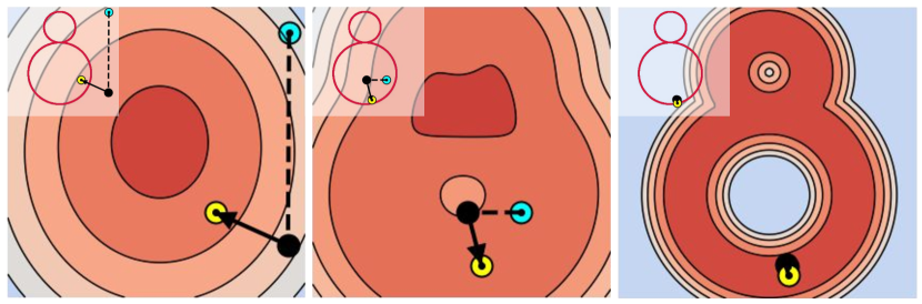
Figure 2: Log density field with different $\sigma$ (biggest to smallest) and a Langevin Dynamic point update step with that $\sigma$. Deeper color indicates higher density. The ground truth shape is shown in the upper left corner. Dotted line indicated Gaussian noise and solid arrows indicates gradient step. As sigma decreases, the log-density field changes from coarse to fine, and points are moved closer to the surface.

Prior works have observed that a main challenge for using Langevin dynamics is its slow mixing time [54, 62]. To alleviate this issue, Song and Ermon [54] propose an annealed version of Langevin dynamics, which gradually anneals the noise for the score function. Specifically, we first define a list of $\sigma_{i}$ with $\sigma_{1}\geq\dots\geq\sigma_{k}$, then train one single denoising score matching model that could approximate $q_{\sigma_{i}}$ for all $i$. Then, annealed Langevin dynamics will recursively compute the $x_{t}$ while gradually decreasing $\sigma_{i}$:

$$x_{t+1}^{\prime} =x_{t}+\frac{\sqrt{\alpha}\sigma_{i}\epsilon_{t}}{\sigma_{k}},\quad\epsilon_{t}\sim\mathcal{N}(0,I),$$ (9)

$$x_{t+1} =x_{t+1}^{\prime}+\frac{\alpha\sigma_{i}^{2}}{2\sigma_{k}^{2}}g_{\theta}(x_{t+1}^{\prime},\sigma_{i}).~{}$$ (10)

Figure 2 demonstrates the sampling across the annealing process in a 2D point cloud. As discussed in Section 3.3, larger $\sigma$’s correspond to coarse shapes while smaller $\sigma$’s correspond to fine shape. Thus, this annealed Langevin dynamics can be thought of as a coarse-to-fine refinement of the shape. Note that we make the noise perturnbation step before the gradient update step, which leads to cleaner point clouds. The supplementary material contains detailed hyperparameters.

3.5 Implicit surface extraction

Next we show that our learned gradient field (e.g. $g_{\theta}$) also allows for obtaining an implicit surface. The key insight here is that the surface is defined as the set of points that reach the maximum density in the data distribution $P_{S}(x)$, and thus these points have zero gradient. Another interpretation is that when $\sigma$ is small enough (i.e. $Q_{\sigma,S}(x)$ approximates the true data distribution $p(x)$), the gradient for points near the surface will point to its nearest point on the surface, as described in Section 3.2:

$$g_{\theta}(x,\sigma)\approx\frac{1}{\sigma^{2}}\left(-x+\operatorname{argmin}_{s\in S}\|x-s\|\right).$$ (11)

Thus, for a point near the surface, its norm equals zero if and only if $x\in S$ (provided the $\arg\min$ is unique). Therefore, the shape can be approximated by the zero iso-surface of the gradient norm:

$$S\approx\{x~{}|~{}\|g_{\theta}(x,\sigma)\|=\delta\},$$ (12)

for some $\delta>0$ that is sufficiently small. One caveat is that points for which the $\arg\min$ in Equation 11 is not unique may also have a zero gradient. These correspond to local minimas of the likelihood. In practice, this is seldom a problem for surface extraction, and it is possible to discard these regions by conducting the second partial derivative test.

Also as mentioned in Section 3.2, when the $\sigma$ is small, the norm of the gradient field approximates a distance field of the surface, scaled by a constant $\sigma^{-2}$. This allows us to retrieval the surface $S$ efficiently using an off-the-shelf ray-casting technique [51] (see Figures 1,4,5).

3.6 Generating multiple shapes

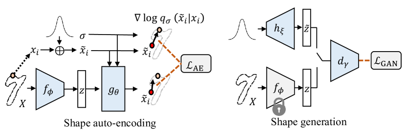
Figure 3: Illustration of training pipe for shape auto-encoding and generation.

In the previous sections, we focused on learning the distribution of points that represent a single shape. Our next goal is to model the distribution of shapes. We, therefore, introduce a latent code $z$ to encode which specific shape we want to sample point clouds from. Furthermore, we adapt our gradient decoder to be conditional on the latent code $z$ (in addition to $\sigma$ and the sampled point).

As illustrated in Figure 3, the training is conducted in two stages. We first train an auto-encoder with an encoder $f_{\phi}$ that takes a point cloud and outputs the latent code $z$. The gradient decoder is provided with $z$ as input and produces a gradient field with noise level $\sigma$. The auto-encoding loss is thus:

$$\mathcal{L}_{AE}(\mathcal{X})=\mathop{\mathbb{E}}_{X\sim\mathcal{X}}\left[\frac{1}{2|X|}\sum_{x\in X,\sigma_{i}}\lambda(\sigma_{i})\left\|g_{\theta}(\tilde{x},f_{\phi}(X),\sigma_{i})-\frac{x-\tilde{x}}{\sigma_{i}^{2}}\right\|_{2}^{2}\right],$$ (13)

where each $\tilde{x_{j}}$ is drawn from a $\mathcal{N}(x_{j},\sigma_{i}^{2}I)$ for a corresponding $\sigma_{i}$. This first stage provides us with a network that can model the distribution of points representing the shape encoded in the latent variable $z$. Once the auto-encoder is fully trained, we apply a latent-GAN [2] to learn the distribution of the latent code $p(z)=p(f_{\phi}(X))$, where $X$ is a point cloud sampled from the data distribution. Doing so provides us with a generator $h_{\xi}$ that can sample a latent code from $p(z)$, allowing us control over which shape will be generated. To sample a novel shape, we first sample a latent code $\tilde{z}$ using $h_{\xi}$. We can then use the trained gradient decoder $g_{\theta}$ to sample point clouds or extract an implicit surface from the shape represented as $z$. For more details about hyperparameters and model architecture, please refer to the supplementary material.

4 Experiments

In this section, we will evaluate our model’s performance in point cloud auto-encoding (Sec 4.1), up-sampling (Sec 4.1), and generation (Sec 4.2) tasks. Finally, we present an ablation study examining our model design choices (Sec 4.3). Implementation details will be shown in the supplementary materials.

4.0.1 Datasets

Our experiments focus mainly on two datasets: MNIST-CP and ShapeNet. MNIST-CP was recently proposed by Yifan et al. [66] and consists of 2D contour points extracted from the MNIST [32] dataset, which contains 50K and 10K training and testing images. Each point cloud contains 800 points. The ShapeNet [8] dataset contains 35708 shapes in training set and 5158 shapes in test set, capturing 55 categories. For our method, we normalize all point clouds by centering their bounding boxes to the origin and scaling them by a constant such that all points range within the cube $[-1,1]^{3}$ (or the square in the 2D case).

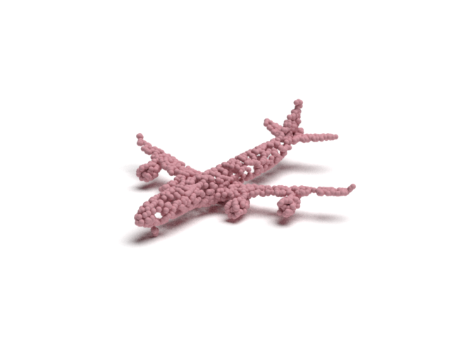
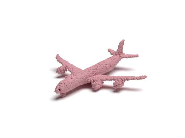
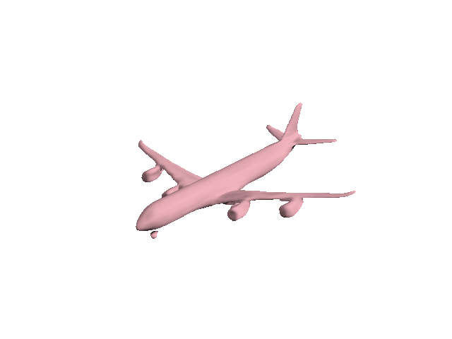
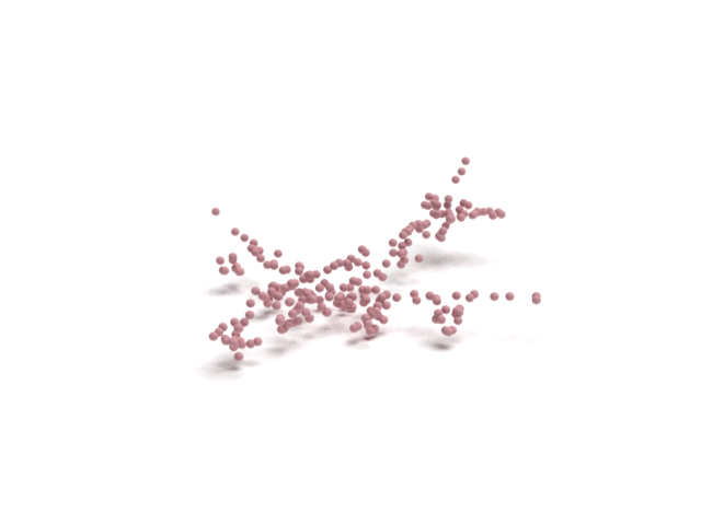
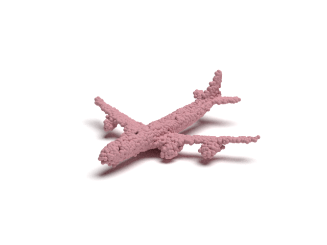
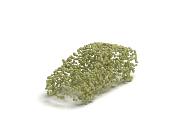
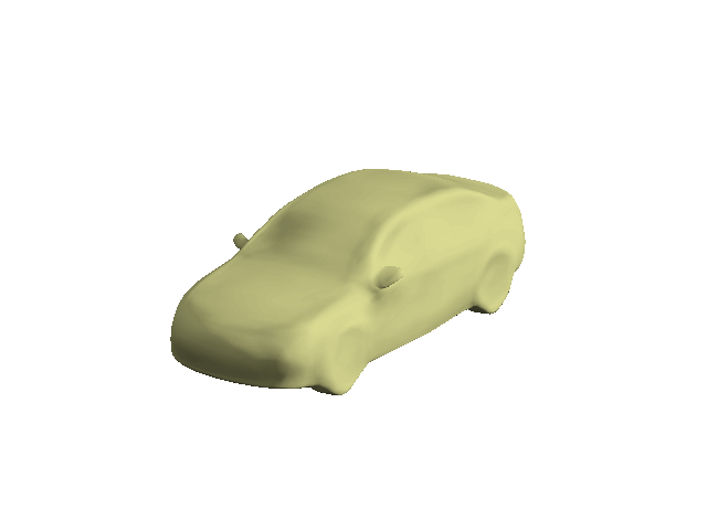
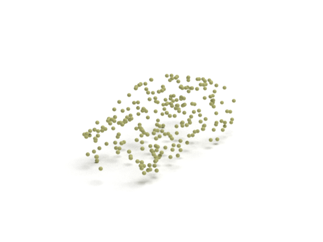
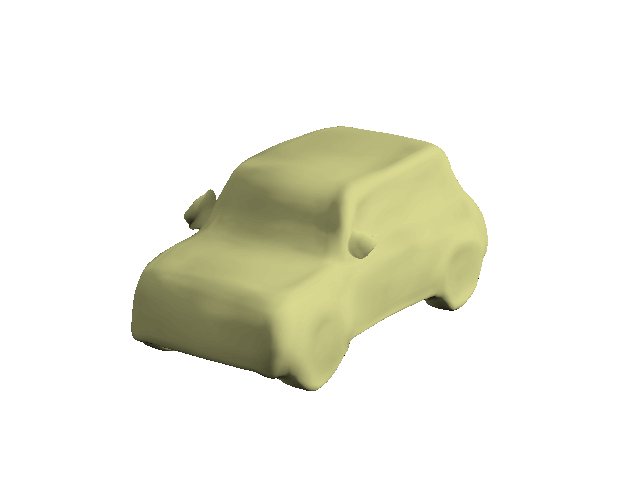
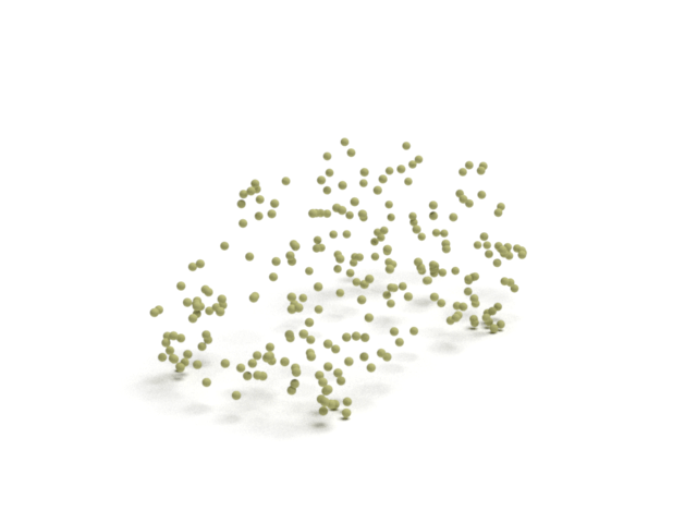
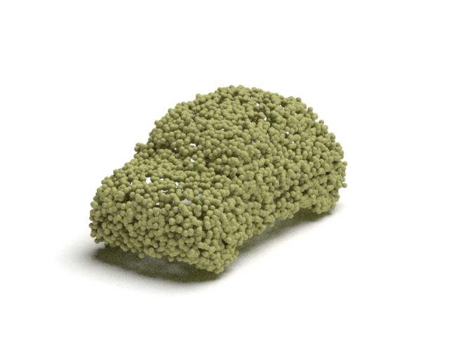
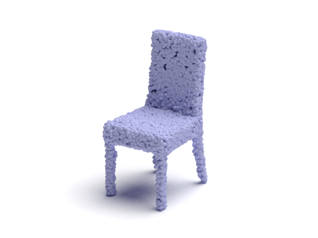
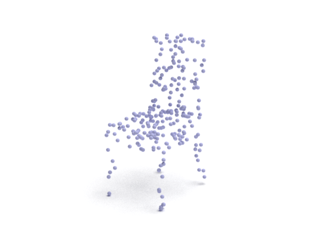
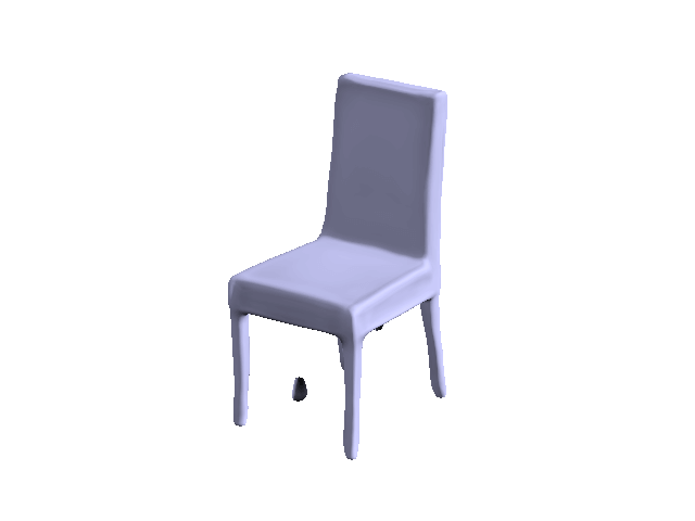
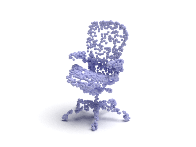
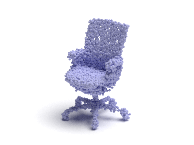
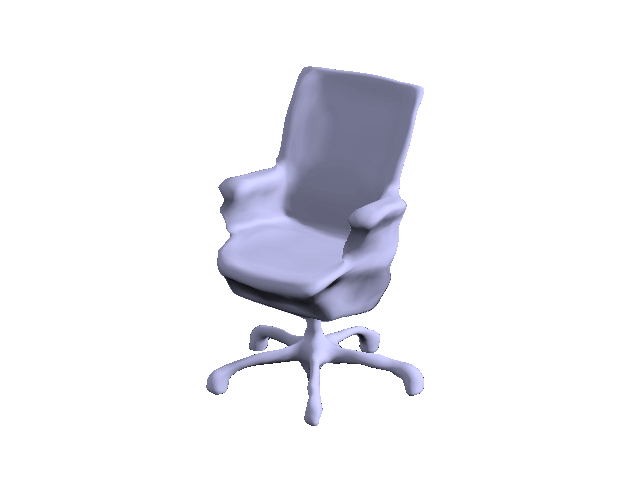
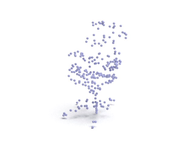
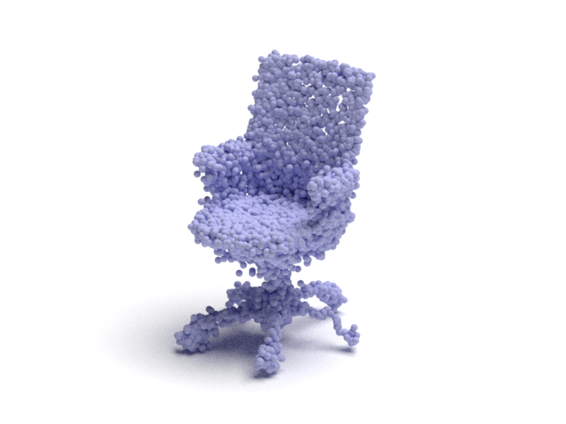
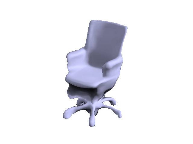
Figure 4: Shape auto-encoding test results. Our model can accurately reconstruct shapes given 2048 points (left) or only 256 points (right) describing the shape. Output point clouds are illustrated in the center and implicit surfaces on the left.

4.0.2 Evaluation metrics

Following prior works [64, 25, 2], we use the symmetric Chamfer Distance (CD) and the Earth Mover’s Distance (EMD) to evaluate the reconstruction quality of the point clouds. To evaluate the generation quality, we use metrics in Yang et al. [64] and Achlioptas et al. [2]. Specifically, Achilioptas et al. [2] suggest using Minimum Matching Distance (MMD) to measure fidelity of the generated point cloud and Coverage (COV) to measure whether the set of generated samples cover all the modes of the data distribution. Yang et al. [64] propose to use the accuracy of a $k$-NN classifier performing two-sample tests. The idea is that if the sampled shapes seem to be drawn from the actual data distribution, then the classifier will perform like a random guess (i.e. results in $50\%$ accuracy). To evaluate our results, we first conduct per-shape normalization to center the bounding box of the shape and scale its longest length to be 2, which allows the metric to focus on the geometry of the shape and not the scale.

4.1 Shape auto-encoding

Table 1: Shape auto-encoding on the MNIST-CP and ShapeNet datasets. The best results are highlighted in bold. CD is multiplied by $10^{4}$ and EMD is multiplied by $10^{2}$.

		l-GAN [2]		AtlasNet [25]		PF [64]	Ours	Oracle
Dataset	Metric	CD	EMD	Sphere	Patches
MNIST-CP	CD	8.204	-	7.274	4.926	17.894	2.669	1.012
	EMD	40.610	-	19.920	15.970	8.705	7.341	4.875
Airplane	CD	1.020	1.196	1.002	0.969	1.208	0.96	0.837
	EMD	4.089	2.577	2.672	2.612	2.757	2.562	2.062
Chair	CD	9.279	11.21	6.564	6.693	10.120	5.599	3.201
	EMD	8.235	6.053	5.790	5.509	6.434	4.917	3.297
Car	CD	5.802	6.486	5.392	5.441	6.531	5.328	3.904
	EMD	5.790	4.780	4.587	4.570	5.138	4.409	3.251
ShapeNet	CD	7.120	8.850	5.301	5.121	7.551	5.154	3.031
	EMD	7.950	5.260	5.553	5.493	5.176	4.603	3.103

In this section, we evaluate how well our model can learn the underlying distribution of points by asking it to auto-encode a point cloud. We conduct the auto-encoding task for five settings: all 2D point clouds in MNIST-CP, 3D point clouds on the whole ShapeNet, and three categories in ShapeNet (Airplane, Car, Chair). In this experiment, our method is compared with the current state-of-the-art AtlasNet [25] with patches and with sphere. Furthermore, we also compare against Achilioptas et al. [2] which predicts point clouds as a fixed-dimensional array, and PointFlow [64] which uses a flow-based model to represent the distribution. We follow the experiment set-up in PointFlow to report performance in both CD and EMD in Table 1. Since these two metrics depend on the scale of the point clouds, we also report the upper bound in the “oracle” column. The upper bound is produced by computing the error between two different point clouds with the same number of points sampled from the same underlying meshes.

Our method consistently outperforms all other methods on the EMD metric, which suggests that our point samples follow the distribution or they are more uniformly distributed among the surface. Note that our method outperforms PointFlow in both CD and EMD for all datasets, but requires much less time to train. Our training for the Airplane category can be completed in about less than 10 hours, yet reproducing the results for PointFlow’s pretrained model takes at least two days. Our method can even sometimes outperform Achilioptas et al.and AtlasNet in CD, which is the loss they are directly optimizing at.

Table 2: Auto-encoding sparse point clouds. We randomly sample $N$ points from each shape (in the Airplane dataset). During training, the model is provided with $M$ points (the columns). CD is multiplied by $10^{4}$ and EMD is multiplied by $10^{2}$.

	CD						EMD
N	2048	1024	512	256	128		2048	1024	512	256	128
$10K$	0.993	1.057	0.999	1.136	1.688		2.463	2.608	2.589	3.042	3.715
$3K$	1.080	1.059	1.003	1.142	1.753		2.533	2.586	2.557	2.997	3.878
$1K$	-	-	1.021	1.149	1.691		-	-	2.565	2.943	3.633

Point cloud upsampling

We conduct a set of experiments on subsampled ShapeNet point clouds. These experiments are primarily focused on showing that (i) our model can learn from sparser datasets, and that (ii) we can infer a dense shape from a sparse input. In the regular configuration (reported above), we learn from $N=10K$ points which are uniformly sampled from each shape mesh model. During training, we sample $M=2048$ points (from the $10K$ available in total) to be the input point cloud. To evaluate our model, we perform the Langevin dynamic procedure (described in Section 3.4) over $2048$ points sampled from the prior distribution and compare these to $2048$ points from the reference set.

To evaluate whether our model can effectively upsample point clouds and learn from a sparse input, we train models with $N=[1K,3K,10K]$ and $M=[128,256,512,1024,2048]$ on the Airplane dataset. To allow for a fair comparison, we evaluate all models using the same number of output points (i.e. $2048$ points are sampled from the prior distribution in all cases). As illustrated in Table 2, we obtain comparable auto-encoding performance while training with significantly sparser shapes. Interestingly, the number of points available from the model (i.e. $N$) does not seem to affect performance, suggesting that we can indeed learn from sparser datasets. Several qualitative examples auto-encoding shapes from the regular and sparse configurations are shown in Figure 4. We also demonstrate that our model can also provide a smooth iso-surface, even when only a sparse point cloud (i.e. 256 points) is provided as input.

4.2 Shape generation

We quantitatively compare our method’s performance on shape generation with r-GAN [2], GCN-GAN [59], TreeGAN [52], and PointFlow [64]. We use the same experiment setup as PointFlow except for the data normalization before the evaluation. The generation results are reported in Table 3. Though our model requires a two-stage training, the training can be done within one day with a 1080 Ti GPU, while reproducing PointFlow’s results requires training for at least two days on the same hardware. Despite using much less training time, our model achieves comparable performance to PointFlow, the current state-of-the-art. As demonstrated in Figure 5, our generated shapes are also visually cleaner.

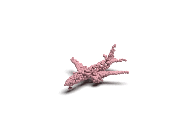
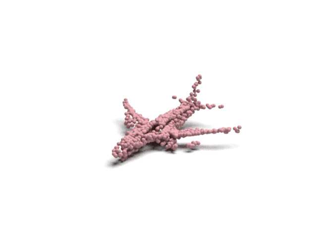
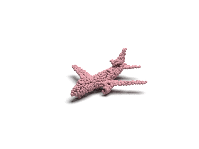
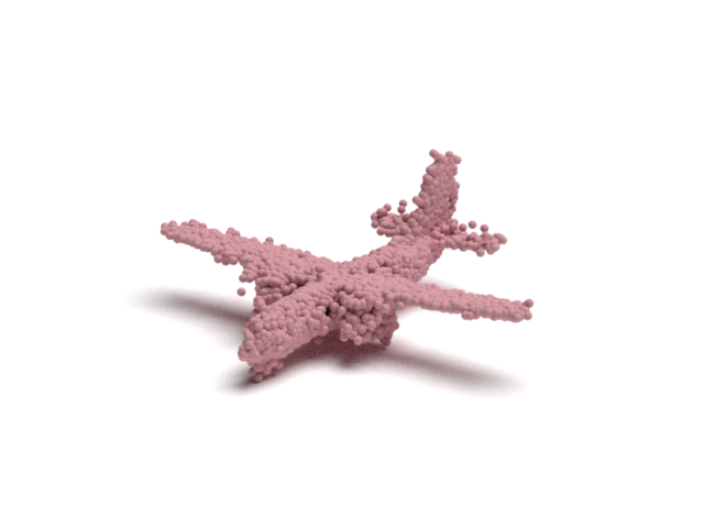
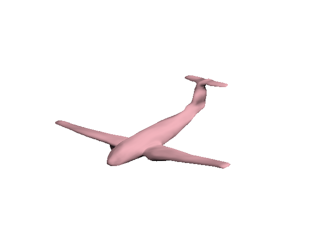
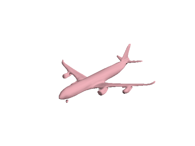
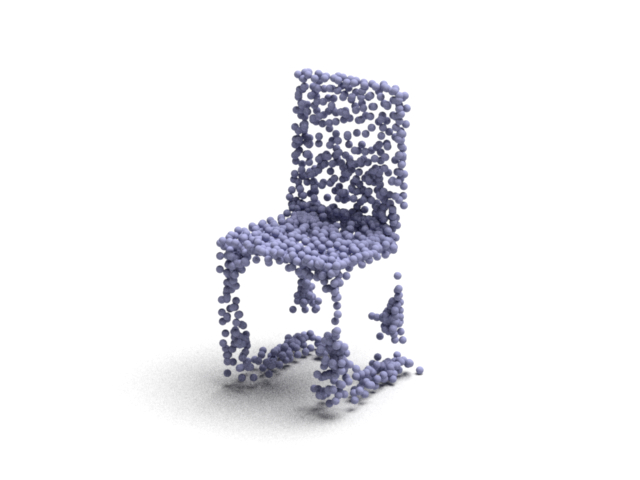
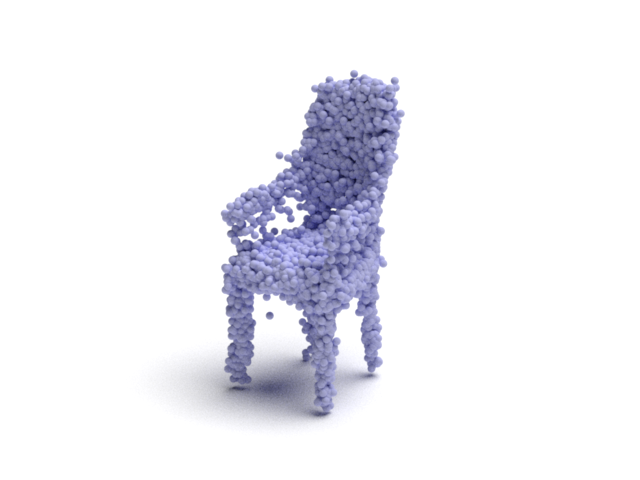
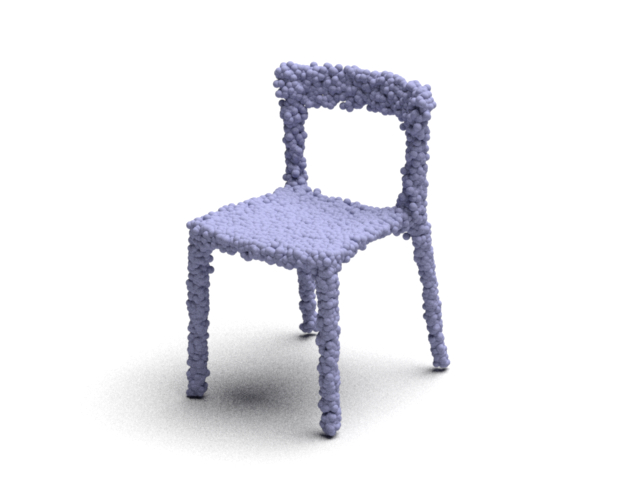
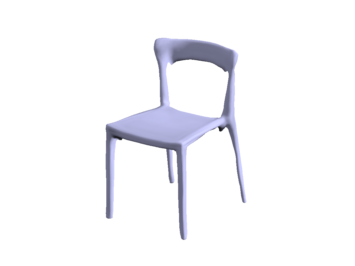
r-GAN	CGN	Tree	PF	Ours

Figure 5: Generation results. We shown results from r-GAN, GCN, TreeGAN (Tree), and PointFlow (PF) are illustrated on the left for comparison. Generated point clouds are illustrated alongside the corresponding implicit surfaces.

Table 3: Shape generation results. $\uparrow$ means the higher the better, $\downarrow$ means the lower the better. MMD-CD is multiplied by $10^{3}$ and MMD-EMD is multiplied by $10^{2}$.

		MMD ($\downarrow$)			COV (%, $\uparrow$)			1-NNA (%, $\downarrow$)
Category	Model	CD	EMD		CD	EMD		CD	EMD
Airplane	r-GAN [2]	1.657	13.287		38.52	19.75		95.80	100.00
	GCN [59]	2.623	15.535		9.38	5.93		95.16	99.12
	Tree [52]	1.466	16.662		44.69	6.91		95.06	100.00
	PF [64]	1.408	7.576		39.51	41.98		83.21	82.22
	Ours	1.285	7.364		47.65	41.98		85.06	83.46
	Train	1.288	7.036		45.43	45.43		72.10	69.38
Chair	r-GAN [2]	18.187	32.688		19.49	8.31		84.82	99.92
	GCN [59]	23.098	25.781		6.95	6.34		86.52	96.48
	Tree [52]	16.147	36.545		40.33	8.76		74.55	99.92
	PF [64]	15.027	19.190		40.94	44.41		67.60	72.28
	Ours	14.818	18.791		46.37	46.22		66.16	59.82
	Train	15.893	18.472		50.45	52.11		53.93	54.15

Table 4: Ablation study comparing auto-encoding performance on the Airplane dataset. CD is multiplied by $10^{4}$ and EMD is multiplied by $10^{2}$.

	Single noise level			Prior distribution
Metric	0.1	0.05	0.01	Uniform	Fixed	Gaussian
CD	2.545	1.573	1009.357	0.993	0.993	0.996
EMD	4.400	8.455	36.715	2.463	2.476	2.475

4.3 Ablation study

We conduct an ablation study quantifying the importance of learning with multiple noise levels. As detailed in Sections 3.3-3.4, we train $s_{\theta}$ for multiple $\sigma$’s. During inference, we sample point clouds using an annealed Langevin dynamics procedure, using the same $\sigma$’s seen during training. In Table 4 we show results for models trained with a single noise level and tested without annealing. As illustrated in the table, the model does not perform as well when learning using a single noise level only. This is especially noticeable for the model trained on the smallest noise level in our model ($\sigma=0.01$), as large regions in space are left unsupervised, resulting in significant errors.

We also demonstrate that our model is insensitive to the choice of the prior distribution. We repeat the inference procedure for our auto-encoding experiment, initializing the prior points with a Gaussian distribution or in a fixed location (using the same trained model). Results are reported on the right side of Table 4. Different prior configurations don’t affect the performance, which is expected due to the stochastic nature of our solution. We further demonstrate our model’s robustness to the prior distribution in Figure 1, where the prior depicts 3D letters.

5 Conclusions

In this work, we propose a generative model for point clouds which learns the gradient field of the logarithmic density function encoding a shape. Our method not only allows sampling of high-quality point clouds, but also enables extraction of the underlying surface of the shape. We demonstrate the effectiveness of our model on point cloud auto-encoding, generation, and super-resolution. Future work includes extending our work to model texture, appearance, and scenes.

Acknowledgment. This work was supported in part by grants from Magic Leap and Facebook AI, and the Zuckerman STEM leadership program.

Appendix 0.A Overview

In this appendix, we provide additional method details, implementation details, experimental results, and qualitative results visualizations.

1. Section 0.B Method Details - Additional details about the method including algorithm blocks of training, inference and surface extraction, and the proof of equivalent objective function.

2. Section 0.C Implementation Details - Description of the network architecture, experimental setting, and implementation details.

3. Section 0.D Additional Quantitative Results - More quantitative results on shape generation and implicit surface tasks, comparing our model with additional baselines.

4. Section 0.E Additional Ablation Studies - Results of additional ablation studies.

5. Section 0.F Additional Qualitative Results - Additional qualitative results on scanned data, visualization of latent space, and extended visualizations for 2D and 3D point clouds.

Appendix 0.B Method Details

In this section, we provide extensive details of our method. We provide detailed explanations for training and inference in Section 0.B.1. More details about surface extraction are provided in Section 0.B.2. Finally, a mathematical proof about our objective function is shown in Section 0.B.3.

0.B.1 Training and inference

We provide algorithm blocks to better illustrate the training and inference procedures. See Algorithm 1 and Algorithm 2 for training and inference, respectively. Please refer to Section 0.C for hyper-parameters and neural network architectures.

Algorithm 1 Training.

0:  Noise levels $\{\sigma_{i}\}_{i=1}^{k}$; Weight for noise levels’ loss $\lambda(\sigma_{i})$; Point cloud encoder $f_{\phi}$; A neural network $s_{\theta}$; Total number of training iterations $T$; Point cloud $X_{t}$

1:  for $t\leftarrow 1$ to $T$ do

2:     $z\leftarrow f_{\phi}(X_{t})$

3:     for $\sigma\in\{\sigma_{i}\}_{i=1}^{k}$ do

4:        for $x_{i}\in X_{t}$ do

5:           $\tilde{x}_{i}\leftarrow x_{i}+N(0,\sigma^{2}I)$

6:        end for

7:        $\ell(\sigma,X_{t})\leftarrow\frac{1}{|X_{t}|}\sum_{x_{i}\in X_{t}}\|g_{\theta}(\tilde{x_{i}},\sigma,z)-\frac{x_{i}-\tilde{x}_{i}}{\sigma^{2}}\|_{2}^{2}$

8:     end for

9:     $\mathcal{L}(\{\sigma_{i}\}_{i=1}^{k},X_{t})\leftarrow\sum_{i=1}^{k}\lambda(\sigma_{i})\ell(\sigma_{i},X_{t})$

10:     $\phi,\theta\leftarrow Adam(\mathcal{L},\phi,\theta)$

11:  end for

12:  return  $f_{\phi}$, $s_{\theta}$

Algorithm 2 Annealed Langevin dynamics.

0:  Noise levels $\{\sigma_{i}\}_{i=1}^{k}$; Step size $\alpha$; Number of steps $T$

1:  Initialize $x_{0}$ 

2:  for $i\leftarrow 1$ to $k$ do

3:     for $t\leftarrow 0$ to $T-1$ do

4:        $\epsilon_{t}\sim\mathcal{N}(0,I)$

5:        $x_{t+1}^{\prime}\leftarrow x_{t}+\frac{\sqrt{\alpha}\sigma_{i}\epsilon_{t}}{\sigma_{k}}$

6:        $x_{t+1}\leftarrow x_{t+1}^{\prime}+\frac{\alpha\sigma_{i}^{2}}{2\sigma_{k}^{2}}g_{\theta}(x_{t+1}^{\prime},\sigma_{i})$

7:     end for

8:     $x_{0}\leftarrow x_{T}$

9:  end for

10:  return  $x_{T}$

0.B.2 Surface extraction

We use a modified version of the volumetric ray casting algorithm [51] to render the iso-surface produced by the learned gradient field. Algorithm 3 below shows the rendering process of a single pixel. For each pixel in the rendered image, we cast a ray $\langle o_{0},u\rangle$ towards the gradient field according to the camera model. We advance the ray for a fixed number of steps $k_{\mathrm{max}}$. For reasonable choices of the step rate $\gamma$, the ray will either converge to the iso-surface, or miss the iso-surface and march towards infinity. If the ray does reach the iso-surface, we calculate the RGB values for that pixel based on its 3D location and surface normal. If the ray misses the surface, we assign the pixel with background color $y_{\mathrm{bg}}$. In this paper, we use $\gamma=1.0$, $k_{\mathrm{max}}=64$ and $\delta=0.005$.

Algorithm 3 Ray Casting for Rendering the Iso-surface.

0:  Neural network $s_{\theta}$; Minimum noise level $\sigma_{k}$; Initial ray origin $o_{0}$; Ray direction $u$; Maximum ray travel $d_{\mathrm{max}}$; Step rate $\gamma$; Number of steps $k_{\mathrm{max}}$; Iso-surface level $\delta$; Background color $y_{\mathrm{bg}}$

1:  $d=0$ 

2:  for $k\leftarrow 1$ to $k_{\mathrm{max}}$ do

3:     $x\leftarrow o_{0}+du$

4:     $d\leftarrow d+\gamma(\|s_{\theta}(x,\sigma_{k})\|-\delta)$

5:  end for

6:  if $d<d_{\mathrm{max}}$ then

7:     $n\leftarrow-\frac{s_{\theta}(x,\sigma_{k})}{\|s_{\theta}(x,\sigma_{k})\|}$

8:     $y\leftarrow\mathrm{Shading}(x,n)$

9:  else

10:     $y\leftarrow y_{\mathrm{bg}}$

11:  end if

12:  return  $y$

0.B.3 Objective Function

Here, we provide a proof to show that optimizing $\ell_{\text{direct}}(\sigma,S)$ (Equation 4 in the main paper) is equivalent to optimizing $\ell_{\text{denoising}}(\sigma,S)$ (Equation 5 in the main paper). The proof is largely similar to the one in the Appendix in Vincent 2010 [60]. We will re-visit the prove here using the notation from our paper for convenience of the readers.

Theorem 0.B.1

Optimizing $\ell_{\text{denoise}}(\sigma,S)$ leads to the same $\theta$ as optimizing $\ell_{\text{denoise}}(\sigma,S)$.

Proof

We want to show that $\ell_{\text{direct}}(\sigma,S)=\ell_{\text{denoise}}(\sigma,S)+C$ for some constant $C$ that doesn’t depend on $\theta$. Note that $\ell_{\text{denoise}}$ can be decomposed as follows:

$$\ell_{\text{denoise}}(\sigma,S) =\mathbb{E}_{x\sim P_{S},\tilde{x}\sim q_{\sigma}(\tilde{x}|x)}\left[\frac{1}{2}\|g_{\theta}(\tilde{x},\sigma)\|^{2}\right]$$

$$\quad-\mathbb{E}_{x\sim P_{S},\tilde{x}\sim q_{\sigma}(\tilde{x}|x)}\left[g_{\theta}(\tilde{x},\sigma)^{T}\nabla_{\tilde{x}}\log{q_{\sigma}(\tilde{x}|x)}\right]+C_{1},$$ (14)

where $C_{1}=\mathbb{E}_{x\sim P_{S},\tilde{x}\sim q_{\sigma}(\tilde{x}|s)}\left[\frac{1}{2}\left\|\nabla_{\tilde{x}}\log{q_{\sigma}(\tilde{x}|x)}\right\|^{2}\right]$. Similarly, we can decompose $\ell_{\text{direct}}$ as follows:

$$\ell_{\text{direct}}(\sigma,S) =\mathbb{E}_{x\sim Q_{\sigma,S}}\left[\frac{1}{2}\|g_{\theta}(x,\sigma)\|^{2}\right]$$

$$\quad-\mathbb{E}_{x\sim Q_{\sigma,S}}\left[g_{\theta}(x,\sigma)^{T}\nabla_{x}\log{Q_{\sigma,S}(x)}\right]+C_{2},$$ (15)

where $C_{2}=\mathbb{E}_{x\sim Q_{\sigma,S}}\left[\frac{1}{2}\|\nabla_{x}\log{Q_{\sigma,S}(x)}\|^{2}\right]$. Now we will compare the first two terms of Equation 14 and Equation 15 to show they are the same. Looking at the first terms:

$$\mathbb{E}_{s\sim P_{S},\tilde{x}\sim q_{\sigma}(\tilde{x}|s)}\left[\frac{1}{2}\|g_{\theta}(\tilde{x},\sigma)\|^{2}\right]$$

$$\quad=\frac{1}{2}\int_{x}P_{S}(x)\int_{\tilde{x}}q_{\sigma}(\tilde{x}|x)\|g_{\theta}(\tilde{x},\sigma)\|^{2}d\tilde{x}dx$$

$$\quad=\frac{1}{2}\int_{\tilde{x}}\int_{x}P_{S}(x)q_{\sigma}(\tilde{x}|x)\|g_{\theta}(\tilde{x},\sigma)\|^{2}dxd\tilde{x}$$

$$\quad=\frac{1}{2}\int_{\tilde{x}}\|g_{\theta}(\tilde{x},\sigma)\|^{2}\int_{x}P_{S}(x)q_{\sigma}(\tilde{x}|x)dxd\tilde{x}$$

$$\quad=\frac{1}{2}\int_{\tilde{x}}\|g_{\theta}(\tilde{x},\sigma)\|^{2}Q_{\sigma,S}(\tilde{x})d\tilde{x}\quad\left(\text{since }Q_{\sigma,S}(x)=\int_{y}P_{S}(y)q_{\sigma}(x|y)dy\right)$$

$$\quad=\mathbb{E}_{x\sim Q_{\sigma,S}}\left[\frac{1}{2}\|g_{\theta}(x,\sigma)\|^{2}\right].$$

Looking at the second terms:

$$\mathbb{E}_{x\sim P_{S},\tilde{x}\sim q_{\sigma}(\tilde{x}|x)}\left[g_{\theta}(\tilde{x},\sigma)^{T}\nabla_{\tilde{x}}\log{q_{\sigma}(\tilde{x}|x)}\right]$$

$$\quad=\int_{x}P_{S}(x)\int_{\tilde{x}}q_{\sigma}(\tilde{x}|x)g_{\theta}(\tilde{x},\sigma)^{T}\nabla_{\tilde{x}}\log{q_{\sigma}(\tilde{x}|x)}d\tilde{x}dx$$

$$\quad=\int_{\tilde{x}}\int_{x}P_{S}(x)q_{\sigma}(\tilde{x}|x)g_{\theta}(\tilde{x},\sigma)^{T}\nabla_{\tilde{x}}\log{q_{\sigma}(\tilde{x}|x)}dxd\tilde{x}$$

$$\quad=\int_{\tilde{x}}g_{\theta}(\tilde{x},\sigma)^{T}\int_{x}P_{S}(x)q_{\sigma}(\tilde{x}|x)\nabla_{\tilde{x}}\log{q_{\sigma}(\tilde{x}|x)}dxd\tilde{x}$$

$$\quad=\int_{\tilde{x}}g_{\theta}(\tilde{x},\sigma)^{T}\int_{x}P_{S}(x)q_{\sigma}(\tilde{x}|x)\frac{\nabla_{\tilde{x}}q_{\sigma}(\tilde{x}|x)}{q_{\sigma}(\tilde{x}|x)}dxd\tilde{x}$$

$$\quad=\int_{\tilde{x}}g_{\theta}(\tilde{x},\sigma)^{T}\int_{x}P_{S}(x)\nabla_{\tilde{x}}q_{\sigma}(\tilde{x}|x)dxd\tilde{x}$$

$$\quad=\int_{\tilde{x}}g_{\theta}(\tilde{x},\sigma)^{T}\int_{x}P_{S}(x)\nabla_{\tilde{x}}q_{\sigma}(\tilde{x}|x)dxd\tilde{x}.$$

Since $q_{\sigma}(\tilde{x}|x)=\mathcal{N}(\tilde{x};x,\sigma^{2}I)$, it is bounded by $q_{\sigma}(\tilde{x}|x)\leq\mathcal{N}(x;x,\sigma^{2}I)$. As a result, we can take the derivative outside of the integral $\int_{x}P_{S}(x)\nabla_{\tilde{x}}q_{\sigma}(\tilde{x}|x)dx$:

$$\mathbb{E}_{x\sim P_{S},\tilde{x}\sim q_{\sigma}(\tilde{x}|x)}\left[g_{\theta}(\tilde{x},\sigma)^{T}\nabla_{\tilde{x}}\log{q_{\sigma}(\tilde{x}|x)}\right]$$

$$\quad=\int_{\tilde{x}}g_{\theta}(\tilde{x},\sigma)^{T}\nabla_{\tilde{x}}\left(\int_{x}P_{S}(x)q_{\sigma}(\tilde{x}|x)dx\right)d\tilde{x}$$

$$\quad=\int_{\tilde{x}}g_{\theta}(\tilde{x},\sigma)^{T}Q_{\sigma,S}(\tilde{x})\frac{\nabla_{\tilde{x}}\left(\int_{x}P_{S}(x)q_{\sigma}(\tilde{x}|x)dx\right)}{Q_{\sigma,S}(\tilde{x})}d\tilde{x}$$

$$\quad=\int_{\tilde{x}}g_{\theta}(\tilde{x},\sigma)^{T}Q_{\sigma,S}(\tilde{x})\frac{\nabla_{\tilde{x}}Q_{\sigma,S}(\tilde{x})}{Q_{\sigma,S}(\tilde{x})}d\tilde{x}$$

$$\quad=\int_{\tilde{x}}g_{\theta}(\tilde{x},\sigma)^{T}Q_{\sigma,S}(\tilde{x})\nabla_{\tilde{x}}\log{Q_{\sigma,S}(\tilde{x})}d\tilde{x}$$

$$\quad=\mathbb{E}_{\tilde{x}\sim Q_{\sigma,S}}\left[g_{\theta}(\tilde{x},\sigma)^{T}\nabla_{\tilde{x}}\log{Q_{\sigma,S}(\tilde{x})}\right]$$

At this point, we can conclude that by setting $C=C_{1}-C_{2}$, we will have $\ell_{\text{direct}}(\sigma,S)=\ell_{\text{denoise}}(\sigma,S)+C$. So optimizing either of $\ell_{\text{direct}}$ or $\ell_{\text{denoise}}$ will give the same optimal $\theta$, which concludes the proof.

Appendix 0.C Implementation Details

0.C.1 Network architecture

Auto-encoding

For auto-encoding, our model takes 2D or 3D shape point cloud $X$ as input to the encoder, which follows the architecture proposed by [49], and outputs the 128-dimensional latent code $z$ for each shape.

For the decoder, we train several noise level $\sigma$ at the same time. To condition on different noise level, we concatenate the noise level $\sigma$ at the end of latent code $z$. The input point cloud $X$ has 800 or 2048 points $x$ in total, and each point is concatenated with latent code $z$ and $\sigma$ yielding a 131 or 132 dimensional input for the decoder (depending if the point cloud is in 2D or 3D).

Following the architecture used by OccNet [39], first the input is scaled with a fully-connected layer to the hidden dimension 256. Then there are 8 pre-activation ResNet-blocks with 256 dimensions for every hidden layer, and each Res-block consists of two sets of Conditional Batch-Normalization (CBN), a ReLU activation layer and a fully-connected layer. The output of these two sets is added to the input of the Res-block. Then the output of all the Res-blocks is passed through another set of CBN, ReLU and FC layer, and this is the final output of the model – a 3-dimensional vector describing the gradient for the input point.

The CBN layer takes the concatenated input as the latent code $\tilde{z}=[x,z,\sigma]$. The input $\tilde{z}$ is passed through two FC layers to output the 256-dimensional vectors $\beta(\tilde{z})$ and $\gamma(\tilde{z})$. The output of the CBN is computed according to:

$$f_{out}=\gamma(\tilde{z})\frac{f_{in}-\mu}{\sqrt{\sigma^{\prime 2}+\epsilon}}+\beta(\tilde{z}),$$ (16)

where $\mu$ and $\sigma^{\prime}$ are the mean and standard deviation of the batch feature data $f_{in}$. During training, $\mu$ and $\sigma^{\prime}$ are the running mean with momentum 0.1, and they are replaced with the corresponding running mean at test time. Figure 6 describes the architecture of our decoder $s_{\theta}$.

Generation

For generation, based on the pretrained auto-encoder model, we use l-GAN to train the latent code generator. Specifically, we train our GAN with WGAN-GP [26] objective. We use Adam optimizer ($\beta_{1}=0.5,\beta_{2}=0.9$) with learning rate $10^{-4}$ for both the discriminator and the generator. The latent-code dimension is set to be $256$. The generator takes a $256$-dimensional noise vector sampled from $\mathcal{N}(\mathbf{0},0.2^{2}I_{256})$, and passes it through an MLP with hidden dimensions of $\{256,256\}$ before outputting the final $256$-dimensional latent code. We apply ReLU activation between layers and there is no batch normalization. The discriminator is a three-layers MLP with hidden dimension $\{512,512\}$. We use LeakyReLU with slope $0.2$ between the layers. We fixed both the pretrained encoder and decoder (i.e. set into evaluation mode). The latent-GAN is trained for $5000$ epochs for each of the category.

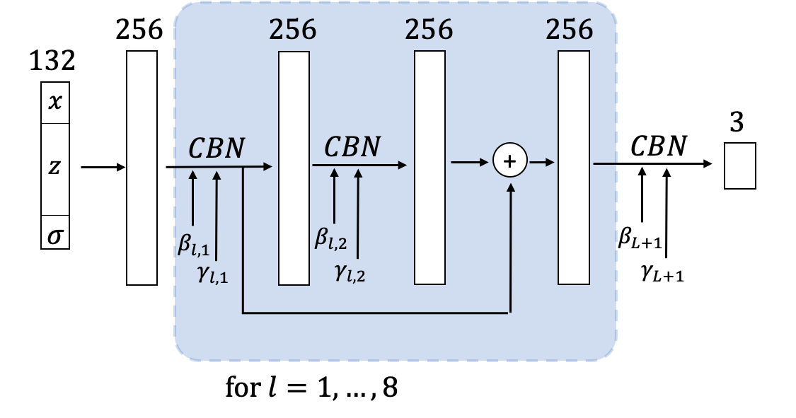
Figure 6: The gradient decoder network $s_{\theta}$. For each layer, the spatial size is specified on top. The input point $x$ is concatenated to the latent code $z$ and noise level $\sigma$. The output of $s_{\theta}$ is the gradient corresponding to the given point.

0.C.2 Experimental setting

For all the experiments, we use an Adam optimizer. We use ten different $\sigma$’s ranging from 1 to 0.01. For the ShapeNet dataset, the learning rates are $1\times 10^{-4}$ for decoder and $1\times 10^{-3}$ for encoder, with linear decay starting at 1000 epoch, reaching $1\times 10^{-5}$ and $1\times 10^{-4}$ for the encoder and the decoder, respectively. For the MNIST-CP dataset, the learning rate starts with $1\times 10^{-3}$ for both the decoder and encoder, with linear decay starting at 1000 epoch, ending at $1\times 10^{-4}$. Each batch consists of 64 shapes (or 200 shapes for the MNIST-CP dataset). We train the model for 2000 epochs. For inference, we set $T=10$ and $\alpha=2\times 10^{-4}$.

0.C.3 Baselines

In this section, we provide more details on how we obtain the reported scores for alternative methods.

PointFlow [64]

To get the results for ShapeNet, we run the pre-trained checkpoint release in the official code repository. The auto-encoding results for MNIST is obtained by running the released code on the pre-processed MNIST-CP dataset.

AtlasNet [25]

The code we used for the AtlasNet decoder comes from the official code repository. To enable a fair comparison, we use the same encoder as used in the PointFlow repository, and set the latent code dimension to be the same as our own model. We use the suggested learning rate and optimizer setting from the AtlasNet code-base and paper during training. We train AtlasNet for the same amount of iterations as our method to obtain the reported performance in Table 1 in the main paper.

l-GAN and r-GAN [2]

We modify the official released code repository to take our pre-processed point cloud from ShapeNet version 2 [7, 8]. The auto-encoding results (i.e. Table 1 in main paper) for l-GAN and r-GAN are obtained by running the official code for the same number of iterations as our model. The generation results for r-GAN in Table 3 in the main paper is obtained by running the latent-GAN in the official code for the default amount of iterations in the configuration.

GraphCNN-GAN [59]

We use the official code released in this repository to obtain the results: https://github.com/diegovalsesia/GraphCNN-GAN.

TreeGAN [52]

We use the official code released in this repository to obtain the results: https://github.com/seowok/TreeGAN.git.

Appendix 0.D Additional Quantitative Results

0.D.1 Shape generation

We compare our method’s performance on shape generation with GraphCNN-GAN [59] and TreeGAN [52] in Table 5 (in addition to the comparisons to r-GAN [1] and PointFlow [64] which we report in the main paper). As discussed in the Related Work section (Section 2 in the main paper), both of these two baselines treat generating point clouds with $N$ points as predicting a fixed dimensional vector (in practice predicting a $N\times 3$ vector but they could potentially use more upsampling layers to predict more points), using the same discriminator as r-GAN [2]. These works report performance for models trained on smaller collections (i.e. the ShapeNet Benchmark dataset) using different splits and normalization. Therefore, in addition to comparing their publicly available models (in the first rows), we retrain their models on the full ShapeNet collections using the same splits and preprocessing performed on our trained models (in the rows marked with an asterisk ($*$)). For each model, the training is performed over two days with a GeForce GTX TITAN X GPU.

Table 5: Additional shape generation results. Rows marked with an asterisk ($*$) denote retrained models. $\uparrow$ means the higher the better, $\downarrow$ means the lower the better. MMD-CD is multiplied by $10^{3}$ and MMD-EMD is multiplied by $10^{2}$.

		MMD ($\downarrow$)		COV (%, $\uparrow$)		1-NNA (%, $\downarrow$)
Category	Model	CD	EMD	CD	EMD	CD	EMD
Airplane	GCN [59]	2.623	15.535	9.38	5.93	95.16	99.12
	GCN [59]∗	44.93	35.52	1.98	1.23	99.99	99.99
	Tree [52]	1.466	16.662	44.69	6.91	95.06	100.00
	Tree [52]∗	1.798	24.723	31.60	5.43	95.43	99.88
	Ours	1.285	7.364	47.65	41.98	85.06	83.46
	Train	1.288	7.036	45.43	45.43	72.10	69.38
Chair	GCN [59]	23.098	25.781	6.95	6.34	86.52	96.48
	GCN [59]∗	140.84	0.5163	1.67	1.06	100	100
	Tree [52]	16.147	36.545	40.33	8.76	74.55	99.92
	Tree [52]∗	17.124	26.405	42.90	20.09	77.49	98.11
	Ours	14.818	18.791	46.37	46.22	66.16	59.82
	Train	15.893	18.472	50.45	52.11	53.93	54.15

We also present generation results for the car category in Table 6. Our model achieves performance that’s un-par with the state-of-the-arts.

Table 6: Shape generation results. $\uparrow$ means the higher the better, $\downarrow$ means the lower the better. MMD-CD is multiplied by $10^{3}$ and MMD-EMD is multiplied by $10^{2}$.

		MMD ($\downarrow$)			COV (%, $\uparrow$)			1-NNA (%, $\downarrow$)
Category	Model	CD	EMD		CD	EMD		CD	EMD
Car	rGAN [2]	6.233	18.561		8.24	5.11		99.29	99.86
	PF [64]	4.207	10.631		39.20	44.89		68.75	62.64
	Ours	4.085	10.610		44.60	46.88		65.48	62.93
	Train	4.207	10.631		48.30	54.26		52.98	49.57

In Figure 7, we show convergence curves for our method and for PointFlow [64] on the auto-encoding task (over the Airplane category). As the figure illustrates, our method converges much faster and to a better result.

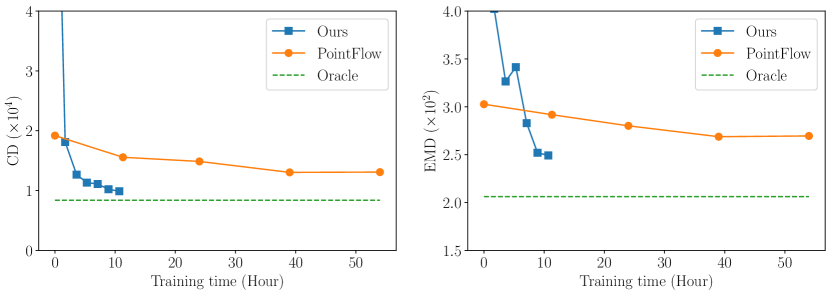
Figure 7: Convergence curves for PointFlow [64] and our method on the auto-encoding task. As illustrated above, our method converges much faster to a better result.

0.D.2 Implicit surface

Table 7: Implicit surface results on Airplane category. CD is multiplied by $10^{4}$ and EMD is multiplied by $10^{2}$.

Metrics	AtlasNet-Sph.	AtlasNet-25	DeepSDF	Ours
CD	1.88	2.16	1.43	1.022
CD (median)	0.79	0.65	0.36	0.442
EMD	3.8	4.1	3.3	5.545
Mesh acc	0.013	0.013	0.004	0.008

In this section, we demonstrate that one can use MISE [39], an octree-based marching cue algorithm, to extract a ground truth mesh that from the learned gradient field. We compute ground truth meshes for the test set of the airplane category following DeepSDF’s set-up. As mentioned in Section 1 of main paper, prior implicit representations [11][39][47] require knowing the ground truth meshes in order to provide a supervision signal during training, while our model can be trained solely from sparse point clouds. We conducted a preliminary quantitative comparison between our implicit surface and that of DeepSDF[47]. We follow DeepSDF’s experiment set-up to report results on the airplane category in Table7. Our implicit surfaces outperforms AtlasNet in both CD and Mesh accuracy metrics and are competitive with DeepSDF (which uses more supervision) in CD. Failure cases for our extracted meshes usually comes from the bifurcation area (i.e. the local minimums and saddle points) where gradients are close to zero. Another problem with our extracted surface is that marching cue tend to create a double surface around the shape, As our focus is generating point clouds, we will leave the improvement of surface extraction to future work.

Appendix 0.E Additional Ablation Studies

Next we report results of additional ablation studies to evaluating several design considerations and our choice in modeling the distribution of shapes.

Network architecture

Table 8: Architecture ablation study, comparing auto-encoding performance on the Airplane category. CD is multiplied by $10^{4}$ and EMD is multiplied by $10^{2}$. The ablated models are detailed in the text.

Metrics	(a)	(ab)	(abc)	(bd)	(abcd)
CD	1.234$\pm$0.007	0.992$\pm$0.002	0.998$\pm$0.003	1.011$\pm$0.008	0.987$\pm$0.001
EMD	2.718$\pm$0.039	2.513$\pm$0.019	2.493$\pm$0.010	2.462$\pm$0.042	2.524$\pm$0.001

We evaluate different architectures considering the following:

1. Replacing BN with CBN.

2. Adding shortcuts.

3. Replacing the latent code $z$ with $\tilde{z}=[x,z,\sigma]$ for the CBN layer.

4. Concatenating the latent code $z$ and $\sigma$ to $x$ as input for the decoder.

In Table 8 we report multiple configurations, with the rightmost one (abcd) corresponding to our full model. For each model, we perform 3 inference runs, and report the average and the standard deviation over these runs. As the table illustrates, our full model yields better performance as well as significantly smaller variance across different runs.

Modeling the distribution of shapes

In our work, we propose a new approach of modeling the distribution of points using the gradient of the log density field. To model the distribution of shapes, we use a latent GAN [1]. Next, we explore a different method to model the distribution of shapes. Specifically, we train a VAE using the same encoder and decoder setting as the one used in Section 4.2 in the main paper. We double the output dimension for the encoder so that it can output both $\mathbf{\mu}$ and $\mathbf{\sigma}$ for the re-parameterization. We add the KL-divergence loss with weight $10^{-3}$ and train for the same amount of time (in terms of epochs and iterations) as the model reported in the main paper. The results for the Chair and Airplane categories are reported in Table 9. We can see that our reported model, which uses a two-stage training with a latent-GAN, outperforms the model trained with VAE for both the Chair and the Airplane category on all metrics, except for the 1-NNA-EMD metrics on Airplane.

Table 9: Modeling the distribution of shapes using different techniques. We compare our model’s performance on the generation task against a VAE model. $\uparrow$ means the higher the better, $\downarrow$ means the lower the better. MMD-CD is multiplied by $10^{3}$ and MMD-EMD is multiplied by $10^{2}$.

		MMD ($\downarrow$)		COV (%, $\uparrow$)		1-NNA (%, $\downarrow$)
Category	Model	CD	EMD	CD	EMD	CD	EMD
Airplane	VAE	1.909	9.004	37.78	38.27	89.14	86.05
	Ours	1.332	7.768	39.01	43.46	88.52	86.91
	Train	1.288	7.036	45.43	45.43	72.10	69.38
Chair	VAE	18.032	20.903	41.99	43.81	74.17	74.92
	Ours	14.818	18.791	46.37	46.22	66.16	59.82
	Train	15.893	18.472	50.45	52.11	53.93	54.15

Appendix 0.F Additional Qualitative Results

 

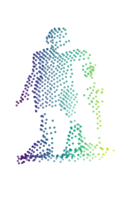
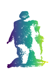
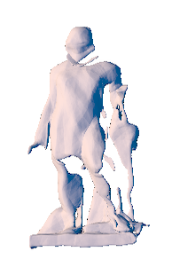
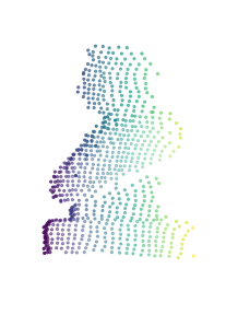
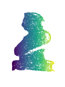
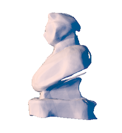
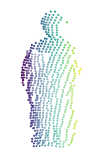
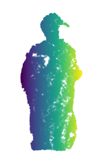
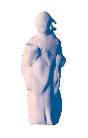
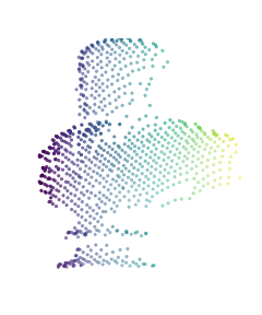
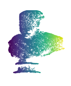
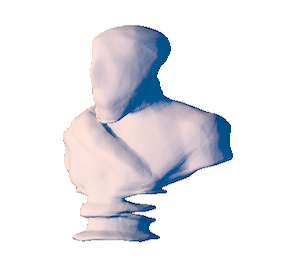
Figure 8: Autoencoding scanned shapes. Above we demonstrate our technique on sparse point clouds captured with a 3D scanner (left). We sample 10K points to obtain the point clouds illustrated in the middle and also extract the implicit surfaces (right).

Scanned data

To demonstrate that our technique can also model partial and incomplete shapes, we use scanned point clouds captured using a hand-held 3D scanner, as detailed in Yifan et al.[66]. For each scanned object, we train a separate model, evaluating to what extent we can obtain a high-fidelity point cloud reconstruction for these scanned objects. See Figure 8 for a qualitative comparison of the input scanned objects which contain roughly 600 points (left columns), reconstructed point clouds (middle columns) and extracted implicit surfaces (right columns). While we cannot model the full shape in this case (as we are only provided with a partial, single view), our technique enables reconstructing a denser representation even in this sparse real setting.

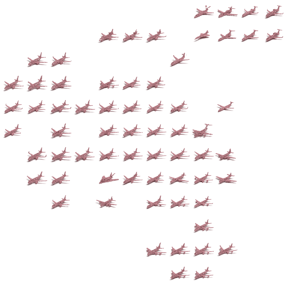
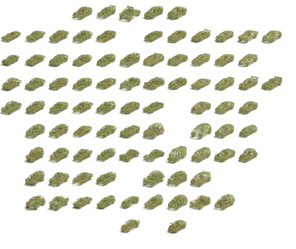
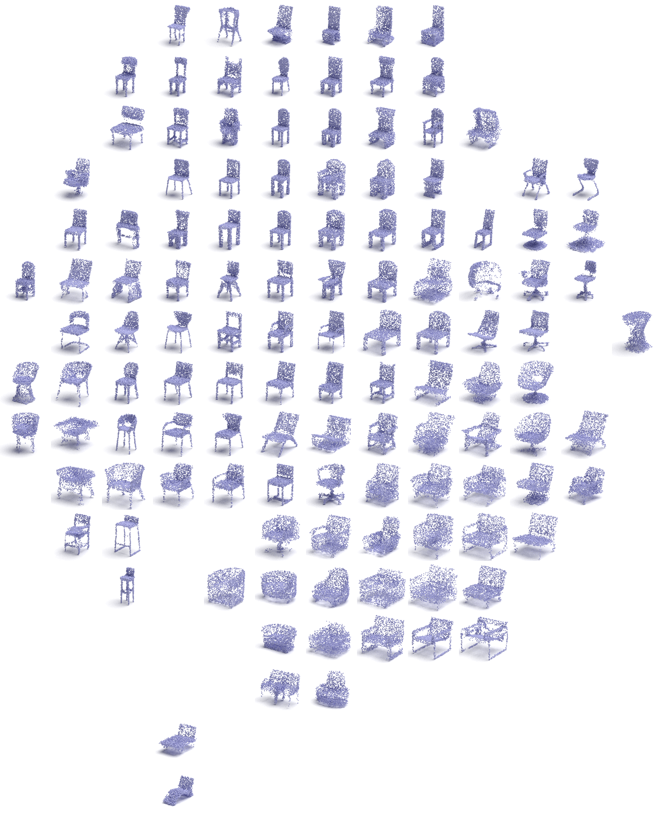
Figure 9: Visualization of the latent space.

Visualization of latent space

We visualize the latent code space in Figure 9. We first obtain all latent code $z\in\mathbb{R}^{128}$ by running the encoder on the validation set of Airplane, Car, and Chair. We run T-SNE [38] on the latent code for the same category to reduce the latent-codes’ dimensionality down to $2$. These $2$-dimensional latent codes are then used to place rendered reconstructed point clouds on the figure. The figure shows that the latent code places similar shapes nearby in the latent space, which suggests that we learn a meaningful latent space.

Extended visualizations for 2D and 3D point clouds

In Figure 10, we demonstrate our annealed Langevin dynamic procedure for 2D point clouds from MNIST-CP. We also show that our model is insensitive to the choice of the prior distribution in the 2D case in Figure 11. We show more results on the ShapeNet dataset in Figure 12 (auto-encoding shapes), Figure 13(auto-encoding point clouds), Figure 14 (shape generation), and Figure 15 (shape interpolation).

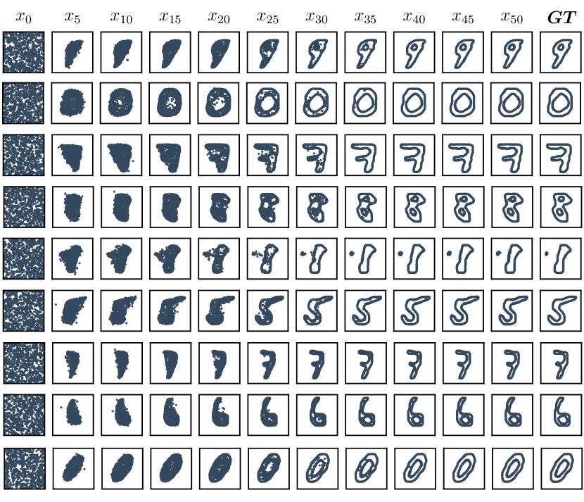
Figure 10: Point cloud sampling on the MNIST-CP dataset. Above we illustrate our annealed Langevin dynamics procedure for 2D shapes. Starting with points sampled from a uniform distribution, the points gradually move along the logarithmic density field. As illustrated on the right side, eventually these points are mostly indistinguishable from the ground truth point clouds.

sResults (different priors) sssssGT

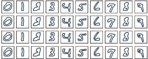
Figure 11: Reconstructing MNIST-CP shapes (illustrated on top), starting from different prior distributions. Above we demonstrate reconstruction results obtained starting from a uniform (second row), Gaussian (third row) or a single point (fourth row) distribution. As the figure illustrates, our method is insensitive to the prior distribution.

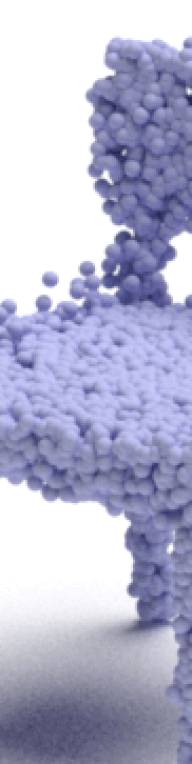
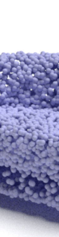
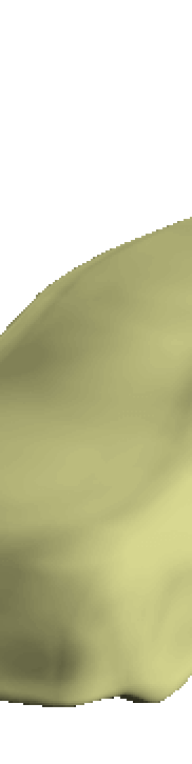
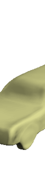
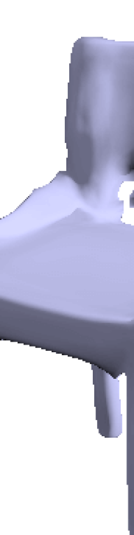
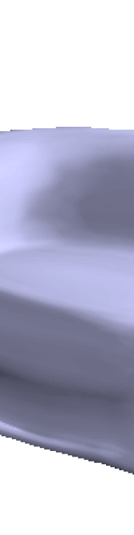
Figure 12: Examples of reconstruction results. The first row depicts reconstructed shapes from the Airplane, Car and Chair categories. The second row is the corresponding implicit surfaces.

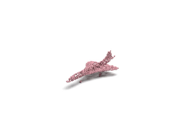
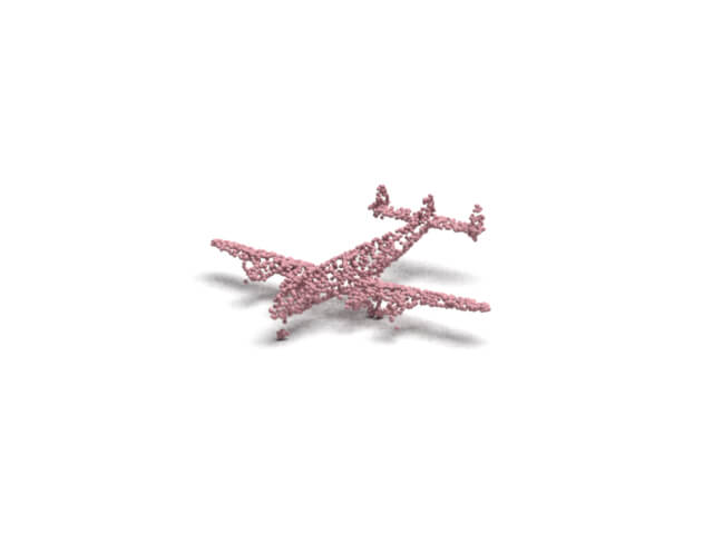
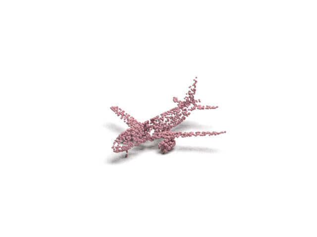
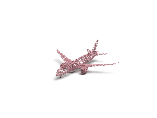
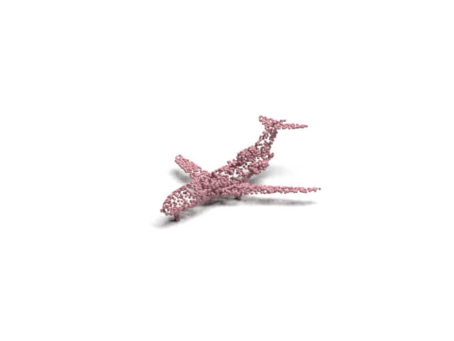
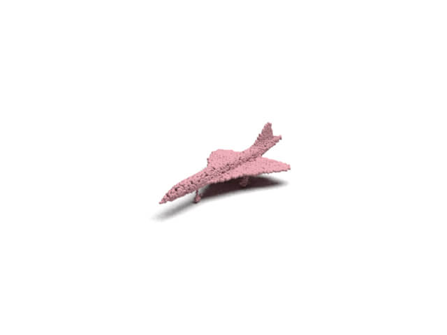
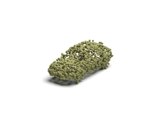
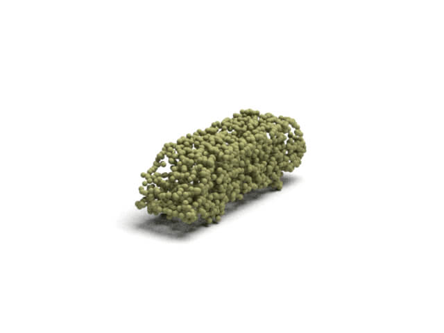
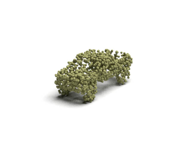
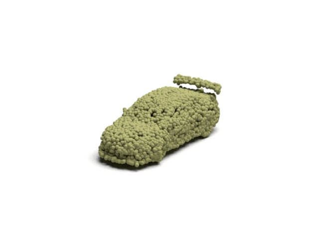
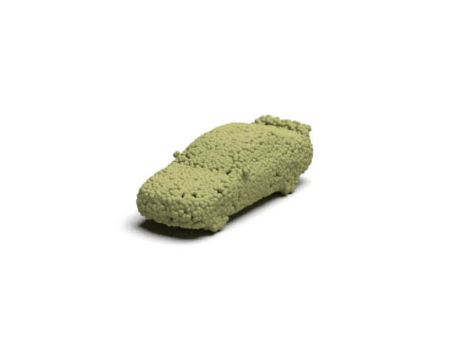
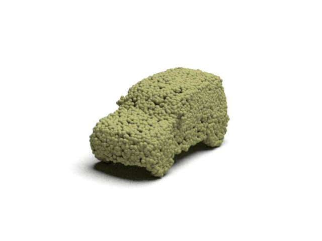
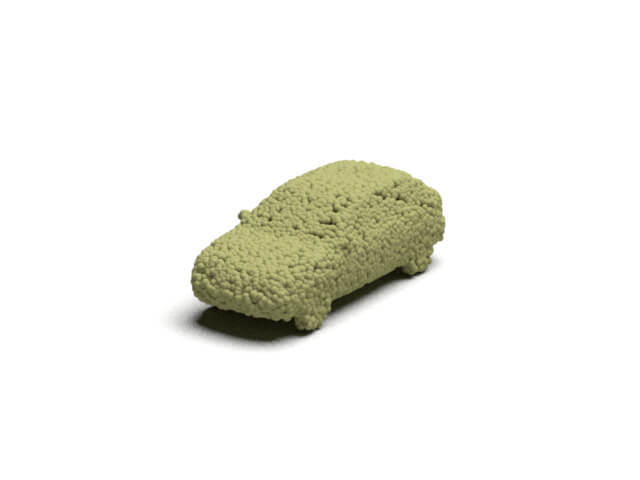
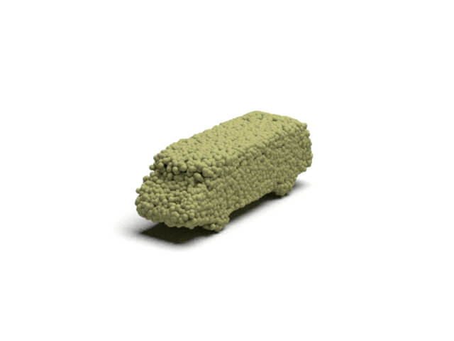
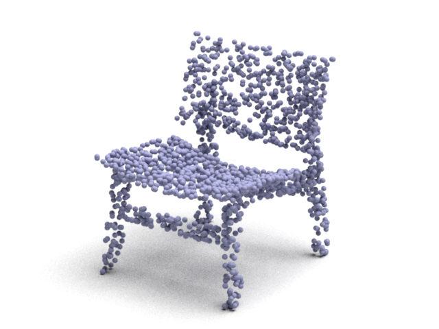
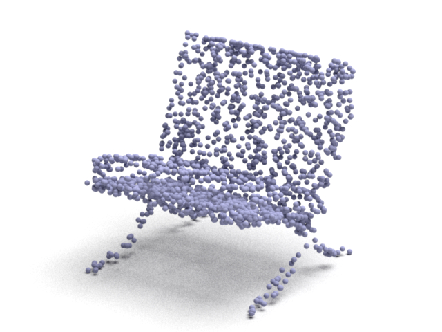
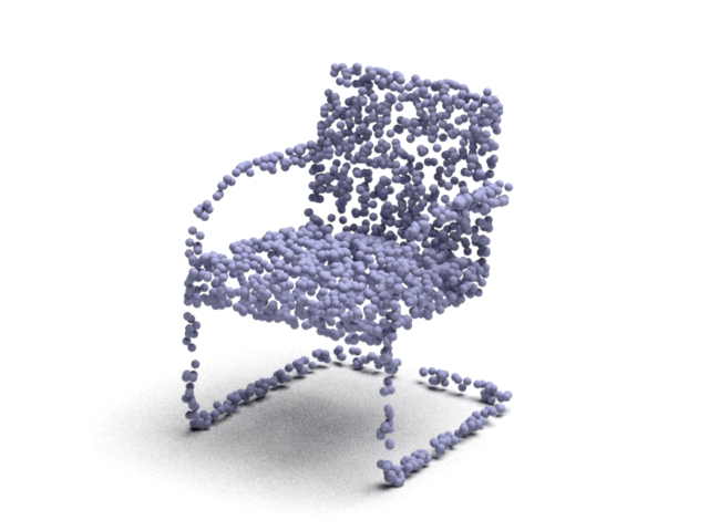
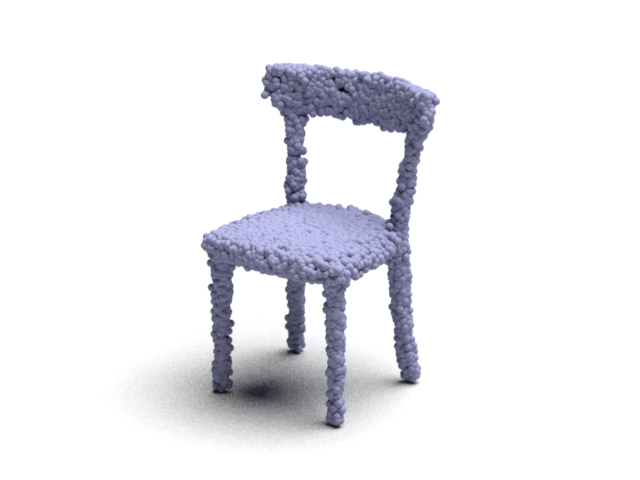
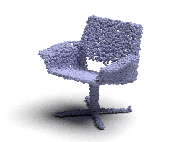
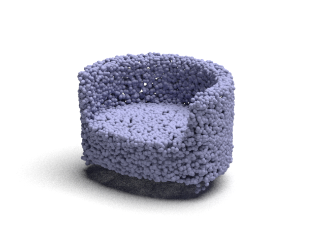
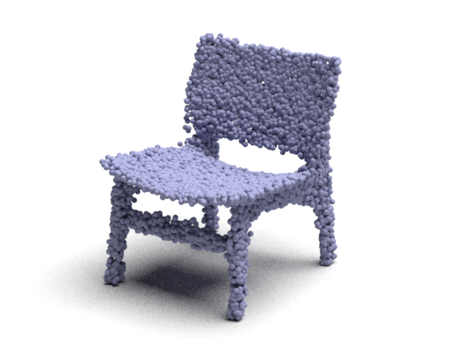
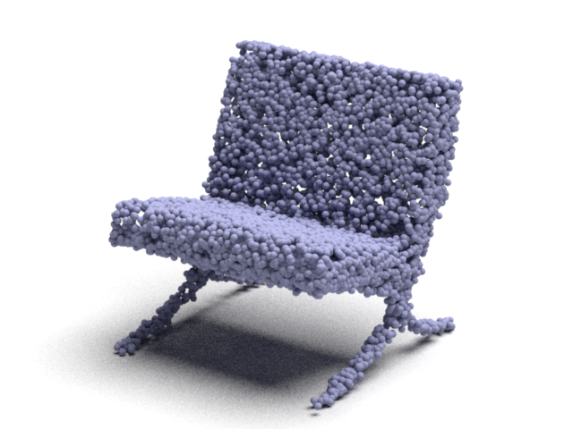
Figure 13: Examples of reconstruction results on the Airplane, Car and Chair categories. For each category, the first row is the input point cloud, and the second row is the up-sampling output point cloud.

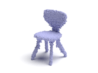
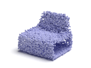
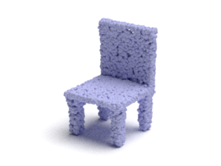
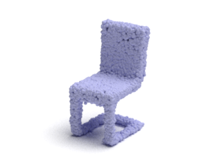
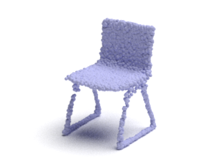
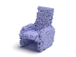
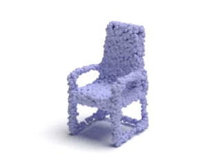
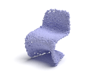
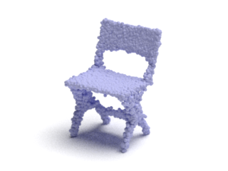
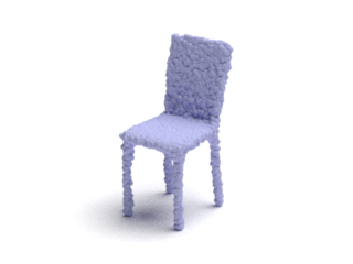
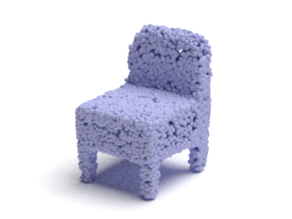
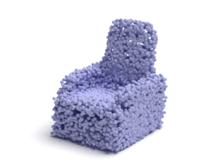
Figure 14: Examples of generation results on the Airplane, Car and Chair categories.

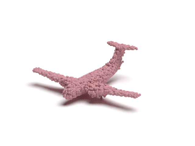
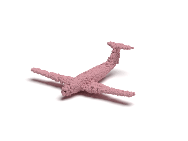
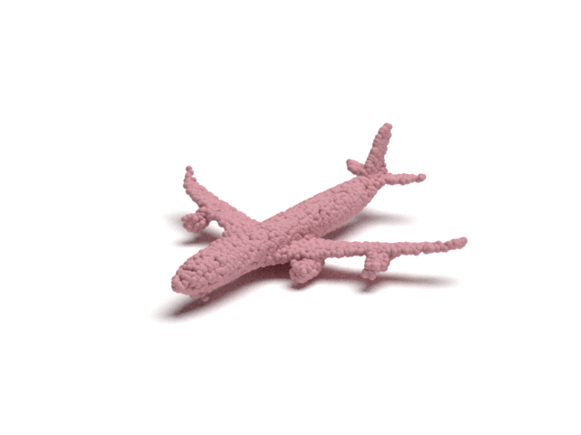
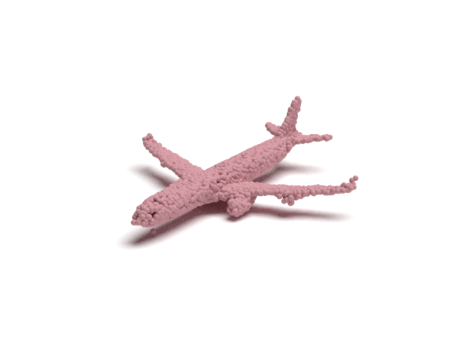
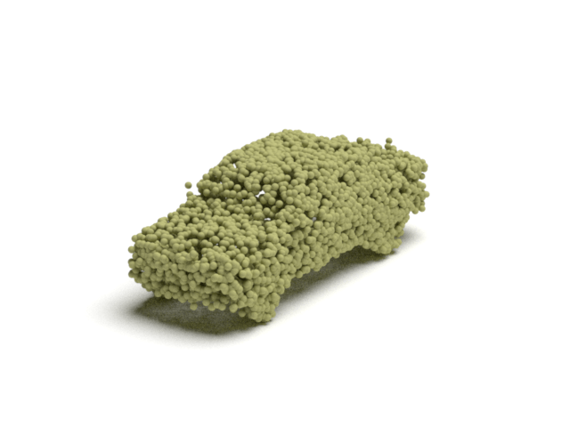
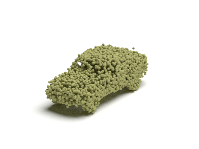
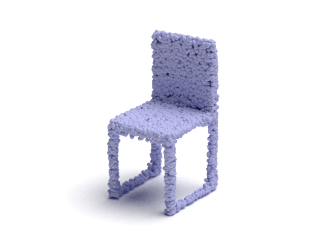
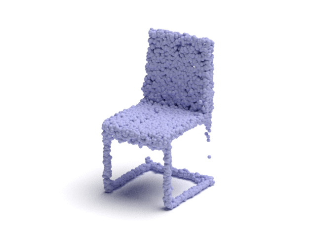
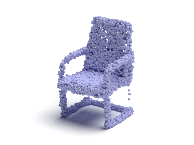
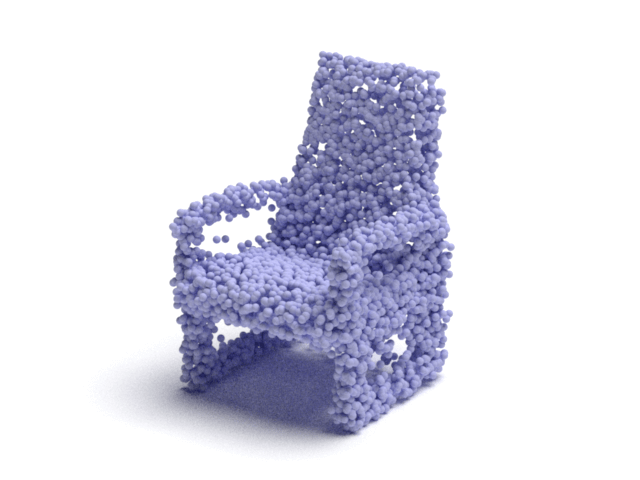
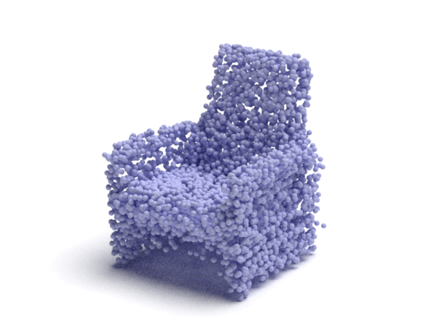
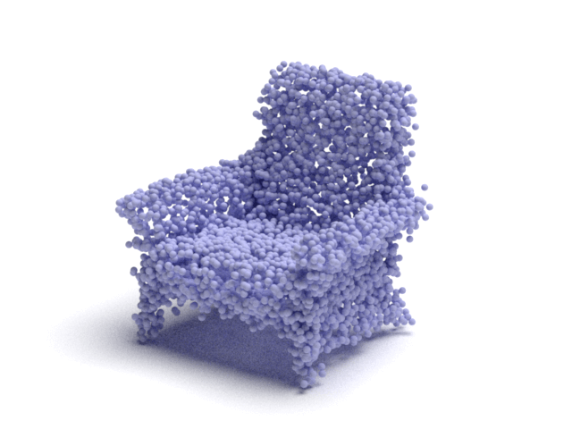
Sampled	Interp	Interp	Interp	Interp	Sampled

Figure 15: Generation and interpolation results. Generated point clouds (Sampled) and the interpolated results between two generated shapes (Interp) are illustrated.

References

- [1] Achlioptas, P., Diamanti, O., Mitliagkas, I., Guibas, L.: Learning representations and generative models for 3d point clouds. arXiv preprint arXiv:1707.02392 (2017)
- [2] Achlioptas, P., Diamanti, O., Mitliagkas, I., Guibas, L.: Learning representations and generative models for 3d point clouds. In: ICML (2018)
- [3] Anguelov, D., Srinivasan, P., Koller, D., Thrun, S., Rodgers, J., Davis, J.: Scape: shape completion and animation of people. In: ACM SIGGRAPH 2005 Papers, pp. 408–416 (2005)
- [4] Arjovsky, M., Chintala, S., Bottou, L.: Wasserstein generative adversarial networks. In: ICML (2017)
- [5] Atzmon, M., Lipman, Y.: Sal: Sign agnostic learning of shapes from raw data. In: Proceedings of the IEEE/CVF Conference on Computer Vision and Pattern Recognition. pp. 2565–2574 (2020)
- [6] Ben-Hamu, H., Maron, H., Kezurer, I., Avineri, G., Lipman, Y.: Multi-chart generative surface modeling. ACM Transactions on Graphics (TOG) 37(6), 1–15 (2018)
- [7] Chang, A.X., Funkhouser, T., Guibas, L., Hanrahan, P., Huang, Q., Li, Z., Savarese, S., Savva, M., Song, S., Su, H., Xiao, J., Yi, L., Yu, F.: ShapeNet: An Information-Rich 3D Model Repository. Tech. Rep. arXiv:1512.03012 [cs.GR], Stanford University — Princeton University — Toyota Technological Institute at Chicago (2015)
- [8] Chang, A.X., Funkhouser, T., Guibas, L., Hanrahan, P., Huang, Q., Li, Z., Savarese, S., Savva, M., Song, S., Su, H., et al.: Shapenet: An information-rich 3d model repository. arXiv preprint arXiv:1512.03012 (2015)
- [9] Chen, T.Q., Rubanova, Y., Bettencourt, J., Duvenaud, D.K.: Neural ordinary differential equations. In: NeurIPS (2018)
- [10] Chen, T., Fox, E., Guestrin, C.: Stochastic gradient hamiltonian monte carlo. In: International conference on machine learning. pp. 1683–1691 (2014)
- [11] Chen, Z., Zhang, H.: Learning implicit fields for generative shape modeling. In: Proceedings of the IEEE Conference on Computer Vision and Pattern Recognition. pp. 5939–5948 (2019)
- [12] Deprelle, T., Groueix, T., Fisher, M., Kim, V., Russell, B., Aubry, M.: Learning elementary structures for 3d shape generation and matching. In: Advances in Neural Information Processing Systems. pp. 7433–7443 (2019)
- [13] Dinh, L., Krueger, D., Bengio, Y.: Nice: Non-linear independent components estimation. CoRR abs/1410.8516 (2014)
- [14] Du, Y., Mordatch, I.: Implicit generation and generalization in energy-based models. arXiv preprint arXiv:1903.08689 (2019)
- [15] Fan, A., Fisher III, J.W., Kane, J., Willsky, A.S.: Mcmc curve sampling and geometric conditional simulation. In: Computational Imaging VI. vol. 6814, p. 681407. International Society for Optics and Photonics (2008)
- [16] Fan, A.C., Fisher, J.W., Wells, W.M., Levitt, J.J., Willsky, A.S.: Mcmc curve sampling for image segmentation. In: International Conference on Medical Image Computing and Computer-Assisted Intervention. pp. 477–485. Springer (2007)
- [17] Fan, H., Su, H., Guibas, L.J.: A point set generation network for 3d object reconstruction from a single image. In: CVPR (2017)
- [18] Gadelha, M., Wang, R., Maji, S.: Multiresolution tree networks for 3d point cloud processing. In: Proceedings of the European Conference on Computer Vision (ECCV). pp. 103–118 (2018)
- [19] Gadelha, M., Wang, R., Maji, S.: Multiresolution tree networks for 3d point cloud processing. In: ECCV (2018)
- [20] Gao, L., Yang, J., Wu, T., Yuan, Y.J., Fu, H., Lai, Y.K., Zhang, H.: Sdm-net: Deep generative network for structured deformable mesh. ACM Transactions on Graphics (TOG) 38(6), 1–15 (2019)
- [21] Genova, K., Cole, F., Sud, A., Sarna, A., Funkhouser, T.: Deep structured implicit functions. arXiv preprint arXiv:1912.06126 (2019)
- [22] Genova, K., Cole, F., Vlasic, D., Sarna, A., Freeman, W.T., Funkhouser, T.: Learning shape templates with structured implicit functions. In: Proceedings of the IEEE International Conference on Computer Vision. pp. 7154–7164 (2019)
- [23] Girdhar, R., Fouhey, D.F., Rodriguez, M., Gupta, A.: Learning a predictable and generative vector representation for objects. In: European Conference on Computer Vision. pp. 484–499. Springer (2016)
- [24] Grathwohl, W., Chen, R.T.Q., Bettencourt, J., Sutskever, I., Duvenaud, D.: Ffjord: Free-form continuous dynamics for scalable reversible generative models. In: ICLR (2019)
- [25] Groueix, T., Fisher, M., Kim, V.G., Russell, B., Aubry, M.: AtlasNet: A Papier-Mâché Approach to Learning 3D Surface Generation. In: CVPR (2018)
- [26] Gulrajani, I., Ahmed, F., Arjovsky, M., Dumoulin, V., Courville, A.C.: Improved training of wasserstein gans. In: NeurIPS (2017)
- [27] Hanocka, R., Hertz, A., Fish, N., Giryes, R., Fleishman, S., Cohen-Or, D.: Meshcnn: a network with an edge. ACM Transactions on Graphics (TOG) 38(4), 1–12 (2019)
- [28] Hao, Z., Averbuch-Elor, H., Snavely, N., Belongie, S.: Dualsdf: Semantic shape manipulation using a two-level representation. In: Proceedings of the IEEE/CVF Conference on Computer Vision and Pattern Recognition. pp. 7631–7641 (2020)
- [29] Hyvärinen, A.: Estimation of non-normalized statistical models by score matching. Journal of Machine Learning Research 6(Apr), 695–709 (2005)
- [30] Kingma, D.P., Dhariwal, P.: Glow: Generative flow with invertible 1x1 convolutions. In: NeurIPS (2018)
- [31] LeCun, Y., Chopra, S., Hadsell, R., Ranzato, M., Huang, F.: A tutorial on energy-based learning. Predicting structured data 1(0) (2006)
- [32] LeCun, Y., Cortes, C., Burges, C.: Mnist handwritten digit database (2010)
- [33] Li, C.L., Zaheer, M., Zhang, Y., Poczos, B., Salakhutdinov, R.: Point cloud gan. arXiv preprint arXiv:1810.05795 (2018)
- [34] Li, J., Xu, K., Chaudhuri, S., Yumer, E., Zhang, H., Guibas, L.: Grass: Generative recursive autoencoders for shape structures. ACM Transactions on Graphics (TOG) 36(4), 1–14 (2017)
- [35] Litany, O., Bronstein, A., Bronstein, M., Makadia, A.: Deformable shape completion with graph convolutional autoencoders. In: Proceedings of the IEEE conference on computer vision and pattern recognition. pp. 1886–1895 (2018)
- [36] Liu, Q., Lee, J., Jordan, M.: A kernelized stein discrepancy for goodness-of-fit tests. In: International conference on machine learning. pp. 276–284 (2016)
- [37] Lorensen, W.E., Cline, H.E.: Marching cubes: A high resolution 3d surface construction algorithm. ACM siggraph computer graphics 21(4), 163–169 (1987)
- [38] Maaten, L.v.d., Hinton, G.: Visualizing data using t-sne. Journal of machine learning research 9(Nov), 2579–2605 (2008)
- [39] Mescheder, L., Oechsle, M., Niemeyer, M., Nowozin, S., Geiger, A.: Occupancy networks: Learning 3d reconstruction in function space. In: Proceedings of the IEEE Conference on Computer Vision and Pattern Recognition. pp. 4460–4470 (2019)
- [40] Michalkiewicz, M., Pontes, J.K., Jack, D., Baktashmotlagh, M., Eriksson, A.: Deep level sets: Implicit surface representations for 3d shape inference. arXiv preprint arXiv:1901.06802 (2019)
- [41] Mo, K., Guerrero, P., Yi, L., Su, H., Wonka, P., Mitra, N., Guibas, L.J.: Structurenet: Hierarchical graph networks for 3d shape generation. arXiv preprint arXiv:1908.00575 (2019)
- [42] Nijkamp, E., Hill, M., Han, T., Zhu, S.C., Wu, Y.N.: On the anatomy of mcmc-based maximum likelihood learning of energy-based models. arXiv preprint arXiv:1903.12370 (2019)
- [43] Van den Oord, A., Kalchbrenner, N., Espeholt, L., Vinyals, O., Graves, A., et al.: Conditional image generation with pixelcnn decoders. In: NeurIPS (2016)
- [44] Oord, A.v.d., Dieleman, S., Zen, H., Simonyan, K., Vinyals, O., Graves, A., Kalchbrenner, N., Senior, A., Kavukcuoglu, K.: Wavenet: A generative model for raw audio. arXiv preprint arXiv:1609.03499 (2016)
- [45] Oord, A.v.d., Kalchbrenner, N., Kavukcuoglu, K.: Pixel recurrent neural networks. In: ICML (2016)
- [46] Papamakarios, G., Nalisnick, E., Rezende, D.J., Mohamed, S., Lakshminarayanan, B.: Normalizing flows for probabilistic modeling and inference. arXiv preprint arXiv:1912.02762 (2019)
- [47] Park, J.J., Florence, P., Straub, J., Newcombe, R., Lovegrove, S.: Deepsdf: Learning continuous signed distance functions for shape representation. In: Proceedings of the IEEE Conference on Computer Vision and Pattern Recognition. pp. 165–174 (2019)
- [48] Pons-Moll, G., Romero, J., Mahmood, N., Black, M.J.: Dyna: A model of dynamic human shape in motion. ACM Transactions on Graphics (TOG) 34(4), 1–14 (2015)
- [49] Qi, C.R., Su, H., Mo, K., Guibas, L.J.: Pointnet: Deep learning on point sets for 3d classification and segmentation. In: CVPR (2017)
- [50] Rezende, D.J., Mohamed, S.: Variational inference with normalizing flows. In: ICML (2015)
- [51] Roth, S.D.: Ray casting for modeling solids. Computer graphics and image processing 18(2), 109–144 (1982)
- [52] Shu, D.W., Park, S.W., Kwon, J.: 3d point cloud generative adversarial network based on tree structured graph convolutions. In: Proceedings of the IEEE International Conference on Computer Vision. pp. 3859–3868 (2019)
- [53] Smirnov, D., Fisher, M., Kim, V.G., Zhang, R., Solomon, J.: Deep parametric shape predictions using distance fields. arXiv preprint arXiv:1904.08921 (2019)
- [54] Song, Y., Ermon, S.: Generative modeling by estimating gradients of the data distribution. In: Advances in Neural Information Processing Systems. pp. 11895–11907 (2019)
- [55] Song, Y., Garg, S., Shi, J., Ermon, S.: Sliced score matching: A scalable approach to density and score estimation. arXiv preprint arXiv:1905.07088 (2019)
- [56] Sun, Y., Wang, Y., Liu, Z., Siegel, J.E., Sarma, S.E.: Pointgrow: Autoregressively learned point cloud generation with self-attention. arXiv preprint arXiv:1810.05591 (2018)
- [57] Tan, Q., Gao, L., Lai, Y.K., Xia, S.: Variational autoencoders for deforming 3d mesh models. In: Proceedings of the IEEE conference on computer vision and pattern recognition. pp. 5841–5850 (2018)
- [58] Tulsiani, S., Su, H., Guibas, L.J., Efros, A.A., Malik, J.: Learning shape abstractions by assembling volumetric primitives. In: Proceedings of the IEEE Conference on Computer Vision and Pattern Recognition. pp. 2635–2643 (2017)
- [59] Valsesia, D., Fracastoro, G., Magli, E.: Learning localized generative models for 3d point clouds via graph convolution (2018)
- [60] Vincent, P.: A connection between score matching and denoising autoencoders. Neural computation 23(7), 1661–1674 (2011)
- [61] Welling, M., Teh, Y.W.: Bayesian learning via stochastic gradient langevin dynamics. In: Proceedings of the 28th international conference on machine learning (ICML-11). pp. 681–688 (2011)
- [62] Wenliang, L., Sutherland, D., Strathmann, H., Gretton, A.: Learning deep kernels for exponential family densities. arXiv preprint arXiv:1811.08357 (2018)
- [63] Wu, J., Zhang, C., Xue, T., Freeman, B., Tenenbaum, J.: Learning a probabilistic latent space of object shapes via 3d generative-adversarial modeling. In: Advances in neural information processing systems. pp. 82–90 (2016)
- [64] Yang, G., Huang, X., Hao, Z., Liu, M.Y., Belongie, S., Hariharan, B.: Pointflow: 3d point cloud generation with continuous normalizing flows. In: Proceedings of the IEEE International Conference on Computer Vision. pp. 4541–4550 (2019)
- [65] Yang, Y., Feng, C., Shen, Y., Tian, D.: Foldingnet: Point cloud auto-encoder via deep grid deformation. In: CVPR (2018)
- [66] Yifan, W., Wu, S., Huang, H., Cohen-Or, D., Sorkine-Hornung, O.: Patch-based progressive 3d point set upsampling. In: Proceedings of the IEEE Conference on Computer Vision and Pattern Recognition. pp. 5958–5967 (2019)
- [67] Zamorski, M., Zieba, M., Nowak, R., Stokowiec, W., Trzcinski, T.: Adversarial autoencoders for generating 3d point clouds. arXiv preprint arXiv:1811.07605 2 (2018)
- [68] Zamorski, M., Zieba, M., Nowak, R., Stokowiec, W., Trzciński, T.: Adversarial autoencoders for generating 3d point clouds. arXiv preprint arXiv:1811.07605 (2018)