The early discovery of SN 2017ahn: signatures of persistent interaction in a fast declining Type II supernova

Abstract

We present high-cadence, comprehensive data on the nearby ($D\simeq 33\,\rm{Mpc}$) Type II SN 2017ahn, discovered within $\sim$1 day of explosion, from the very early phases after explosion to the nebular phase. The observables of SN 2017ahn show a significant evolution over the $\simeq 470\,\rm{d}$ of our follow-up campaign, first showing prominent, narrow Balmer lines and other high-ionization features purely in emission (i.e. flash spectroscopy features), which progressively fade and lead to a spectroscopic evolution similar to that of more canonical Type II supernovae. Over the same period, the decline of the light curves in all bands is fast, resembling the photometric evolution of linearly declining H-rich core-collapse supernovae. The modeling of the light curves and early flash spectra suggest a complex circumstellar medium surrounding the progenitor star at the time of explosion, with a first dense shell produced during the very late stages of its evolution being swept up by the rapidly expanding ejecta within the first $\sim 6\,\rm{d}$ of the supernova evolution, while signatures of interaction are observed also at later phases. Hydrodynamical models support the scenario in which linearly declining Type II supernovae are predicted to arise from massive yellow super/hyper giants depleted of most of their hydrogen layers.

1 Introduction

Core-collapse supernovae (CC SNe) are the spectacular endpoint of the evolution of massive stars ($>8-9$ M_☉; Heger et al., 2003; Smartt, 2009). Hydrogen-rich SNe are typically labelled as Type II SNe (Filippenko, 1997; Gal-Yam, 2017), further classified on the basis of their photometric evolution after peak (Barbon et al., 1979; Smith et al., 2011; Li et al., 2011; Graur et al., 2017), distinguishing between transients showing a characteristic plateau lasting $\simeq 100\,\rm{d}$ (see, e.g., Anderson et al., 2014) and those showing linear, or almost linear declines after maximum light (see, e.g, Faran et al., 2014, and references therein). Although this diversity might be solely due to different amounts of H retained at the time of the explosion, different progenitor channels have been proposed for the rare class of SNe IIL ($6-10$% of all CC SNe; Smith et al., 2011; Li et al., 2011) and the more common Type IIP SNe. In particular, Type IIL have been proposed to arise from more massive stars, partially depleted of their outer H layers, with larger radii (a few $10^{3}$ R_☉; e.g., Blinnikov & Bartunov, 1993) with respect to more compact ($<1600$ R_☉; Levesque et al., 2005) and less massive red supergiants (RSGs) (see, e.g., Elias-Rosa et al., 2010; Fraser et al., 2010; Anderson et al., 2012), although Morozova et al. (2017) showed that RSGs surrounded by a dense CSM can also produce the observables of SNe IIL. On the other hand, more recently, a few authors proposed Type II SNe to form a heterogeneous class, with their light curves forming a continuum of properties (Anderson et al., 2014; Sanders et al., 2015; Galbany et al., 2016; Rubin & Gal-Yam, 2016; Valenti et al., 2016; de Jaeger et al., 2019).

CC SNe interacting with a dense H-rich circumstellar medium (CSM) typically show narrow features (with a full–width–at–half–maximum – FWHM of a few $10^{2}$ up to a few $10^{3}$ km s^-1) and are therefore labelled as SNe IIn (Schlegel, 1990). These are recombination lines emitted by the outer un-shocked CSM, with ionizing photons produced in the underlying shocked regions (see Chevalier & Fransson, 1994). Narrow lines, on the other hand, are not the only signature of ongoing ejecta-CSM interaction, as collisions between dense shells are expected to produce boxy, flat topped profiles (see, e.g., Inserra et al., 2011; Jerkstrand, 2017, and references therein), and strong signatures of interaction can be deduced from observations in the X-ray and radio domains of transients not showing narrow emission features (see, e.g., Fransson et al., 1996).

Figure 1: Color image of SN 2017ahn and its host galaxy NGC 3318. The image combined $g-$, $r-$ and $i-$band data obtained on 2017 April 16 ($\sim 68\,\rm{d}$ days after explosion) with a $1\,\rm{m}$ telescope of the Las Cumbres Observatory network (1m-012, node at the South African Astronomical Observatory – SAAO, Cape Town, South Africa). SN 2017ahn is the bright source in the middle of the inset.

While in “normal” CC SNe the SN shock is expected to break through the stellar photosphere, in stars exploding within a dense medium this typically occurs within the CSM (see, e.g., Svirski et al., 2012; Förster et al., 2018), leading to a drastic increase in the time scale of the shock breakout signal (Balberg & Loeb, 2011). While this signal typically fades within seconds to a fraction of an hour after explosion, in SNe interacting with a dense CSM this can be extended up to a time scale of days (Balberg & Loeb, 2011). This is the case of Type IIn SNe, where the shock can break through the extended CSM up to a hundred of days after the SN explosion (see, e.g., Tartaglia et al., 2020), as long as the optical depth of the overlying medium is larger than $\simeq c/v$ (where $v$ is the shock expansion velocity). After this time, their photometric evolution is mainly shaped by ongoing ejecta-CSM interaction, depending on the efficiency in the conversion of kinetic energy into radiation and the density profiles of the SN ejecta and shocked gas (see Chevalier, 1982; Moriya et al., 2013; Fransson et al., 2014). Similarly, their spectroscopic evolution can be dominated by interaction up to many years after the SN explosion, with line profiles shaped by electron scattering (see Huang & Chevalier, 2018) or, occasionally, showing emission components from shocked shells (see, e.g., Taddia et al., 2020). Interaction can mask the underlying ejecta, preventing us from collecting information about the progenitor stars (typically accessible during the nebular phases) and, occasionally, even explosion mechanisms (see, e.g., Silverman et al., 2013). This is mainly because of the pseudo photosphere being typically located in the outer un-shocked CSM, produced through stationary winds or eruptive events throughout the evolution of the progenitor star, and only reflecting the composition of the most outer layers of its envelope.

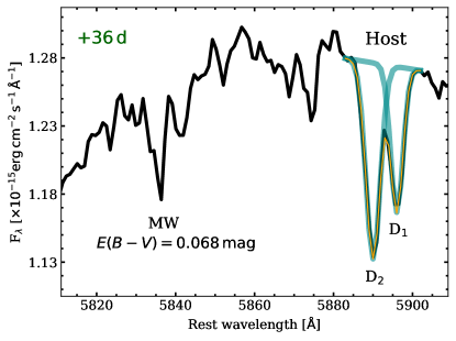
Figure 2: Zoom-in of the $5820-5900$ Å region of the spectrum obtained on 2017 March 15 ($36\,\rm{d}$ after explosion). Galactic Na ID and host absorption features are clearly visible. A multi-gaussian fit (yellow line) of the marginally resolved host features including the single components (cyan lines). The spectrum is corrected for the recessional velocity of SN 2017ahn.

On the other hand, in CC SNe discovered soon after explosion, narrow features may arise from shells expelled during the very late phases of the evolution of their progenitors, and hence reflect the chemical composition of their outer layers just before explosion (see, e.g., the cases of SNe 1983K; Niemela et al. 1985 1993J; Garnavich & Ann 1994; Matheson et al. 2000, 1998S; Leonard et al. 2000; Shivvers et al. 2015, 2006bp Quimby et al. 2007, and the more recent cases of SNe 2013cu; Gal-Yam et al. 2014, 2013fs; Yaron et al. 2017 and 2016bkv; Hosseinzadeh et al. 2018). These high ionization (e.g., He II, C III-IV, N IV-V and occasionally O IV-VI) features – sometimes dubbed ‘flash spectroscopy’ features – rapidly fade and typically disappear after a few days, depending on the physical conditions of the emitting shell, and on the time these regions are overtaken by the rapidly expanding SN ejecta. The occurrence of CC SNe showing early high-ionization features is expected to be relatively high ($\sim 20$% among those discovered within $5\,\rm{d}$ since explosion; Khazov et al., 2016) and their numbers will increase with the advent of modern $\sim$1 day cadence SN surveys such as the Palomar Transient Facility (PTF and its continuation iPTF; Law et al., 2009; Kulkarni, 2013), the All Sky Automated Survey for SNe (ASAS-SN; Shappee et al., 2014), the Asteroid Terrestrial-Impact Last Alert System (ATLAS; Tonry, 2011; Smith et al., 2020), the Distance Less Than $40\,\rm{Mpc}$ (DLT40; Tartaglia et al., 2018) and the Zwicky Transient Facility (ZTF; Graham et al., 2019; Bellm et al., 2019).

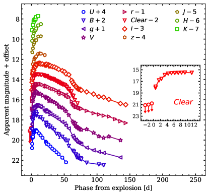
Figure 3: Optical and NIR light curves of SN 2017ahn. $U,B,V,Clear,J,H,K$ and $g,r,i,z$ magnitudes were calibrated to the Vega and AB photometric systems, respectively. Magnitudes were not corrected for the foreground Galactic or host extinction. Phases refer to the estimated epoch of the explosion. In the inset, a zoom-in shows the last non-detection limits and the early evolution of the DLT40 data.

In this context, we present the discovery and the detailed follow-up campaign of the Type II SN 2017ahn. SN 2017ahn was discovered on 2017 February 8.29 UT (Tartaglia et al., 2017) in the nearby galaxy NGC 3318 during the second year of operations of DLT40, specifically looking for nearby SNe within one day from explosion. It was given an internal designation of DLT17h. First detection and the subsequent confirmation image were both obtained using the $0.41\,\rm{m}$ PROMPT 5 telescope (Reichart et al., 2005) located at the Cerro Tololo Inter-American Observatory (CTIO, Cerro Pachón, Chile). SN 2017ahn was also observed at radio frequencies on 2017 February 28.6 UT ($\rm{JD}=2457813.1$, $\simeq 21\,\rm{d}$ after explosion) with the Australia Telescope Compact Array (ATCA), resulting in non-detection limits of 75 and $40\,\rm{\mu Jy}\,\rm{beam^{-1}}$ at 5.5 and $9.0\,\rm{GHz}$, respectively (Ryder et al., 2017). Further details about the DLT40 survey during the time period of this SN discovery are discussed in Yang et al. (2017); Tartaglia et al. (2018); Yang et al. (2019).

In Section 2 we discuss the local environment of SN 2017ahn, and infer its host extinction, while Section 3 includes details about the photometric (3.1) and spectroscopic (3.2 and 3.3) follow-up campaigns of SN 2017ahn. In Section 4, we discuss the main observables in the context of young nearby CC SNe, while the main results of our analysis are summarized in Section 5. Additional information about the facilities used to collect data as well as the reduction steps and tools are reported in the Appendix.

2 The local environment

SN 2017ahn is located at $\rm{RA}=10$:37:17.45, $\rm{Dec}=-41$:37:05.27 [J2000], 21$\farcs$75 E, 33$\farcs$93 N from the center of its host galaxy, NGC 3318 (see Figure 1). NGC 3318 is a nearby ($D\lesssim 38\,\rm{Mpc}$) spiral galaxy (SAB(rs)b; de Vaucouleurs et al., 1991), which already hosted the Type II SN 2000cl (Chassagne et al., 2000), 15$\farcs$47 W, 42$\farcs$51 S away from the position of SN 2017ahn and the Type II SN 2020aze (24$\farcs$44 W, 23$\farcs$65 S from SN 2017ahn; Ailawadhi et al. in preparation). In the following, we will assume a luminosity distance of $33.0\pm 6.5\,\rm{Mpc}$ to NGC 3318, corresponding to a distance modulus of $\mu=32.59\pm 0.43\,\rm{mag}$ (as derived by Sorce et al. 2014 using data obtained during the observational campaign Cosmicflows with Spitzer; Courtois & Tully 2012a, b; Tully & Courtois 2012; Tully et al. 2013), placing SN 2017ahn at a projected distance of $\simeq 6.4\,\rm{kpc}$ from the center of NGC 3318. This value is in agreement with that found by Carrick et al. (2015), resulting in a “cosmicflows-3” luminosity distance $D_{L}=40.76\,\rm{Mpc}$ (assuming $\Omega_{M}=0.3$, $\Omega_{\Lambda}=0.7$ and $H_{0}=70\,\rm{km}\,\rm{s^{-1}}\,\rm{Mpc^{-1}}$), corresponding to a distance modulus $\mu=33.05\pm\,\rm{mag}$, as well as that inferred using The Extragalactic Distance Database (EDD; see Kourkchi et al. 2020) based on the linear density field model of Graziani et al. (2019, $\mu=32.73\pm 0.21\,\rm{mag}$.).

For the foreground Galactic extinction we adopt the values reported by Schlafly & Finkbeiner (2011), corresponding to $E(B-V)=0.068\,\rm{mag}$, while to estimate the local extinction, we compared results obtained using different methods.

A first estimate was obtained using data collected with the VLT/Multi Unit Spectroscopic Explorer (MUSE; Bacon et al., 2014) integral field spectrograph on 2015 May 17, as part of a survey of nearby SN explosion sites (see Kuncarayakti et al., 2018, for details), which serendipitously included the site of SN 2017ahn in its field of view. Line-of-sight extinction was estimated from the observed Balmer decrement (H$\alpha$/H$\beta$, after correcting the spectrum for the Galactic extinction) of a nearby H II region, assuming an intrinsic flux ratio of 2.86 (Case B recombination; Osterbrock & Ferland, 2006) and a standard extinction law with $R_{V}=3.1$ (Cardelli et al., 1989), yielding an additional contribution of $E(B-V)=0.09\pm 0.06\,\rm{mag}$ from the local environment.

On the other hand, a rapid inspection of the $5800-6000$ Å region in our spectrum obtained on 2017 March 15 ($36\,\rm{d}$ after explosion, see Section 3) reveals host Na ID features much stronger than the those due to the Galactic extinction, with a total equivalent width $\rm{EW_{host}}\simeq 2.6\times\rm{EW_{MW}}$, as measured from the overall profile including both lines (see Figure 2). This ratio would suggest an additional contribution of $\rm{E(B-V)\simeq 0.18\,\rm{mag}}$ (assuming a standard extinction law) of the local environment to the total reddening. Since at this phase the feature is marginally resolved, we fit its profile using a combination of two gaussian centered at the position of the D2 and D1 Na ID lines (see Figure 2). The fit gives parameters for both absorption features, including their EWs, resulting in $\simeq 0.53$ and $\simeq 0.33$ Å for D2 and D1, respectively. These are both within the linearity range of the relation between the sodium EW and dust extinction derived by Poznanski et al. (2012) (see their Figure 9). Taking a weighted average between the quantities inferred using their Equations 7 and 8, these correspond to a contribution of $E(B-V)=0.196\pm 0.054\,\rm{mag}$ to the total reddening. A similar result ($E(B-V)\simeq 0.12\,\rm{mag}$) is obtained using the relations found by Turatto et al. (2003, see also ).

In order to avoid possible projection effects (SN 2017ahn lies at a projected distance of $\simeq 160\,\rm{pc}$ from the center of the H II region, assuming a distance of $33\,\rm{Mpc}$), we therefore favor $E(B-V)=0.196\,\rm{mag}$ as the contribution of the local environment to the total color excess in the direction of SN 2017ahn. This value has to be summed to the Galactic reddening in the direction of SN 2017ahn, resulting in a total extinction $E(B-V)=0.264\pm 0.054\,\rm{mag}$, although we cannot rule out a lower extcintion value (see Section 4.3). In addition, as shown by Phillips et al. (2013), these relations largely underestimate errors on the derived values, and hence the uncertainty on the reddening is probably larger.

3 Evolution of the main observables

3.1 Light curves

Optical and NIR light curves are shown in Figure 3, while the corresponding magnitudes and a description of the facilities used and reduction steps are reported in Appendix A.

The explosion epoch was estimated from the unfiltered light curve obtained with PROMPT5 (see the inset in Figure 3), taking the mid-point between the discovery (2017 February 8.29 UT; $\rm{JD}=2457792.79$) and the last non-detection limit ($m>20.8\,\rm{mag}$ on 2017 February 7.23 UT; $\rm{JD}=2457791.73$). In the following, we will therefore assume 2017 February 7.76 UT ($\rm{JD}=2457792.26\pm 0.5$) as the explosion epoch for SN 2017ahn, and refer phases to this date.

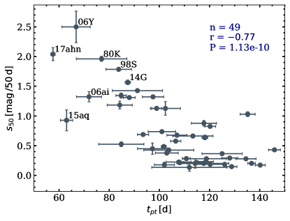
Figure 4: $V-$band decline rate measured at $+50\,\rm{d}$ ($s_{50}$) vs. $t_{pt}$ (see the main text) for the sample of Type II SNe of Valenti et al. (2016), including SN 2017ahn and SN 1998S. n is the number of objects in the sample, r the Pearson $s-$correlation coefficient and P the probability of getting a correlation by chance.

Optical light curves show a relatively fast rise to maximum (see, e.g., Anderson et al., 2014; Gall et al., 2015; González-Gaitán et al., 2015; Valenti et al., 2016) in all bands, with an average rate of $\sim 0.8\,\rm{mag}\,\rm{d^{-1}}$. Fitting high order polynomials, we infer $t_{rise}=t_{max}-t_{expl}$ ranging from $6.38\pm 0.66\,\rm{d}$ in $U$ to $8.03\pm 0.71\,\rm{d}$ in $V$, with a similar behavior in $griz$ ($8.54\pm 2.24\,\rm{d}\leq t_{rise}\leq 14.04\pm 3.99\,\rm{d}$). Errors were estimated performing Monte Carlo simulations, randomly shifting the photometric data within their uncertainties, including that on the estimated epoch of the explosion.

After peak, light curves settle on a short plateau, lasting $\simeq 50\,\rm{d}$, more pronounced at redder wavelengths, except for the $U-$band, declining linearly (with a rate of $0.069\pm 0.001\,\rm{mag}\,\rm{d^{-1}}$). At $t\gtrsim+70\,\rm{d}$, the optical light curves settle on a tail, with a slower decline at an average rate of $\simeq 0.02\,\rm{mag}\,\rm{d^{-1}}$, with the exception of the $B-$band light curve, showing a late decline of $\simeq 0.01\,\rm{mag}\,\rm{d^{-1}}$. This suggests a luminosity evolution faster than that predicted by the radioactive ${}^{56}\rm{Co}$ decay (see Section 4). Following Valenti et al. (2016) we infer a decline rate $s_{50,V}=2.04\pm 0.11\,\rm{mag}\,50\,\rm{d^{-1}}$ and a mid-point between the end of the plateau and the onset of radioactive tail $t_{pt,V}=57.56\pm 0.88\,\rm{d}$. These are similar to other fast declining Type II SNe such as SNe 1980K, 2006Y (Anderson et al., 2014), 2014G (Terreran et al., 2016) and 1998S (Fassia et al., 2000) (see Figure 4).

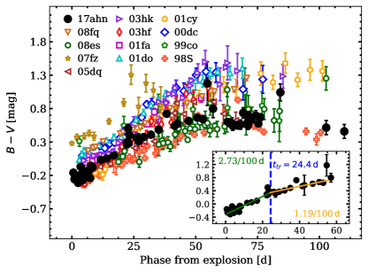
Figure 5: $B-V$ color curve of SN 2017ahn compared to the color evolution of the sample of Faran et al. (2014). The $B-V$ color evolution of SN 1998S is also included for comparison. Magnitudes were corrected for the total (Galactic+host) extinction.

In Figure 5, we compare the $B-V$ colors of SN 2017ahn to those of the sample of similarly fast declining Type II SNe of Faran et al. (2014). The resulting evolution is consistent with the bluer end of the distribution, corresponding to colors similar to those shown by SNe 1999co and 1998S, suggesting a higher temperature for the pseudo-photosphere, as will be discussed in the following sections. Following Patat et al. (1994), we identify two ‘regimes’ with different slopes in the $B-V$ color evolution. Fitting linear relations, we find an initial evolution towards redder color with a slope of $2.73\pm 0.06\,\rm{mag}\,100\,\rm{d^{-1}}$, followed by a slower evolution with a rate of $1.19\pm 0.09\,\rm{mag}\,100\,\rm{d^{-1}}$ with a break occurring at $t_{tr}\simeq+24.4\,\rm{d}$. These slopes are both steeper, with a break in the color evolution of SN 2017ahn occurring slightly earlier than the median values found for the sample of Type II SN of de Jaeger et al. (2018, $s_{1,(B-V)}\simeq 2.63$ and $s_{2,(B-V)}\simeq 0.77\,\rm{mag}\,100\,\rm{d^{-1}}$, respectively, with $t_{tr}\simeq 37.7\,\rm{d}$). At $t\gtrsim+75\,\rm{d}$ we note a further flattening, with $B-V$ colors remaining roughly constant throughout the remaining $\simeq 25\,\rm{d}$ of photometric coverage.

Assuming the distance modulus and total reddening reported in Section 2, we infer absolute peak magnitudes ranging from $M_{z}=-17.81\pm 0.29\,\rm{mag}$ to $M_{U}=-19.08\pm 0.29$ (with $M_{V}=-18.44\pm 0.29$), where the errors are dominated by the uncertainty on the distance modulus and extinction (see Section 2).

A comparison with other transients showing similar photometric properties, based on the results reported above (see Figure 6), reveals an evolution of the absolute $V-$band magnitude similar to that of SN 1998S (Fassia et al., 2000; Liu et al., 2000), which, despite the systematically brighter magnitudes and a slightly different rise time, shows the same relatively short plateau, with a comparable fast decline at $t\gtrsim+70\,\rm{d}$ ($0.002\pm 0.03\,\rm{mag}\,\rm{d^{-1}}$).

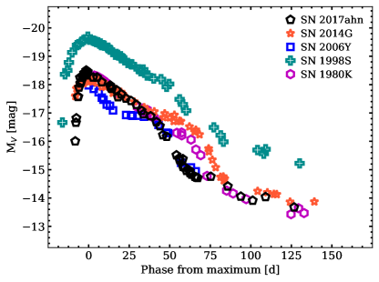
Figure 6: Absolute $V-$band light curve of SN 2017ahn compared to those of other transients showing a similar photometric evolution (see the main text).

Given the similarities in the photometric evolution of SN 2017ahn and SN 1998S and the limited coverage of our NIR light curves, we cannot rule-out the presence of an IR excess similar to those typically observed in long-lasting Type IIn SNe (see, e.g., Gerardy et al., 2002; Fox et al., 2011) and in SN 1998S itself (see Pozzo et al., 2004). These features are often explained either as ‘light echoes’ by pre-existing dust (see, e.g., Tartaglia et al., 2020) or newly formed dust in the post-shocked regions (e.g., Smith et al., 2012). On the other hand, the absence of colder components in the NIR spectral continuum of SN 2017ahn seems to suggest a lack of a clear IR excess at least until $+65\,\rm{d}$ (see Section 4).

The field of SN 2017ahn was also observed using the Ultraviolet/Optical Telescope (UVOT) on board the Neil Gehrels $Swift$ Observatory (Gehrels et al., 2004), obtaining 8 epochs covering the early photometric evolution of SN 2017ahn (up to $+15\,\rm{d}$). The resulting light curves are shown in Figure 7, while details about the reduction steps are given in Appendix A. The light curves show a short and steep rise, more pronounced at bluer wavelengths, where we measure an average increase in luminosity of $\simeq 0.5\,\rm{mag}\,\rm{d^{-1}}$ in $W2,M2$ and $W1$, respectively, peaking at $t_{max}\simeq+3.5\,\rm{d}$ ($W2,M2$) and $+5.3\,\rm{d}$ ($W1$). Rising UV light curves can either be interpreted by the simultaneous fast expansion and cooling of an extremely hot pseudo-photosphere ($T>1.5\times 10^{4}\,\rm{K}$) or by an intrinsic increase of the UV luminosity and temperatures, like those expected in the shocked regions of interacting transients.

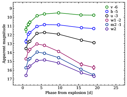
Figure 7: Swift UVOT light curves of SN 2017ahn. Magnitudes were calibrated to the Vega photometric system and have not been corrected for extinction.

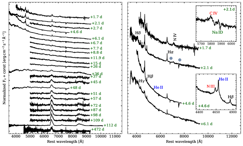
Figure 8: Left: Optical spectra of SN 2017ahn. Spectra were corrected for the total reddening along the line of sight. Right: Early spectroscopic evolution of SN 2017ahn. The spectrum at $+1.7\,\rm{d}$ is re-binned to a third of its original resolution to facilitate the visualization of the high-ionization features (see the main text). The most prominent features are identified. $\oplus$ symbols mark the position of the main telluric absorption features. Insets show zoom-in regions around Na ID (upper inset, including C IV $\lambda 5801$) at $+2.1\,\rm{d}$ and He II $\lambda 4686$ (bottom inset, including N III) at $+4.6\,\rm{d}$. Spectra used to create this figure are available as Data behind the Figure.

An upper limit in the X-ray counts was determined using aperture photometry through the HEAsoft packages (xselect; Blackburn 1995 and xspec; Arnaud 1996). The background was selected as a region outside the host galaxy with no known X-ray sources within, and measured fluxes were converted from counts per second to luminosities using PIMMS (Mukai, 1993). No significant detections were found over an 18″aperture integrating over all available SWIFT/XRT epochs. This resulted in a limiting count rate of $0.904\times 10^{-3}\,\rm{counts}\,\rm{s^{-1}}$, which, assuming a power-law model with a photon index of two and a Galactic absorption of $5.89\times 10^{20}\,\rm{cm^{-2}}$ (Kalberla et al., 2005), corresponds to an unabsorbed flux of $3.25\times 10^{-14}\,\rm{erg}\,\rm{cm^{-2}}\,\rm{s^{-1}}$ ($0.3-10\,\rm{keV}$) and a luminosity of $6.63\times 10^{39}\,\rm{erg}\,\rm{s^{-1}}$ at $33\,\rm{Mpc}$.

3.2 Optical spectra

Optical spectroscopy of SN 2017ahn was triggered soon after its discovery, with the first spectrum taken $+1.7\,\rm{d}$ after explosion (although an earlier NIR spectrum was obtained at $+1.4\,\rm{d}$, see Section 3.3). Final spectra are shown in Figure 8, while facilities used and reduction steps are described in Appendix B.

Early spectra show a very blue continuum with prominent narrow lines in emission, along with strong Na ID lines at the redshift of the host galaxy. The Na ID features are usually related to a non-negligible reddening along the line of sight of the transient (see, e.g., Poznanski et al., 2012), and their EWs ($0.53$ and 0.33 Å for D2 and D1, respectively), suggest a moderately extinguished environment for SN 2017ahn (see Section 2). At $+1.7\,\rm{d}$ and $+2.1\,\rm{d}$, the spectra show a number of narrow Balmer emission lines (H$\alpha$ to H$\delta$), along with He II $\lambda 5411$, C IV $\lambda 5801$, N III and N IV features. C IV and N IV features rapidly fade below the detection limit and are already not visible at $+4.6\,\rm{d}$, when, on the other hand, He II $\lambda 5411$ clearly emerges from the spectral continuum. High ionization features (i.e., N III,IV, C IV and He II) become progressively fainter with time, although the signal–to–noise (S/N) ratios and resolutions of our spectra do not allow us to rule out the presence of these lines at later phases. At $+6.1\,\rm{d}$ we also notice the appearance of a narrow He I $\lambda 5875$ feature, not visible at later epochs.

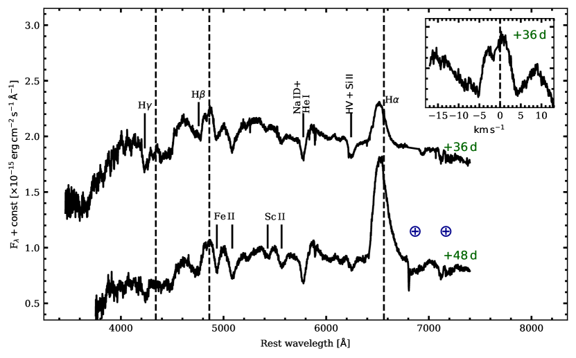
Figure 9: Identification of the main spectral features at $+36$ and $+48\,\rm{d}$. Dashed lines correspond to the rest wavelengths of the main Balmer lines, revealing the blue-shift of the emission peaks typical of SNe II (Anderson et al., 2014). $\oplus$ symbols mark the position of the residual telluric absorption features. A possible hydrogen high velocity (HV) feature is also labelled (see the discussion in the main text). In the inset, a zoom-in of the H$\beta$ region in the velocity space, showing the complex structure of the spectral region, with possible multiple absorption features centered at $\simeq-5000$ and $\simeq-10000$ km s^-1 with respect to H$\beta$ rest wavelength.

The total integrated luminosity (after removing the contribution of the spectral continuum and assuming the reddening reported in Section 2) of the N III+He II feature shows an initial increase from $\simeq 1.4\times 10^{40}$ erg s^-1 to $1.6\times 10^{40}$ erg s^-1 during the first $+4.6\,\rm{d}$, suggesting an increase in the production of ionizing photons in the underlying regions. We note the same evolution in the integrated luminosity of H$\alpha$, showing an increase of $\Delta L\simeq 1.2\times 10^{38}$ erg s^-1 over the same period, with a H$\alpha$/H$\beta$ ratio evolving from $\simeq 0.4$ (at $+2.1\,\rm{d}$) to $\simeq 1.9$ (at $+4.6\,\rm{d}$). At $+6.1\,\rm{d}$ the spectral shape shows the first significant signatures of evolution, with a drastic decrease in the integrated luminosity of the N III+He II feature ($\simeq 6.4\times 10^{39}$ erg s^-1) and the Balmer emission lines (e.g., $L_{\rm{H\alpha}}\simeq 1.6\times 10^{39}$ erg s^-1, with a H$\alpha$/H$\beta$ ratio of $\simeq 1.7$). We also note the appearance of broad and boxy absorption profiles in the blue part of the Balmer lines, with blue wings extending up to $\simeq 10^{4}$ km s^-1, corresponding to expansion velocities of the H-rich shell of $\simeq 6500$ km s^-1 (as derived from the minimum inferred through a Gaussian fit to the line profile).

At later epochs, spectra show a further drastic change, with broad P Cygni profiles becoming progressively stronger (see Figure 9) and the spectral evolution resembling that of a typical Type II SN (see, e.g., Gutiérrez et al., 2017). At $+36\,\rm{d}$ we clearly see broad Fe II (multiplet 42) and He I/Na ID features. At the same phases we also identify Sc II and a first hint of the presence of the NIR Ca II triplet, which remains relatively faint throughout the rest of the spectroscopic evolution (see Figure 8), except for the $+112\,\rm{d}$ spectrum, characterized by a significantly higher S/N at the corresponding wavelengths. At $+112\,\rm{d}$, we also notice broad forbidden [O I] $\lambda\lambda 6300,6364$ and [Ca II] lines, typical of the nebular phases of Type II SNe, with an integrated luminosity of $\simeq 6.4\times 10^{38}$ erg s^-1 and $\simeq 2.3\times 10^{39}$ erg s^-1, respectively. At $+472\,\rm{d}$ the spectrum only shows a boxy, flat-topped H$\alpha$ emission (see Figure 10), although the S/N does not allow us to rule out the presence of other nebular features at this epoch. Similarly, the S/N of the spectra at $+51\,\rm{d}\leq t\leq+109\,\rm{d}$ does not allow us to rule out the appearance of a boxy profile at earlier phases, which would reveal the presence of different CSM layers.

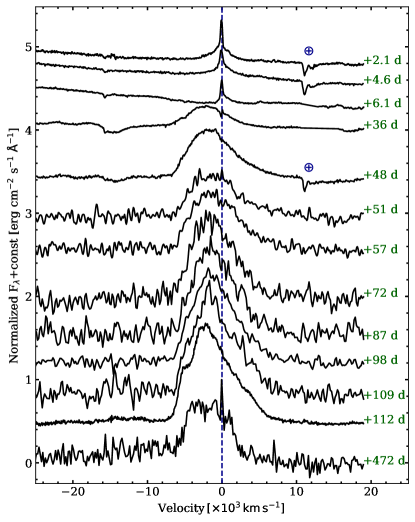
Figure 10: Evolution of the profile of H$\alpha$ over the first $472\,\rm{d}$ of evolution of SN 2017ahn. Velocities were computed with respect to H$\alpha$ rest wavelength. $\oplus$ symbols mark the position of the main telluric absorption features, if visible. The spectrum at $+472\,\rm{d}$ has been degraded to 1/3 of its resolution to facilitate the comparison.

Measuring the positions of the absorption minima at $+36\,\rm{d}$, we infer expansion velocities of $\simeq 5000$ km s^-1 from both H$\beta$ and Fe II $\lambda 5169$, the latter usually considered a good proxy of the SN photospheric velocity (see, e.g., Dessart & Hillier, 2005; Takáts & Vinkó, 2012), although the complex structure of the spectral region around H$\beta$ might suggest higher expansion velocities for the H-rich shell; see the inset in Figure 9. We infer similar values from Sc II lines, while we do not notice a significant evolution in the expansion velocities inferred at $+36$ and $+48\,\rm{d}$.

We obtained a rough estimate of the temperature evolution of the pseudo-photosphere fitting a black-body (BB) function to the spectral continuum, resulting in $T=10000\pm 900\,\rm{K}$ in both the $+1.7$ and $+2.1\,\rm{d}$ spectra. At $+4.6\,\rm{d}$ we note a drastic increase in the temperature ($\simeq 31000\pm 5000\,\rm{K}$), also reflected by the evolution of the spectral energy distribution (SED) inferred from photometry at the same epoch (see Section 4), followed by a progressive decrease to $\sim 5600\pm 600\,\rm{K}$ during the following $\sim 30\,\rm{d}$. Although prominent Balmer lines (in particular H$\alpha$ and H$\beta$) and high-ionization features can largely affect the shape of the pseudo-continuum, we do not see a significant improvement in the fit, and we do not get different temperatures excluding regions dominated by narrow emission lines. On the other hand, the high temperatures inferred during the first $6.1\,\rm{d}$ suggest a SED peaking at bluer wavelengths, not covered by the optical spectra, which in turn can significantly affect the proper determination of the temperature of the pseudo-continuum.

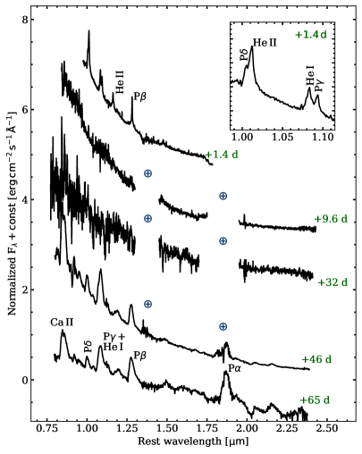
Figure 11: NIR spectra of SN 2017ahn. Spectra were corrected for the Galactic and host extinction and wavelengths have been corrected for redshift as inferred from the positions of the narrow Na ID galactic features. $\oplus$ symbols mark the positions of the most important telluric absorption features. The $+65\,\rm{d}$ spectrum is shown in logarithmic scale in order to facilitate the comparison with earlier spectra. Spectra at $+9.6\,\rm{d}$ and $+32\,\rm{d}$ have been re-binned to $1/3$ of their original resolutions to increase their S/N ratios. The inset shows a line identification in the blue part of the spectrum at $+1.4\,\rm{d}$. Spectra used to create this figure are available as Data behind the Figure.

Balmer lines are visible throughout the spectroscopic evolution of SN 2017ahn. Up to $+4.6\,\rm{d}$, the most prominent H lines (i.e., H$\alpha$ and H$\beta$) are purely in emission, with a slightly blue-shifted peak ($V_{shift}\simeq 70$ km s^-1, probably due to a ‘macroscopic’ velocity $V_{bulk}$ of the recombining shell; see Fransson et al., 2014), characterized by narrow cores with a full–width–at–half–maximum (FWHM) of $\simeq 300$ km s^-1, and broader wings extending up to full–width–at–zero–intensity (FWZI) of $\simeq 4000$ km s^-1. Similar velocities are also inferred from the profile of H$\beta$. While the overall profile might be contaminated by host lines (such as [N II] $\lambda\lambda 6548,6583$), we note that the H$\alpha$ is not well reproduced using a single Gaussian or Lorentzian profile. This might either suggest the presence of recombining shells moving at different velocities, or a broadening due to electron scattering in a dense ionized medium (see Section 4). At $+6.1\,\rm{d}$, the flux of the narrow Balmer lines decrease significantly (see above) and broad boxy absorption features appear in the blue part of H$\alpha$ and H$\beta$. Interestingly, we infer different expansion velocities from the absorption minima of H$\alpha$ and H$\beta$  ($V_{\rm{H}\alpha}=6500$ km s^-1 vs $V_{\rm{H}\beta}=1400$ km s^-1), suggesting an intrinsic difference in the expansion velocities of the absorbing shells. At $t\geq+36\,\rm{d}$, the H$\alpha$ region ($6100-6700$ Å) is dominated by a broad, blue-shifted and boxy emission and a broad boxy absorption component, with expansion velocities extending from $\simeq 1.2\times 10^{4}$ to $\simeq 1.8\times 10^{4}$ km s^-1 with respect to H$\alpha$ rest wavelength, becoming progressively fainter and disappearing at $t\gtrsim 51\,\rm{d}$. This can alternatively be identified as Si II $\lambda 6355$, which would result in expansion velocities comparable to those derived from Fe II $\lambda 5169$ (see Section 4). This interpretation is also supported by the overall shape of the emission component, symmetric with respect to its centroid and well reproduced using a single Gaussian profile with a FWHM of $\simeq 5800$ km s^-1. At the same epoch, H$\alpha$ also shows a sharp P Cygni profile with a narrow emission component roughly peaking at the line rest-wavelength, with an absorption component extending up to $3\times 10^{3}$ km s^-1, reminiscent of narrow features observed in sufficiently high-resolution spectra of Type IIn SNe (see, e.g. Fransson et al., 2014; Tartaglia et al., 2020). A more in-depth analysis also reveals an alternative decomposition, with H$\alpha$ being the sum of a narrower component on top of a broader, flat-topped profile, also resulting in the presence of a blue ‘shoulder’, similar to that observed in SN 2013L (see, e.g., Figures 22 and 24 in Taddia et al., 2020) and other similar interacting transients. This is also confirmed by the H$\alpha$ profile at $+472\,\rm{d}$ (see Figure 10).

3.3 Near infrared spectra

NIR spectroscopy of SN 2017ahn was triggered soon after discovery and resulted in a very early observation performed only $1.4\,\rm{d}$ after the estimated explosion epoch. To our knowledge, this is the earliest NIR spectrum of a Type II SN ever obtained. The complete NIR spectroscopic follow-up campaign spanned a period of $\sim 65\,\rm{d}$ and spectra are shown in Figure 11, while reduction steps and information about the facilities used are described in Appendix B.

At $+1.4\,\rm{d}$, the spectrum shows a blue continuum with prominent narrow Paschen ($\rm{Pa}\beta$ to $\rm{Pa}\delta$) lines, He I ($\lambda 10830$) and He II ($\lambda 10124$ and $\lambda 11626$) lines in emission, analogous to the flash features seen in the early optical spectra. At later times we note a spectroscopic evolution similar to that observed in the optical spectra, with a blue, almost featureless continuum at both $+9.6$ and $+32\,\rm{d}$, with a progressive metamorphosis towards spectroscopic features typical of photospheric phases of Type II SNe. At $+46\,\rm{d}$, roughly corresponding to the end-point of the plateau phase (see Section 3.1), we note broader Paschen lines ($\rm{Pa}\alpha$ to $\rm{Pa}\delta$), along with $\rm{Br}\beta$ and He I $\lambda 10830$ features, becoming stronger at $+65\,\rm{d}$ (see Figure 11). At this epoch, He I clearly shows a P Cygni profile, with an absorption component extending up to $13400$ km s^-1, possibly consisting in a high-velocity (HV) component centered at $-8650$ km s^-1, with a redder one centered at $-6300$ km s^-1 with respect to He I rest wavelength. We note a similar structure also at $+65\,\rm{d}$, suggesting that this feature is real, although we cannot rule out the contribution of other lines such as P$\gamma$ and Sr II. If real, along with the measured EW ($\simeq 10$ Å at $+46\,\rm{d}$), this would suggest a “weak” classification for SN 2017ahn when compared to the sample presented in Davis et al. (2019). On the other hand, given the lack of the blue “notch” in the He I emission component, attributed to P$\gamma$+Sr II and typically observed in weak SNe, we favor the P$\gamma$+Sr II identification for the blue feature, which in turn would suggest a “strong” classification for SN 2017ahn. This would also confirm the claim that fast declining Type II SNe belong to the strong subclass (see Davis et al., 2019).

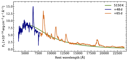
Figure 12: Combined optical+NIR spectra of SN 2017ahn at $+48\,\rm{d}$ and $+65\,\rm{d}$. The spectral continuum is fairly well reproduced by a single BB (although affected by significant line-blanketing at $\lambda\lesssim 5000$ Å), ruling out the presence of a colder component at least until $+65\,\rm{d}$

Isolated narrow lines at $+1.4\,\rm{d}$ (i.e., $\rm{Pa}\beta$ and He II $\lambda 10124$) are fairly well reproduced by a single Lorentzian profile, suggesting that the lack of broader electron scattering wings is most likely due to the lower resolution compared to the $+2.1\,\rm{d}$ and $+4.6\,\rm{d}$ optical spectra (see Figure 8 and the description of optical spectra in Section 3.2). By $t=+9.6\,\rm{d}$, the $\rm{Pa}\beta$ integrated luminosity shows a decrease of $\Delta L=3.3\times 10^{38}$ erg s^-1 and also high-ionization He II lines fade below the level of the spectral continuum. At $+46\,\rm{d}$ and $+65\,\rm{d}$, Paschen lines show a slightly asymmetric profile, although still reasonably well reproduced by Gaussian profiles with FWHM of $\simeq 6500$ km s^-1.

Fitting a BB to the spectral continuum we find an evolution similar to that observed in the optical spectra, although with slightly lower temperatures. Given the lack of NIR photometric data after peak and the similar spectroscopic evolution to that observed in SN 1998S, we investigate the possible presence of an IR excess by shifting the blue part of the NIR spectra at $t>+9.6\,\rm{d}$ (i.e. the epochs missing a proper absolute flux calibration against photometry) in order to match the red parts of the optical spectra obtained at similar phases. In addition, we also compute synthetic $z,J,H,K$ magnitudes from the derived spectra, in order to have an estimate of the NIR part of the SED at these epochs (see Section 4). In Figure 12 we show the resulting optical+NIR spectrum obtained combining the $+48\,\rm{d}$ optical spectrum with the $+65\,\rm{d}$ NIR one, clearly showing no evidences of a colder component, at least until $+65\,\rm{d}$.

4 Analysis and discussion

In the following, we will derive and discuss the main physical quantities obtained through simple modeling of the main observables described in the previous sections. In Sections 4.3 and 4.4 we will also discuss the results of our numerical modeling of the early evolution of SN 2017ahn, and compare our results to those predicted by hydrodynamical models available in the literature.

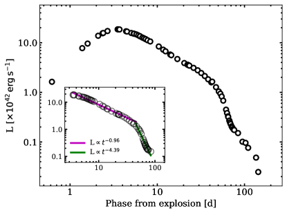
Figure 13: Evolution of the pseudo-bolometric luminosity of SN 2017ahn in logarithmic scale. In the inset, a zoom-in of the region between $+3.5\,\rm{d}$ and $+86\,\rm{d}$, showing the ‘broken power-law’ typical of interacting transients, with an initial evolution described by $L(t)\propto t^{-0.96}$ followed by a steeper decline described by $L(t)\propto t^{-4.39}$ with the break occurring at $t\simeq+45\,\rm{d}$.

4.1 Evolution of the bolometric luminosity

The evolution of the bolometric luminosity was estimated following the prescriptions of Tartaglia et al. (2020), including the contribution to the SED of the early UV bands at $t\lesssim 20\,\rm{d}$ and extending the $z,J,H,K$ light curves up to $+65\,\rm{d}$ using synthetic magnitudes obtained from calibrated NIR spectra (see Section 3.3). The derived SEDs at each epoch were integrated using BBs without introducing any ‘suppression’ factor at wavelengths bluer than $\sim 3000$ Å (see, e.g., the discussion in Nicholl et al., 2017). This approach is based on a compromise between absorptions due to line blanketing (see, e.g., Pastorello et al., 2010; Chomiuk et al., 2011) and the UV flux excess predicted by synthetic spectra of Type IIn SNe (see, e.g., Figure 13 and the discussion in Dessart et al., 2015). Based on these considerations, the resulting evolution, shown in Figure 13, should still be considered as a ‘pseudo-bolometric’ light curve, possibly underestimating the actual luminosity of SN 2017ahn, in particular at early phases.

The bolometric light curve shows a fast rise lasting $\simeq 3.7\,\rm{d}$ with a peak luminosity of $\simeq 1.9\times 10^{43}$ erg s^-1 rapidly declining to $2.5\times 10^{40}$ erg s^-1 at $\sim+144\,\rm{d}$. The corresponding total radiated energy within the first $\sim 144\,\rm{d}$ is $\simeq 2.3\times 10^{49}\,\rm{erg}$. At $+3.5\,\rm{d}\leq t\leq+86\,\rm{d}$ the luminosity evolution is well reproduced by a broken power-law, a behavior typically observed in Type IIn SNe and other interacting transients (see, e.g., Fransson et al., 2014; Ofek et al., 2014; Tartaglia et al., 2020). We find that the bolometric light curve is well reproduced by $L(t)=7.47\times 10^{43}\,t^{-0.96}$ erg s^-1 up to $\simeq+40\,\rm{d}$, followed by a much steeper decline described by $L(t)=3.1\times 10^{49}\,t^{-4.39}$ erg s^-1 up to $\sim+86\,\rm{d}$.

The late-time (i.e., during the post-plateau phases) bolometric light curve can be used to infer the mass of the radioactive ${}^{56}\rm{Ni}$ expelled by the SN explosion. During the nebular phase, the bolometric light curves of SNe settle onto a “radioactive” tail, where the energy output is dominated by the ${{}^{56}\rm{Co}}\rightarrow{{}^{56}\rm{Fe}}$ decay. Assuming full $\gamma$-ray trapping (and hence a decline of $\simeq 1\,\rm{mag}\,100\,\rm{d^{-1}}$) within the opaque SN ejecta, it is therefore possible to get an estimate of the ejected ${}^{56}\rm{Ni}$ mass through direct comparison of the late-time luminosity with that of SN 1987A at similar phases, through the relation:

$$M({{}^{56}\mathrm{Ni}})=0.075M_{\odot}\times\frac{L_{SN}(t)}{L_{87A}(t)}$$ (1)

(see, e.g., Spiro et al., 2014, and references therein).

Figure 14: Fit of the modified radioactive decay model to the late-time bolometric light curve of SN 2017ahn. The full $\gamma$-ray trapping model is shown as a comparison.

Figure 15: Posterior probability distributions and correlations between temperature (T1) and total luminosity (L1) at $+1\,\rm{d}$, the epoch at which the envelope becomes transparent ($t_{tr}$), and discovery epoch ($\Delta t_{0}$) following the prescriptions of Hosseinzadeh et al. (2018). Shock cooling models are not able to reproduce the early light curves of SN 2017ahn.

On the other hand, the late-time evolution of SN 2017ahn (see Figure 14) shows a much steeper decline if compared to the one expected from the radioactive ${}^{56}\rm{Co}$ decay. This is probably due to a non-complete trapping of the $\gamma$-rays produced in the radioactive decay. A similar evolution was also observed in the Type II-L SN 2014G, also showing high ionization features in early spectra, and attributed to a non-complete trapping of the $\gamma$-rays produced in the ${}^{56}\rm{Co}$ decay (Terreran et al., 2016). Non-complete trapping has been discussed by Clocchiatti & Wheeler (1997), who found a simple relation to describe the late-time photometric evolution for a sample of stripped envelope SNe:

$$L(t)=L_{0}(t)\times\left[1-e^{-(T_{0}/t)^{2}}\right]$$ (2)

with $T_{0}$ the full-trapping characteristic time-scale defined as:

$$T_{0}=\left(C\kappa_{\gamma}\frac{M^{2}_{ej}}{E_{k}}\right)^{1/2},$$ (3)

where $M_{ej}$, $E_{k}$ and $k_{\gamma}$ are the total ejected mass, kinetic energy and the $\gamma$-ray opacity and $C$ a constant given by $C=(\eta-3)^{2}[8\pi(\eta-1)(\eta-5)]$ for a density profile of the radioactive matter $\rho(r,t)\propto r^{-\eta}(t)$. The theoretical luminosity due to fully trapped ${}^{56}\rm{Co}$ energy deposition is given by (see, e.g., Jerkstrand et al., 2012, and references therein):

$$L_{0}(t)=9.92\times 10^{41}\frac{M_{{}^{56}\mathrm{Ni}}}{0.07\,M_{\odot}}\left(e^{-t/111.4}-e^{-7/8.8}\right)\,\mathrm{erg}\,\mathrm{s^{-1}}$$ (4)

where $M_{{}^{56}\rm{Ni}}$ is the Ni mass expelled by the SN explosion. This model simply assumes spherical symmetry and homologous expansion of shells with the entire radioactive matter located at the center of the explosion.

Including Equation 4 into Equation 2, we then fit the late-time bolometric light curve of SN 2017ahn to get a rough estimate of the ejected ${}^{56}\rm{Ni}$ mass and the full-trap characteristic time-scale, performing $10^{4}$ Monte Carlo simulations, randomly shifting the luminosities within their errors. The resulting fit, giving $M_{{}^{56}\rm{Ni}}=0.041\pm 0.006$ M_☉ and $T_{0}=72\pm 7\,\rm{d}$ is shown in Figure 14. This is consistent with the median value found by Anderson (2019) for a sample of Type II SNe (0.032 M_☉).

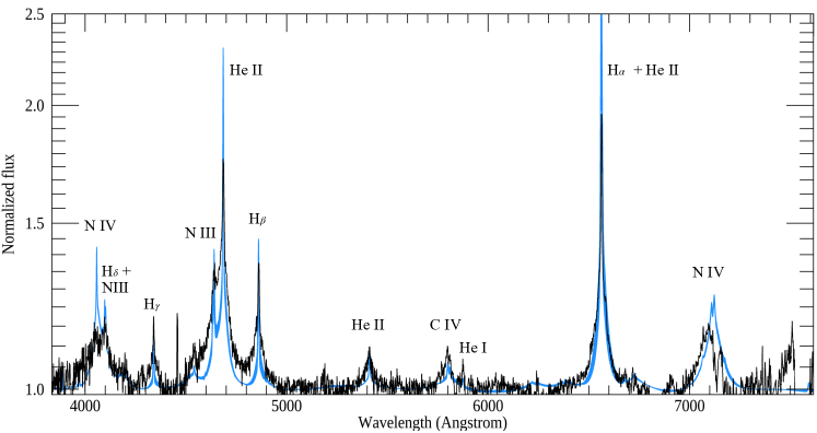
Figure 16: Best-fitting CMFGEN models (blue region) compared to the $+2.1$ d optical spectrum of SN 2017ahn. See Section 4.3 for our modeling technique and allowed range of parameters.

4.2 Shock cooling modeling of the early light curves

Theoretical SN models predict a short (seconds to hours) flash of X-ray/UV radiation to be emitted once the radiation mediated shock breaks through the stellar envelope, followed by UV/optical emission from the rapidly expanding and cooling layers. The analysis of the early post-break cooling phases can be used to infer crucial SN progenitor parameters, including its radius and surface chemical composition (see, e.g., Waxman & Katz, 2017). In particular, the photospheric temperature and luminosity evolution during the early SN evolution can be described analytically as a function of the shock velocity, the opacity of the expanding medium and the mass and radius of the progenitor star (see, e.g., Rabinak & Waxman, 2011).

We model the early photometric evolution of SN 2017ahn in the context of early SN light curves being dominated by shock cooling radiation escaping from the rapidly expanding progenitor envelope (see Sapir & Waxman, 2017) using the same approach adopted by Hosseinzadeh et al. (2018), fitting multi-band light curves assuming $n=3/2$ (polytropic index for a typical RSG envelope) with a Markov Chain Monte Carlo (MCMC) routine with flat priors for all parameters, 100 walkers and 500 steps (see Hosseinzadeh, 2020). The resulting fit (Figure 15) shows that the model fails to reproduce the early photometric evolution of SN 2017ahn, which seems to show faster rise times in the UV bands and brighter peaks, in particular in the bluer optical bands.

A plausible explanation must account for an extra source of energy, which, in turn, would affect the accuracy and validity of the Sapir & Waxman (2017) model. A similar explanation was given by Hosseinzadeh et al. (2018) to explain the fast early evolution of SN 2016bkv. Interaction with high-velocity SN ejecta and a dense, pre-existing medium, which is typically considered to power the light curves of narrow-lined transients (e.g., SNe IIn; Schlegel 1990 and Ibn; Pastorello et al. 2016), can affect the overall shape of the light curve (both at early and late phases) and would require a different physical interpretation of the early SN phases. In stellar explosions occurring within a dense CSM, in fact, the SN shock is expected to break through the dense CSM surrounding the progenitor star rather than the stellar envelope, extending and diluting the SN radiation, with early light curves being dominated by photon diffusion rather than shock-cooling emission.

Although narrow lines are generally considered an indirect proof of ongoing interaction between expanding SN ejecta and a dense pre-existing CSM, high-ionization features (C IV, N III and N IV) are typically observed only at the very early phases (hours to a few days after explosion) and are believed to arise from the recombining CSM ionized by the shock breakout flash, rather than by photons emitted in shocked regions. On the other hand, in SN 2017ahn, such features disappear $\simeq 6\,\rm{d}$ after explosion, suggesting a simple scenario where the recombining CSM is progressively swept up by the rapidly expanding ejecta. Under specific conditions, an efficient conversion of kinetic energy into radiation would therefore be able to provide the required energy input to explain the early evolution of SN 2017ahn. This is also in agreement with the results obtained by Morozova et al. (2017, see also ) modeling the light curves of fast-declining Type II SNe, suggesting red supergiants surrounded by a dense CSM as viable progenitors and that the presence of such dense medium might be common among H-rich CC SNe. Although the pseudo bolometric light curve of SN 2017ahn does not show the sudden drop at $t\simeq+25\,\rm{d}$ predicted by the models of Moriya et al. (2011, corresponding to the dense shell becoming optically thin and the photosphere receding into the SN ejecta, see, e.g., their Figure 4), its overall shape is similar to their $10^{-3}$ M_☉ yr^-1 model (see Sections 4.3 and 4.4).

Interaction would also explain narrow H$\alpha$ components with sharp P Cygni profiles at later times, observed up to $+36\,\rm{d}$ and the prominent boxy profile observed in the H$\alpha$ profile at $t>+36\,\rm{d}$ (Figure 10), showing a progressively asymmetric profile with a characteristic blue-shifted ($V_{shift}\simeq 5000$ km s^-1) “shoulder”. Similar features are common among Type II SNe showing linearly declining light curves (see, e.g., the cases of SNe 1999ga Pastorello et al. 2009 and 2017ivv Gutiérrez et al. 2020 and the objects in the sample of Faran et al. 2014) as well as in a few Type IIn SNe at sufficiently late times (see, e.g., the cases of SNe 2005ip Stritzinger et al. 2012; Smith et al. 2017 and 2013L Taddia et al. 2020) and are typically considered evidence of emission from a shocked thick shell of gas (see, e.g., Jerkstrand, 2017). Ongoing interaction of SN ejecta with a dense CSM at $t\gtrsim+6\,\rm{d}$ (i.e., when high-ionization features seem to disappear) is also consistent with the radio non-detection of SN 2017ahn at 5.5 and $9\,\rm{GHz}$ (Ryder et al., 2017), suggesting efficient synchrotron self absorptions by free electrons in a dense medium at $+21\,\rm{d}$.

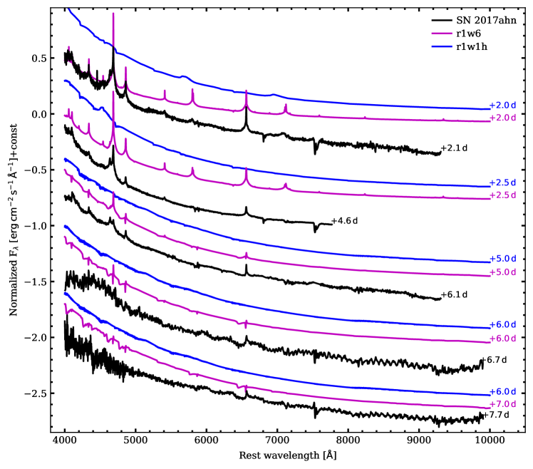
Figure 17: Comparison of the early ($t\lesssim 8\,\rm{d}$) spectra of SN 2017ahn, corrected for the total reddening reported in Section 2, with a selection of Dessart et al. (2017) models. Model r1w1h reproduces well the shape of the continuum at all phases, although it does not show emission features observed in the early spectra of SN 2017ahn. Model r1w6 is able to reproduce both the spectral continuum and most of the emission lines at $t>+2.5\,\rm{d}$, while at $+2\,\rm{d}$ the overall spectral features are not reproduced well by none of the models presented in Dessart et al. (2017). The choice of these models is based on their similar evolutions with respect to SN 2017ahn, including the presence of high-ionization features (e.g., Ne III, He II, C III,IV) at early phases, the shape of the continuum and the timescale at which the spectra evolve (e.g., all other models have a much faster evolution, with high-ionization features disappearing a few hours after the shock-breakout; see Figures C.1-C.7 in Dessart et al. 2017). These both correspond to a progenitor radius $R_{\star}=501$ R_☉, with mass-loss rates $10^{-6}$ (r1w1h) and $10^{-2}\,\rm{M_{\odot}}\,\rm{yr^{-1}}$ (r1w6, with $\dot{M}=10^{-6}\,\rm{M_{\odot}}\,\rm{yr^{-1}}$ beyond $5\times 10^{14}\,\rm{cm}$, see the main text and Dessart et al. (2017) for more details).

4.3 CMFGEN models of the early interaction

To investigate the properties of SN 2017ahn at early times, we compute numerical models using the radiative transfer code CMFGEN (Hillier & Miller, 1998a) with the implementation of Groh (2014). In our models, photons diffuse out through the extended material around the progenitor. Although we do not need to assume a source of energy, the photons are thought to be produced by the interaction between the SN ejecta and the progenitor wind. The wind heats up and emits continuum and line photons according to its temperature and density structure. Our main assumptions are of a spherical and stationary wind, radiative equilibrium to compute the temperature structure, non-local thermodynamic equilibrium, and time-independent radiative transfer. The models take as input the luminosity of the event $L_{\rm SN}$, the progenitor mass-loss rate $\dot{M}$, wind terminal velocity $\upsilon_{\infty}$ and surface abundances, and the location of the inner boundary $R_{in}$, which depends on the ejecta dynamics and time after explosion. Since the progenitor wind is dense, the photosphere is extended and we quote two flux temperatures, $T_{\star}$ at the inner boundary (Rosseland optical depth of $\tau\simeq 10.0$), and $T_{\rm eff}$ at $\tau=2/3$. We refer the reader to Boian & Groh (2018), Boian & Groh (2019) and Boian & Groh (2020) for further details.

We use the models presented in Boian & Groh (2020) as a starting point. These model grids were computed at 1.0, 1.8, and $3.8\,\rm{d}$ after explosion, exploring a wide range of parameters: $1.9\times 10^{8}\leq L\leq 2.5\times 10^{10}$ L_☉, $5\times 10^{-4}\leq\dot{M}\leq 10^{-2}\,\rm{M_{\odot}}\,\rm{yr^{-1}}$, three values of chemical abundances (solar, He-rich and CNO-processed) and fixed wind terminal velocities and ejecta expansion velocities of $\upsilon_{\infty}=1.5\times 10^{2}$ km s^-1 and $v_{ej}=10^{4}$ km s^-1, respectively. Once we find the best fit models among the Boian & Groh (2020) grid, we compute 30 additional models in this region of parameter space to obtain the properties of SN 2017ahn at $+2.1\,\rm{d}$, corresponding to our highest S/N optical spectrum around that epoch. Figure 16 shows our best fitting models compared with the observed spectrum.

We find that our CMFGEN models quantitatively reproduce the spectral morphology of SN 2017ahn at $+2.1\,\rm{d}$, with strong He II, H I, N III, and N IV features. Our models indicate $L=5.0-7.2\times 10^{9}$ L_☉, $\dot{M}=2.7-4.0\times 10^{-3}$ M_☉ yr^-1 (for $\upsilon_{\infty}=150$ km s^-1), $R_{in}=2.17\times 10^{13}\,\rm{cm}$, $T_{\star}=26600-28900\,\rm{K}$, surface mass fractions $C_{\rm sur}=5.6\times 10^{-5}$, $N_{\rm sur}=8.2\times 10^{-3}$, and $O_{\rm sur}=1.3\times 10^{-4}$, with an estimated 3-$\sigma$ error of 50% and a He surface mass fraction of $Y\simeq 0.35-0.50$, suggesting some He enhancement, consistent with the scenario that the progenitor lost a significant fraction of its H envelope before exploding. Fitting the observed SED implies a total color excess of $E(B-V)=0.06\pm 0.01\,\rm{mag}$ and $R_{V}=3.1$, which, although in line with the extinction values found for a large sample of interacting SN (Boian & Groh, 2020), is in contrast with the reddening derived from both the optical spectra (clearly showing strong Na ID features at all times; see Section 3.2) and the spectral analysis of the local environment (Section 2).

Our results show that the progenitor had CNO-processed surface abundances, with enhanced N and depleted C and O. The Geneva stellar evolution models suggest that this would be expected from a massive ($\sim 15-25$ M_☉) RSG, a YHG or a BSG/LBV star (Groh et al., 2013). However, these models make strong assumptions about rotational mixing and mass loss, which have a key impact on the final CNO surface abundances (Meynet et al., 2013, 2015). In addition, a significant fraction of massive stars evolve in binary systems (Sana et al., 2012), with important consequences for the final mass and surface abundances. Finally, the final mass of red supergiants could be much larger than previously thought (Farrell et al., 2020a, b). For all these reasons, it is challenging to map final surface abundances to progenitor initial or final masses (see also the discussion in Boian & Groh, 2020).

We remark that the above quantities should be taken with caution given our model assumptions. In particular, an important role may also be played by asymmetries and/or particular geometrical configurations of the CSM, which were also believed to affect the evolution of the observables of SN 1998S (see Leonard et al., 2000) as well as CC SNe in general. We encourage further constraints on the CSM morphology of interacting SNe, which would allow these effects to be taken into account in future modeling of the early evolution of SN 2017ahn.

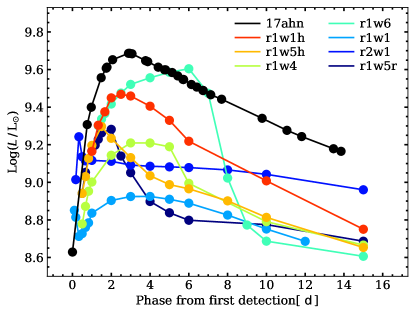
Figure 18: Comparison of the pseudo-bolometric light curve of SN 2017ahn with the uvoir models of Dessart et al. (2017). Model r1w1h, corresponding to a progenitor radius $R_{\star}=501$ R_☉ with a mass-loss rate $\dot{M}=10^{-6}\,\rm{M_{\odot}}\,\rm{yr^{-1}}$ and an atmospheric density scale height $H_{\rho}=0.1R_{\star}$ ($H_{\rho}=0.3R_{\star}$ down to $\rho=10^{-12}\,\rm{g}\,\rm{cm^{-3}}$; see the main text and Dessart et al. 2017 for details) reproduces well the shape of the light curve, although with a slightly fainter luminosity at all phases.

4.4 Comparison with existing hydrodynamic models

After investigating our own models, we now compare the early photometric and spectroscopic evolution of SN 2017ahn with existing hydrodynamical models available in the literature. Dessart et al. (2017) used 1-D radiation-hydrodynamics and 1-D non-local thermodynamical equilibrium (LTE) radiative transfer models to reproduce photometric and spectroscopic features of RSG stars exploding within moderately extended and massive winds, with $R_{w}\sim 10\,R_{\star}$ and a total mass $\lesssim 10$ M_☉. The resulting models were obtained using multi-group radiation-hydrodynamics simulations performed with heracles (González et al., 2007) and post-processed using the radiative transfer code cmfgen (Hillier & Miller, 1998b) with initial conditions described in Dessart et al. (2013, 2015). The result of a simple direct comparison of the observed early evolution of SN 2017ahn with their synthetic spectra is shown in Figure 17.

Although the evolution of the narrow spectral features is well matched by their r1w6 model, it fails to reproduce the shape of the blue spectral continuum, while the temperature of the pseudo photosphere is well matched by model r1w1h, which, on the other hand, is not able to reproduce the evolution of the high ionization features. These models both correspond to a RSG progenitor with $R_{\star}=501$ R_☉, a total ejected mass of 12.52 M_☉ with kinetic energy $E_{k}=1.35\times 10^{51}\,\rm{erg}$, colliding with a pre-existing confined wind extending from $10^{15}$ to $2\times 10^{16}\,\rm{cm}$, a total mass of 2.89 M_☉ (based on the mass of the CSM inferred by Fransson et al., 2014, for SN 2010jl) and an expansion velocity $u_{w}=10^{2}$ km s^-1. The model r1w6, in particular, corresponds to a mass-loss rate of $10^{-2}\,\rm{M_{\odot}}\,\rm{yr^{-1}}$ ($10^{-6}$ beyond $5\times 10^{14}\,\rm{cm}$), while r1w1h assumes $\dot{M}=10^{-6}\,\rm{M_{\odot}}\,\rm{yr^{-1}}$ with a density scale height $H_{\rho}=0.3R_{\star}$ followed by a power-law with index 12 above $10^{-12}\,\rm{g}\,\rm{cm^{-3}}$ ($H_{\rho}=0.1R_{\star}$; see Dessart et al., 2017). Model r1w1h also seems to reproduce well the shape of the pseudo-bolometric light curve of SN 2017ahn (see Figure 18, where we compare it with the $uvoir$ light curves from Dessart et al. 2017), although with lower luminosities at all phases.

The main difference of r1w1 and r1w1h is the adopted value for the mass-loss rate ($10^{-2}$ and $10^{-6}\,\rm{M_{\odot}}\,\rm{yr^{-1}}$ for the dense and weak-wind models r1w6 and r1w1h, respectively), suggesting an intermediate value for SN 2017ahn. This is in agreement with our modeling discussed in Section 4.3, which gives a mass-loss rate of $2.7-4.0\times 10^{-3}$ M_☉ yr^-1. This idea is also supported by the mass-loss rate inferred by Shivvers et al. (2015) from their modeling of the spectra of SN 1998S, resulting in $\dot{M}=6\times 10^{-3}\,\rm{M_{\odot}}\,\rm{yr^{-1}}$. On the other hand, we cannot rule out other explanations, as well as a combination of different parameters, including masses, velocities and kinetic energies of the expanding SN ejecta and the pre-existing CSM, or a different rate of conversion of kinetic energy into radiation. Dessart et al. (2015), for example, showed that a higher kinetic energy of the SN ejecta can give higher luminosities without affecting the overall shape of the light curve. Despite the limitations of our approach, the spectral and luminosity evolution predicted by models r1w6 and r1w1h are fairly in agreement with the observed evolution of SN 2017ahn, considering these models were not specifically constructed on its observables.

Based on their similar spectroscopic evolutions, we also compare the spectroscopic evolution of SN 2017ahn with the radiative transfer simulated spectra for SN 1998S presented in Dessart et al. (2016). Although the evolution of the narrow features seems to be slower (see Figure 19), Model A (see Figure 5 in Dessart et al., 2016) is able to reproduce well both the shape of the spectral continuum and the spectral features observed in SN 2017ahn, although it fails to reproduce the N III+He II feature observed at $\leq+6.1\,\rm{d}$. This model, similar to that proposed by Chugai et al. (2004) for the Type IIn SN 1994W, corresponds to a massive ($M_{ej}=10$ M_☉) and energetic $E_{k}=10^{51}\,\rm{erg}$ shell ramming into a 0.4 M_☉ dense CSM, produced by a stationary wind with a mass-loss rate of 0.1 M_☉ yr^-1 with an expansion velocity of $10^{2}$ km s^-1 (see also Appendix A of Dessart et al., 2016, for more details about the model). These parameters are in contradiction with those inferred from simple comparison with other pre-existing models (see above), highlighting the need of a more accurate modeling.

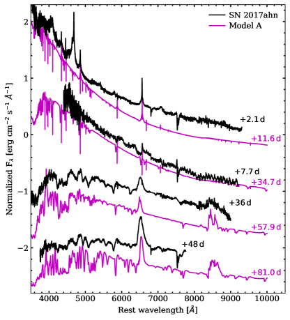
Figure 19: Comparison of the spectroscopic evolution of SN 2017ahn at selected epochs with “Model A” computed for SN 1998S in Dessart et al. (2016).

5 Summary and conclusions

In this paper, we discussed the photometric and spectroscopic properties of the Type II SN 2017ahn, discovered soon after explosion by the DLT40 survey in the nearby galaxy NGC 3318. Multi-wavelength follow-up campaigns, promptly activated after discovery, revealed a relatively fast early photometric evolution, showing peculiar fast rising light curves in UV bands, suggesting a very high initial temperature of the pseudo photosphere.

Like in SN 1998S, the early spectral evolution is characterized by the presence of prominent and narrow high-ionization features with narrow unresolved cores and broad wings. These are typical of electron scattering profiles observed in Type IIn SNe, and are expected to be common during the very early phases of the evolution of CC SNe. These features get progressively fainter and disappear roughly a week after explosion, suggesting the presence of a confined dense shell, progressively swept up by the expanding SN ejecta.

At later times, the evolution of SN 2017ahn resembles those typically observed in fast declining Type II SNe, with a short plateau-like phase lasting $\sim 50\,\rm{d}$, followed by a tail similar, although slightly steeper, to that predicted by the ${}^{56}\rm{Co}$ radioactive decay during the nebular phases of SNe. According to Faran et al. (2014), the rapid decline rates observed in objects like SN 2017ahn both during the plateau and the nebular phases are consistent with those expected by fast declining Type II SNe. Comparing the late evolution of the pseudo bolometric light curve of SN 2017ahn to that of SN 1987A, we estimate an ejected ${}^{56}\,\rm{Ni}$ mass of $0.041\pm 0.006$ M_☉, with a non-complete trapping of the $\gamma-$rays produced in the radioactive Co decay, although this measurement could be affected by ongoing ejecta-CSM interaction.

A non-negligible contribution of the interaction is also suggested by the evolution of the bolometric luminosity showing a broken power-law shape just before settling on the radioactive tail, while H$\alpha$ shows a late-time structured profile with a peculiar blue shoulder consistent with a boxy flat-topped emission component. In addition, the poor fit of the early light curves to shock-cooling models might also reveal a significant contribution of interaction to the total luminosity already at early times.

Numerical modeling of the early evolution of SN 2017ahn using the radiative transfer cmfgen (Hillier & Miller, 1998b) code suggests a massive ($15-25$ M_☉) progenitor for SN 2017ahn, with a initial radius of $\simeq 310$ R_☉ and a mass-loss rate $\dot{M}=2.7-4.0\times 10^{-3}\,\rm{M_{\odot}}\,\rm{yr^{-1}}$ (assuming $\upsilon_{\infty}=1.5\times 10^{2}$ km s^-1). A similar result was obtained through direct comparison with existing non-LTE radiative-transfer models obtained with the heracles (González et al., 2007) and cmfgen codes, suggesting a progenitor with a plausible mass-loss rate of $\simeq 3\times 10^{-3}\,\rm{M_{\odot}}\,\rm{yr^{-1}}$, although these models assume a less massive RSG progenitors (with an intial mass of $\simeq 14$ M_☉) and terminal velocity ($\upsilon_{\infty}=50$ km s^-1, see Dessart et al., 2013, 2017). Although both approaches can give models matching many features observed in SN 2017ahn, none of them is able to account for complex geometrical configurations, binarity of the progenitor system and their consequences on the final masses and surface abundances, or reproduce completely the early evolution of the observables, suggesting the need for continued modeling efforts. Nonetheless, the data and models support the idea that linearly declining Type II SNe arise from massive stars depleted of a significant fraction of their H-rich envelope in the pre-SN stage.

Appendix A Photometric data

PROMPT5 unfiltered DLT40 images were reduced as in Tartaglia et al. (2018), using our dedicated pipeline and calibrated to the $r$-band. Magnitudes are reported in Table 1.

Optical photometry of SN 2017ahn was obtained mostly using the facilities of the Las Cumbres Observatory network (Brown et al., 2013) within the Supernova Key Project. Additional optical and NIR photometry was obtained, as part of the GREAT survey (Chen et al., 2018), using the Gamma-Ray Burst Optical/Near-Infrared Detector (GROND; Greiner et al., 2008), a 7-channel imager, collecting multi-color photometry in $g^{\prime},r^{\prime},i^{\prime},z^{\prime}$ and $J,H,K_{\rm{S}}$ bands simultaneously, mounted at the $2.2\,\rm{m}$ MPG telescope at ESO La Silla Observatory in Chile. These frames were pre-reduced using the dedicated GROND pipeline (Krühler et al., 2008), including bias and flat-field corrections, image stacking and astrometric calibrations. Both optical and NIR magnitudes were obtained using the dedicated pipeline SNOoPY and are listed in Tables 2, 3 and 5.

Swift data were reduced using the pipeline of the Swift Optical Ultraviolet Supernova Archive (SOUSA; Brown et al., 2014), which is based on the method of Brown et al. (2009) using the zero points of Breeveld et al. (2011). The uncertainties account for differences in the measured brightness using a range of background regions with galaxy light similar to that of the SN. Magnitudes are reported in Table 4

Appendix B Spectroscopic data

Optical spectra of SN 2017ahn were obtained using the facilities listed in Table 6. Most of the spectra were obtained using the Faulkes Telescopes $2\,\rm{m}$ telescopes of the Las Cumbres Observatory network, located at the Haleakala Observatories (Faulkes Telescope North, Hawaii – U.S.; FTN) and the Siding Spring Observatory (Faulkes Telescope South, Australia; FTS) using the cross-dispersed, low resolution spectrographs FLOYDS and reduced using their dedicated pipeline (Valenti et al., 2014). Optical spectra were also obtained using the $10\,\rm{m}$ Southern African Large Telescope (SALT), located at the South African Astronomical Observatory (SAAO), Sutherland, South Africa, with the Robert Stobie Spectrograph (RSS) (reduced using the dedicate pipeline PySALT; Crawford et al., 2010) and the $4.1\,\rm{m}$ SOuthern Astrophysical Research telescope (SOAR) with the Goodman High Throughput Spectrograph (Clemens et al., 2004), located at the Cerro Tololo Inter-American Observatory, Cerro Pachón, Chile and reduced using a dedicated pipeline. One additional optical spectrum was obtained using the $10\,\rm{m}$ Keck I telescope located at the Mauna Kea Observatories (Hawaii, U.S.) using the Low Resolution Imaging Spectrometer (LRIS; Oke et al., 1995; Rockosi et al., 2010) and reduced using the automated pipeline lpipe (Perley, 2019). MUSE data reduction was performed using the ESO MUSE data reduction pipeline under the Reflex interface (Freudling et al., 2013), which includes bias subtraction, flat-fielding, wavelength and flux calibrations, background sky subtraction and atmospheric effects correction. The spectra were subsequently extracted from the reduced MUSE datacube for further analysis.

Near-infrared (NIR) spectra were taken with the FLAMINGOS-2 instrument (F2; Eikenberry et al., 2006) at Gemini South Observatory, SpeX instrument (Rayner et al., 2003) on the NASA Infrared Telescope Facility and the Folded-port InfraRed Echellette instrument (FIRE; Simcoe et al., 2013b) on the Magellan Baade telescope. The IRTF SpeX data was taken in cross-dispersed SXD mode with the 0.5 arcsec slit, yielding wavelength coverage from $\sim 0.7-2.4\,\rm{\mu m}$ and a $R\sim 1200$. The Magellan FIRE spectra were obtained in high throughput prism mode with a 0.6″ slit, giving continuous wavelength coverage from 0.8 to $2.5\,\rm{\mu m}$. For the Gemini South F2 spectra, we observed with the JH grism and 0.72″ slit in place, yielding a wavelength range of $1.0-1.8\,\rm{\mu m}$. All observations were taken with a standard ABBA pattern for sky subtraction, and an A0V star was observed adjacent to the science exposures for both telluric corrections and flux calibration. Data for both instruments was reduced in a standard way as described in Hsiao et al. (2019), and we refer the reader there for the details.

Table 1: DLT40 unfiltered light curves of SN 2017ahn. Magnitudes are calibrated to the $r$-band.

Date	JD	phase	$Open$(err)
		d	(mag)
20170205	2457789.74	-2.52	$>21.1$
20170206	2457790.74	-1.52	$>21.0$
20170207	2457791.73	-0.53	$>20.8$
20170208	2457792.79	0.53	18.09(0.08)
20170208	2457792.84	0.58	18.07(0.08)
20170208	2457792.84	0.58	17.89(0.08)
20170209	2457793.84	1.58	16.82(0.06)
20170210	2457794.57	2.31	16.56(0.07)
20170211	2457795.56	3.30	15.90(0.05)
20170212	2457796.56	4.30	15.66(0.05)

Note. — Data were obtained using the PROMPT5 $0.41\rm{m}$ telescope at the Cerro Tololo Inter-American Observatory, Cerro Pachón, Chile; Phases refer to the epoch of the explosion. Table 1 is published in its entirety in the machine-readable format. A portion is shown here for guidance regarding its form and content.

Table 2: $UBV$ light curves of SN 2017ahn

Date	JD	phase	$U$(err)	$B$(err)	$V$(err)	Instrument
		d	(mag)	(mag)	(mag)
20170208	2457792.87	0.61	$\cdots$	17.89(0.04)	17.70(0.05)	1m0-09
20170208	2457793.32	1.06	16.83(0.06)	17.16(0.09)	17.04(0.08)	1m0-12
20170209	2457793.57	1.31	16.38(0.05)	17.03(0.05)	16.88(0.05)	1m0-09
20170209	2457794.46	2.20	15.79(0.05)	16.24(0.07)	16.11(0.09)	1m0-13
20170210	2457794.78	2.52	15.69(0.04)	16.16(0.05)	16.16(0.05)	1m0-09
20170210	2457795.24	2.98	15.40(0.08)	15.92(0.09)	15.77(0.10)	1m0-11
20170211	2457795.79	3.53	15.30(0.07)	15.72(0.22)	15.46(0.39)	1m0-05
20170211	2457795.98	3.72	15.30(0.08)	15.84(0.08)	15.64(0.09)	1m0-03
20170212	2457796.66	4.40	15.25(0.03)	15.67(0.04)	15.59(0.04)	1m0-09
20170212	2457797.16	4.90	15.10(0.20)	$\cdots$	$\cdots$	1m0-11

Note. — Las Cumbres Observatory 1m0-03, 1m0-11: node at Siding Spring, Australia; 1m0-04, 0m4-05, 1m0-05, 1m0-09: node at Cerro Tololo Inter-American Observatory, Chile; 1m0-10, 1m0-12, 1m0-13: node at South African Astronomical Observatory, South Africa. Phases refer to the epoch of the explosion. Table 2 is published in its entirety in the machine-readable format. A portion is shown here for guidance regarding its form and content.

Table 3: $griz$ light curves of SN 2017ahn

Date	JD	phase	$g$(err)	$r$(err)	$i$(err)	$z$(err)	Instrument
		d	(mag)	(mag)	(mag)	(mag)
20170208	2457792.880	0.62	17.81(0.02)	17.88(0.04)	18.03(0.06)	$\cdots$	1m0-09
20170208	2457793.220	0.96	17.42(0.14)	$\cdots$	$\cdots$	$\cdots$	1m0-11
20170208	2457793.260	1.00	$\cdots$	$\cdots$	17.27(0.33)	$\cdots$	0m4-03
20170209	2457793.640	1.38	16.87(0.02)	17.14(0.02)	17.00(0.02)	17.11(0.02)	GROND
20170209	2457793.855	1.59	16.71(0.04)	16.85(0.03)	16.85(0.04)	$\cdots$	1m0-05
20170209	2457794.365	2.10	16.37(0.02)	16.43(0.02)	16.51(0.02)	$\cdots$	1m0-13
20170210	2457794.620	2.36	16.15(0.06)	16.38(0.02)	16.34(0.02)	16.48(0.02)	GROND
20170210	2457794.657	2.40	16.21(0.04)	16.31(0.04)	16.41(0.04)	$\cdots$	1m0-05
20170210	2457794.955	2.69	16.17(0.05)	16.19(0.05)	16.31(0.05)	$\cdots$	1m0-11
20170211	2457795.770	3.51	15.82(0.02)	15.96(0.03)	16.11(0.02)	16.23(0.03)	GROND

Note. — GROND: MPG $2.2\,\rm{m}$ telescope with GROND at the ESO La Silla Observatory, Chile; Las Cumbres Observatory 1m0-03, 1m0-11: node at Siding Spring, Australia; 1m0-04, 0m4-05, 1m0-05, 1m0-09: node at Cerro Tololo Inter-American Observatory, Chile; 1m0-10, 1m0-12, 1m0-13: node at South African Astronomical Observatory, South Africa. Phases refer to the epoch of the explosion. Table 3 is published in its entirety in the machine-readable format. A portion is shown here for guidance regarding its form and content.

Table 4: UVOT light curves of SN 2017ahn

Date	JD	phase	$uvw2$(err)	$uvm2$(err)	$uvw12$(err)	$U$(err)	$B$(err)	$V$(err)
		(d)	(mag)	(mag)	(mag)	(mag)	(mag)	(mag)
20170208	2457793.12	0.33	$\cdots$	$\cdots$	$\cdots$	$\cdots$	$\cdots$	16.99(0.10)
20170208	2457793.13	0.34	$\cdots$	16.65(0.06)	$\cdots$	$\cdots$	$\cdots$	$\cdots$
20170208	2457793.15	0.35	$\cdots$	$\cdots$	16.49(0.07)	$\cdots$	$\cdots$	$\cdots$
20170208	2457793.15	0.35	$\cdots$	$\cdots$	$\cdots$	16.43(0.06)	$\cdots$	$\cdots$
20170208	2457793.15	0.35	$\cdots$	$\cdots$	$\cdots$	$\cdots$	17.42(0.06)	$\cdots$
20170208	2457793.15	0.36	16.62(0.08)	$\cdots$	$\cdots$	$\cdots$	$\cdots$	$\cdots$
20170209	2457793.75	0.96	$\cdots$	$\cdots$	15.64(0.06)	$\cdots$	$\cdots$	$\cdots$
20170209	2457793.75	0.96	$\cdots$	$\cdots$	$\cdots$	$\cdots$	16.76(0.05)	$\cdots$
20170209	2457793.72	0.93	$\cdots$	15.84(0.06)	$\cdots$	$\cdots$	$\cdots$	$\cdots$
20170209	2457793.75	0.96	$\cdots$	$\cdots$	$\cdots$	$\cdots$	$\cdots$	16.58(0.07)

Note. — Data were obtained using the $0.3\,\rm{m}$ UV/optical Telescope (UVOT) on board of the Swift Gamma-Ray Burst Mission. Phases refer to the epoch of the explosion. Table 4 is published in its entirety in the machine-readable format. A portion is shown here for guidance regarding its form and content.

Table 5: $JHK$ light curves of SN 2017ahn

Date	JD	phase	$J$(err)	$H$(err)	$K$(err)
		(d)	(mag)	(mag)	(mag)
20170209	2457793.640	1.38	16.30(0.04)	16.16(0.04)	16.11(0.05)
20170210	2457794.620	2.36	15.93(0.05)	15.71(0.04)	15.61(0.05)
20170211	2457795.770	3.51	15.53(0.03)	15.39(0.06)	15.25(0.04)
20170212	2457796.760	4.50	15.33(0.05)	15.21(0.05)	15.11(0.05)
20170213	2457797.680	5.42	15.11(0.08)	15.10(0.04)	15.05(0.05)
20170214	2457798.580	6.32	15.13(0.04)	15.12(0.04)	14.99(0.04)
20170215	2457799.610	7.35	15.11(0.04)	14.95(0.05)	14.83(0.04)
20170218	2457802.660	10.40	14.74(0.04)	14.64(0.06)	14.72(0.04)
20170222	2457806.730	14.47	14.72(0.04)	14.51(0.06)	$\cdots$

Note. — Data were obtained using the MPG $2.2\,\rm{m}$ telescope with GROND, at the ESO La Silla Observatory, Chile. Phases refer to the epoch of the explosion.

Table 6: Log of the spectroscopic observations of SN 2017ahn

Date	JD	Phase	Instrumental setup	Grism/Grating	Spectral range	Exposure time	Resolution
		(d)			(Å)	(s)	(Å)
20170209	2457793.70	$+1.4$	GeminiS+FLAMINGOS2	JH	$10000-18000$	$2400$	14.0
20170209	2457793.97	$+1.7$	FTN+FLOYDS	$235\,\rm{l/mm}$	$3500-9000$	$3600$	15.0
20170209	2457794.37	$+2.1$	SALT+RSS	PG0900	$3500-9000$	$2500$	5.6
20170210	2457794.96	$+2.7$	FTS+FLOYDS	$235\,\rm{l/mm}$	$5000-10000$	$3600$	14.3
20170212	2457796.82	$+4.6$	SOAR+GOODMAN	SYZY_400	$3500-8000$	$900$	6.5
20170213	2457798.35	$+6.1$	SALT+RSS	PG0900	$3500-9000$	$2600$	5.6
20170214	2457798.97	$+6.7$	FTS+FLOYDS	$235\,\rm{l/mm}$	$5000-10000$	$3600$	16.9
20170215	2457799.92	$+7.7$	FTS+FLOYDS	$235\,\rm{l/mm}$	$5000-10000$	$3600$	17.0
20170216	2457801.10	$+8.8$	FTS+FLOYDS	$235\,\rm{l/mm}$	$5000-10000$	$3600$	17.2
20170217	2457801.91	$+9.6$	IRTF+Spex	ShortXD	$8000-24000$	$2400$	11.7
20170219	2457804.19	$+11.9$	FTS+FLOYDS	$235\,\rm{l/mm}$	$5000-10000$	$3600$	19.0
20170222	2457807.24	$+15$	FTS+FLOYDS	$235\,\rm{l/mm}$	$5000-10000$	$3600$	17.7
20170305	2457817.91	$+26$	FTN+FLOYDS	$235\,\rm{l/mm}$	$5000-10000$	$3600$	14.8
20170311	2457823.89	$+32$	IRTF+Spex	ShortXD	$8000-24000$	$3000$	11.7
20170315	2457828.53	$+36$	SALT+RSS	PG0900	$3500-9000$	$2230$	5.6
20170316	2457828.90	$+37$	FTN+FLOYDS	$235\,\rm{l/mm}$	$5000-9000$	$3600$	16.5
20170324	2457836.83	$+45$	FTN+FLOYDS	$235\,\rm{l/mm}$	$5000-9000$	$3600$	15.8
20170326	2457838.69	$+46$	Baade+FIRE	LDPrism	$8500-24000$	$2282$	24.0
20170327	2457840.48	$+48$	SOAR+GOODMAN	SYZY_400	$3500-8000$	$900$	5.7
20170330	2457842.92	$+51$	FTS+FLOYDS	$235\,\rm{l/mm}$	$5000-9000$	$3600$	19.0
20170405	2457848.80	$+57$	FTN+FLOYDS	$235\,\rm{l/mm}$	$5000-9000$	$3600$	14.9
20170414	2457857.69	$+65$	Baade+FIRE	LDPrism	$8500-24000$	$2028$	24.0
20170420	2457864.00	$+72$	FTS+FLOYDS	$235\,\rm{l/mm}$	$5000-9000$	$3600$	19.3
20170505	2457879.01	$+87$	FTS+FLOYDS	$235\,\rm{l/mm}$	$5000-9000$	$3600$	18.7
20170516	2457889.94	$+98$	FTS+FLOYDS	$235\,\rm{l/mm}$	$5000-9000$	$3600$	19.8
20170527	2457900.86	$+109$	FTS+FLOYDS	$235\,\rm{l/mm}$	$5000-9000$	$3600$	19.8
20170530	2457903.77	$+112$	KECK+LRIS	$600/4000+400/8500$	$3500-10000$	$180+180$	6.5
20180526	2458264.63	$+472$	VLT+MUSE	VPH	$4600-9200$	$4\times 600$	3.0

Note. — FTN: $2\,\rm{m}$ Faulkes Telescope North, Las Cumbres Observatory node at the Haleakala Observatory, Hawaii; FTS: $2\,\rm{m}$ Faulkes Telescope South, Las Cumbres Observatory node at the Siding Spring Observatory, Australia; SALT: $10\,\rm{m}$ Southern Africa Large Telescope at the South African Astronomical Observatory (SAAO), Sutherland, South Africa; SOAR: SOuthern Astrophysical Research telescope and GeminiS: $8\,\rm{m}$ Gemini South telescope, both at the Cerro Tololo Inter-American Observatory, Cerro Pachón, Chile; BAADE: $\,\rm{m}$ Magellan 1 - Baade Telescope located at the Las Campanas Observatory of the Carnegie Institution for Science, Cerro Las Campanas, Chile; KECK: $10\,\rm{m}$ Keck I telescope, at the Mauna Kea Observatory, Hawaii – U.S. MUSE: $8.2\,\rm{m}$ Very Large Telescope, European Southern Observatory, Cerro Paranal, Chile.

References

- Anderson et al. (2012) Anderson, J. P., Habergham, S. M., James, P. A., & Hamuy, M. 2012, MNRAS, 424, 1372, doi: 10.1111/j.1365-2966.2012.21324.x
- Anderson et al. (2014) Anderson, J. P., González-Gaitán, S., Hamuy, M., et al. 2014, ApJ, 786, 67, doi: 10.1088/0004-637X/786/1/67
- Anderson et al. (2014) Anderson J. P., Dessart L., Gutierrez C. P., Hamuy M., Morrell N. I., Phillips M., Folatelli G., et al., 2014, MNRAS, 441, 671
- Anderson (2019) Anderson, J. P. 2019, A&A, 628, A7
- Arnaud (1996) Arnaud, K. A. 1996, ASP Conf, 101, 17
- Astropy Collaboration et al. (2013) Astropy Collaboration, Robitaille, T. P., Tollerud, E. J., et al. 2013, A&A, 558, A33, doi: 10.1051/0004-6361/201322068
- Bacon et al. (2014) Bacon, R., Vernet, J., Borisova, E., et al. 2014, The Messenger, 157, 13
- Balberg & Loeb (2011) Balberg, S., & Loeb, A. 2011, MNRAS, 414, 1715, doi: 10.1111/j.1365-2966.2011.18505.x
- Barbon et al. (1979) Barbon, R., Ciatti, F., & Rosino, L. 1979, A&A, 72, 287
- Bellm et al. (2019) Bellm, E. C., Kulkarni, S. R., Graham, M. J., et al. 2019, PASP, 131, 018002, doi: 10.1088/1538-3873/aaecbe
- Blackburn (1995) Blackburn, J. K. 1995, ASP Conf, 77, 367
- Blinnikov & Bartunov (1993) Blinnikov, S. I., & Bartunov, O. S. 1993, A&A, 273, 106
- Blondin et al. (2009) Blondin, S., Prieto, J. L., Patat, F., et al. 2009, ApJ, 693, 207
- Boian & Groh (2018) Boian, I., & Groh, J. H. 2018, A&A, 617, A115, doi: 10.1051/0004-6361/201731794
- Boian & Groh (2019) —. 2019, A&A, 621, A109, doi: 10.1051/0004-6361/201833779
- Boian & Groh (2020) —. 2020, MNRAS, 496, 1325, doi: 10.1093/mnras/staa1540
- Breeveld et al. (2011) Breeveld, A. A., Landsman, W., Holland, S. T., et al. 2011, in American Institute of Physics Conference Series, Vol. 1358, American Institute of Physics Conference Series, ed. J. E. McEnery, J. L. Racusin, & N. Gehrels, 373–376, doi: 10.1063/1.3621807
- Brown et al. (2014) Brown, P. J., Breeveld, A. A., Holland, S., Kuin, P., & Pritchard, T. 2014, Ap&SS, 354, 89, doi: 10.1007/s10509-014-2059-8
- Brown et al. (2009) Brown, P. J., Holland, S. T., Immler, S., et al. 2009, AJ, 137, 4517, doi: 10.1088/0004-6256/137/5/4517
- Brown et al. (2013) Brown, T. M., Baliber, N., Bianco, F. B., et al. 2013, PASP, 125, 1031, doi: 10.1086/673168
- Cardelli et al. (1989) Cardelli, J. A., Clayton, G. C., & Mathis, J. S. 1989, ApJ, 345, 245, doi: 10.1086/167900
- Carrick et al. (2015) Carrick, J., Turnbull, S. J., Lavaux, G., et al. 2015, MNRAS, 450, 317
- Chassagne et al. (2000) Chassagne, R., Maury, A., Vanzi, L., Testi, L., & Lidman, C. 2000, IAU Circ., 7432, 1
- Chen et al. (2018) Chen, T. W., Inserra, C., Fraser, M., et al. 2018, ApJ, 867, L31, doi: 10.3847/2041-8213/aaeb2e
- Chevalier (1982) Chevalier, R. A. 1982, ApJ, 258, 790, doi: 10.1086/160126
- Chevalier & Fransson (1994) Chevalier, R. A., & Fransson, C. 1994, ApJ, 420, 268, doi: 10.1086/173557
- Chomiuk et al. (2011) Chomiuk, L., Chornock, R., Soderberg, A. M., et al. 2011, ApJ, 743, 114, doi: 10.1088/0004-637X/743/2/114
- Chugai et al. (2004) Chugai, N. N., Blinnikov, S. I., Cumming, R. J., et al. 2004, MNRAS, 352, 1213
- Clemens et al. (2004) Clemens, J. C., Crain, J. A., & Anderson, R. 2004, in Proc. SPIE, Vol. 5492, Ground-based Instrumentation for Astronomy, ed. A. F. M. Moorwood & M. Iye, 331–340, doi: 10.1117/12.550069
- Clocchiatti & Wheeler (1997) Clocchiatti, A., & Wheeler, J. C. 1997, ApJ, 491, 375, doi: 10.1086/304961
- Courtois & Tully (2012a) Courtois, H. M., & Tully, R. B. 2012a, Astronomische Nachrichten, 333, 436, doi: 10.1002/asna.201211682
- Courtois & Tully (2012b) —. 2012b, ApJ, 749, 174, doi: 10.1088/0004-637X/749/2/174
- Crawford et al. (2010) Crawford, S. M., Still, M., Schellart, P., et al. 2010, in Society of Photo-Optical Instrumentation Engineers (SPIE) Conference Series, Vol. 7737, Proc. SPIE, 773725, doi: 10.1117/12.857000
- Davis et al. (2019) Davis, S., Hsiao, E. Y., Ashall, C., et al. 2019, ApJ, 887, 4, doi: 10.3847/1538-4357/ab4c40
- de Jaeger et al. (2018) de Jaeger, T., Anderson, J. P., Galbany, L., et al. 2018, MNRAS, 476, 4592
- de Jaeger et al. (2019) de Jaeger, T., Zheng, W., Stahl, B. E., et al. 2019, MNRAS, 490, 2799. doi:10.1093/mnras/stz2714
- de Vaucouleurs et al. (1991) de Vaucouleurs, G., de Vaucouleurs, A., Corwin, Jr., H. G., et al. 1991, Third Reference Catalogue of Bright Galaxies. Volume I: Explanations and references. Volume II: Data for galaxies between 0h and 12h. Volume III: Data for galaxies between 12h and 24h. (Springer)
- Dessart et al. (2015) Dessart, L., Audit, E., & Hillier, D. J. 2015, MNRAS, 449, 4304, doi: 10.1093/mnras/stv609
- Dessart & Hillier (2005) Dessart, L., & Hillier, D. J. 2005, A&A, 439, 671, doi: 10.1051/0004-6361:20053217
- Dessart et al. (2013) Dessart, L., Hillier, D. J., Waldman, R., & Livne, E. 2013, MNRAS, 433, 1745, doi: 10.1093/mnras/stt861
- Dessart et al. (2016) Dessart, L., Hillier, D. J., Audit, E., et al. 2016, MNRAS, 458, 2094
- Dessart et al. (2017) Dessart, L., John Hillier, D., & Audit, E. 2017, A&A, 605, A83, doi: 10.1051/0004-6361/201730942
- Eikenberry et al. (2006) Eikenberry, S., Elston, R., Raines, S. N., et al. 2006, in Society of Photo-Optical Instrumentation Engineers (SPIE) Conference Series, Vol. 6269, Proc. SPIE, 626917, doi: 10.1117/12.672095
- Elias-Rosa et al. (2010) Elias-Rosa, N., Van Dyk, S. D., Li, W., et al. 2010, ApJ, 714, L254, doi: 10.1088/2041-8205/714/2/L254
- Faran et al. (2014) Faran, T., Poznanski, D., Filippenko, A. V., et al. 2014, MNRAS, 445, 554, doi: 10.1093/mnras/stu1760
- Farrell et al. (2020a) Farrell, E. J., Groh, J. H., Meynet, G., & Eldridge, J. J. 2020a, MNRAS, 494, L53, doi: 10.1093/mnrasl/slaa035
- Farrell et al. (2020b) Farrell, E. J., Groh, J. H., Meynet, G., et al. 2020b, MNRAS, 495, 4659, doi: 10.1093/mnras/staa1360
- Fassia et al. (2000) Fassia, A., Meikle, W. P. S., Vacca, W. D., et al. 2000, MNRAS, 318, 1093, doi: 10.1046/j.1365-8711.2000.03797.x
- Graziani et al. (2019) Graziani, R., Courtois, H. M., Lavaux, G., et al. 2019, MNRAS, 488, 5438
- Filippenko (1997) Filippenko, A. V. 1997, ARA&A, 35, 309. doi:10.1146/annurev.astro.35.1.309
- Förster et al. (2018) Förster, F., Moriya, T. J., Maureira, J. C., et al. 2018, Nature Astronomy, 2, 808, doi: 10.1038/s41550-018-0563-4
- Fox et al. (2011) Fox, O. D., Chevalier, R. A., Skrutskie, M. F., et al. 2011, ApJ, 741, 7, doi: 10.1088/0004-637X/741/1/7
- Fransson et al. (1996) Fransson, C., Lundqvist, P., & Chevalier, R. A. 1996, ApJ, 461, 993, doi: 10.1086/177119
- Fransson et al. (2014) Fransson, C., Ergon, M., Challis, P. J., et al. 2014, ApJ, 797, 118, doi: 10.1088/0004-637X/797/2/118
- Fraser et al. (2010) Fraser, M., Takáts, K., Pastorello, A., et al. 2010, ApJ, 714, L280, doi: 10.1088/2041-8205/714/2/L280
- Freudling et al. (2013) Freudling, W., Romaniello, M., Bramich, D. M., et al. 2013, A&A, 559, A96, doi: 10.1051/0004-6361/201322494
- Gal-Yam (2017) Gal-Yam, A. 2017, Handbook of Supernovae, 195. doi: 10.1007/978-3-319-21846-5_35
- Gal-Yam et al. (2014) Gal-Yam, A., Arcavi, I., Ofek, E. O., et al. 2014, Nature, 509, 471, doi: 10.1038/nature13304
- Galbany et al. (2016) Galbany, L., Hamuy, M., Phillips, M. M., et al. 2016, AJ, 151, 33, doi: 10.3847/0004-6256/151/2/33
- Gall et al. (2015) Gall, E. E. E., Polshaw, J., Kotak, R., et al. 2015, A&A, 582, A3, doi: 10.1051/0004-6361/201525868
- Garnavich & Ann (1994) Garnavich, P. M., & Ann, H. B. 1994, AJ, 108, 1002, doi: 10.1086/117130
- Gehrels et al. (2004) Gehrels, N., Chincarini, G., Giommi, P., et al. 2004, ApJ, 611, 1005, doi: 10.1086/422091
- Gerardy et al. (2002) Gerardy, C. L., Fesen, R. A., Nomoto, K., et al. 2002, ApJ, 575, 1007, doi: 10.1086/341430
- González et al. (2007) González, M., Audit, E., & Huynh, P. 2007, A&A, 464, 429, doi: 10.1051/0004-6361:20065486
- González-Gaitán et al. (2015) González-Gaitán, S., Tominaga, N., Molina, J., et al. 2015, MNRAS, 451, 2212. doi:10.1093/mnras/stv1097
- Graham et al. (2019) Graham, M. J., Kulkarni, S. R., Bellm, E. C., et al. 2019, PASP, 131, 078001, doi: 10.1088/1538-3873/ab006c
- Graur et al. (2017) Graur, O., Bianco, F. B., Modjaz, M., et al. 2017, ApJ, 837, 121. doi:10.3847/1538-4357/aa5eb7
- Greiner et al. (2008) Greiner, J., Bornemann, W., Clemens, C., et al. 2008, PASP, 120, 405, doi: 10.1086/587032
- Groh (2014) Groh, J. H. 2014, A&A, 572, L11, doi: 10.1051/0004-6361/201424852
- Groh et al. (2013) Groh, J. H., Meynet, G., Georgy, C., & Ekström, S. 2013, A&A, 558, A131, doi: 10.1051/0004-6361/201321906
- Gutiérrez et al. (2017) Gutiérrez, C. P., Anderson, J. P., Hamuy, M., et al. 2017, ApJ, 850, 90, doi: 10.3847/1538-4357/aa8f42
- Gutiérrez et al. (2020) Gutiérrez, C. P., Pastorello, A., Jerkstrand, A., et al. 2020, arXiv:2008.09628
- Heger et al. (2003) Heger, A., Fryer, C. L., Woosley, S. E., Langer, N., & Hartmann, D. H. 2003, ApJ, 591, 288, doi: 10.1086/375341
- Hillier & Miller (1998a) Hillier, D. J., & Miller, D. L. 1998a, ApJ, 496, 407, doi: 10.1086/305350
- Hillier & Miller (1998b) —. 1998b, ApJ, 496, 407, doi: 10.1086/305350
- Hosseinzadeh (2020) Hosseinzadeh, G. 2020, griffin-h/lightcurve_fitting v0.1.0, v0.1.0, Zenodo, doi: 10.5281/zenodo.3908580
- Hosseinzadeh et al. (2018) Hosseinzadeh, G., Valenti, S., McCully, C., et al. 2018, ApJ, 861, 63, doi: 10.3847/1538-4357/aac5f6
- Hsiao et al. (2019) Hsiao, E. Y., Phillips, M. M., Marion, G. H., et al. 2019, PASP, 131, 014002, doi: 10.1088/1538-3873/aae961
- Huang & Chevalier (2018) Huang, C., & Chevalier, R. A. 2018, MNRAS, 475, 1261, doi: 10.1093/mnras/stx3163
- Inserra et al. (2011) Inserra, C., Turatto, M., Pastorello, A., et al. 2011, MNRAS, 417, 261. doi:10.1111/j.1365-2966.2011.19128.x
- Jerkstrand (2017) Jerkstrand, A. 2017, Spectra of Supernovae in the Nebular Phase (Springer), 795, doi: 10.1007/978-3-319-21846-5_29
- Jerkstrand et al. (2012) Jerkstrand, A., Fransson, C., Maguire, K., et al. 2012, A&A, 546, A28, doi: 10.1051/0004-6361/201219528
- Kalberla et al. (2005) Kalberla, P. M. W., Burton, W. B., Hartmann, D., et al. 2005, A&A, 440, 775, doi: 10.1051/0004-6361:20041864
- Khazov et al. (2016) Khazov, D., Yaron, O., Gal-Yam, A., et al. 2016, ApJ, 818, 3, doi: 10.3847/0004-637X/818/1/3
- Kourkchi et al. (2020) Kourkchi, E., Courtois, H. M., Graziani, R., et al. 2020, AJ, 159, 67
- Krühler et al. (2008) Krühler, T., Küpcü Yolda\textcommabelows, A., Greiner, J., et al. 2008, ApJ, 685, 376, doi: 10.1086/590240
- Kulkarni (2013) Kulkarni, S. R. 2013, The Astronomer’s Telegram, 4807, 1
- Kuncarayakti et al. (2018) Kuncarayakti, H., Anderson, J. P., Galbany, L., et al. 2018, A&A, 613, A35, doi: 10.1051/0004-6361/201731923
- Law et al. (2009) Law, N. M., Kulkarni, S., Ofek, E., et al. 2009, in American Astronomical Society Meeting Abstracts, Vol. 213, American Astronomical Society Meeting Abstracts #213, 469.01
- Leonard et al. (2000) Leonard, D. C., Filippenko, A. V., Barth, A. J., & Matheson, T. 2000, ApJ, 536, 239, doi: 10.1086/308910
- Levesque et al. (2005) Levesque, E. M., Massey, P., Olsen, K. A. G., et al. 2005, ApJ, 628, 973, doi: 10.1086/430901
- Li et al. (2011) Li, W., Leaman, J., Chornock, R., et al. 2011, MNRAS, 412, 1441, doi: 10.1111/j.1365-2966.2011.18160.x
- Liu et al. (2000) Liu, Q. Z., Hu, J. Y., Hang, H. R., et al. 2000, A&AS, 144, 219, doi: 10.1051/aas:2000208
- Matheson et al. (2000) Matheson, T., Filippenko, A. V., Ho, L. C., Barth, A. J., & Leonard, D. C. 2000, AJ, 120, 1499, doi: 10.1086/301519
- Meynet et al. (2013) Meynet, G., Ekstrom, S., Maeder, A., et al. 2013, in Lecture Notes in Physics, Berlin Springer Verlag, Vol. 865, Lecture Notes in Physics, Berlin Springer Verlag, ed. M. Goupil, K. Belkacem, C. Neiner, F. Lignières, & J. J. Green, 3–642, doi: 10.1007/978-3-642-33380-4_1
- Meynet et al. (2015) Meynet, G., Chomienne, V., Ekström, S., et al. 2015, A&A, 575, A60, doi: 10.1051/0004-6361/201424671
- Moriya et al. (2011) Moriya, T., Tominaga, N., Blinnikov, S. I., et al. 2011, MNRAS, 415, 199
- Moriya et al. (2013) Moriya, T. J., Maeda, K., Taddia, F., et al. 2013, MNRAS, 435, 1520, doi: 10.1093/mnras/stt1392
- Morozova et al. (2017) Morozova, V., Piro, A. L., & Valenti, S. 2017, ApJ, 838, 28
- Morozova et al. (2018) Morozova, V., Piro, A. L., & Valenti, S. 2018, ApJ, 858, 15
- Mukai (1993) Mukai, K. 1993, Legacy 3, 21–31
- Nicholl et al. (2017) Nicholl, M., Guillochon, J., & Berger, E. 2017, ApJ, 850, 55, doi: 10.3847/1538-4357/aa9334
- Niemela et al. (1985) Niemela, V. S., Ruiz, M. T., & Phillips, M. M. 1985, ApJ, 289, 52, doi: 10.1086/162863
- Ofek et al. (2014) Ofek, E. O., Zoglauer, A., Boggs, S. E., et al. 2014, ApJ, 781, 42, doi: 10.1088/0004-637X/781/1/42
- Oke et al. (1995) Oke, J. B., Cohen, J. G., Carr, M., et al. 1995, PASP, 107, 375, doi: 10.1086/133562
- Osterbrock & Ferland (2006) Osterbrock, D. E., & Ferland, G. J. 2006, Astrophysics of gaseous nebulae and active galactic nuclei (Sausalito, Calif. : University Science Books, ©2006.)
- Pastorello et al. (2009) Pastorello, A., Crockett, R. M., Martin, R., et al. 2009, A&A, 500, 1013
- Pastorello et al. (2010) Pastorello, A., Smartt, S. J., Botticella, M. T., et al. 2010, ApJ, 724, L16, doi: 10.1088/2041-8205/724/1/L16
- Pastorello et al. (2016) Pastorello, A., Wang, X. F., Ciabattari, F., et al. 2016, MNRAS, 456, 853, doi: 10.1093/mnras/stv2634
- Patat et al. (1994) Patat, F., Barbon, R., Cappellaro, E., et al. 1994, A&A, 282, 731
- Perley (2019) Perley, D. A. 2019, PASP, 131, 084503, doi: 10.1088/1538-3873/ab215d
- Phillips et al. (2013) Phillips, M. M., Simon, J. D., Morrell, N., et al. 2013, ApJ, 779, 38, doi: 10.1088/0004-637X/779/1/38
- Poznanski et al. (2012) Poznanski, D., Prochaska, J. X., & Bloom, J. S. 2012, MNRAS, 426, 1465, doi: 10.1111/j.1365-2966.2012.21796.x
- Pozzo et al. (2004) Pozzo, M., Meikle, W. P. S., Fassia, A., et al. 2004, MNRAS, 352, 457, doi: 10.1111/j.1365-2966.2004.07951.x
- Quimby et al. (2007) Quimby, R. M., Wheeler, J. C., Höflich, P., et al. 2007, ApJ, 666, 1093, doi: 10.1086/520532
- Rabinak & Waxman (2011) Rabinak, I., & Waxman, E. 2011, ApJ, 728, 63, doi: 10.1088/0004-637X/728/1/63
- Rayner et al. (2003) Rayner, J. T., Toomey, D. W., Onaka, P. M., et al. 2003, PASP, 115, 362, doi: 10.1086/367745
- Reichart et al. (2005) Reichart, D., Nysewander, M., Moran, J., et al. 2005, Nuovo Cimento C Geophysics Space Physics C, 28, 767, doi: 10.1393/ncc/i2005-10149-6
- Rockosi et al. (2010) Rockosi, C., Stover, R., Kibrick, R., et al. 2010, in Society of Photo-Optical Instrumentation Engineers (SPIE) Conference Series, Vol. 7735, Proc. SPIE, 77350R, doi: 10.1117/12.856818
- Rubin & Gal-Yam (2016) Rubin, A. & Gal-Yam, A. 2016, ApJ, 828, 111. doi:10.3847/0004-637X/828/2/111
- Ryder et al. (2017) Ryder, S. D., Kool, E. C., Stockdale, C. J., et al. 2017, The Astronomer’s Telegram, 10147, 1
- Sana et al. (2012) Sana, H., de Mink, S. E., de Koter, A., et al. 2012, Science, 337, 444, doi: 10.1126/science.1223344
- Sanders et al. (2015) Sanders, N. E., Soderberg, A. M., Gezari, S., et al. 2015, ApJ, 799, 208. doi:10.1088/0004-637X/799/2/208
- Sapir & Waxman (2017) Sapir, N., & Waxman, E. 2017, ApJ, 838, 130, doi: 10.3847/1538-4357/aa64df
- Schlafly & Finkbeiner (2011) Schlafly, E. F., & Finkbeiner, D. P. 2011, ApJ, 737, 103, doi: 10.1088/0004-637X/737/2/103
- Schlegel (1990) Schlegel, E. M. 1990, MNRAS, 244, 269
- Shappee et al. (2014) Shappee, B. J., Prieto, J. L., Grupe, D., et al. 2014, ApJ, 788, 48, doi: 10.1088/0004-637X/788/1/48
- Shivvers et al. (2015) Shivvers, I., Groh, J. H., Mauerhan, J. C., et al. 2015, ApJ, 806, 213, doi: 10.1088/0004-637X/806/2/213
- Silverman et al. (2013) Silverman, J. M., Nugent, P. E., Gal-Yam, A., et al. 2013, ApJS, 207, 3, doi: 10.1088/0067-0049/207/1/3
- Simcoe et al. (2013a) Simcoe, R. A., Burgasser, A. J., Schechter, P. L., et al. 2013a, PASP, 125, 270, doi: 10.1086/670241
- Simcoe et al. (2013b) —. 2013b, PASP, 125, 270, doi: 10.1086/670241
- Smartt (2009) Smartt, S. J. 2009, ARA&A, 47, 63, doi: 10.1146/annurev-astro-082708-101737
- Smith et al. (2020) Smith, K. W., Smartt, S. J., Young, D. R., et al. 2020, arXiv e-prints, arXiv:2003.09052. https://arxiv.org/abs/2003.09052
- Smith et al. (2011) Smith, N., Li, W., Filippenko, A. V., & Chornock, R. 2011, MNRAS, 412, 1522, doi: 10.1111/j.1365-2966.2011.17229.x
- Smith et al. (2012) Smith, N., Silverman, J. M., Filippenko, A. V., et al. 2012, AJ, 143, 17, doi: 10.1088/0004-6256/143/1/17
- Smith et al. (2017) Smith, N., Kilpatrick, C. D., Mauerhan, J. C., et al. 2017, MNRAS, 466, 3021, doi: 10.1093/mnras/stw3204
- Sorce et al. (2014) Sorce, J. G., Tully, R. B., Courtois, H. M., et al. 2014, MNRAS, 444, 527, doi: 10.1093/mnras/stu1450
- Spiro et al. (2014) Spiro, S., Pastorello, A., Pumo, M. L., et al. 2014, MNRAS, 439, 2873, doi: 10.1093/mnras/stu156
- Stritzinger et al. (2012) Stritzinger, M., Taddia, F., Fransson, C., et al. 2012, ApJ, 756, 173, doi: 10.1088/0004-637X/756/2/173
- Svirski et al. (2012) Svirski, G., Nakar, E., & Sari, R. 2012, ApJ, 759, 108, doi: 10.1088/0004-637X/759/2/108
- Taddia et al. (2020) Taddia, F., Stritzinger, M. D., Fransson, C., et al. 2020, A&A, 638, A92. doi:10.1051/0004-6361/201936654
- Takáts & Vinkó (2012) Takáts, K. & Vinkó, J. 2012, MNRAS, 419, 2783
- Tartaglia et al. (2017) Tartaglia, L., Sand, D., Valenti, S., et al. 2017, The Astronomer’s Telegram, 10058
- Tartaglia et al. (2018) Tartaglia, L., Sand, D. J., Valenti, S., et al. 2018, ApJ, 853, 62, doi: 10.3847/1538-4357/aaa014
- Tartaglia et al. (2020) Tartaglia, L., Pastorello, A., Sollerman, J., et al. 2020, A&A, 635, A39, doi: 10.1051/0004-6361/201936553
- Terreran et al. (2016) Terreran, G., Jerkstrand, A., Benetti, S., et al. 2016, MNRAS, 462, 137, doi: 10.1093/mnras/stw1591
- The Astropy Collaboration et al. (2018) The Astropy Collaboration, Price-Whelan, A. M., Sipőcz, B. M., et al. 2018, ArXiv e-prints. https://arxiv.org/abs/1801.02634
- Tonry (2011) Tonry, J. L. 2011, PASP, 123, 58, doi: 10.1086/657997
- Tully & Courtois (2012) Tully, R. B., & Courtois, H. M. 2012, ApJ, 749, 78, doi: 10.1088/0004-637X/749/1/78
- Tully et al. (2013) Tully, R. B., Courtois, H. M., Dolphin, A. E., et al. 2013, AJ, 146, 86, doi: 10.1088/0004-6256/146/4/86
- Turatto et al. (2003) Turatto, M., Benetti, S., & Cappellaro, E. 2003, From Twilight to Highlight: The Physics of Supernovae, 200
- Valenti et al. (2014) Valenti, S., Sand, D., Pastorello, A., et al. 2014, MNRAS, 438, L101, doi: 10.1093/mnrasl/slt171
- Valenti et al. (2016) Valenti, S., Howell, D. A., Stritzinger, M. D., et al. 2016, MNRAS, 459, 3939, doi: 10.1093/mnras/stw870
- Waxman & Katz (2017) Waxman, E., & Katz, B. 2017, Shock Breakout Theory (Springer), 967, doi: 10.1007/978-3-319-21846-5_33
- Yang et al. (2017) Yang, S., Valenti, S., Cappellaro, E., et al. 2017, ApJ, 851, L48, doi: 10.3847/2041-8213/aaa07d
- Yang et al. (2019) Yang, S., Sand, D. J., Valenti, S., et al. 2019, ApJ, 875, 59, doi: 10.3847/1538-4357/ab0e06
- Yaron et al. (2017) Yaron, O., Perley, D. A., Gal-Yam, A., et al. 2017, Nature Physics, 13, 510, doi: 10.1038/nphys4025