Optimal estimation of time-dependent gravitational fields with quantum optomechanical systems

Abstract

We study the fundamental sensitivity that can be achieved with an ideal optomechanical system in the nonlinear regime for measurements of time-dependent gravitational fields. Using recently developed methods to solve the dynamics of a nonlinear optomechanical system with a time-dependent Hamiltonian, we compute the quantum Fisher information for linear displacements of the mechanical element due to gravity. We demonstrate that the sensitivity can not only be further enhanced by injecting squeezed states of the cavity field, but also by modulating the light–matter coupling of the optomechanical system. We specifically apply our results to the measurement of gravitational fields from small oscillating masses, where we show that, in principle, the gravitational field of an oscillating nano-gram mass can be detected based on experimental parameters that will likely be accessible in the near-term future. Finally, we identify the experimental parameter regime necessary for gravitational wave detection with a quantum optomechanical sensor.

I Introduction

Precision measurements of gravitational effects allow for new technological advancements and for hitherto uncharted regimes of physics to be explored. In particular, the recent detection of gravitational waves by the Laser Interferometer Gravitational-Wave Observatory (LIGO) collaboration [1] has enabled the establishment of the field of gravitational astrophysics [2]. At the other end of the scale, fundamental tests of gravity using optomechanical systems have been proposed, including tests for gravitational decoherence [3, 4], and measurements of the gravitational field from extremely small masses in quantum superpositions. Performing these experiments could help probe the overlap between quantum mechanics and the low-energy limit of quantum gravity [5, 6, 7, 8, 9, 10, 11]. Both endeavors are set to benefit from advances in quantum metrology [12], where the inclusion of non-classical states promises to push the sensitivity even further. This is already the case for LIGO, where the addition of squeezed light has significantly reduced the noise in the system [13].

Cavity optomechanics [14] represents a promising platform for developing high performance quantum sensors. These systems consist of light interacting with a small mechanical element, such as a moving-end mirror [15] or a levitated sphere [16]. In recent years, a diverse set of platforms including systems with Brillouin scattering [17, 18, 19], nanomechanical rotors [20], whispering-gallery-mode optomechanics [21, 22] and superconducting devices [23] have been studied from both a theoretical and experimental point-of-view. When a mechanical mode is cooled to a sufficiently low temperature, it enters into a quantum state, which allows for properties such as entanglement and coherence to be used for the purpose of sensing [24].

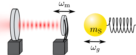
Figure 1: The influence of a time-dependent gravitational acceleration on a Fabry–Pérot moving-end mirror. A small source sphere with mass $m_{\mathrm{S}}$ oscillates with frequency $\omega_{g}$ and creates an oscillating gravitational field, which drives the center of mass motion of the mechanical part of the optomechanical system with frequency $\omega_{\mathrm{m}}$.

Precision measurements of gravitational acceleration – also known as gravimetry – with quantum optomechanical systems in the nonlinear regime have been theoretically considered for measurements of constant gravitational accelerations [25, 26]. However, constant signals are experimentally difficult to detect as they cannot be easily distinguished from a random noise floor. On the other hand, until recently it was not known how to solve the dynamics of fully time-dependent systems in the nonlinear regime. This prevented the careful analysis of the measurement of time-varying signals, which can provide significant advantages through the use of resonant effects.

The closed dynamics of time-dependent optomechanical systems was recently solved in [27, 28], and a general expression for the sensitivity of an optomechanical system with a time-dependent coupling and time-dependent mechanical displacement terms was derived in [29]. In this work, we go beyond the results in [29] by deriving fundamental bounds to measurements of time-dependent gravitational fields and considering enhancements to the fundamental sensitivity. We apply our methods to three specific examples: generic gravimetry of oscillating fields, the detection of the gravitational field from small oscillating source masses, and the detection of gravitational waves. The computations are performed for both coherent and bright squeezed states of the light. We ask whether the intrinsic properties of the optomechanical probe system, such as the form of the light–matter coupling, can be employed to further enhance the sensitivity. This is motivated by the fact that the nonlinearities in the optomechanical coupling can be significantly enhanced by either separately or jointly modulating the mechanical frequency and the light–matter coupling [30, 31]. Such modulations have been demonstrated e.g. in nanomechanical setups [32] or with levitated nanoparticles, such as in hybrid-Paul trap systems [33, 34, 35]. We find that such a modulation, performed at or close to resonance, significantly enhances the system sensitivity. A similar result holds when the trapping frequency is modulated at parametric resonance (twice the mechanical frequency), which has been shown in [36].

To relate our scheme to realistic laboratory measurements, we also compute the sensitivity bounds for homodyne and heterodyne detection of the cavity state. While it was known that homodyne detection is optimal for constant gravitational fields and coherent states of the light in the cavity [25], here we show that it remains optimal for time-varying gravitational fields using initially coherent states of the optical mode (referred to as ’optics’ for short in the following), as well as asymptotically optimal for squeezed states.

The work is structured as follows. In Section II, we introduce the optomechanical Hamiltonian and demonstrate how an external gravitational source enters into the dynamics. We outline the solution to the dynamics in Section II. Following that, we compute the quantum Fisher information for initial coherent states and squeezed states in Section III and discuss when the optical and mechanical degrees-of-freedom disentangle, since this allows us to focus exclusively on the sensitivity based on measurements of the cavity state. We then present our main results, which include expressions for the fundamental sensitivities in Section IV. Next, we consider homodyne and heterodyne measurement schemes in Section V. Finally, we apply our results and consider realistic parameters for three measurement schemes in Section VI: (i) generic gravimetry of time-dependent signals, (ii) detection of gravitational fields from small masses, (iii) and detection of gravitational waves. The paper is concluded with a discussion covering some of the practical implementations of an optomechanical sensor in Section VII and some closing remarks in Section VIII.

II The system

The standard optomechanical Hamiltonian for a single interacting optical and mechanical mode is given by

$$\hat{H}=\hbar\omega_{\mathrm{c}}\,\hat{a}^{\dagger}\hat{a}+\hbar\omega_{\mathrm{m}}\,\hat{b}^{\dagger}\hat{b}-\hbar k\,\hat{a}^{\dagger}\hat{a}\,\bigl{(}\hat{b}^{\dagger}+\hat{b}\bigr{)}\,,$$ (1)

where $\hat{a},\hat{a}^{\dagger}$ and $\hat{b},\hat{b}^{\dagger}$ are the annihilation and creation operators of the cavity field and mechanical oscillator, respectively, satisfying $[\hat{a},\hat{a}^{\dagger}]=1$ and $[\hat{b},\hat{b}^{\dagger}]=1$, where and $\omega_{\mathrm{c}}$ and $\omega_{\mathrm{m}}$ are the optical and mechanical frequencies. The light–matter coupling is denoted by $k$, and its precise form depends on the experimental platform in question.

We consider the case where an external gravitational signal affects the mechanical element, which gives rise to an additional potential term in (1). However, this is not the only change to (1) that we consider, as will become clear later. By expanding the gravitational potential to first order, we obtain the familiar expression $mg(t)\hat{x}_{\mathrm{m}}$, where $g(t)$ is a time-dependent gravitational acceleration and $\hat{x}_{\mathrm{m}}=x_{0}\bigl{(}\hat{b}^{\dagger}+\hat{b}\bigr{)}$ is a linear displacement of the mechanical element, with $x_{0}=\sqrt{\hbar/2m\omega_{\mathrm{m}}}$ the zero-point fluctuation. While generic time-dependent signals can be explored using the methods in [29], here we restrict our analysis to gravitational signals $g(t)$ that are sinusoidally modulated around a constant acceleration, which accounts for all three examples that we model in this work.

We write the gravitational acceleration as

$$g(t)=-g_{0}\left(a+\epsilon\cos(\omega_{g}t+\phi_{g})\right)\,,$$ (2)

where $g_{0}$ is the overall amplitude of the acceleration, $\phi_{g}$ is an arbitrary phase, $a$ is a dimensionless constant contribution, $\epsilon$ is a dimensionless oscillation amplitude, and $\omega_{g}$ is the angular frequency of the signal. This allows us, for example, to model the gravitational field from an oscillating spherical source mass, as illustrated in Figure 1, where $a=1$ and $\epsilon=2\delta r_{0}/r_{0}$, with $\delta r_{0}$ being the amplitude of the time-dependent oscillation and $r_{0}$ the mean separation (see the derivation in Appendix A). We can also use (2) to model gravitational waves (or a set-up mimicking their effects using, for example, moving masses [37]). To do so, we set $a=0$ so that only the oscillating part of the gravitational acceleration remains.

It is well-known that resonances in physical systems can be used to further enhance certain dynamical effects. We therefore make a total of three changes to the standard optomechanical Hamiltonian (1): (i) We add a gravitational term $g(t)$, (ii) we promote the standard constant optomechanical coupling $k$ to a time-dependent one, and (iii) we let the mechanical frequency change as a function of time. The change of the mechanical frequency (iii) can be modelled in two ways: Either by changing the frequency $\omega_{\mathrm{m}}$ and thereby of $\hat{b}$ and $\hat{b}^{\dagger}$, which are defined with respect to this frequency, or by addition of the term $\mathcal{D}_{2}(\tau)(\hat{b}^{\dagger}+\hat{b})^{2}$. In this work, we choose the latter approach, since it allows us to more easily compare this scheme with the previously mentioned cases. The Hamiltonian in the frame rotating with the optical field then becomes

$$\hat{H}=\, \hbar\omega_{\mathrm{m}}\,\hat{b}^{\dagger}\hat{b}-\hbar\omega_{m}\left(k(\tau)\,\hat{a}^{\dagger}\hat{a}-\mathcal{D}_{1}(\tau)\right)\bigl{(}\hat{b}^{\dagger}+\hat{b}\bigr{)}$$

$$\quad+\hbar\omega_{\mathrm{m}}\mathcal{D}_{2}(\tau)\bigl{(}\hat{b}^{\dagger}+\hat{b}\bigr{)}^{2}\;,$$ (3)

where we adopt a rescaled time parameter $\tau=\omega_{\mathrm{m}}t$, and the linear gravitational displacement term $\mathcal{D}_{1}(\tau)$ becomes (given (2))

$$\mathcal{D}_{1}(\tau)=-d_{1}\left(a+\epsilon\cos(\Omega_{d1}\tau+\phi_{d1})\right),$$ (4)

where $\Omega_{d1}=\omega_{g}/\omega_{\mathrm{m}}$, $\phi_{d1}=\phi_{g}$, and where we now identify

$$d_{1}=\frac{mg_{0}}{\hbar\omega_{\mathrm{m}}}\sqrt{\frac{\hbar}{2\omega_{\mathrm{m}}m}}=\frac{g_{0}}{2x_{0}\omega_{\mathrm{m}}^{2}}\,.$$ (5)

The optomechanical coupling $k(\tau)$ depends on the specific system under consideration. For example, for a Fabry–Pérot cavity with a mechanical oscillator mirror, the coupling is a constant, $k(\tau)\equiv k_{0}$ given by $k_{0}=x_{0}\omega_{\mathrm{c}}/(L\omega_{\mathrm{m}})$ [38], where $L$ is the length of the cavity. For levitated dielectric spheres, the coupling takes the form $k_{0}=P\,k_{\mathrm{c}}\,x_{0}\,\omega_{\mathrm{c}}/(2\omega_{\mathrm{m}}\,V_{\mathrm{c}}\,\epsilon_{0})$ [39], where $P$ is the polarizability of the sphere, given by $P=3V\epsilon_{0}(\varepsilon-1)/(\varepsilon+2)$, with volume $V$, relative permittivity $\varepsilon$, and the cavity mode volume $V_{\mathrm{c}}$. Furthermore, $\epsilon_{0}$ is the vacuum permittivity, and $k_{\mathrm{c}}=2\pi/\lambda_{\mathrm{c}}$ is the wave number of the light field. A modulated spring constant $k(\tau)$ is experimentally feasible for Fabry–Pérot systems by positioning an electrode with a time-varying voltage close to the cantilever [40]. For a levitated nanosphere, a similar modulation arises from the natural micromotion that occurs for certain hybrid Paul-trap setups [33, 41]. We later show that a modulation of the light–matter coupling can be used to enhance the sensitivity of the system for measurements of gravitational fields.

II.1 Solution of the dynamics

Our goal now is to solve the dynamics generated by (II). The full solution was developed in [42] and [28]. We briefly review the results here. In general, the time-evolution operator is given by the time-ordered exponential $\hat{U}(\tau)=\overleftarrow{\mathcal{T}}\mathrm{exp}\bigl{[}-i\int^{\tau}_{0}\mathrm{d}\tau\hat{H}(\tau^{\prime})/(\hbar\omega_{\mathrm{m}})\bigr{]}$. By using an approach akin to transforming to the interaction picture, $\hat{U}(\tau)$ can be written as the product

$$\hat{U}(\tau)=\hat{U}_{\mathrm{sq}}(\tau)\,\hat{U}_{\mathrm{NL}}(\tau)\,,$$ (6)

where

$$\hat{U}_{\mathrm{sq}} =\overleftarrow{\mathcal{T}}\mathrm{exp}\Bigg{[}-\frac{i}{\omega_{\mathrm{m}}}\int_{0}^{\tau}\mathrm{d}\tau^{\prime}\left(\hat{N}_{b}+\mathcal{D}_{2}(\tau^{\prime})\left(2\,\hat{N}_{b}+\hat{B}_{+}^{(2)}\right)\right)\Bigg{]}\,,$$

$$\hat{U}_{\mathrm{NL}} =\overleftarrow{\mathcal{T}}\mathrm{exp}\left[-\frac{i}{\omega_{\mathrm{m}}}\int^{\tau}_{0}\mathrm{d}\tau\,\hat{U}_{\mathrm{sq}}^{\dagger}\,\hat{H}_{\mathrm{NL}}(\tau^{\prime})\,\hat{U}_{\mathrm{sq}}\right]\,,$$ (7)

where $\hat{H}_{\mathrm{NL}}=-k(\tau)\hat{a}^{\dagger}\hat{a}\bigl{(}\hat{b}^{\dagger}+\hat{b}\bigr{)}+\mathcal{D}_{1}(\tau)\bigl{(}\hat{b}^{\dagger}+\hat{b}\bigr{)}$, $\hat{N}_{b}=\hat{b}^{\dagger}\hat{b}$, and $\hat{B}_{+}^{(2)}=\hat{b}^{{\dagger}2}+\hat{b}^{2}$. Here, $\hat{U}_{\mathrm{sq}}$ encodes both the free evolution of the mechanical subsystem as well as the term multiplied by $\mathcal{D}_{2}(\tau)$, while $\hat{U}_{\mathrm{NL}}$ contains the remaining nonlinear light–matter interaction term and the gravitational displacement term.

Next, we use a Lie algebra approach to write the remaining time-evolution operator $\hat{U}_{\mathrm{NL}}(\tau)$ as a product of unitary operators. This method was first proposed by Wei and Norman in 1963 [43] and has since been used to solve the dynamics of a large variety of systems [44, 45, 46, 47]. We identify the following Lie algebra of generators, which is closed under commutation:

$$\hat{N}^{2}_{a} :=(\hat{a}^{\dagger}\hat{a})^{2}$$

$$\hat{N}_{a} :=\hat{a}^{\dagger}\hat{a} \hat{N}_{b} :=\hat{b}^{\dagger}\hat{b}$$

$$\hat{B}_{+} :=\hat{b}^{\dagger}+\hat{b} \hat{B}_{-} :=i\,(\hat{b}^{\dagger}-\hat{b})$$

$$\hat{N}_{a}\,\hat{B}_{+} :=\hat{N}_{a}\,(\hat{b}^{\dagger}+\hat{b}) \hat{N}_{a}\,\hat{B}_{-} :=i\,\hat{N}_{a}\,(\hat{b}^{\dagger}-\hat{b}).$$ (8)

Similarly, it is possible to find a Lie algebra that generates the time-evolution encoded in $\hat{U}_{\mathrm{sq}}$. It is made up of the following operators [28]: $\hat{N}_{b}$, $\hat{B}_{+}^{(2)}=\hat{b}^{{\dagger}2}+\hat{b}^{2}$, and $\hat{B}_{-}^{(2)}=i\bigl{(}\hat{b}^{{\dagger}2}-\hat{b}^{2}\bigr{)}$.

Identifying the Lie algebra enables us to write down the following Ansätze for the two time-evolution operators [28]

$$\hat{U}_{\mathrm{sq}}(\tau)=\, e^{-i\,J_{b}\,\hat{N}_{b}}\,e^{-i\,J_{+}\,\hat{B}_{+}^{(2)}}\,e^{-i\,J_{-}\,\hat{B}_{-}^{(2)}}\,,$$ (9)

$$\hat{U}_{\mathrm{NL}}(\tau)=\, e^{-i\,F_{\hat{N}_{a}}\,\hat{N}_{a}}\,e^{-i\,F_{\hat{N}^{2}_{a}}\,\hat{N}^{2}_{a}}\,e^{-i\,F_{\hat{B}_{+}}\,\hat{B}_{+}}$$

$$\times\,e^{-i\,F_{\hat{N}_{a}\,\hat{B}_{+}}\,\hat{N}_{a}\,\hat{B}_{+}}\,e^{-i\,F_{\hat{B}_{-}}\,\hat{B}_{-}}\,e^{-i\,F_{\hat{N}_{a}\,\hat{B}_{-}}\,\hat{N}_{a}\,\hat{B}_{-}}\,.$$

By now equating the two Ansätze (9) with their respective expressions in (II.1) and differentiating on both sides, we can use the linear independence of the operators to obtain a number of differential equations. Solving these, we find that the $F$ coefficients are given by integrals shown in (B) in Appendix B, and the $J$ coefficients are similarly given by the expressions in (B). For explicit expressions of the functions $k(\tau)$, $\mathcal{D}_{1}(\tau)$ and $\mathcal{D}_{2}(\tau)$, it is then possible to solve the system either exactly or numerically.

In this work, we draw on analytic and perturbative solutions developed in Refs [28] and [29], which are briefly outlined in Appendix B.

II.2 Initial states of the system

It is well-known that the fundamental sensitivity of a detector depends on the initial state of the system, and that significant enhancements can be gained through the use of non-classical states. For optomechanical systems, ground-state cooling has been demonstrated for a number of platforms [48, 49, 50, 24], however, the most realistic and practical state of the mechanical oscillator is a thermal state. The total initial state of the system is

$$\hat{\rho}(0)=\ket{\psi_{\mathrm{c}}}\bra{\psi_{\mathrm{c}}}\otimes\sum_{n=0}^{\infty}\frac{\tanh^{2n}r_{T}}{\cosh^{2}r_{T}}\ket{n}\bra{n}\,,$$ (10)

where $\ket{\psi_{\mathrm{c}}}$ is the initial optical state of the cavity and the parameter $r_{T}$ is defined by the relation $r_{T}=\mathrm{tanh}^{-1}(\exp[-\hbar\,\omega_{\textrm{m}}/(2\,k_{\textrm{B}}\,T)])$, for which $k_{\mathrm{B}}$ is Boltzmann’s constant and $T$ is the temperature.

In this work, we consider two different cavity states:

• A coherent state $\ket{\mu_{\textrm{c}}}$ (accessible through laser driving), where $\hat{a}\ket{\mu_{\textrm{c}}}=\mu_{\textrm{c}}\ket{\mu_{\textrm{c}}}$. The average number of photons in the cavity is $|\mu_{\mathrm{c}}|^{2}$.

• A squeezed coherent state $\ket{\zeta,\mu_{\mathrm{c}}}=\hat{S}_{\zeta}\ket{\mu_{\mathrm{c}}}$ (also known as “bright squeezed state”) where $\hat{S}_{\zeta}=\mathrm{exp}\left[(\zeta^{*}\hat{a}^{2}-\zeta\hat{a}^{{\dagger}2})/2\right]$ with $\zeta=re^{i\varphi}$. These states can be prepared through parametric down-conversion [51], or four-wave mixing in an optical cavity [52], and they have recently been used to improve the sensitivity of LIGO [13]. Currently, squeezed optical states with $r=1.42$ [53, 54] and even $r=1.73$ [55] have been achieved in the laboratory.

It is known that a Fock state superposition given by $(\ket{0}+\ket{n})/\sqrt{2}$, where $\hat{a}^{\dagger}\hat{a}\ket{n}=n\ket{n}$ can be used to maximise the sensitivity of the system for a given maximum excitation $n$ [56, 57]. However, it is difficult to prepare states with large $n$ (currently, $n=4$ has been experimentally demonstrated [58]), and we therefore focus on (squeezed) coherent states in this work.

III Quantum metrology of linear displacements

We are interested in the fundamental limits that optomechanical systems can achieve when sensing displacements due to gravity. For this purpose, we turn to tools in quantum metrology.

III.1 Quantum Fisher information

In general, quantum metrology provides an ultimate bound on the precision of measurements of a classical parameter $\theta$. If $\theta$ parametrises a unitary quantum channel $\hat{U}_{\theta}$, it is coded into the state as $\hat{\rho}_{\theta}=\hat{U}_{\theta}\,\hat{\rho}_{\mathrm{in}}\,\hat{U}^{\dagger}_{\theta}$ [12]. Then, given a specific input state $\hat{\rho}_{\textrm{in}}$, it is possible to compute the quantum Cramér-Rao bound (QCRB), which reads

$$\mathrm{Var}(\theta)\geq\frac{1}{\mathcal{M}\,\mathcal{I}},$$ (11)

where $\mathcal{I}$ is the quantum Fisher information (QFI) for the parameter $\theta$ and $\mathcal{M}$ is the number of measurements, or input probes [59]. The QCRB bound is optimised over all possible (POVM) measurements and data analysis schemes with unbiased estimators, and can be saturated in the limit of $\mathcal{M}\rightarrow\infty$.

For a unitary channel $\hat{U}_{\theta}$, and for a mixed initial state given by $\hat{\rho}(0)=\sum_{n}\lambda_{n}\ket{\lambda_{n}}\bra{\lambda_{n}}$ the QFI is given by [60, 61]:

$$\mathcal{I}= \;4\sum_{n}\lambda_{n}\,\left(\bra{\lambda_{n}}\mathcal{\hat{H}}_{\theta}^{2}\ket{\lambda_{n}}-\bra{\lambda_{n}}\mathcal{\hat{H}}_{\theta}\ket{\lambda_{n}}^{2}\right)$$

$$\quad-8\sum_{n\neq m}\frac{\lambda_{n}\lambda_{m}}{\lambda_{n}+\lambda_{m}}\bigl{|}\bra{\lambda_{n}}\mathcal{\hat{H}}_{\theta}\ket{\lambda_{m}}\bigr{|}^{2},$$ (12)

where $\hat{\mathcal{H}}_{\theta}=-i\hat{U}_{\theta}^{\dagger}\partial_{\theta}\hat{U}_{\theta}$. In our case, $\hat{U}_{\theta}$ is the time-evolution operator in (6), which results from a gravitational signal affecting the optomechanical system. The general form for the global QFI for the Hamiltonian (II) was computed in [29].

We are interested in estimating parameters that appear in the displacement function $\mathcal{D}_{1}(\tau)$, which arises from the gravitational signal. We therefore pick $d_{1}$ in (4) as our fiducial estimation parameter, and by the chain-rule, we can choose to estimate any parameter that appears in $d_{1}$. With this choice, only three dynamical coefficients, $F_{\hat{N}_{a}}$, $F_{\hat{B}_{+}}$, and $F_{\hat{B}_{-}}$, contain the function $\mathcal{D}_{1}$ (see (B) in Appendix B), meaning that all other coefficients are zero when differentiated with respect to $d_{1}$.

It follows from equation (9) in [29] that the operator $\hat{\mathcal{H}}_{d1}$ is given by

$$\hat{\mathcal{H}}_{d1}=B\hat{N}_{a}+C_{+}\hat{B}_{+}+C_{-}\hat{B}_{-},$$ (13)

where $B$ and $C_{\pm}$ are coefficients defined by

$$B= -\partial_{d_{1}}F_{\hat{N}_{a}}-2\,F_{\hat{N}_{a}\,\hat{B}_{-}}\partial_{d_{1}}F_{\hat{B}_{+}}\;,$$

$$C_{\pm}= \,-\partial_{d_{1}}F_{\hat{B}_{\pm}}\;.$$ (14)

The global QFI takes the form (see the derivation in Appendix C):

$$\mathcal{I}=4\left[B^{2}(\Delta\hat{N}_{a})^{2}+\mathrm{sech}(2r_{T})\left(C_{+}^{2}+C_{-}^{2}\right)\right],$$ (15)

where the variance of $\hat{N}_{a}$, $(\Delta\hat{N}_{a})^{2}\equiv\mathrm{Var}(\hat{N}_{a})=\braket{\hat{N}_{a}^{2}}-\langle\hat{N}_{a}\rangle^{2}$, and where the bracket $\braket{\cdot}$ denotes the expectation value with respect to one of the initial states presented in Section II.2. For the coherent state and the squeezed state, we find (see Appendix C):

$$(\Delta\hat{N}_{a})_{\mu_{\mathrm{c}}}^{2}= \,|\mu_{\mathrm{c}}|^{2}\,,$$ (16)

$$(\Delta\hat{N}_{a})_{\mu_{\mathrm{c}},\zeta}^{2}= \,\left|\mu_{\mathrm{c}}\right|^{2}e^{4r}+\frac{1}{2}\sinh^{2}(2r)\,$$

$$-2\mathfrak{R}[e^{-\frac{i\varphi}{2}}\mu_{\mathrm{c}}]^{2}\sinh(4r)\,,$$ (17)

where we recall that $r$ and $\varphi$ are the squeezing parameters given by $\zeta=re^{i\varphi}$. The angle $\varphi$ is defined with respect to the coherent state phase. The case of coherent states ($r=0$) was considered previously in [25, 26, 29].

For coherent states, a higher photon number $|\mu_{\mathrm{c}}|^{2}$ yields a better sensitivity. For squeezed coherent states, the QFI is maximised when $e^{\frac{i\varphi}{2}}\mu_{\mathrm{c}}$ is purely imaginary, and when the photon number $|\mu_{\mathrm{c}}|^{2}$ and $r$ are maximised. In each case, the increase in sensitivity is not without cost, as there are certain restrictions to how much the mechanical element can be displaced. See Section VII.5 for a discussion of these restrictions, where we also propose order-of-magnitude limitations for the parameters of the cavity field.

Once the QFI has been computed, we can obtain the optimal measurement sensitivity through the QCRB. Given the dimensionless expression (4), we use the chain-rule to find that the sensitivity $\Delta g_{0}$ to the gravitational amplitude $g_{0}$ (see the expression in (2)) is

$$\Delta g_{0}\geq\left|\frac{\mathrm{d}}{\mathrm{d}g_{0}}d_{1}\right|^{-1}\frac{1}{\sqrt{\mathcal{M}\,\mathcal{I}}}=\frac{2x_{0}\omega_{\mathrm{m}}^{2}}{\sqrt{\mathcal{M}\,\mathcal{I}}}\,.$$ (18)

In Section V, we consider the classical Fisher information (CFI), which provides the sensitivity given a specific measurement. We now turn to the question of optimal timing of the measurement.

III.2 Disentangling of the optics and mechanics

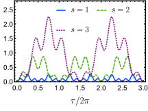
(a)

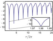
(b)

Figure 2: Disentangling conditions for the light and mechanics. When the function $|K_{\hat{N}_{a}}|^{2}=F_{\hat{N}_{a}\,\hat{B}_{-}}^{2}+F_{\hat{N}_{a}\,\hat{B}_{+}}^{2}$ is zero, the state is separable. (a) is a plot of $|K_{\hat{N}_{a}}|^{2}$ (shown in (D)) for a modulated optomechanical coupling (specified in (21)) with different frequencies $\Omega_{\mathrm{frac}}=1+2n_{1}/s$ and with $k_{0}=n_{1}=1$. The resonant case $\Omega_{k}=1$ (not shown) never evolves into a separable state, while $|K_{\hat{N}_{a}}|^{2}$ vanishes at multiples of $\tau=s\pi$ for $\Omega_{\mathrm{frac}}=3$ (blue solid line), $\Omega_{\mathrm{frac}}=2$ (green dashed line), and $\Omega_{\mathrm{frac}}=5/3$ (magenta dotted line). (b) is a plot of $2\log|K_{\hat{N}_{a}}|$ for a modulated squeezing with $d_{2}=0.01$ and a constant optomechanical coupling $k_{0}=1$. At no point within the shown time interval does the states evolve into a separable state.

For Hamiltonians such as (II), it is well-known that the optical and mechanical subsystems evolve into an entangled state [62], however, for particular choices of the dynamics, we find that there are certain times when the two systems end up in a separable state. This is a consequence of the unitary dynamics, and we refer to these times as $\tau_{\mathrm{sep}}$.

In an experiment, it is often the case that an observable on the cavity state is measured. If we can identify the disentangling conditions and hence $\tau_{\mathrm{sep}}$, we can immediately compute the QFI of the cavity state at these separation times. It was also previously found that the global QFI peaks when the states are separable, and that the noise contained in an initially thermal mechanical state also does not affect the sensitivity at this time [25, 29].

From (6), we note that only the exponentials with $F_{\hat{N}_{a}\,\hat{B}_{+}}$ and $F_{\hat{N}_{a}\,\hat{B}_{-}}$ mediate entanglement between the cavity field and the mechanics, since their accompanying generators $\hat{N}_{a}\,\hat{B}_{+}$ and $\hat{N}_{a}\,\hat{B}_{-}$ encode an interaction between the light and mechanical oscillator (referred to as ’mechanics’ for short in the following). We therefore construct the function $K_{\hat{N}_{a}}=F_{\hat{N}_{a}\,\hat{B}_{-}}+iF_{\hat{N}_{a}\,\hat{B}_{+}}$, and express a sufficient condition for separability as

$$|K_{\hat{N}_{a}}|^{2}=F_{\hat{N}_{a}\,\hat{B}_{-}}^{2}+F_{\hat{N}_{a}\,\hat{B}_{+}}^{2}=0\,.$$ (19)

When this condition is fulfilled, the full time-evolution operator $\hat{U}(\tau)$ factorises into terms that act exclusively on the optical and mechanical states. The part acting on the cavity state is given by $\hat{U}_{\mathrm{c}}(\tau)=\hat{U}_{\mathrm{sq}}(\tau)\,e^{-i\,F_{\hat{N}_{a}^{2}}\,\hat{N}_{a}^{2}}\,e^{-i\,F_{\hat{N}_{a}}\,\hat{N}_{a}}$. For later, we note that, when applied to a coherent state $\ket{\mu_{\mathrm{c}}}$, the last exponential induces a phase, such that the new coherent state parameter is $\tilde{\mu}_{\mathrm{c}}=\mu_{\mathrm{c}}\,e^{-iF_{\hat{N}_{a}}}$. This definition will become useful to us when we discuss homodyne measurements of the cavity field in Section V.

The advantage of identifying the conditions for $|K_{\hat{N}_{a}}|^{2}=0$ is that we can derive an analytic expression for the fundamental sensitivity that can be achieved by measuring the cavity state. We also do not have to concern ourselves with any contributions from the initial thermal mechanical state. The QFI of the optical state is then simply (from (III.1) and (15)):

$$\mathcal{I}_{\mathrm{c}}=4\,(\partial_{d_{1}}F_{\hat{N}_{a}})^{2}(\Delta\hat{N}_{a})^{2}\,,$$ (20)

where we use the subscript ‘c’ to denote the fact that this refers to the QFI of the cavity state only.

To determine when the condition in (19) is satisfied, we must evaluate the expression for a given dynamics. Firstly, we note that the form of the gravitational acceleration (determined by the function $\mathcal{D}_{1}(\tau)$) does not affect the entanglement between the systems. This is because $\mathcal{D}_{1}(\tau)$ does not feature in the integrals for $F_{\hat{N}_{a}\,\hat{B}_{+}}$ and $F_{\hat{N}_{a}\,\hat{B}_{-}}$ (see the expressions in (B)).

In contrast, the optomechanical coupling $k(\tau)$ and the squeezing function $\mathcal{D}_{2}(\tau)$ completely determine the times $\tau_{\mathrm{sep}}$ at which the two systems become separable. For a constant optomechanical coupling $k(\tau)\equiv k_{0}$, the states reach their maximum entanglement at $\tau=\pi$, after which they return to a separable state at $\tau_{\mathrm{sep}}=2\pi$ [62, 25]. We can prove this explicitly by computing $F_{\hat{N}_{a}\,\hat{B}_{+}}$ and $F_{\hat{N}_{a}\,\hat{B}_{-}}$ for a constant coupling, and we find that $|K_{\hat{N}_{a}}|^{2}=2k_{0}^{2}(1-\cos(\tau))$, which vanishes when $\tau$ is a multiple of $2\pi$.

When the coupling $k(\tau)$ is time-dependent, however, the behaviour of the system – and the entanglement – becomes richer. As we are interested in whether a modulated coupling can lead to resonance type enhancements, a natural choice is to assume it takes on the form [31]

$$k(\tau)=k_{0}\cos(\Omega_{k}\tau+\phi_{k})\,,$$ (21)

where $\Omega_{k}$ is the oscillation frequency divided by $\omega_{\mathrm{m}}$ and $\phi_{k}$ is an arbitrary phase. For zero mechanical squeezing ($\mathcal{D}_{2}=0$), the $F$-coefficients are given in (B.2), and $K_{\hat{N}_{a}}$ is given in (D). When the optomechanical coupling is modulated at resonance with $\Omega_{k}=1$, we find that the light and mechanical oscillator never disentangle. This means that we cannot ignore the mechanical contribution to the QFI, and since computing the QFI for a reduced state is challenging, we resort to the global expression in (15) as an upper bound.

A key observation however, is that for specific choices of the coupling modulation frequencies, the light and mechanics do disentangle at certain points in the evolution. In Appendix D we prove that when the frequencies take on a fractional form, $\Omega_{\mathrm{frac}}=1+2n_{1}/s$ , for $n_{1}$ and $s$ integers ($s$ positive), the subsystems decouple at times that are multiples of $\tau_{\mathrm{sep}}=s\pi$. This means that the QFI for the cavity state is given again by (20).

Finally, for a mechanical frequency modulated with $\mathcal{D}_{2}=d_{2}\cos(2\tau+\phi_{d2})$, we find no point where the system is completely separable (see Figure 2b).

IV Gravimetry of time-dependent gravitational fields

We are now in a position to evaluate the QFI explicitly for a number of cases of interest. Throughout, we assume that the gravitational signal is given by the time-dependent expression in (4). Further, we keep the optomechanical coupling constant for now with $k(\tau)\equiv k_{0}$, and we assume that the mechanical squeezing is zero. In Section III.2, we showed that for this choice of dynamics, the light and mechanical oscillator disentangle whenever the time $\tau$ is a multiple of $2\pi$.

We therefore find that (see Appendix C.2), at resonance with $\Omega_{d1}=1$, and at time $\tau_{\mathrm{c}}=2n\pi$ with integer $n$, the global QFI becomes

$$\mathcal{I}^{(\Omega_{d1}=1)}= \,4\,\pi^{2}\,n^{2}\,k_{0}^{2}\,(\Delta\hat{N}_{a})^{2}(2a-\epsilon\cos(\phi_{d1}))^{2}$$

$$+(2\pi n)^{2}\epsilon^{2}\text{sech}(2r_{T})\,,$$ (22)

which is maximized over $\phi_{d1}$ for $\phi_{d1}=\pi$. This is a phase relation between the driving signal, which excites oscillations of the mechanics, and the light–matter coupling term, which fixes the decoupling times. The much longer form of the QFI for a general frequency $\Omega_{d1}$ is shown in (C.2) in Appendix C.

In a classical setting, we expect that driving the mechanical element on resonance will rapidly increase its oscillation amplitude, which means that it becomes easier and easier to detect its displacement. We do see this increase in the $\sim n^{2}$-scaling of the second term of (IV). However, this term is usually small compared with the first term, since both scale with $\sim n^{2}$ and the first term scales with the photon number variance $(\Delta\hat{N}_{a})^{2}$.

To focus on this point, we consider the cavity state QFI (20) at times when the light and mechanics evolve into a separable state. For a purely oscillating field with $a=0$, the local QFI for measurements of the cavity field becomes

$$\mathcal{I}_{\mathrm{c}}^{(\Omega_{d1}=1)}=(4\pi n)^{2}\,k_{0}^{2}\,\epsilon^{2}\,(\Delta\hat{N}_{a})^{2}\,.$$ (23)

When $\epsilon=1$, this is in fact smaller than the constant driving scenario (with $a=1$) by a factor of $4$. So, while resonant driving does increase the global and local QFI over time, as one would intuitively expect, this is primarily through the amplitude change of the mechanical element. As such, it does not translate directly to observations on the cavity field. It turns out, however, that an analogous enhancement can be passed to the field provided modulations are introduced to the system in a different way. In this section we consider two additional methods by which this can be done: Modulating the optomechanical light–matter interaction, and modulating the trapping frequency. We return to (23) later on and use it to compare the effects of the enhancements.

We also note here that when the optical and mechanical elements are disentangled, the sensitivity that can be obtained from the cavity state alone does not depend on the thermal noise present in the initial mechanical state. For non-unitary dynamics, however, we expect the system to thermalise and decohere, which generally prevents the subsystems from completely disentangling.

IV.1 Enhanced sensing through optomechanical modulation

We are interested in whether the form of the light–matter coupling $k(\tau)$ can be used to enhance the sensitivity of the system. Such a time-modulated coupling has been experimentally demonstrated [40, 32, 63]. We specifically consider a coupling of the form shown in (21). The global QFI for a resonant gravitational signal at arbitrary times can be found in (C.3), and it is dominated by terms proportional to $n^{4}$ for large $\tau$ when $(\phi_{d1}-\phi_{k})/\pi$ is not an integer. Should coherence be maintained for long periods of time, the resonantly modulated coupling leads to rapid increases in the measurement precision.

For mechanical resonance ($\Omega_{k}=\Omega_{d1}=1$), we noted before that the light and the mechanics do not disentangle at all. This means that the QFI is global at all times, and therefore does not necessarily reflect the sensitivity that could be realistically obtained in the laboratory through measurements of the optical state. For multiples of the mechanical period, $\tau_{c,n}=2\pi n$, the global QFI becomes,

$$\mathcal{I}^{(\Omega_{d1,k}=1)} =\pi^{2}n^{2}k_{0}^{2}\,(\Delta\hat{N}_{a})^{2}\Big{[}4a\cos(\phi_{k})$$ (24)

$$+\epsilon\Big{(}2\pi n\sin(\phi_{d1}-\phi_{k})+2\cos(\phi_{d1}+\phi_{k})$$

$$\quad-\cos(\phi_{d1}-\phi_{k})\Big{)}\Big{]}^{2}+(2\pi n)^{2}\epsilon^{2}\text{sech}(2r_{T})\,.$$

The full expression for arbitrary $\tau$ is given in (C.3). We note that the term multiplied by $\epsilon$ provides an additional scaling with $n^{2}$, leading to an overall scaling of $n^{4}$. Such an enhancement is only present when the gravitational field is oscillating with nonzero $\epsilon$, and indicates that the two resonances (the gravitational signal and the optomechanical coupling, resonant with the mechanical frequency) constructively enhance the sensitivity. This is optimised when $\phi_{d1}-\phi_{k}=\pi/2$. Furthermore, the term multiplied by $a$ is maximised for $\phi_{k}=0$, so we can choose $\phi_{d1}=\pi/2$ to optimise the expression.

For a purely oscillating gravitational field $a=0$ and a large temperature $r_{T}\rightarrow\infty$, then setting $\phi_{d1}=\pi/2$ and $\phi_{k}=0$, simplifies the expression in (24) to

$$\mathcal{I}^{(\Omega_{\mathrm{d1},k}=1)}=4\pi^{4}n^{4}k_{0}^{2}\,\epsilon^{2}\,(\Delta\hat{N}_{a})^{2},$$ (25)

which, compared with a constant coupling, is an improvement of $\sim n^{2}\pi^{2}/4$ for purely oscillating fields (23).

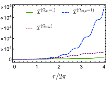
(a)

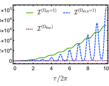
(b)

Figure 3: The quantum Fisher information for detecting linear displacements with a modulated optomechanical system. We choose the example values $r_{T}\rightarrow\infty$, $k_{0}=1$, $\mu_{\mathrm{c}}=1$, and $re^{i\varphi}=1$ in both plots in order to compare the different schemes. (a) shows the QFI for a purely oscillating gravitational field with $a=0$ and $\epsilon=1$. We compare the global QFI for a resonant gravitational signal $\mathcal{I}^{(\Omega_{d1}=1)}$ in (IV) (green solid line) with the enhanced global QFI for a modulation of the optomechanical coupling at resonance ($\Omega_{d1}=\Omega_{k}=1$) denoted by $\mathcal{I}^{(\Omega_{d1,k}=1)}$ in (C.3) (blue dashed line), and the enhanced QFI for fractional frequencies $\Omega_{d1}=\Omega_{k}=\Omega_{\mathrm{frac}}=1+2n_{1}/s$ denoted by $\mathcal{I}^{(\Omega_{\mathrm{frac}})}$ in (C.3) (dotted purple line), where we set $n_{1}=-1$ and $s=8$ for this plot. The phases have been chosen such that they optimise the QFI for each case (see the main text). The QFI for a resonant coupling shows the strongest increase for later times, but the states never disentangle, which means that we can only upper bound the sensitivity for a measurement of the optical field alone. (b) shows the global QFI for a constant plus oscillating gravitational field with $a=1$ and $\epsilon=0.1$, where we estimate the overall amplitude $d_{1}$. The fractional frequencies no longer perform well because $\epsilon\ll a$, however the scaling with the parameter $s$ can only be appreciated when comparing the curves for different fractional frequencies. Resonant gravimetry, denoted by $\mathcal{I}^{(\Omega_{d1}=1)}$, increases smoothly but it is outperformed by modulated resonant gravimetry $\mathcal{I}^{(\Omega_{d1,k}=1)}$ for large $\tau$.

The global QFI is generally not accessible in an experimental setting, since it is difficult to measure the mechanical element directly. However, we saw in Section III.2 that the light and mechanical oscillator become separable for very specific choices of the frequency $\Omega_{k}$, which we referred to as the fractional frequencies $\Omega_{\mathrm{frac}}$. With this choice, we compute the local QFI for the cavity state with $\Omega_{k}=\Omega_{d1}=\Omega_{\mathrm{frac}}$. Using the expression for the cavity state QFI in (20), we find that when $\Omega_{\mathrm{frac}}=1+2n_{1}/s$, with $s>$ being a positive integer and integer $n_{1}\neq 0$ with $2n_{1}/s>-1$, the QFI becomes, at $\tau_{\mathrm{sep}}=q\,s\pi$, where $q$ is a positive integer:

$$\mathcal{I}_{\mathrm{c}}^{(\Omega_{d1,k}=\Omega_{\mathrm{frac}})}= \,\frac{k^{2}_{0}(\Delta\hat{N}_{a})^{2}s^{2}}{4n_{1}^{2}(n_{1}+s)^{2}(2n_{1}+s)^{2}}$$ (26)

$$\times\bigl{[}\pi qs^{2}\epsilon(2n_{1}+s)\cos(\phi_{d1}-\phi_{k})$$

$$\quad-8an_{1}\left((-1)^{qs}-1\right)(n_{1}+s)\sin(\phi_{k})\bigr{]}^{2}\,.$$

For a purely oscillating signal with $a=0$, the optimal choice of phases $\phi_{d1}-\phi_{k}=0$, and $n_{1}=-1$ (which means that $\Omega_{\mathrm{frac}}=1-2/s$ and $s\geq 3$), we find that the optimal choice for $q$ and $s$ for a given disentangling time $\tau_{\mathrm{sep}}=q\,s\pi$ is to maximise $s$ which implies $q=1$. Then, the QFI becomes

$$\mathcal{I}_{\mathrm{c}}^{(\Omega_{d1,k}=\Omega_{\mathrm{frac}})} =\frac{\pi^{2}\,k_{0}^{2}\,\epsilon^{2}\,s^{6}}{4(1-s)^{2}}(\Delta\hat{N}_{a})^{2}\,.$$ (27)

Equation (27) is one of the main results in this paper, since it provides a sensitivity that can be realistically achieved from measurements on the cavity state alone.

To see how well the enhancement compares, we contrast $\mathcal{I}^{(\Omega_{d1,k}=\Omega_{\mathrm{frac}})}$ with (23). Note that $n$ is the parameter giving the number of mechanical periods. The meaning of $s$ is different; it is the parameter defining the fractional frequency. Using (27), and assuming that $s$ is even, such that $s=2n$, we find an improvement of $\sim n^{2}/4$ for $s\gg 1$.

For arbitrary times, we refer to Figure 3, which shows the general behaviour of the global QFI. The plot in 3a compares resonant gravimetry $\mathcal{I}^{(\Omega_{d1}=1)}$ with the enhancements $\mathcal{I}^{(\Omega_{d1,k}=1)}$ and $\mathcal{I}^{(\Omega_{d1,k}=\Omega_{\mathrm{frac}})}$ obtained by including a time-dependent coupling $k(\tau)$ for purely oscillating gravitational fields, and the plot in 3b shows the same quantities for a gravitational field with constant and oscillating parts. In both plots, we consider large temperatures with $r_{T}\rightarrow\infty$, (which minimises any additional information which can be gained from the mechanics), and set $k_{0}=(\Delta\hat{N}_{a})^{2}=1$, since these are merely multiplicative factors in the QFI. We also choose the optimal phases for each setting, which are $\phi_{d1}=\pi$ for $\mathcal{I}^{(\Omega_{d1}=1)}$, $\phi_{d1}=0$ and $\phi_{k}=\pi/2$ for $\mathcal{I}^{(\Omega_{d1,k}=1)}$, and finally $\phi_{d1}=\phi_{k}=\pi/2$ for $\mathcal{I}^{(\Omega_{\mathrm{frac}})}$.

IV.2 Enhanced sensing through modulated mechanical frequency

The second enhancement we consider (separately from the above) is the inclusion of a mechanical squeezing term $\mathcal{D}_{2}(\tau)\bigl{(}\hat{b}^{{\dagger}2}+\hat{b}^{2}\bigr{)}$. We assume that it is periodically modulated with

$$\mathcal{D}_{2}(\tau)=d_{2}\cos(\Omega_{d2}\tau+\phi_{d2})\,,$$ (28)

where $d_{2}$ is the amplitude, $\Omega_{d2}$ is the rescaled modulation frequency and $\phi_{d2}$ a phase factor.

A term of this form can be generated by, for example, modulating the spring constant [31] or the trapping frequency of a levitated system [34, 35]. In particular, in the levitated systems presented in [33, 34, 35], modulations of the light-matter coupling are always accompanied by a modulation of the mechanical frequency.

When $\Omega_{d2}=2$, this corresponds to a parametric amplification of the mechanical oscillation and leads to a squeezed state of the mechanics (see [64] for how this can be implemented experimentally). The perturbative solutions of the dynamics were found in [28], and are valid for $d_{2}\ll 1$ and $d_{2}\tau$ of order (at most) one. This means that we can only consider small values of $d_{2}$, especially if we are interested in large times $\tau$.

When the mechanical trapping frequency is modulated sinusoidally, the light and mechanics never disentangle, and we are therefore unable to consider the QFI of the optical state separately (see Section III.2 and Figure 2b). We therefore resort to the global QFI in (15). The modulation of the mechanical frequency leads to an enhancement of the QFI depending on the phases $\phi_{d1}$ and $\phi_{d2}$, however the full expression is long and cumbersome. We refer to Appendix C.4, and instead find the optimal phase choice numerically. From the QFI plotted in Figure 4, we see that the choice of $\phi_{d2}=-\pi/2$ and $\phi_{d1}=0$ maximises the QFI.

With this choice of phases, taking into account that $d_{2}\tau\sim 1$ and $d_{2}\ll 1$, the dominating term in the QFI is

$$\mathcal{I}^{(\Omega_{d2}=2)}\approx\frac{4k_{0}^{2}\epsilon^{2}\left(e^{d_{2}\tau}-1\right)^{2}}{d_{2}^{2}}(\Delta\hat{N}_{a})^{2}\,.$$ (29)

Compared with the QFI for resonant gravimetry without any enhancements in (23), the modulated mechanical frequency brings an improvement of $\sim(e-1)^{2}\sim 3$ when $d_{2}\tau\sim 1$, and $\tau=2\pi$. This means that the addition of a modulated squeezing term can increase the sensitivity, but we are limited by our perturbative method in predicting its efficiency.

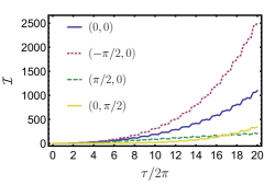
Figure 4: The plot shows the exact QFI $\mathcal{I}^{(\Omega_{d2}=2)}$ for the sensing of a purely oscillating gravitational field (i.e. $a=0$) for different values for the initial phase parameters of frequency modulation and gravity oscillation $(\phi_{d2},\phi_{d1})$. The gravitational field is modulated on resonance $(\Omega_{d1}=1)$ and the mechanical frequency is modulated on parametric resonance $(\Omega_{d2}=2)$. For the plots, we used the parameter values $k_{0}=1$, $\epsilon=1$, $d_{2}=0.02$, $\mu_{\mathrm{c}}=1$ and no squeezing of the cavity field. However, $k_{0}$, $\epsilon$ and $\mu_{\mathrm{c}}$ appear only if $r_{T}$ is very large, as we assumed. Therefore, the only relevant parameter is $d_{2}$, which defines the time-scale on which the effect of parametric driving becomes pronounced.

The inclusion of a constant squeezing term $\mathcal{D}_{2}\equiv d_{2}$ is equivalent to changing the mechanical frequency as $\omega_{\mathrm{m}}\rightarrow\omega_{\mathrm{m}}\sqrt{1+4\mathcal{D}_{2}}$. Since the dimensionful QFI scales with $\omega_{\mathrm{m}}^{-5}$  , larger $d_{2}$ means that the QFI decreases.

V Homodyne and heterodyne metrology of linear displacements

While the QFI and the QCRB provide the ultimate limits to how well a parameter can be estimated, it is not immediately clear which measurements actually saturate this bound. Experimentally, one would almost always measure the optical state using a homodyne measurement, a heterodyne measurement, or photon counting.

The cavity field as present in our description is not directly experimentally accessible, although the contrary is commonly assumed in the literature. To build on these results, one would have to consider output fields leaking from the cavity, which we leave to future work. Instead, here we compute the classical Fisher information (CFI) for these ideal measurements on the cavity state, focusing on when the light and mechanics have disentangled (see Section III.2).

When the light mode and mechanical oscillator are in a separable state, the local QFI generator reduces to $\hat{\mathcal{H}}_{d1}=B\hat{N}_{a}$, where $B$ is defined in (III.1). The optimal bound is given by the QFI in (20), and our aim is to investigate whether a homodyne or heterodyne measurement satisfies this.

The general expression for the CFI is

$$I=\int\mathrm{d}x\frac{1}{p(x,d_{1})}\left(\frac{\partial p(x,d_{1})}{\partial d_{1}}\right)^{2}\,,$$ (30)

where we henceforth denote all CFI quantities by $I$, rather than $\mathcal{I}$, which we reserve for the QFI, and where $p(x,d_{1})=\mathrm{Tr}\bigl{[}\hat{\rho}_{d1}\,\hat{\Pi}_{x}\bigr{]}$ is a probability distribution resulting from a measurement with a POVM element $\hat{\Pi}_{x}$. Assuming that the initial cavity-field state is pure (which in the settings we consider here is always true when the optics and mechanics are separable), we define the state $\ket{\psi_{\tau}}=\hat{U}_{\mathrm{c}}\ket{\psi_{0}}$, where $\hat{U}_{\mathrm{c}}=e^{-iF_{\hat{N}_{a}}\hat{N}_{a}}\,e^{-i\,F_{\hat{N}_{a}^{2}}\hat{N}_{a}^{2}}$ acts on the cavity state. Then, noting that the probability is given by $p(x)=|\langle\psi_{\tau}|x\rangle|^{2}$ and $\mathds{1}=\int dx\ket{x}\!\!\bra{x}$, the CFI can be written,

$$I=2\,B^{2}\braket{\hat{N}_{a}^{2}}-(R+R^{*})\,,$$ (31)

where

$$R =B^{2}\int dx\left(\frac{\langle x|\hat{N}_{a}|\psi_{\tau}\rangle}{\langle x|\psi_{\tau}\rangle}\right)^{2}p(x)\,.$$ (32)

The first term in (31) is relatively straightforward to calculate, however, it is generally difficult to perform the integral in (32). A particular simplification exists when $\langle x|\hat{N}_{a}|\psi_{\tau}\rangle$ is proportional to $\langle x|\psi_{\tau}\rangle$. This occurs, for example, when the state at $\tau={\tau_{\text{sep}}}$ is a coherent state, which can be guaranteed by choosing parameters such that the coefficient $F_{\hat{N}_{a}^{2}}$ is a multiple of $2\pi$ at the disentangling time (see Appendix E for details). For mathematical convenience we will make this assumption in the remainder of this section, however it turns out that this special case is still sufficient to saturate the QFI for practical measurement schemes, unless the initial cavity state is squeezed (in which case the CFI still approaches the QFI for large photon number).

V.1 Homodyne measurements

We start by investigating homodyne measurements for coherent and squeezed coherent optical states, since these are standard measurements that are routinely performed in the laboratory.

In [25], it was shown that the QFI is saturated at $\tau=2\pi$ by a homodyne measurement when the rescaled optomechanical coupling takes an integer value and when the gravitational acceleration is constant. The question is whether the homodyne measurement is still optimal when the gravitational field is time-dependent, and when a modulation of the optomechanical coupling is included.

In general, a homodyne measurement involves a measurement of the optical quadrature. The relevant POVM is given by $\ket{x_{\lambda}}\!\!\bra{x_{\lambda}}$ where the state, $\ket{x}=\ket{x_{\lambda}}$, is defined as the eigenstate of the operator,

$$\hat{x}_{\lambda}=\frac{\hat{a}e^{-i\lambda}+\hat{a}^{{\dagger}}{}e^{i\lambda}}{\sqrt{2}}\,.$$ (33)

For an initial coherent state in the cavity, we show in Appendix E that the CFI is given by

$$I_{\mu_{\mathrm{c}}}^{(\mathrm{hom})} =4\,B^{2}\Im(\tilde{\mu}_{\mathrm{c}}e^{-i\lambda})^{2}\,.$$ (34)

where $B$ was defined in (III.1) (and thus contains the effects of modulating the coupling), and where $\tilde{\mu}_{\mathrm{c}}=e^{-iF_{\hat{N}_{a}}}\mu_{\mathrm{c}}$.

For matching choices of $\lambda$ and $\mu_{\mathrm{c}}$, the optimal value can always be found. When $\mathfrak{R}[\tilde{\mu}_{\mathrm{c}}e^{-i\lambda}]=0$, we find

$$I_{\mu_{\mathrm{c}}}^{(\mathrm{hom})} =4\,B^{2}|\mu_{\mathrm{c}}|^{2}\,,$$ (35)

which coincides with the local QFI (20) for the cavity state. Therefore, we conclude that the CFI for homodyne measurements saturates the QCRB, provided that the phase $\lambda$ can be optimally controlled.

A similar analysis can be performed when the initial optical state is squeezed. Adopting the convention $\ket{\mu_{\mathrm{c}},\zeta}=\hat{S}(\zeta)\ket{\mu_{\mathrm{c}}}$, where the squeezing parameter is given by $\zeta=re^{i\varphi}$, we show in Appendix E that the maximum CFI (for a large photon number $|\mu_{\mathrm{c}}|^{2}$, such that it dominates over the vacuum contribution, and given the specific conditions in (123)), is given by

$$I_{\zeta}^{(\mathrm{hom})}=4\,B^{2}|\mu_{\mathrm{c}}|^{2}e^{4r}\,.$$ (36)

This is less than the maximum QFI (see the expression in (17)) by only a vacuum contribution. However, the CFI asymptotically approaches the QFI for large $|\mu_{\mathrm{c}}|^{2}$. In general, however, the Fisher information can still be non-zero when $\mu_{\mathrm{c}}=0$. Here, we find the vacuum contribution

$$I_{\zeta,\mu_{\mathrm{c}}=0}^{(\mathrm{hom})}=B^{2}\frac{2\sinh^{2}(2r)\sin^{2}(\tilde{\varphi}-2\lambda)}{(\cosh(2r)-\sinh(2r)\cos(\tilde{\varphi}-2\lambda))^{2}}\,,$$ (37)

where $\tilde{\varphi}=\varphi-2F_{\hat{N}_{a}}$, and the $F$-coefficients are all evaluated at the time of separability. Similar to the QFI, the CFI reaches a maximum of $I_{\zeta}^{(\mathrm{hom})}=2B^{2}\sinh^{2}(2r)$ for $\tilde{\varphi}-2\lambda=\pm 2[n\pi\pm\tan^{-1}(e^{-2r})]$. However, for all but very small photon number (and large $r$) the optimal CFI is given by (36).

V.2 Heterodyne measurements

The heterodyne measurement case is somewhat more straightforward since the probabilities are calculated with respect to coherent states [65]. Replacing $\ket{x}=\ket{\beta}$, where $\ket{\beta}$ is a coherent state, we find for $\ket{\psi_{0}}=\ket{\mu_{\mathrm{c}}}$ the overlap appearing in $R$ to be

$$\langle\beta|\hat{a}^{\dagger}\hat{a}|\mu_{\mathrm{c}}\rangle=\beta^{*}\mu_{\mathrm{c}}\langle\beta|\mu_{\mathrm{c}}\rangle\,,$$ (38)

and so,

$$R=B^{2}\mu_{\mathrm{c}}^{2}\langle\hat{a}^{\dagger 2}\rangle_{\psi_{\tau_{\text{sep}}}}=B^{2}|\mu_{\mathrm{c}}|^{4}\,.$$ (39)

The CFI for a heterodyne measurement is then,

$$I^{(\mathrm{het})}=2\,B^{2}|\mu_{\mathrm{c}}|^{2}\,,$$ (40)

which is half of the QFI (20) associated with the light field. For initially squeezed states, we have (see Appendix E.2),

$$I_{\zeta}^{(\text{het})} =2\,B^{2}\bigl{[}\left|\mu_{\mathrm{c}}\right|^{2}e^{3r}\operatorname{sech}(r)+2\sinh^{2}(r)$$

$$\quad-2\mathfrak{R}[e^{-\frac{i\tilde{\varphi}}{2}}\tilde{\mu}_{\mathrm{c}}]^{2}\sinh(3r)\operatorname{sech}(r)\bigr{]}.$$ (41)

Similarly to the QFI, we find that when $e^{-\frac{i{\varphi}}{2}}{\mu}_{\mathrm{c}}$ is purely imaginary, the CFI is maximised. However, it does not coincide with the QFI.

VI Ideal sensitivities for optomechanical systems

In this Section, we use our results to obtain an order-of-magnitude estimate for the ideal sensitivity of gravity measurements. The sensitivities we derive below are merely indicative of the final sensitivities that can be achieved. We then briefly discuss squeezing of the cavity field and proceed to compute the fundamental sensitivity for three applications: generic accelerometry, sensing gravitational signals from small source masses, and detecting gravitational waves.

We identify two key formulas from our results that provide the strongest sensitivities for the detection of time-dependent gravitational fields. Crucially, we limit ourselves to presenting sensitivities that we know can be achieved by homodyne measurements in the laboratory. This requirement rules out the enhancement that can be achieved when the optomechanical coupling is modulated at resonance and modulations of the mechanical frequency, simply because the system never evolves into a separable state. With our current tools, it is difficult to predict the sensitivity of a classical measurement on a mixed state, however this does not mean that high sensitivities cannot be achieved. We leave it to future work to explicitly explore those settings.

For measurements of the cavity state at multiples of $\tau=2\pi n$, the QFI for gravimetry of resonant gravitational fields in (IV) leads to the sensitivity

$$\Delta g_{0}\geq\frac{1}{\sqrt{\mathcal{M}}}\frac{1}{4\pi n\,k_{0}\,(2a+\epsilon)}\frac{1}{\Delta\hat{N}_{a}}\sqrt{\frac{2\,\hbar\,\omega_{\mathrm{m}}^{3}}{m}},$$ (42)

where we recall that $m$ is the optomechanical mass, $\omega_{\mathrm{m}}$ is the mechanical oscillation frequency, $k_{0}$ is the optomechanical coupling, $a$ is a constant contribution from the field and $\epsilon$ is the oscillation amplitude.

We then allow the mechanical frequency of the optomechanical system and the optomechanical coupling to be modulated at the fractional frequencies $\Omega_{\mathrm{frac}}$, which we identified in Section III.2. We use the QFI expression in (27) to predict the following sensitivity for a measurement at $\tau=\pi s$ ($s\geq 3$ being a positive integer), at which point the light and mechanical element are found to be in a separable state:

$$\Delta g_{0}\geq\frac{1}{\sqrt{\mathcal{M}}}\frac{2(s-1)}{\pi k_{0}s^{3}}\frac{1}{\Delta\hat{N}_{a}}\,\sqrt{\frac{2\,\hbar\,\omega_{\mathrm{m}}^{3}}{m}},$$ (43)

where we have set $\epsilon=1$ and where we explicitly set $a=0$.

For bright squeezed states of the cavity field, $\Delta\hat{N}_{a}$ is maximised when $\mu_{\mathrm{c}}e^{i\varphi/2}$ is fully imaginary, which can be achieved by assuming that $\mu_{\mathrm{c}}\in\mathbb{R}$ and that $\varphi=\pi/2$. With this condition, we find that $\braket{\hat{N}_{a}}_{\mu_{\mathrm{c}},\zeta}=\mu_{\mathrm{c}}^{2}\cosh(2r)+\sinh^{2}(r)$, and $(\Delta\hat{N}_{a})^{2}_{\mu_{\mathrm{c}},\zeta}=e^{4r}\mu_{\mathrm{c}}^{2}+\sinh^{2}(2r)/2$. As mentioned earlier, it is common to report the squeezing in terms of decibel in experiments, which we call $S_{\mathrm{dB}}$. The relation between this quantity and $r$ reads $r=S_{\mathrm{dB}}/(20\log_{10}e)$ [66]. Schemes for obtaining $S_{\mathrm{dB}}=10$ have been proposed [67], which corresponds to $r=1.73$. While the CFI for homodyne detection with squeezed states does not saturate the QCRB, it does so asymptotically as $|\mu_{\mathrm{c}}|\gg 1$ and small $r$.

VI.1 Measuring oscillating gravitational fields

As the simplest application, we consider measurements of the oscillating part of a gravitational field. The constant part of the field (if present), can be absorbed into the system dynamics by letting the constant displacement of the mechanics be part of the initial state. This is equivalent to saying that we are performing a relative measurement of the gravitational field, where only the time-dependent part contributes. Using the parameter values listed in Table 1 and considering a modulated optomechanical coupling, we find that the single-shot sensitivity predicted by equation (43) for measuring oscillating gravitational acceleration is $\Delta g_{0}\sim 1.4\times 10^{-11}\,\mathrm{ms}^{-2}$.

According to the equivalence principle, the sensitivity we derive here also applies to accelerometry measurements, when the optomechanical system is shaken with fixed frequency. As such, our results are valid for any type of force measurement.

VI.2 Measuring gravitational fields from small oscillating masses

Fundamental sensitivity for osc. gravitational fields
Parameter	Symbol	Value
Time of measurement	$\tau$	$20\pi$
Mechanical frequency	$\omega_{\mathrm{m}}$	$2\pi\times 10^{2}$ rad s-1
Coherent state parameter	$\mu_{\mathrm{c}}$	$250$
Squeezing value	$r$	1.73
Photon number	$\braket{\hat{N}_{a}}$	$10^{6}$
Optomechanical coupling	$k_{0}$	$0.1$
Oscillator mass	$m$	$10^{-15}$ kg
Sensitivity (42)	$\Delta g_{0}$	$7.2\times 10^{-11}\,\mathrm{ms^{-2}}$
Sensitivity (43)	$\Delta g_{0}$	$1.4\times 10^{-11}\,\mathrm{ms^{-2}}$

Table 1: Single-shot ($\mathcal{M}=1$) sensitivity limits for measurements of oscillating gravitational accelerations with optomechanical systems predicted by equation (43) with $\Omega_{\mathrm{frac}}=1-2/s=9/10$, where $s=20$. For the chosen parameters, resonant gravimetry without modulation represented by equation (42) leads to a bound that is larger by about a factor 5 in comparison to the bound given by equation (43).

The interest in detecting gravitational fields from increasingly small masses stems from the desire to explore the low-energy limit of quantum gravity. If the gravitational field from superposed masses can be detected, it may, for example, be possible to examine how gravity behaves on these small scales [3, 4, 11, 68]. An explicit setup for measurements of a miligram mass was proposed in [69].

We compute the fundamental bound for sensing gravitational fields from small source masses, which then allows us to place a limit on the masses that these systems can detect (for realistic source-detector separations). We refer to the expression for the gravitational potential in (49) in Appendix A, where we have expanded the gravitational potential that results from small, time-dependent perturbations from a moving spherical source mass. The resulting gravitational field oscillates around a constant value where $g_{0}\gg\epsilon g_{0}$. If the constant contribution can be measured, the most practical strategy would be to forgo any modulations of the coupling and consider the sensitivity given by (42). However, more realistically, it may lead to higher precision to estimate only the oscillating part (see for example [69]). In this case, the light–matter coupling can be modulated for an enhancement, and we use the expression in (43).

Given the values in Table 1 and a number of measurements $\mathcal{M}=10^{4}$, we find that the maximum sensitivity for measuring the oscillating part of the gravitational field of a moving mass that can be achieved is $\Delta g_{0}=1.4\times 10^{-13}\,\mathrm{ms}^{-2}$. For a spherical source mass oscillating with amplitude $\delta r_{0}$ at an average distance $r_{0}$ from the source such that the time-dependent distance is $r(\tau)=r_{0}-\delta r_{0}\,\cos(\Omega_{d1}\tau)$, we find that (see Appendix A) the oscillating contribution to the acceleration is $\approx 2\delta r_{0}Gm_{\mathrm{S}}/r_{0}^{3}$, where $G$ is Newton’s gravitational constant. We can solve for $m_{\mathrm{S}}$, and assuming that $2\delta r_{0}/r_{0}=0.1$, we find $m_{\mathrm{S}}\sim 200\,\mathrm{ng}$ given a distance of $100\,\mathrm{\mu m}$ between the probe and source mass. At this distance, we expect the Casimir effect between the probe and source sphere to become noticeable, but this can potentially be remedied by shielding the system. We discuss this in Section VII.4 below.

VI.3 Gravitational wave detection

Recent years have seen a surge in interest regarding the measurement of gravitational waves with novel setups, including proposals for detectors with superfluid Helium [70], Bose–Einstein condensates [71], and even interferometry with mesoscopic objects [72]. Here we investigate the feasibility of gravitational wave detection with an ideal cavity optomechanical system. Our approach is essentially the quantum analogue of the classical scheme presented in [73].

Compared with the previous section, here we focus on identifying the experimental parameter regimes needed to detect gravitational waves. The gravity gradient induced by a gravitational wave is given as $\mathfrak{G}=\omega_{m}^{2}h/2$, and this is by far the dominant effect induced by a gravitational wave for optical resonator systems (see [74, 75, 37] for details of how deformable optical resonators can be described in a relativistic framework and how relativistic and Newtonian effects can be compared). Then, the differential acceleration between the two ends of the cavity system becomes $g_{0}=L\omega_{\mathrm{m}}^{2}h/2$, and the error bound for gravitational wave strain $h$ is given as

$$\Delta h\geq\frac{2}{L\,\omega_{\mathrm{m}}^{2}}\Delta g_{0}\,.$$ (44)

Considering a single detector of $10\,$m length with the parameters given in Table 2, we obtain $\Delta h\sim 1\times 10^{-21}$. Strains of the order of $10^{-21}$ are expected for compact binary inspirals in the frequency range we considered here (see figure A1 of [76]). The time scale for a single measurement is $\tau/\omega_{m}\sim 6\,\mathrm{s}$, which is sufficiently short for several integrated measurements before the source leaves the considered frequency range $\sim 2\,\mathrm{Hz}$ (see figure 1 of [77]). The same sensitivity can be achieved by $10^{4}$ sensors of length $L=10\,\mathrm{cm}$ (provided that Table 2 can be maintained).

Fundamental sensitivity bound for GW detection
Parameter	Symbol	Value
Time of measurement	$\tau$	$20\pi$
Number of measurements	$\mathcal{M}$	$10$
Mechanical frequency	$\omega_{\mathrm{m}}$	$10\,\mathrm{rad\,s^{-1}}$
Squeezing value	$r$	2
Coherent state parameter	$\mu_{c}$	$600$
Photon number	$\braket{\hat{N}_{a}}$	$10^{7}$
Cavity length	$L$	$10\,\mathrm{m}$
Optomechanical coupling	$k_{0}$	$1$
Oscillator mass	$m$	$10^{-10}\,\mathrm{kg}$
Sensitivity (44)	$\Delta h$	$1.3\times 10^{-21}$

Table 2: Sensitivity limit for measurements of gravitational wave strain with a single quantum-optomechanical system of $10\,$m length predicted by equation (43) with $\Omega_{\mathrm{frac}}=1+2n_{1}/s=9/10$. Similar numbers can be obtained considering a three-dimensional array of $10^{4}$ detectors with cavity length $10\,$cm and 10 independent measurements with each detector to obtain for the total number of independent measurements $\mathcal{M}=10^{5}$.

VII Discussion

There are many practical aspects to building an optomechanical gravimeter, many of which are beyond the scope of this work. Features such as optical and mechanical noise are ever-present in experiments, and we briefly discuss these and other systematics in this section.

VII.1 System parameters

In Tables 1 and 2, we used example parameters to compute the ideal sensitivities from our results. We here discuss the feasibility of these parameters, and we identify a few features of different experimental platforms that appear beneficial for displacement sensing. Our aim is to provide a brief discussion of this topic rather than a comprehensive overview of the advantages and disadvantages for each experimental platform.

From our results, we see that a low mechanical frequency is beneficial for sensing. Considering the fact that $k_{0}\propto\omega_{\mathrm{m}}^{-3/2}$, we see from (42) and (43) that $\Delta g_{0}\propto\omega_{\mathrm{m}}^{3}$. At the time of writing, there are not yet many optomechanical experiments that have achieved ground-state cooling, and thereby operate in the quantum regime. Those that do (see e.g. [48, 49, 50, 24]) require high mechanical frequencies, which is therefore detrimental to sensing as envisioned here.

We do however identify a few platforms that lend themselves well for sensing of the kind explored in this work, although additional experimental progress is needed before these systems can operate in the nonlinear quantum regime. Crucially, levitated systems can achieve extraordinarily low mechanical frequencies; for example, particles levitated in a magnetic trap [78, 79] can potentially reach mechanical frequencies as low as $\sim 2\pi\times$50 rad s^-1 [80]. This type of system has in fact already been considered in the context of measuring constant gravitational acceleration [81]. A cavity could potentially be added to the magnetically levitated systems described in [79], which would allow the mechanical element to couple to the cavity field via a standard light–matter coupling of the form considered here. We note however that a lower frequency also requires the system to stay coherent for longer, which is of course challenging. Similarly low frequencies have been achieved with optically trapped nanoparticles [82].

Fabry–Pérot moving-end mirrors and membrane-in-the-middle configurations generally operate at higher mechanical frequencies (see e.g. [83]). However, we note that many of the features of optomechanical systems are interlinked, such as the mechanical frequency and the coupling constant. The sensitivities derived will therefore, in principle, be different for each unique setup.

VII.2 Restriction of the cavity-field parameters

Our results remain valid as long as the dynamics of the system is well-approximated by the Hamiltonian (II). The standard optomechanical Hamiltonian is derived by assuming that the perturbation of the oscillator is small compared with a specific length scale of the system [38, 84, 85]. For a Fabry–Pérot cavity, the perturbation must be much smaller than the cavity length $L$ [38, 85], and for a levitated system, it must be smaller than or equal to the wavelength of the cavity light mode. This ensures that the radiation pressure force remains approximately constant [16].

If the mechanical oscillator is strongly displaced such that additional anharmonicities appear in the Hamiltonian, our results can no longer be used to accurately predict the ideal sensitivity (that is however not to say that the system would perform badly as a sensor). We note that the system we consider is closed, and that the initial state corresponds to immediate radiation pressure on the mechanical oscillator. This effect is by far the largest contributing factor to the displacement (especially in the context considered in this work, where the gravitational effects are generally weak). To ensure that the oscillator is not displaced beyond the point at which the dynamics changes, we must consider restrictions to the parameters that determine the cavity field.

We introduce a generic length-scale $l$ beyond which the extended Hamiltonian (II) is no longer valid. The nature of $l$ will differ for each setup. Because the system is quantum-mechanical, we consider the probability of detecting the centre-of-mass of the mechanical element a certain distance away from the origin. This is well-captured by the expectation value $\braket{\hat{x}_{\mathrm{m}}}$ and the standard deviation $\Delta\hat{x}_{\mathrm{m}}$, and we therefore require that they remain much smaller than the length-scale $l$ at all times.

We derive explicit expressions for $\braket{\hat{x}_{\mathrm{m}}}$ and $\Delta\hat{x}_{\mathrm{m}}$ in Appendix F. The position of the mechanical oscillator is given by $\hat{x}_{\mathrm{m}}=x_{0}\bigl{(}\hat{b}^{\dagger}+\hat{b}\bigr{)}$, where we chose the equilibrium position as the origin. When prepared in the ground-state, the general expression for the mean displacement and its variance as a function of time $\tau$ are given by

$$\braket{\hat{x}_{\mathrm{m}}(\tau)}= \,2\,x_{0}\,\mathfrak{R}\left[\Gamma(\tau)+\Delta(\tau)\braket{\hat{N}_{a}}\right]\,,$$ (45)

$$(\Delta\hat{x}_{\mathrm{m}})^{2}= \,x_{0}^{2}\Big{[}1+2\,\mathfrak{R}[\alpha(\tau)\beta(\tau)]+2\,|\beta(\tau)|^{2}$$

$$\quad\quad+4\left(\mathfrak{R}[\Delta(\tau)]\right)^{2}(\Delta\hat{N}_{a})^{2}\Big{]}\,,$$ (46)

where $\alpha(\tau)$ and $\beta(\tau)$ are Bogoliubov coefficients that arise from the mechanical subsystem evolution, given in (B), and where $\Delta(\tau)$ and $\Gamma(\tau)$ are given by (F) in Appendix F. With these expressions, we can identify the appropriate restrictions on $\braket{\hat{N}_{a}}$ and $\Delta\hat{N}_{a}$ for resonant gravimetry and the enhancement schemes presented Section IV.

We here comment on the restriction for each scheme considered in Section IV:

• For gravimetry without enhancements, we find that $\braket{\hat{x}_{\mathrm{m}}(\tau)}$ oscillates with an amplitude $2x_{0}(k_{0}\braket{\hat{N}_{a}}+d_{1}a)$ about a mean displacement of the same size. The restriction on the photon number is given as $\braket{\hat{N}_{a}}\ll l/(2x_{0}k_{0})$. Analogously, the photon number standard deviation is restricted to $\Delta\hat{N}_{a}\ll l/(2x_{0}k_{0})$.

• If the light-matter coupling is modulated as a function of time, $k(\tau)=k_{0}\cos(\Omega_{k}\tau)$, at resonance $\Omega_{k}=\Omega_{d1}=1$, the dominant term in $\braket{\hat{x}_{\mathrm{m}}}$ is given by $x_{0}k_{0}\braket{\hat{N}_{a}}\tau$. Thus the condition on the photon number becomes $\braket{\hat{N}_{a}}\ll l/(x_{0}k_{0}\tau)$. Analogously, the standard deviation is limited by $\Delta\hat{N}_{a}\ll l/(x_{0}k_{0}\tau)$. This means that we are additionally limited by the integration time. The main difference to (i) is that both $\braket{\hat{x}_{\mathrm{m}}}$ and $\Delta\hat{x}_{\mathrm{m}}$ increase with time, which implies that the bound strengthens with $\tau$.

• Next, for $\Omega_{d1}=\Omega_{k}=\Omega_{\mathrm{frac}}$, and taking into account that $\tau_{\mathrm{sep}}=s\pi$, we find the condition $\braket{\hat{N}_{a}},\Delta\hat{N}_{a}\ll\pi l/(x_{0}k_{0}\tau_{\mathrm{sep}})$, which is larger by a factor $\pi$ compared with the resonant case.

• For modulations of the mechanical frequency with a constant coupling $k=k_{0}$, we find the restriction $\braket{\hat{N}_{a}},\Delta\hat{N}_{a}\ll l/(2x_{0}k_{0}(1+e^{d_{2}\tau}))$, which holds for $d_{2}\tau\leq 1$.

We note that the effect of the cavity field on $\braket{\hat{x}_{\mathrm{m}}}$ can be canceled either by preparing the mechanical state in an appropriate coherent state, or by introducing an additional external potential that cancels the effect of the radiation pressure. When the light–matter coupling $k(\tau)$ is modulated (which enhances the sensitivity to displacements), the now time-dependent photon pressure will induce additional significant oscillations. In contrast to a constant coupling, this effect cannot be canceled by preparing the mechanics in an appropriate initial state. However, by adding a time-dependent linear potential term of the form $\hat{H}_{\mathrm{ext}}=\hbar\omega_{0}k(\tau)\braket{\hat{N}_{a}}(\hat{b}^{\dagger}+\hat{b})$, all contributions of $\braket{\hat{N}_{a}}$ to $\braket{\hat{x}_{\mathrm{m}}}$ cancel. While adding $\hat{H}_{\mathrm{ext}}$ does not modify the QFI for the measurement of displacement, the potential must be known to the same precision as the gravitational field that is being measured. We conclude that, given the Hamiltonian (II), the strongest bound is given by the standard deviation $\Delta\hat{x}_{\mathrm{m}}$.

VII.3 Scaling of the sensitivity given the cavity field restrictions

From the expressions in (42) and (43), we see that increasing the photon number standard deviation $\Delta\hat{N}_{a}$ decreases the spread $\Delta g_{0}$. However, since $\Delta\hat{N}_{a}$ must obey the restrictions we derive above, and since these restrictions scale with time, we can consider the fundamental scaling of the QFI when the photon number restriction is taken into account. We focus specifically on the scaling with $n$, which is a positive integer given by $\tau=2\pi n$.

Starting with resonant gravimetry, we identified the requirement that $\Delta\hat{N}_{a}\ll l/(2x_{0}k_{0})$. Since $\Delta\hat{N}_{a}$ does not increase with time, the overall scaling of the sensitivity goes as $\Delta g_{0}\propto n^{-1}$, where $n=\tau/(2\pi)$, as per (42).

For a modulated optomechanical coupling, we identified the following restriction: $\Delta\hat{N}_{a}\ll l/(x_{0}k_{0}\tau_{\mathrm{sep}})$. Since $\Delta g_{0}\propto s^{-2}\Delta\hat{N}_{a}^{-1}$, as per (43), where $s\gg 1$, we see that the overall scaling of the sensitivity with respect to $s$ is given by $\Delta g_{0}\propto s^{-1}$.

These considerations show that a scaling of the sensitivity $\propto\tau^{2}$ can be achieved using the modulated coupling, however if the restrictions to the cavity field parameters are taken into account, the scaling is $\propto\tau$. It remains to be determined whether these restrictions can be circumvented and how they scale with $\tau$ when decoherence is taken into account.

As an additional remark on this topic, we also note that the phonon number displays a similar behaviour to the variances. We plot the phonon number against time in Figure 6a in Appendix G. For resonant gravitational fields and a resonant optomechanical coupling, we find that the phonon number increases monotonically with time. However, for the fractional frequencies, we instead find that the phonon number returns to zero at the decoupling times. This indicates that the sensitivity still increases in time while the energy stored in the system does not increase indefinitely.

VII.4 Limitations due to the Casimir effect

When two objects are placed in close proximity, they will almost always experience a force due to the Casimir effect [87]. While there is an ongoing effort to derive simple expressions for alternative configurations [88], here we use an analytic formula for the acceleration due to the Casimir effect between two homogeneous perfectly conducting spheres, which is given by the spatial derivative of equation (21) of [89] divided by the mass:

$$a_{C}=\frac{161\hbar\,cR^{6}}{4\pi\,m\,r^{8}}\,,$$ (47)

where $c$ is the speed of light, $m$ is the mass of the sphere, $R$ is the radius and $r$ is the distance between the source and the probe. In our case, the two systems are unlikely to be made of a perfectly conducting material, and they might also not be entirely spherical, but we use (47) to estimate the order-of-magnitude of the resulting Casimir–Polder effect.

In Section VI, we estimated the fundamental sensitivity of an optomechanical system to the gravitational field produced by a small oscillating sphere. Assuming that both the source mass and the optomechanical probe system are made of tungsten, and that they both weigh $\sim 200\,$ng, we find an acceleration of the order of $\sim 1\times 10^{-12}\,\mathrm{m\,s^{-2}}$ due to the Casimir effect at a distance of $100\,\mathrm{\mu m}$. The constant gravitational acceleration from the same system is also of order $\sim 1\times 10^{-12}$ m s^-2. This shows that the Casimir effect can become an important systematic factor for gravimetry in the regime that we are considering.

The numbers shown here can be reduced significantly by considering larger distances, or by using a material in-between the source mass and the sensor that acts as a shield to the Casimir effect [90, 91]. The addition of the shield induces a stationary Casimir force and the only remaining time-dependent force on the sensor will be the oscillating gravitational field. Here, measuring oscillating gravitational fields instead of static ones has a clear advantage. The only limitation is the size of the shield itself. Additional reductions of the Casimir force can be achieved by adding nanostructures to a metallic surface [92], compensating or modulating the Casimir force with radiation pressure [93] or optical modulation of the charge density [94]. Theoretical investigations also indicate that its sign can be inverted with a shield made out of a left-handed metamaterial [95].

A specific version of the shielding scheme arises in levitated optomechanics when the oscillating source mass can be placed behind the end mirror of the cavity. Then, the mirror itself serves as a shield for Casimir forces [69].

VII.5 Sensitivity from coupling to an external light field

In an optomechanical experiment, the mechanical element is typically probed by measuring the photons that leak from the cavity. While we do not model this setting in this work, we argue in the following that the sensitivity will decrease and that the bound we derive is still fundamental. A measurement of the cavity field is typically modelled as the field being coupled to at least one propagating mode outside the cavity (alternatives of measuring cavity fields by probing them with atoms sent through the cavity have been proposed, but they are thus far limited to the microwave regime [96]). While coupling to other systems at the time of measurement is taken into account in the QCRB due to optimization over all POVM measurements, a typical coupling between inside and outside modes via a semi-transparent mirror will already be active in the parameter-coding phase. It is well-known that coupling to an ancilla system during parameter-coding can enhance the sensitivity, even if nothing is done with the ancilla system (see e.g. [97]). However, this requires an initial entangled state and is not possible with purely unitary evolution [98], and hence not relevant in the framework of the present work. On the other hand, a semi-transparent mirror used for coupling the cavity mode to an outside propagating mode can lead to additional photon-shot noise compared to a direct measurement of an undamped cavity mode. For example, in the case that the cavity state is still a coherent state after parameter-encoding, the outcoupled state will also be a coherent state, but with an amplitude reduced by a factor corresponding to the transparency of the beamsplitter. In cases where the QFI has a term proportional to the photon number variance (see e.g. the expression in (81)), this contribution is accordingly reduced proportional to the transparency of the beamsplitter. In conclusion, the sensitivity achieved from measuring the output light can be substantially reduced compared to the ultimate bounds derived here based on direct measurements of the cavity mode, by a factor depending on the outcoupling.

VIII Conclusions

In this work, we computed the fundamental sensitivity for time-dependent gravimetry with a nonlinear optomechanical system. We considered both coherent and bright squeezed states of light, and we found that it is possible to significantly enhance the sensitivity of the system by modulating the optomechanical coupling. To ensure that these sensitivities are not influenced by the initial state of the mechanical element and can be achieved through measurements of the cavity state, we identified the points at which the mechanical oscillator and optical mode evolve into a separable state. In addition, we proved that for coherent states the QCRB is saturated for homodyne measurements when the optical mode and mechanical oscillator are found in a separable state. For squeezed coherent states, we found that this is also true when the vacuum contribution is negligible.

Our results serve as a proof-of-principle that an optomechanical system could potentially be used to measure the gravitational field from oscillating source masses as small as 200 nano-grams at a distance of 100 $\mu$m. We also provide bounds for quantum optomechanical systems in the nonlinear regime when used as gravitational wave detectors. To successfully detect passing gravitational waves, we have assumed parameters that are experimentally challenging to implement, but not beyond the reach of technological advancement.

Our work considers the fundamental sensitivity that can be achieved. The next step is to includes schemes by which the intracavity field may be accessed, as well as the effects of dissipation. A proposed scheme for coherently opening a cavity was proposed by Tuffarelli et al. [99]. The input-output formalism has not yet been fully extended to the nonlinear regime, however some proposals provide some initial steps in this direction [100, 101, 102, 103]. Finally, it should be noted that our methods can be extended to additional experimental platforms, as long as the Hamiltonian is of the general form (II).

Appendix A Derivation of the gravitational driving due to a spherical source mass

In this appendix, we derive the mechanical displacement term in the Hamiltonian (II) that originates from an oscillating source mass. In particular, we show that one must consider both a constant and an oscillating part when the source of the gravitational field is an oscillating mass. The same does not hold for gravitational waves, which manifest as purely oscillating gravitational fields.

We start by assuming that the optomechanical system (which we approximate as a point mass) is situated a distance $r(\tau)$ away from the oscillating source mass. We then assume that the source mass oscillates around an equilibrium position $r_{0}$, such that $r(\tau)=r_{0}+\delta r_{0}(\tau)$, where $\delta r_{0}(\tau)$ is given by

$$\delta r_{0}(\tau)=-\delta r_{0}\,\cos(\Omega_{d1}\tau),$$ (48)

where $\delta r_{0}$ is a small displacement, and $\Omega_{d1}$ is the oscillation frequency of the signal rescaled by $\omega_{\mathrm{m}}$.

We then assume that the full separation $r(\tau)$ is perturbed by a small deviations $x$ in addition to the optomechanical probe system’s position. The displacement then reads $r(\tau)=r_{0}+\delta r_{0}(\tau)-x$, where $x$ is small compared with $r_{0}$, such that $x\ll r_{0}$. The gravitational potential can then be Taylor expanded around $r_{0}$ to give

$$-\frac{Gm_{1}m_{2}}{r(\tau)}=-\frac{Gm_{1}m_{2}}{r_{0}}\left(1-\frac{\delta r_{0}(\tau)}{r_{0}}+\frac{\delta r_{0}(\tau)^{2}}{r_{0}^{2}}\right)-\frac{Gm_{1}m_{2}}{r_{0}^{2}}\left(1-\frac{2\delta r_{0}(\tau)}{r_{0}}\right)x\,,$$ (49)

where we assumed that $x/r_{0}$ is much smaller than the amplitude of $\delta r_{0}(t)/r_{0}$. If we then ignore the first term, which merely adds a time-dependent shift to the energy, we obtain a linear shift in $x$ proportional to $-(1+\epsilon\cos(\Omega_{d1}\,\tau))$, where $\epsilon=2\delta r_{0}/r_{0}$. By then promoting the small perturbed position $x$ to an operator $x\rightarrow\hat{x}_{\mathrm{m}}=\sqrt{\frac{\hbar}{2\omega_{\mathrm{m}}m}}(\hat{b}^{\dagger}+\hat{b})$, we obtain the displacement term multiplied by the time-dependent function $\mathcal{D}_{1}(\tau)$ that we use in the Hamiltonian (II).

Appendix B Solving the time-evolution of the dynamics

In this Appendix, we outline the solution to the dynamics shown in Section II. The explicit derivation of these solutions can be found in the appendices of Refs [28] and [29]. Starting from the Hamiltonian in equation (II) in the main text, which is given by

$$\hat{H}= \,\hbar\,\omega_{\mathrm{c}}\,\hat{a}^{\dagger}\hat{a}+\hbar\,\omega_{\mathrm{m}}\,\hat{b}^{\dagger}\hat{b}-\hbar\,\omega_{m}\,k(\tau)\,\hat{a}^{\dagger}\hat{a}\bigl{(}\hat{b}^{\dagger}+\hat{b}\bigr{)}-\hbar\,\omega_{m}\,\mathcal{D}_{1}(\tau)\bigl{(}\hat{b}^{\dagger}+\hat{b}\bigr{)}+\hbar\,\omega_{m}\,\mathcal{D}_{2}(\tau)\bigl{(}\hat{b}^{\dagger}+\hat{b}\bigr{)}^{2},$$ (50)

the formal solution to the time-evolution operator is $\hat{U}(\tau)=\overleftarrow{\mathcal{T}}\mathrm{exp}\left[-i\int^{\tau}_{0}\mathrm{d}\tau^{\prime}\,\hat{H}(\tau^{\prime})\right]$, where we recall that $\tau=\omega_{\mathrm{m}}t$ is a dimensionless time-parameter. In order to write this expression in a more manageable form, we use methods based on finding a Lie algebra that generates the dynamics to write $\hat{U}(\tau)$ as [42, 28, 29]

$$\hat{U}(\tau) =e^{-i\,J_{b}\hat{N}_{b}}\,e^{-i\,J_{+}\,\hat{B}_{+}^{(2)}}\,e^{-i\,J_{-}\,\hat{B}_{-}^{(2)}}\,e^{-i\,F_{\hat{N}_{a}}\hat{N}_{a}}\,e^{-i\,F_{\hat{N}_{a}^{2}}\hat{N}_{a}^{2}}\,e^{-i\,F_{\hat{N}_{a}\,\hat{B}_{+}}\hat{N}_{a}\hat{B}_{+}}\,e^{-i\,F_{\hat{B}_{+}}\hat{B}_{+}}$$

$$\quad\times e^{-i\,F_{\hat{N}_{a}\,\hat{B}_{-}}\hat{N}_{a}\hat{B}_{-}}\,e^{-i\,F_{\hat{B}_{-}}\hat{B}_{-}},$$ (51)

where we have moved into a frame that rotates with the light, and where the operators are defined as

$$\hat{N}_{a} =\hat{a}^{\dagger}\hat{a} \hat{N}_{a}^{2} =(\hat{a}^{\dagger}\hat{a})^{2} \hat{N}_{b} =\hat{b}^{\dagger}\hat{b}$$

$$\hat{B}_{+} =\hat{b}^{\dagger}+\hat{b} \hat{B}_{-} =i\,(\hat{b}^{\dagger}-\hat{b})$$

$$\hat{B}^{(2)}_{+} =\hat{b}^{\dagger 2}+\hat{b}^{2} \hat{B}^{(2)}_{-} =i\,(\hat{b}^{\dagger 2}-\hat{b}^{2})$$

$$\hat{N}_{a}\,\hat{B}_{+} =\hat{N}_{a}\,(\hat{b}^{\dagger}+\hat{b}) \hat{N}_{a}\,\hat{B}_{-} =\hat{N}_{a}\,i\,(\hat{b}^{\dagger}-\hat{b}).$$ (52)

Furthermore, the dynamical $F$ coefficients in (B) are given by

$$F_{\hat{N}_{a}} =-2\,\int_{0}^{\tau}\,d\tau^{\prime}\,\mathcal{D}_{1}(\tau^{\prime})\,\Im\xi(\tau^{\prime})\int_{0}^{\tau^{\prime}}d\tau^{\prime\prime}\,k(\tau^{\prime\prime})\,\mathfrak{R}\xi(\tau^{\prime\prime})-2\int^{\tau}_{0}\,d\tau^{\prime}\,k(\tau^{\prime})\,\Im\xi(\tau^{\prime})\,\int^{\tau^{\prime}}_{0}\,d\tau^{\prime\prime}\,\mathcal{D}_{1}(\tau^{\prime\prime})\,\mathfrak{R}\xi(\tau^{\prime\prime})\,,\,$$

$$F_{\hat{N}^{2}_{a}} =\,2\,\int_{0}^{\tau}\,d\tau^{\prime}\,k(\tau^{\prime})\,\Im\xi(t^{\prime})\int_{0}^{\tau^{\prime}}d\tau^{\prime\prime}\,k(\tau^{\prime\prime})\,\mathfrak{R}\xi(\tau^{\prime\prime})\,,$$

$$F_{\hat{B}_{+}} =\,\int_{0}^{\tau}\,d\tau^{\prime}\,\mathcal{D}_{1}(\tau^{\prime})\,\mathfrak{R}\xi(\tau^{\prime})\,,$$

$$F_{\hat{B}_{-}} =-\,\int_{0}^{\tau}\,d\tau^{\prime}\,\mathcal{D}_{1}(\tau^{\prime})\,\Im\xi(\tau^{\prime})\,,$$

$$F_{\hat{N}_{a}\,\hat{B}_{+}} =-\,\int_{0}^{\tau}\,d\tau^{\prime}\,k(\tau^{\prime})\,\mathfrak{R}\xi(\tau^{\prime})\,,$$

$$F_{\hat{N}_{a}\,\hat{B}_{-}} =\,\int_{0}^{\tau}\,d\tau^{\prime}\,k(\tau^{\prime})\,\Im\xi(\tau^{\prime})\,.$$ (53)

where the complex function $\xi$ is given by

$$\xi:=\alpha+\beta^{*},$$ (54)

and where $\alpha$ and $\beta$ are Bogoliubov coefficients given by

$$\alpha(\tau)= \frac{1}{2}\,\left[P_{11}-iI_{P_{22}}+i\frac{\mathrm{d}}{\mathrm{d}\tau}(P_{11}-iI_{P_{22}})\right]\,,$$

$$\beta(\tau)= \frac{1}{2}\,\left[P_{11}+iI_{P_{22}}+i\frac{\mathrm{d}}{\mathrm{d}\tau}(P_{11}+iI_{P_{22}})\right].$$ (55)

Here, $P_{11}$ and $I_{P_{22}}$ are solutions to the following differential equations:

$$\ddot{P}_{11}+(1+4\,\mathcal{D}_{2}(\tau))\,P_{11}=\, \,0\,,$$

$$\ddot{I}_{P_{22}}+(1+4\,\mathcal{D}_{2}(\tau))\,I_{P_{22}}=\, \,0\,,$$ (56)

with the initial conditions $P_{11}(0)=1$ and $\dot{P}_{11}(0)=0$ and $I_{P_{22}}(0)=0$ and $\dot{I}_{P_{22}}(0)=1$. Furthermore, the $J$ coefficients in (B), which arise from the inclusion of a modulated mechanical frequency are given by

$$J_{+}= \,\frac{\mathrm{arcosh}(|\alpha^{2}-\beta^{2}|)}{4}\,,$$

$$J_{-}= \,\frac{1}{4}\mathrm{arcosh}\left(\frac{(2|\alpha|^{2}-1)}{|\alpha^{2}-\beta^{2}|}\right)\,,$$

$$J_{b}= \,-\frac{1}{2}\mathrm{Arg}\left(\frac{\alpha^{2}-\beta^{2}}{|\alpha^{2}-\beta^{2}|}\right)\,.$$ (57)

The full derivation of these quantities and additional examples of their use can be found in [28]. We now present solutions to the $F$ and $J$ coefficients for different choices of $k(\tau)$, $\mathcal{D}_{1}(\tau)$ and $\mathcal{D}_{2}(\tau)$. We focus on displaying $F_{\hat{N}_{a}\,\hat{B}_{\pm}}$ and $F_{\hat{B}_{\pm}}$, since these make up the QFI in (15) and are used elsewhere both in the main text and in other appendices. While the QFI also depends on $F_{\hat{N}_{a}}$, this is often an extremely long and cumbersome expression, and we do not print it here.

We note that the ordering chosen in (B) is not unique. A different choice of ordering of the exponential operators would give rise, in general, to different functions (B). Note that, in order to claim that a particular solution (B) is a global solution, that is, it is valid for all times $\tau$, we need to make sure that the differential equations $\boldsymbol{H}=M(\boldsymbol{F},\tau)\dot{\boldsymbol{F}}$ obtained for the functions $F$, where $\boldsymbol{F}$ is the vector collecting the functions, $\boldsymbol{H}$ is the vector of Hamiltonian parameters and $M$ is a matrix that depends on $\boldsymbol{F}$, has global solutions. In other words, we require that $\det(M)\neq 0$. When $\det(M)=0$, the particular choice of ordering is not a valid solution beyond the time for which $\det(M)=0$ [104].

B.1 Dynamics for a constant coupling and a resonant gravitational field

For a constant optomechanical coupling $k(\tau)=k_{0}$, mechanical driving at resonance, i.e. $\mathcal{D}_{1}(\tau)=-d_{1}(a+\epsilon\cos(\tau+\phi_{d1}))$ and no mechanical modulation (which implies vanishing $\mathcal{D}_{2}$), we find $\xi=e^{-i\tau}$. We find

$$F_{\hat{B}_{+}} =-\frac{1}{2}d_{1}\,\left[\tau\epsilon\cos(\phi_{d1})+\left(2\,a+\epsilon\cos(\tau+\phi_{d1})\right)\sin(\tau)\right]$$

$$F_{\hat{B}_{-}} =\frac{1}{4}d_{1}\left[4a(\cos(\tau)-1)+\epsilon\left(2\tau\sin(\phi_{d1})+\cos(2\,\tau+\phi_{d1})-\cos(\phi_{d1})\right)\right]\,,$$

$$F_{\hat{N}_{a}\hat{B}_{+}} =-k_{0}\sin(\tau)\,,$$

$$F_{\hat{N}_{a}\hat{B}_{-}} =k_{0}(\cos(\tau)-1)\,,$$ (58)

and the $J$ coefficients in (B) are $J_{b}=\tau$, $J_{\pm}=0$.

B.2 Dynamics for a modulated coupling and time-dependent gravitational field

For the case of a modulated optomechanical coupling $k(\tau)=k_{0}\cos(\Omega_{k}\tau+\phi_{k})$ and a time dependent gravitational field ${\mathcal{D}}_{1}(\tau)=-{d}_{1}(a+\epsilon\cos(\Omega_{d1}\tau+\phi_{d1}))$, and no modulation of the mechanical frequency, such that $\mathcal{D}_{2}(\tau)=0$, we obtain

$$F_{\hat{B}_{+}} =-d_{1}a\sin(\tau)-d_{1}\epsilon\frac{(\Omega_{d1}+1)\sin((\Omega_{d1}-1)\tau+\phi_{d1})+(\Omega_{d1}-1)\sin((\Omega_{d1}+1)\tau+\phi_{d1})-2\Omega_{d1}\sin(\phi_{d1})}{2(\Omega_{d1}^{2}-1)}\,,$$

$$F_{\hat{B}_{-}} =d_{1}a(\cos(\tau)-1)-d_{1}\epsilon\frac{(\Omega_{d1}+1)\cos((\Omega_{d1}-1)\tau+\phi_{d1})-(\Omega_{d1}-1)\cos((\Omega_{d1}+1)\tau+\phi_{d1})-2\cos(\phi_{d1})}{2(\Omega_{d1}^{2}-1)}\,,$$

$$F_{\hat{N}_{a}\hat{B}_{+}} =-k_{0}\frac{(\Omega_{k}+1)\sin((\Omega_{k}-1)\tau+\phi_{k})+(\Omega_{k}-1)\sin((\Omega_{k}+1)\tau+\phi_{k})-2\Omega_{k}\sin(\phi_{k})}{2(\Omega_{k}^{2}-1)}\,,$$

$$F_{\hat{N}_{a}\hat{B}_{-}} =k_{0}\frac{\cos(\phi_{k})-\cos(\tau)\cos(\Omega_{k}\tau+\phi_{k})-\Omega_{k}\sin(\tau)\sin(\Omega_{k}\tau+\phi_{k})}{\Omega_{k}^{2}-1}\,,$$ (59)

and the $J$ coefficients in (B) are again given by $J_{b}=\tau$, $J_{\pm}=0$.

B.3 Dynamics for a time-dependent gravitational field and modulated mechanical frequency

For a constant optomechanical coupling $k(\tau)=k_{0}$, a time-dependent gravitational field ${\mathcal{D}}_{1}(\tau)=-{d}_{1}(a+\epsilon\cos(\Omega_{d1}\tau+\phi_{d1}))$ and a mechanical frequency that is modulated with $\mathcal{D}_{2}(\tau)=d_{2}\cos(2\tau+\phi_{d2})$, we must first find the approximate resonant solutions of the differential equation (B). For details on how these solutions can be found see Appendix E in Ref [28]. In short, driving the system at $\Omega_{d2}=2$ causes the differential equations (B) to take the form of Mathieu’s equation [105]. It has the following form

$$\frac{d^{2}y}{d\tau^{2}}+[1+4d_{2}\cos(2\tau+\phi_{d2})]y=0\,.$$ (60)

where the solutions $y(\tau)$ correspond to $P_{11}$ and $I_{P_{22}}$ shown in (B).

We now briefly recap the perturbation theory used in [28] to derive solutions for $d_{2}\ll 1$. We define a slow time scale $X=q\tau$, as well as the parameter $q=-2d_{2}$. The solutions $y$ can be taken to depend on both scales, such that $y(\tau,X)$. The absolute derivative $d/d\tau$ in (60) can then be split into two independent parts:

$$\frac{d}{d\tau}=\partial_{\tau}+q\,\partial_{X}\,,$$ (61)

which means that Mathieu’s equation (60) becomes

$$\left(\partial_{\tau}+q\,\partial_{X}\right)^{2}y(\tau,X)+(1-2q\cos(2\tau+\phi_{d2}))\,y(\tau,X)=0\,.$$ (62)

We then expand the solution $y(\tau,X)$ for small $q$ as $y(\tau,X)=y_{0}(\tau,X)+q\,y_{1}(\tau,X)+\mathcal{O}(q^{2})$ and insert this into the differential equation above. We first recover the regular harmonic oscillation equation for $y_{0}$, which is the limiting case as $q\rightarrow 0$:

$$\partial^{2}_{\tau}y_{0}+y_{0}=0\,.$$ (63)

To solve this equation, we propose the following trial solution:

$$y_{0}(\tau,X)=A(X)\,e^{i\,\tau}+A^{*}(X)\,e^{-i\,\tau}\,.$$ (64)

Here, $A(X)$ is still undetermined. We continue with the equation for $y_{1}$. To first order in $q$, we find

$$\partial^{2}_{x}y_{1}+2\,\partial_{\tau}\partial_{X}y_{0}+y_{1}-2\cos(2\tau+\phi_{d2})y_{0}=0\,.$$ (65)

Inserting our solution for $y_{0}$, we find

$$\partial^{2}_{\tau}y_{1}+y_{1}+2\,i\,\sqrt{a}\,\left(\frac{\partial A(X)}{\partial X}\,e^{i\sqrt{a}\,\tau}-\frac{\partial A^{*}(X)}{\partial X}\,e^{-i\sqrt{a}\,\tau}\right)$$

$$\quad-2\,\cos(2x+\phi_{d1})\left(A(X)\,e^{i\,\tau}+A^{*}(X)\,e^{-i\,\tau}\right)=0\,.$$ (66)

This expression can be rearranged into

$$\partial^{2}_{\tau}y_{1}+y_{1}+2\,i\,\,\left(\frac{\partial A(X)}{\partial X}\,e^{i\,\tau}-\frac{\partial A^{*}(X)}{\partial X}\,e^{-i\,\tau}\right)$$

$$\quad-\left(e^{i(2\tau+\phi_{d2})}+e^{-i(2\tau+\phi_{d2})}\right)\left(A(X)\,e^{i\tau}+A^{*}(X)\,e^{-i\tau}\right)=0\,.$$ (67)

We expand the exponentials to find

$$\partial^{2}_{\tau}\,y_{1}+a\,y_{1}+\left(2i\frac{\partial A(X)}{\partial X}-\,A^{*}(X)\,e^{i\phi_{d2}}\right)\,e^{i\tau}+\left(2i\frac{\partial A^{*}(X)}{\partial X}+\,A(X)\,e^{-i\phi_{d2}}\right)\,e^{-i\tau}$$

$$\quad-A(X)\,e^{3i\tau+i\phi_{d2}}-A^{*}(X)\,e^{-3i\tau-i\phi_{d2}}=0\,.$$ (68)

In order for the solution to be stable, we require that secular terms such as resonant terms $e^{i\tau}$ vanish. If these do not vanish, the perturbation $y_{1}$ will grow exponentially [105]. We also neglect terms that oscillate much faster, such as $e^{3ix}$.

This leaves us with the condition that

$$\left(2i\frac{\partial A^{*}(X)}{\partial X}+\,A(X)\,e^{-i\phi_{d2}}\right)=0\,,$$ (69)

which can be differentiated again and solved with the trial solution $A(X)=(c_{1}-i\,c_{2})\,e^{(X+i\phi_{d2})/2}+(c_{3}-i\,c_{4})\,e^{-(X-i\phi_{d1})/2}$ for the parameters $c_{1},c_{2},c_{3}$ and $c_{4}$. From the requirement in (69), it is now possible to fix two of the coefficients in (B.3). We differentiate $A(X)$ and use (69) to find that the conditions $c_{1}=c_{2}$ and $c_{3}=-c_{4}$ must always be fulfilled. Therefore, $A(X)$ becomes

$$A(X)=c_{1}(1-i)\,e^{(X+i\phi_{d2})/2}+c_{3}(1+i)\,e^{-(X-i\phi_{d2})/2}$$ (70)

We then recall that $X=qx$ and after combining some exponentials, we obtain the full trial solution for the zeroth order term $y_{0}$:

$$y_{0}(x) =A(q\tau)\,e^{i\,\tau}+A^{*}(q\tau)\,e^{-i\tau}\,$$

$$=\left(c_{1}(1-i)\,e^{\tau q/2}+c_{3}(1+i)\,e^{-\tau q/2}\right)e^{i\,x+i\phi_{d2}/2}+\left(c_{1}(1+i)\,e^{\tau q/2}+c_{3}(1-i)\,e^{-\tau q/2}\right)\,e^{-i\tau-i\phi_{d2}/2}\,.$$ (71)

Using the fact that $q=-2d_{2}$, and rearranging, we find

$$y_{0} =2\,\left(c_{1}\,e^{-d_{2}\tau}+c_{3}\,e^{d_{2}\tau}\right)\,\cos(x+\phi_{d2}/2)+2\,\left(c_{1}\,e^{-d_{2}\tau}-c_{3}\,e^{d_{2}\tau}\right)\sin(x+\phi_{d2}/2)\,.$$ (72)

The coefficients are then fixed by the initial conditions, which for $P_{11}$ read $y_{0}(0)=1$ and $\dot{y}_{0}(0)=0$, and $I_{P_{22}}$ read $y_{0}(0)=0$ and $\dot{y}_{0}(0)=1$. Using these, we find the following solutions

$$P_{11}=\, \,\frac{e^{-d_{2}\tau}\left[\left(e^{2d_{2}\tau}-1\right)(\sin(\tau+\phi_{d2})-d_{2}\sin(\tau))+d_{2}\left(e^{2d_{2}\tau}+1\right)\cos(\tau+\phi_{d2})-\left(e^{2d_{2}\tau}+1\right)\cos(\tau)\right]}{2(d_{2}\cos(\phi_{d2})-1)}\,,$$

$$I_{P_{22}}=\, \,\frac{e^{-d_{2}\tau}\left[\left(e^{2d_{2}\tau}-1\right)\cos(\tau+\phi_{d2})-\left(e^{2d_{2}\tau}+1\right)\sin(\tau)\right]}{2(d_{2}\cos(\phi_{d2})-1)}\,.$$ (73)

Using (B), we can derive the $F$ coefficients. They are however rather lengthy, so we will not display them here.

Appendix C Quantum Fisher information

In this Appendix, we derive the expressions for the QFI for the different cases considered in the main text. In [29], the general expression for the QFI for estimating parameters of the Hamiltonian (II) with an initial coherent state of light was given in equation (10). Here, we provide a derivation of the expression used in (15) in the main text, which leaves the photon number variance general.

As mentioned in the main text, given unitary dynamics that encode the parameter $\theta$ on an initial state $\hat{\rho}(0)=\sum_{n}\lambda_{n}\ket{\lambda_{n}}\bra{\lambda_{n}}$, the QFI can be written in terms of the following general expression [60, 61]

$$\mathcal{I}_{\theta}= \;4\sum_{n}\lambda_{n}\,\left(\bra{\lambda_{n}}\mathcal{\hat{H}}_{\theta}^{2}\ket{\lambda_{n}}-\bra{\lambda_{n}}\mathcal{\hat{H}}_{\theta}\ket{\lambda_{n}}^{2}\right)-8\sum_{n\neq m}\frac{\lambda_{n}\lambda_{m}}{\lambda_{n}+\lambda_{m}}\bigl{|}\bra{\lambda_{n}}\mathcal{\hat{H}}_{\theta}\ket{\lambda_{m}}\bigr{|}^{2},$$ (74)

where $\hat{\mathcal{H}}=-i\,\hat{U}_{\theta}^{\dagger}\partial_{\theta}\hat{U}_{\theta}$, where $\lambda_{n}$ is an eigenvalue of the initial state $\hat{\rho}(0)$, and where $\theta$ is the parameter that we wish to estimate. For a linear displacement with $d_{1}$, like the one considered in the main text, we find that $\hat{\mathcal{H}}_{\mathrm{d1}}$ is given by

$$\hat{\mathcal{H}}_{\mathrm{d1}}=B\,\hat{N}_{a}+C_{+}\hat{B}_{+}+C_{-}\hat{B}_{-}\,.$$ (75)

Using the initial state in (10), the eigenstates of which are given by $\ket{\lambda_{n}}=\ket{\psi_{\mathrm{c}}}\ket{n}$, as well as the following expectation values:

$$\bra{n}\hat{B}_{+}^{2}\ket{n} =2n+1\,,$$

$$\bra{n}\hat{B}_{-}^{2}\ket{n} =2n+1\,,$$

$$\bra{n}\hat{B}_{+}\hat{B}_{-}\ket{n} =-\bra{n}\hat{B}_{-}\hat{B}_{+}\ket{n}=i\,,$$ (76)

and by then noting that $\bra{n}\hat{B}_{\pm}\ket{n}=0$, we find that

$$\bra{\psi_{\mathrm{c}}}\bra{n}\mathcal{H}_{\mathrm{d1}}^{2}\ket{\psi_{\mathrm{c}}}\ket{n} =B^{2}\braket{\hat{N}_{a}^{2}}+\left(C_{+}^{2}+C_{-}^{2}\right)\left(2n+1\right)\,,$$ (77)

and

$$\bra{\psi_{\mathrm{c}}}\bra{n}\hat{\mathcal{H}}_{\mathrm{d1}}\ket{\psi_{\mathrm{c}}}\ket{n}=B\braket{\hat{N}_{a}}\,.$$ (78)

We then examine the off-diagonal terms in (74). We can write these as

$$|\bra{\psi_{\mathrm{c}}}\bra{n}|\mathcal{\hat{H}}_{\theta}|\ket{\psi_{\mathrm{c}}}\ket{m}|^{2}= \left(C_{+}^{2}+C_{-}^{2}\right)\left((m+1)\delta_{n,m+1}+(n+1)\delta_{m,n+1}\right)\,.$$ (79)

We then evaluate the two sums in (74). We note that, for the thermal state, $\lambda_{n}=\tanh^{2n}(r_{T})/\cosh^{2}(r_{T})$. Using the following two expressions (where we employ the geometric series and its derivative):

$$\frac{1}{{\cosh^{2}(r_{T})}} \sum_{n=0}^{\infty}\tanh^{2n}(r_{T})\left(2n+1\right)=\cosh(2\,r_{T})\,,$$

$$\frac{1}{{\cosh^{2}(r_{T})}} \sum_{n\neq m}^{\infty}\frac{\tanh^{2n}(r_{T})\tanh^{2m}(r_{T})}{\tanh^{2n}(r_{T})+\tanh^{2m}(r_{T})}\left((m+1)\delta_{n,m+1}+(n+1)\delta_{m,n+1}\right)=\frac{1}{2}\tanh(2r_{T})\,\sinh(2r_{T})\,,$$ (80)

where the last sum can be evaluated by noting that the delta-functions will kill off any diagonal elements, which allows us to sum over all elements, this allows us to write the QFI as

$$\mathcal{I}=4\left[B^{2}(\Delta\hat{N}_{a})^{2}+\mathrm{sech}(2r_{T})\left(C_{+}^{2}+C_{-}^{2}\right)\right],$$ (81)

where $(\Delta\hat{N}_{a})^{2}=\braket{\hat{N}_{a}^{2}}-\braket{\hat{N}_{a}}^{2}$ is the photon number variance, and where the coefficients are given in the main text.

C.1 Derivation of the photon number variance for initially squeezed states

Here we derive the QFI for the optical state when the cavity field is initialised in a squeezed displaced state. For convenience we make use of the definition of two-photon coherent states $\ket{\mu_{\mathrm{c}},\zeta}=\hat{S}(\zeta)\ket{\mu_{\mathrm{c}}}$, where $\hat{S}(\zeta)$ is the usual squeezing operator and $\zeta=re^{i\varphi}$, though one can readily move between definitions using the standard braiding relations. By (20) the relevant quantity is $(\Delta\hat{N}_{a})_{\ket{\mu_{\mathrm{c}},\zeta}}^{2}$. This can be calculated in a number of ways, but a convenient approach is to first define a new operator $\hat{a}_{\zeta}{}$ as the linear combination [106],

$$\hat{a}_{\zeta}{}=\hat{S}(\zeta)\hat{a}\hat{S}^{\dagger}(\zeta)\equiv u\hat{a}+v\hat{a}^{{\dagger}}{},$$ (82)

where we adopt the usual convention $u=\cosh(r)$ and $v=e^{i\varphi}\sinh(r)$ satisfying $|u|^{2}-|v|^{2}=1$. Then $\ket{\mu_{\mathrm{c}},\zeta}$ are eigenstates of $\hat{a}_{\zeta}{}$,

$$\hat{a}_{\zeta}{}\ket{\mu_{\mathrm{c}},\zeta}=\mu_{\mathrm{c}}\ket{\mu_{\mathrm{c}},\zeta}.$$ (83)

Similarly, we can transform $\hat{a}_{\zeta}{}$ back to $\hat{a}$ through,

$$\hat{a}=u^{*}\hat{a}_{\zeta}{}-v\hat{a}_{\zeta}^{{\dagger}}{}.$$ (84)

It is also useful to note the commutation relations,

$$[\hat{a}_{\zeta}{},\hat{a}] =-v,$$ (85a)

$$[\hat{a}_{\zeta}{},\hat{a}^{{\dagger}}{}] =u.$$ (85b)

With these expressions it is then straightforward to show,

$$\langle\hat{a}\rangle_{\zeta} =\bra{\mu_{\mathrm{c}},\zeta}u^{*}\hat{a}_{\zeta}{}-v\hat{a}_{\zeta}^{{\dagger}}{}\ket{\mu_{\mathrm{c}},\zeta}=u^{*}\mu_{\mathrm{c}}-v\mu_{\mathrm{c}}^{*}\equiv\mu_{\zeta},$$ (86)

$$\langle\hat{a}^{{\dagger}}{}\hat{a}\rangle_{\zeta} =\bra{\mu_{\mathrm{c}},\zeta}(u\hat{a}_{\zeta}^{{\dagger}}{}-v^{*}\hat{a}_{\zeta}{})\hat{a}\ket{\mu_{\mathrm{c}},\zeta}=(u\mu_{\mathrm{c}}^{*}-v^{*}\mu_{\mathrm{c}})\langle\hat{a}\rangle_{\zeta}+|v|^{2}=|\mu_{\zeta}|^{2}+|v|^{2}.$$

where we have used (85a) to pass $\hat{a}_{\zeta}{}$ through $\hat{a}$ in the second line. Higher order terms can be found in a similar manner, leading to the following useful results,

$$\langle\hat{a}^{2}\rangle_{\zeta} =\mu_{\zeta}^{2}-u^{*}v,$$ (87)

$$\langle\hat{a}^{3}\rangle_{\zeta} =\mu_{\zeta}\langle\hat{a}^{2}\rangle-2u^{*}v\mu_{\zeta},$$ (88)

$$\langle\hat{a}^{4}\rangle_{\zeta} =\mu_{\zeta}^{2}\langle\hat{a}^{2}\rangle-u^{*}v\left(2\mu_{\zeta}^{2}+3\langle\hat{a}^{2}\rangle\right),$$ (89)

$$\langle\hat{N}_{a}^{2}\rangle_{\zeta} =|\mu_{\zeta}|^{2}(|u|^{2}+3|v|^{2}+|\mu_{\zeta}|^{2})-(\mu_{\zeta}^{*2}u^{*}v+\mu_{\zeta}^{2}uv^{*})+2|u|^{2}|v|^{2}+|v|^{4}.$$ (90)

Using (86) and (90) one can then show that the photon number variance is given by

$$(\Delta\hat{N}_{a})^{2} =\braket{\hat{N}_{a}^{2}}-\braket{\hat{N}_{a}}^{2}$$

$$=|\mu_{\zeta}|^{2}(|u|^{2}+|v|^{2})-(\mu_{\zeta}^{*2}u^{*}v+\mu_{\zeta}^{2}uv^{*})+2|u|^{2}|v|^{2}].$$ (91)

Note, in the limit of zero squeezing, we recover $|\mu_{\mathrm{c}}|^{2}$ as expected. A more convenient form is to substitute back in for $u$ and $v$. With a little algebra we find,

$$(\Delta\hat{N}_{a})^{2}=\left|\mu_{\mathrm{c}}\right|^{2}e^{4r}+\frac{1}{2}\sinh^{2}(2r)-2\mathfrak{R}[e^{-\frac{i\varphi}{2}}\mu_{\mathrm{c}}]^{2}\sinh(4r).$$ (92)

Since the photon number variance enters into the QFI (see (81)), we note that the QFI is maximised when $e^{\frac{i\varphi}{2}}\mu_{\mathrm{c}}$ is purely imaginary. We then have an enhancement proportional to $e^{4r}$ over coherent state driving of the mirror (for large photon number), along with a squeezing dependent vacuum contribution.

C.2 Resonant gravitational field with constant light–matter coupling

We assume that $k=k_{0}$ is constant and $\mathcal{D}_{2}=0$. Then, $\xi=e^{-i\tau}$. For a general state with photon number variance $(\Delta\hat{N}_{a})^{2}$, the QFI at resonance with $\Omega_{d1}=1$ becomes

$$\mathcal{I}^{(\Omega_{d1}=1)}= \,k^{2}_{0}\,(\Delta\hat{N}_{a})^{2}\Big{(}-4a(\tau-\sin(\tau))+\epsilon(2\,\tau\cos(\phi_{d1})-4\sin(\tau+\phi_{d1})+\sin(2\tau+\phi_{d1})+3\sin(\phi_{d1}))\Big{)}^{2}$$

$$+\frac{1}{4}\text{sech}(2r_{T})\Big{(}4(\tau\epsilon\cos(\phi_{d1})+\sin(\tau)(\epsilon\cos(\tau+\phi_{d1})+2a))^{2}$$ (93)

$$\qquad\qquad\qquad\qquad+(2\tau\epsilon\sin(\phi_{d1})+\epsilon\cos(2\tau+\phi_{d1})-\epsilon\cos(\phi_{d1})+4a(\cos(\tau)-1))^{2}\Big{)}\,.$$

C.3 Resonant driving and modulated coupling

If we assume that $k(\tau)=k_{0}\cos(\Omega_{k}\tau+\phi_{k})$ and $\mathcal{D}_{2}=0$. Again, $\xi=e^{-i\tau}$. If the modulation of the coupling and the oscillations of the gravitational field are at the same frequency, i.e. $\Omega:=\Omega_{d1}=\Omega_{k}$, the QFI becomes

$$\mathcal{I}^{(\Omega_{\mathrm{d1},k}=\Omega_{k})} =\frac{k_{0}^{2}(\Delta\hat{N}_{a})^{2}}{\Omega^{2}\left(\Omega^{2}-1\right)^{4}}\Big{(}-2a\Omega^{4}\sin(\tau+\phi_{k})-2a\Omega^{3}\sin(\tau+\phi_{k})+2a\Omega^{2}\sin(\tau+\phi_{k})$$

$$+4a\Omega^{2}\sin(\tau\Omega+\phi_{k})+2a(\Omega-1)^{2}(\Omega+1)\Omega\sin(\tau-\phi_{k})+2a\Omega\sin(\tau+\phi_{k})-4a\sin(\tau\Omega+\phi_{k})$$

$$+4a\Omega^{4}\sin(\phi_{k})-8a\Omega^{2}\sin(\phi_{k})+4a\sin(\phi_{k})+\Omega^{3}\epsilon\sin(\tau\Omega+\tau-\phi_{k}+\phi_{d1})-\Omega^{3}\epsilon\sin(\tau\Omega+\tau+\phi_{k}+\phi_{d1})$$

$$-\Omega^{3}\epsilon\sin(\tau(-\Omega)+\tau-\phi_{k}-\phi_{d1})+\Omega^{3}\epsilon\sin(\tau(-\Omega)+\tau+\phi_{k}-\phi_{d1})-2\Omega^{2}\epsilon\sin(\tau\Omega+\tau-\phi_{k}+\phi_{d1})$$

$$+\Omega^{2}\epsilon\sin(2\tau\Omega+\phi_{k}+\phi_{d1})+2\Omega^{2}\epsilon\sin(\tau(-\Omega)+\tau+\phi_{k}-\phi_{d1})+2\tau\left(\Omega^{2}-1\right)\Omega\epsilon\cos(\phi_{d1}-\phi_{k})$$

$$+\Omega\epsilon\sin(\tau\Omega+\tau-\phi_{k}+\phi_{d1})+\Omega\epsilon\sin(\tau\Omega+\tau+\phi_{k}+\phi_{d1})+\Omega\epsilon\sin(\tau(-\Omega)+\tau-\phi_{k}-\phi_{d1})$$

$$+\Omega\epsilon\sin(\tau(-\Omega)+\tau+\phi_{k}-\phi_{d1})-\epsilon\sin(2\tau\Omega+\phi_{k}+\phi_{d1})+4\Omega^{2}\epsilon\sin(\phi_{d1}-\phi_{k})$$

$$-\Omega^{2}\epsilon\sin(\phi_{k}+\phi_{d1})+\epsilon\sin(\phi_{k}+\phi_{d1})\Big{)}^{2}$$ (94)

$$+4\text{sech}(2r_{T})\Bigg{[}\left(a(-\cos(\tau))+a+\frac{\epsilon(\Omega\sin(\tau)\sin(\tau\Omega+\phi_{d1})+\cos(\tau)\cos(\tau\Omega+\phi_{d1})-\cos(\phi_{d1}))}{\Omega^{2}-1}\right)^{2}$$

$$+\frac{\left(\sin(\tau)\left(a\left(\Omega^{2}-1\right)-\epsilon\cos(\tau\Omega+\phi_{d1})\right)+\Omega\epsilon(\sin(\phi_{d1})(\cos(\tau)\cos(\tau\Omega)-1)+\cos(\tau)\cos(\phi_{d1})\sin(\tau\Omega))\right)^{2}}{\left(\Omega^{2}-1\right)^{2}}\Bigg{]}$$

For complete resonance with the mechanics, i.e. for $\Omega=\Omega_{d}=\Omega_{k}=1$, the QFI reduces to

$$\mathcal{I}^{(\Omega_{\mathrm{d1},k}=1)} =\frac{1}{16}k_{0}^{2}(\Delta\hat{N}_{a})^{2}\Bigg{(}4a\sin(\tau-\phi_{k})-12a\sin(\tau+\phi_{k})+8a\tau\cos(\tau+\phi_{k})+16a\sin(\phi_{k})$$

$$+2\tau^{2}\epsilon\sin(\phi_{d1}-\phi_{k})+\epsilon\sin(2\tau-\phi_{k}+\phi_{d1})-2\epsilon\sin(2\tau+\phi_{k}+\phi_{d1})-2\tau\epsilon\cos(\phi_{d1}-\phi_{k})$$

$$+2\tau\epsilon\cos(\phi_{k}+\phi_{d1})+2\tau\epsilon\cos(2\tau+\phi_{k}+\phi_{d1})-\epsilon\sin(\phi_{d1}-\phi_{k})+2\epsilon\sin(\phi_{k}+\phi_{d1})\Bigg{)}^{2}$$

$$+\frac{1}{4}\text{sech}(2r_{T})\Bigg{(}4(\sin(\tau)(2a+\epsilon\cos(\tau+\phi_{d1}))+\tau\epsilon\cos(\phi_{d1}))^{2}$$

$$\qquad\qquad+(4a\cos(\tau)-4a+2\tau\epsilon\sin(\phi_{d1})+\epsilon\cos(2\tau+\phi_{d1})-\epsilon\cos(\phi_{d1}))^{2}\Bigg{)}\,.$$ (95)

We see that the scaling with time of the QFI depends on the choice of the phases $\phi_{d1}$ and $\phi_{k}$. In the case of $\phi_{d1}-\phi_{k}=\pi/2$ for example, the QFI contains terms proportional to $\tau^{4}$. This is a highly unusual scaling: Normally, under the conditions that coherence is retained, one obtains a scaling of the QFI $\propto\tau^{2}$, as is the case e.g. for a single harmonic oscillator whose frequency one wants to estimate [107], which in itself represents an advantage over the classical scaling $\propto\tau$. It implies that being able to maintain coherence over long times pays off much more for the optomechanical system with its nonlinear coupling than for a single harmonic oscillator, and suggests to rather reduce the coupling $k$ and increase $\tau$ instead in the presence of decoherence, rather than trying to make the coupling as strong as possible, as this is expected to reduce the coherence time due to enhanced non-classicality.

In Appendix D, we show that light and mechanics disentangle at times that are multiples of $s\pi$, with $s$ integer for fractional frequencies $\Omega=\Omega_{\mathrm{frac}}=1+2n_{1}/s$, where $n_{1}>-s/2$ is an integer. At the decoupling times $\tau=q\,s\pi$, with $q$ integer the QFI becomes

$$\mathcal{I}^{(\Omega_{\mathrm{frac}})}(\tau=q\,s\pi) =\frac{k_{0}^{2}(\Delta\hat{N}_{a})^{2}}{4n_{1}^{2}(n_{1}+s)^{2}(2n_{1}+s)^{2}}\,s^{2}\biggl{(}\pi q\,s^{2}\,\epsilon(2n_{1}+s)\cos(\phi_{d1}-\phi_{k})-8a\,n_{1}\,(n_{1}+s)((-1)^{qs}-1)\sin(\phi_{k})\biggl{)}^{2}$$

$$\qquad\qquad+4\,a^{2}\,((-1)^{qs}-1)^{2}\,\text{sech}(2r_{T}).$$ (96)

C.4 Resonant driving and modulated mechanical frequency

We here assume that the optomechanical coupling is constant $k(\tau)=k_{0}$ and that the mechanical frequency is modified as $\mathcal{D}_{2}(\tau)=d_{2}\cos(2\tau+\phi_{d2})$. The general QFI is a long expression that we will not give here. Instead, we refer to the main text for plots and simplified expressions for special cases. In particular, for the case of purely oscillating gravitational fields $a=0$ and $r_{T}\gg 1$, the QFI is maximized for $\phi_{d2}=-\pi/2$ and $\phi_{d1}=0$ and becomes approximately

$$\mathcal{I}^{(\Omega_{d2}=2)} =\frac{2}{3}k_{0}^{2}\epsilon^{2}(\Delta\hat{N}_{a})^{2}\Bigg{[}\frac{6\left(e^{d_{2}\tau}-1\right)^{2}}{d_{2}^{2}}-15\left(e^{d_{2}\tau}-1\right)^{2}+6\sin^{2}(\tau)\left(e^{d_{2}\tau}\cos(\tau)-2\right)^{2}$$

$$\qquad\qquad\qquad\qquad+\frac{12\left(e^{d_{2}\tau}-1\right)\sin(\tau)\left(e^{d_{2}\tau}\cos(\tau)-2\right)}{d_{2}}$$ (97)

$$\qquad\qquad\qquad\qquad+\left(e^{d_{2}\tau}-1\right)\left((9\cos(2\tau)+3)\sinh(d_{2}\tau)+6\sin^{2}(\tau)\cosh(d_{2}\tau)+16\left(\cos^{3}(\tau)-1\right)\right)\Bigg{]}\,.$$

Appendix D Derivation of the fractional frequencies for a modulated optomechanical coupling

From the time evolution operator, we can deduce that the light and mechanics decouple if $F_{\hat{N}_{a}\hat{B}_{+}}$ and $F_{\hat{N}_{a}\hat{B}_{+}}$ vanish. We can construct the function $K_{\hat{N}_{a}}:=F_{\hat{N}_{a}\hat{B}_{-}}+iF_{\hat{N}_{a}\hat{B}_{+}}$ and look for the zeros of $|K_{\hat{N}_{a}}|^{2}$. In the following, we study the case of time dependent light-matter coupling $k(\tau)=k_{0}\cos(\Omega_{k}\tau+\phi_{k})$.

We obtain

$$|K_{\hat{N}_{a}}|^{2} =\frac{k_{0}^{2}}{4\left(\Omega_{k}^{2}-1\right)^{2}}\Bigg{[}\Big{(}(\Omega_{k}+1)\sin((\Omega_{k}-1)\tau+\phi_{k})+(\Omega_{k}-1)\sin((\Omega_{k}+1)\tau+\phi_{k})-2\Omega_{k}\sin(\phi_{k})\Big{)}^{2}$$

$$\qquad\qquad\qquad\qquad+4\Big{(}\Omega_{k}\sin(\tau)\sin(\Omega_{k}\tau+\phi_{k})+\cos(\tau)\cos(\Omega_{k}\tau+\phi_{k})-\cos(\phi_{k})\Big{)}^{2}\Bigg{]}\,.$$ (98)

For $\Omega_{k}=1$ we obtain the resonance with the mechanics and we find that

$$|K_{\hat{N}_{a}}|^{2} \rightarrow\frac{1}{8}k^{2}\left(2\tau^{2}+2\tau(\sin(2(\tau+\phi_{k}))-\sin(2\phi_{k}))+1-\cos(2\tau)\right)\,.$$

which has no zeros. Therefore, on resonance, light and mechanics never decouple completely. To study all other cases besides resonance, and to write the equation into a nicer form, we set $\Omega_{k}=(x+1)/(x-1)$ and find

$$|K_{\hat{N}_{a}}|^{2} =\frac{k_{0}^{2}(x-1)^{2}}{16x^{2}}\Bigg{[}\left(x\sin\left(\frac{2}{x-1}\tau+\phi_{k}\right)+\sin\left(\frac{2x}{x-1}\tau+\phi_{k}\right)-(x+1)\sin(\phi_{k})\right)^{2}$$

$$\qquad\qquad\qquad\qquad+\left(-x\cos\left(\frac{2}{x-1}\tau+\phi_{k}\right)+\cos\left(\frac{2x}{x-1}\tau+\phi_{k}\right)+(x-1)\cos(\phi_{k})\right)^{2}\Bigg{]}\,.$$ (99)

Sufficient conditions for the vanishing of $|K_{\hat{N}_{a}}|^{2}$ are that

$$\cos\left(\frac{2}{x-1}\tau+\phi_{k}\right)-\cos(\phi_{k})=-2\sin\left(\frac{1}{x-1}\tau+\phi_{k}\right)\sin\left(\frac{1}{x-1}\tau\right) =0\,,$$ (100)

$$\cos\left(\frac{2x}{x-1}\tau+\phi_{k}\right)-\cos(\phi_{k})=-2\sin\left(\frac{x}{x-1}\tau+\phi_{k}\right)\sin\left(\frac{x}{x-1}\tau\right) =0\,,$$ (101)

$$\sin\left(\frac{2}{x-1}\tau+\phi_{k}\right)-\sin(\phi_{k})=2\cos\left(\frac{1}{x-1}\tau+\phi_{k}\right)\sin\left(\frac{1}{x-1}\tau\right) =0\,,$$ (102)

$$\sin\left(\frac{2x}{x-1}\tau+\phi_{k}\right)-\sin(\phi_{k})=2\cos\left(\frac{x}{x-1}\tau+\phi_{k}\right)\sin\left(\frac{x}{x-1}\tau\right) =0\,,$$ (103)

which are fulfilled if and only if $\tau/(x-1)=n_{1}\pi$ and $\tau x/(x-1)=n_{2}\pi$ with $n_{1}$ and $n_{2}$ integers. Then, $\tau=(n_{2}-n_{1})\pi$, $x=n_{2}/n_{1}$ and $\Omega_{k}=(n_{2}+n_{1})/(n_{2}-n_{1})$. By defining $s=n_{2}-n_{1}>0$, we find the disentangling times $\tau_{\mathrm{sep}}=s\pi$ and the fractional frequencies $\Omega_{\mathrm{frac}}=1+2n_{1}/s$, where $n_{1}>-s/2$ to obtain positive frequencies. There are infinitely many fractional frequencies $\Omega_{\mathrm{frac}}$ for which there exist times that are multiples of $\pi$ at which light and mechanics decouple. Furthermore, from the structure of $\Omega_{\mathrm{frac}}$, we see that for each multiple of $\tau_{\mathrm{sep}}$ given by $\tau=q\,s\pi$, we can find an $\tilde{n}_{1}=q\,n_{1}$ such that $1+2\tilde{n}_{1}/(qs)=\Omega_{\mathrm{frac}}$. Therefore, $|K_{\hat{N}_{a}}|^{2}$ vanishes for all times that are multiples of $s\pi$. For a given $\Omega_{\mathrm{frac}}$, the smallest decoupling time $s\pi$ is given by the smallest integers $n_{1}$ and $s>0$ whose quotient $n_{1}/s$ is equivalent to $(\Omega_{\mathrm{frac}}-1)/2$.

Appendix E Classical Fisher Information

In this Appendix, we compute the classical Fisher information (CFI) for homodyne and heterodyne measurement. The results presented here provide a generalisation of those presented in [25] and [26]. We strictly focus on cases where the light and mechanics are in a separable state, which means that we can account for the modulation of the optomechanical coupling for fractional frequencies discussed in Section IV.1, but we cannot include the squeezing modulation in Section IV.2.

The CFI for a POVM $\{\ket{x}\!\!\bra{x}\}$ is given by,

$$I=\int dx\frac{1}{p(x)}\left(\frac{\partial p(x)}{\partial\theta}\right)^{2},$$ (104)

where $p(x)\equiv p(x|\theta)$ is the conditional probability of a measurement obtaining outcome $x$ given the parameter value $\theta$. In practice, we will be interested in the Fisher Information for the field state alone, which is equivalent to a measurement $\ket{x}\!\!\bra{x}_{\mathrm{c}}\otimes\mathds{1}_{m}$ on the global state. The derivative of the conditional probability associated to an estimation of the parameter $\theta=d_{1}$ is then,

$$\partial_{d_{1}}p(x|d_{1}) =\mathrm{Tr}\left[\partial_{d_{1}}(\hat{U}\hat{\rho}_{0}\hat{U}^{\dagger})\ket{x}\!\!\bra{x}\otimes\mathds{1}\right]=i\mathrm{Tr}\left\{\hat{U}[\hat{\mathcal{H}}_{d_{1}},\rho_{0}]\hat{U}^{\dagger}\ket{x}\!\!\bra{x}\otimes\mathds{1}\right\},$$ (105)

where $\rho_{0}=\ket{\psi_{0}}\!\!\bra{\psi_{0}}\otimes\rho_{0,m}$ is the initial global state (assumed to be separable) and $\hat{\mathcal{H}}_{d_{1}}=-i\hat{U}^{\dagger}\partial_{d_{1}}\hat{U}$ is the Hermitian QFI generator given explicitly by [29],

$$\hat{\mathcal{H}}_{d_{1}}=B\hat{N}_{a}+C_{+}\hat{B}_{+}+C_{-}\hat{B}_{-}.$$ (106)

The general evaluation of (104) is difficult, however in this work we are primarily concerned with instances where the field and mirror completely disentangle, i.e $\hat{U}=\hat{U}_{\mathrm{c}}\otimes\hat{U}_{\mathrm{m}}$. This means that terms in $\hat{\mathcal{H}}_{d_{1}}$ which act solely on the mechanics do not contribute to (105), and so we are free to consider $\hat{\mathcal{H}}_{d_{1}}=B\hat{N}_{a}\equiv\hat{\mathcal{H}}_{d1}^{c}$. Now, as $\hat{\mathcal{H}}_{d1}^{c}$ commutes with $\hat{U}(\tau)$ we can then write,

$$\left(\partial_{d_{1}}p(x)\right)^{2}=2|\langle\psi_{\tau}|x\rangle|^{2}\langle\psi_{\tau}|\hat{\mathcal{H}}_{d_{1}}^{c}|x\rangle\langle x|\hat{\mathcal{H}}_{d_{1}}^{c}|\psi_{\tau}\rangle-\left(\langle\psi_{\tau}|x\rangle\langle x|\hat{\mathcal{H}}_{d_{1}}^{c}|\psi_{\tau}\rangle\right)^{2}-\left(\langle\psi_{\tau}|\hat{\mathcal{H}}_{d_{1}}^{c}|x\rangle\langle x|\psi_{\tau}\rangle\right)^{2},$$ (107)

where $\ket{\psi_{\tau}}=\hat{U}_{\mathrm{c}}(\tau)\ket{\psi_{0}}$ is the (disentangled) cavity state. Noting that $p(x)=|\langle\psi_{\tau}|x\rangle|^{2}$ and $\mathds{1}=\int dx\ket{x}\!\!\bra{x}$, the CFI can be written,

$$I_{c}=2\langle\psi_{0}|(\hat{\mathcal{H}}_{d_{1}}^{c})^{2}|\psi_{0}\rangle-(R+R^{*}),$$ (108)

where,

$$R =\int dx\left(\frac{\langle x|\hat{\mathcal{H}}_{d_{1}}^{c}|\psi_{\tau}\rangle}{\langle x|\psi_{\tau}\rangle}\right)^{2}p(x)$$

$$\equiv\int dx\,p(x){h}(x,\psi_{\tau})$$

$$=\langle{h}(\hat{x},\psi_{\tau})\rangle_{\psi_{\tau}}.$$ (109)

The first term in (108) is relatively straightforward to calculate, and depends only on the expectation values of the powers of the number operator up to fourth order. For coherent states, $\ket{\mu}$, these can be found via the Bell polynomials, $\langle\hat{N}^{n}\rangle_{\mu}=B_{n}(|\mu|^{2})$. On the other hand, finding analytic expressions for the $R$ terms is difficult in general, though as noted in Section V, a particular simplification exists when $\langle x|\hat{\mathcal{H}}_{d_{1}}^{c}|\psi_{\tau}\rangle=f(x,\psi_{\tau})\langle x|\psi_{\tau}\rangle$, for some function $f$, in which case $h(\hat{x},\psi_{\tau})=f^{2}(\hat{x},\psi_{\tau})$ (where we adopt the convention that the hat on $\hat{x}$ is post squaring, unless the power is after the argument). If the cavity state is initially in a coherent state, this can be achieved when $F_{\hat{N}_{a}^{2}}$ is engineered to be a multiple of $2\pi$ (at the decoupling time), then,

$$\ket{\psi_{\tau}}=e^{-iF_{\hat{N}_{a}^{2}}\hat{N}_{a}^{2}}e^{-iF_{\hat{N}_{a}}\hat{N}_{a}}\ket{\mu_{\mathrm{c}}}\rightarrow\ket{e^{-iF_{\hat{N}_{a}}}\mu_{\mathrm{c}}}\equiv\ket{\tilde{\mu}_{\mathrm{c}}}\,.$$ (110)

i.e., $\ket{\tilde{\mu}_{\mathrm{c}}}$ is again a coherent state.

In [25] it was shown that for this special case Homodyne measurements saturate the QFI for a constant gravitational field, while in [26] this was confirmed numerically when the parameter of interest is also encoded in a constant frequency shift (along with the observation that Heterodyne measurements preserve a similar scaling). Here we provide an alternate derivation which holds for arbitrary modulations, provided the measurements are performed when the optical and mechanical modes completely disentangle.

E.1 Homodyne measurements

We begin by computing the CFI for homodyne measurements.

E.1.1 Coherent states

For Homodyne measurements the relevant POVM is constructed via the state $\ket{x}=\ket{x_{\lambda}}$, defined as the eigenstate of the operator,

$$\hat{x}_{\lambda}=\frac{\hat{a}e^{-i\lambda}+\hat{a}^{{\dagger}}{}e^{i\lambda}}{\sqrt{2}}.$$ (111)

A rearrangement of its eigenvalue equation leads to the following action of $\hat{a}$ as,

$$\bra{x_{\lambda}}\hat{a}^{{\dagger}}{}=\bra{x_{\lambda}}\left(\sqrt{2}x_{\lambda}e^{-i\lambda}-\hat{a}e^{-2i\lambda}\right)\equiv\bra{x_{\lambda}}f(x_{\lambda},\hat{a}).$$ (112)

To calculate the $R$ term, we note that under the restriction that $\ket{\psi_{\tau}}=\ket{\tilde{\mu}_{\mathrm{c}}}$, then from (E) and (112) it is straightforward to show,

$$h(x_{\lambda},\psi_{\tau})=\left[B\tilde{\mu}_{\mathrm{c}}f(x_{\lambda},\tilde{\mu}_{\mathrm{c}})\right]^{2}.$$ (113)

The last step is to take the expectation value of this function once $x_{\lambda}$ is promoted to an operator. Here it is useful to note that

$$\langle\mu_{\mathrm{c}}|\hat{x}_{\lambda}^{n}|\mu_{\mathrm{c}}\rangle=\frac{1}{(2i)^{n}}H_{n}(i\langle\mu_{\mathrm{c}}|\hat{x}_{\lambda}|\mu_{\mathrm{c}}\rangle),$$ (114)

where $H_{n}$ are the Hermite polynomials. Finally, with a little algebra we find,

$$I_{\mu_{\mathrm{c}}}=4B^{2}\Im(\tilde{\mu}_{\mathrm{c}}e^{-i\lambda})^{2}.$$ (115)

Note, when $\tilde{\mu}_{\mathrm{c}}e^{-i\lambda}$ is purely imaginary, the CFI simplifies to,

$$I^{(\text{hom})}_{\mu_{\mathrm{c}}}=4\left|{\mu}_{\mathrm{c}}\right|^{2}B^{2},$$ (116)

which is exactly the QFI given in (20). Note however, that when $\tilde{\mu}_{\mathrm{c}}e^{-i\lambda}$ is purely real the CFI is zero.

E.1.2 Squeezed states

For squeezed initial cavity states $\ket{\mu_{\mathrm{c}},\zeta}=\hat{S}(\zeta)\ket{\mu_{\mathrm{c}}}$, with squeezing parameter $\zeta=re^{i\varphi}$, we can evaluate the CFI using a similar approach to above. The first term in (108) is independent of the POVM and is given by $B^{2}\langle\hat{N}_{a}^{2}\rangle_{\zeta}$. This can be found immediately from the expectation value (90). In order to calculate the corresponding $R$ terms, we must evaluate the overlap $\langle x_{\lambda}|\hat{N}_{a}\hat{U}_{c}\hat{S}(\zeta)|\mu_{\mathrm{c}}\rangle$ at the chosen decoupling time. Again, we will consider the special case where $F_{\hat{N}_{a}^{2}}$ is a multiple of $2\pi$, then by using the identity $e^{-A\hat{N}_{a}^{2}}\hat{a}e^{A\hat{N}_{a}^{2}}=e^{A(2\hat{N}_{a}+1)}\hat{a}$ and considering the action on a coherent state, we find $\langle x_{\lambda}|\hat{N}_{a}\hat{U}_{c}\hat{S}(\zeta)|\mu_{\mathrm{c}}\rangle=\langle x_{\lambda}|\hat{N}_{a}\hat{S}(\tilde{\zeta})\hat{U}_{\mathrm{c}}|\mu_{\mathrm{c}}\rangle=\langle x_{\lambda}|\hat{N}_{a}|\tilde{\mu}_{\mathrm{c}},\tilde{\zeta}\rangle$, where $\tilde{\zeta}=re^{i\tilde{\varphi}}$ with $\tilde{\varphi}=\varphi-2F_{\hat{N}_{a}}$. Following Appendix C.1, we define the operator $\hat{a}_{\tilde{\zeta}}=\hat{S}(\tilde{\zeta})\hat{a}\hat{S}^{\dagger}(\tilde{\zeta})$, with forward and backwards transformations given explicitly by,

$$\hat{a}_{\tilde{\zeta}} =\tilde{u}\hat{a}+\tilde{v}\hat{a}^{{\dagger}}{},$$ (117a)

$$\hat{a} =\tilde{u}^{*}\hat{a}_{\tilde{\zeta}}-\tilde{v}\hat{a}_{\tilde{\zeta}}^{\dagger},$$ (117b)

where $\hat{a}_{\tilde{\zeta}}\ket{\tilde{\mu}_{\mathrm{c}},\tilde{\zeta}}=\tilde{\mu}_{\mathrm{c}}\ket{\tilde{\mu}_{\mathrm{c}},\tilde{\zeta}}$, and the functions $\tilde{u}=u=\cosh(r)$ and $\tilde{v}=e^{-2iF_{\hat{N}_{a}}}v=e^{i\tilde{\varphi}}\sinh(r)$ depend explicitly on the parameter $\zeta$. A rearrangement of (117a) (and the adjoint of (117b) respectively) gives,

$$\hat{a}_{\tilde{\zeta}} =\frac{\hat{a}+\tilde{v}\hat{a}_{\tilde{\zeta}}^{\dagger}}{\tilde{u}^{*}},$$ (118a)

$$\hat{a}^{{\dagger}}{} =\frac{\hat{a}_{\tilde{\zeta}}^{\dagger}-\tilde{v}^{*}\hat{a}}{\tilde{u}^{*}}.$$ (118b)

The next step is to update (112) to remove the explicit dependence on $\hat{a}$. Using the adjoint of (118b) and collecting $\hat{a}^{{\dagger}}{}$ terms on the left hand side, we have,

$$\bra{x_{\lambda}}\hat{a}^{{\dagger}}{}=\frac{\tilde{u}}{\tilde{u}-e^{-2i\lambda}\tilde{v}}\bra{x_{\lambda}}\left(\sqrt{2}x_{\lambda}e^{-i\lambda}-\frac{1}{\tilde{u}}e^{-2i\lambda}\hat{a}_{\tilde{\zeta}}\right)=\frac{\tilde{u}}{\tilde{u}-e^{-2i\lambda}\tilde{v}}\bra{x_{\lambda}}f\left(x_{\lambda},\frac{\hat{a}_{\tilde{\zeta}}}{\tilde{u}}\right).$$ (119)

Similarly the overlap,

$$\bra{x_{\lambda}}\hat{a}^{{\dagger}}{}\hat{a}\ket{\tilde{\mu}_{\mathrm{c}},\tilde{\zeta}}=\frac{1}{\tilde{u}-e^{-2i\lambda}\tilde{v}}\bra{x_{\lambda}}\left(\sqrt{2}x_{\lambda}e^{-i\lambda}-\frac{1}{\tilde{u}}e^{-2i\lambda}\hat{a}_{\tilde{\zeta}}\right)\left(\hat{a}_{\tilde{\zeta}}-\tilde{v}\hat{a}^{{\dagger}}{}\right)\ket{\tilde{\mu}_{\mathrm{c}},\tilde{\zeta}}.$$ (120)

Expanding, and making use of the (tilded) commutation relation (85b) we find,

$$\sqrt{h(x_{\lambda},\psi_{\tau})}=B\frac{\bra{x_{\lambda}}\hat{N}_{a}\ket{\tilde{\mu}_{\mathrm{c}},\tilde{\zeta}}}{\langle x_{\lambda}|\tilde{\mu}_{\mathrm{c}},\tilde{\zeta}\rangle}=\frac{B}{\tilde{u}-e^{-2i\lambda}\tilde{v}}\left[\tilde{\mu}_{\mathrm{c}}f\left(x_{\lambda},\frac{\tilde{\mu}_{\mathrm{c}}}{\tilde{u}}\right)-\frac{\tilde{u}\tilde{v}}{\tilde{u}-e^{-2i\lambda}\tilde{v}}f\left(x_{\lambda},\frac{\tilde{\mu}_{\mathrm{c}}}{\tilde{u}}\right)^{2}+\tilde{v}e^{-2i\lambda}\right].$$ (121)

In order to calculate the term $R=\langle h(\hat{x}_{\lambda},\psi_{\tau})\rangle_{\psi_{\tau}}$ we need the expectation values of $\hat{x}_{\lambda}$ on the squeezed states $\ket{\tilde{\mu}_{\mathrm{c}},\tilde{\zeta}}$ (up to fourth power). Here we note that the operator $\hat{x}_{\lambda}$ can be written in terms of $\hat{a}_{\zeta}{}$ and $\hat{a}_{\zeta}^{{\dagger}}{}$ as,

$$\hat{x}_{\lambda}=\frac{w^{*}\hat{a}_{\tilde{\zeta}}+w\hat{a}^{\dagger}_{\tilde{\zeta}}}{\sqrt{2}}=|w|\frac{\hat{a}_{\tilde{\zeta}}e^{-i\tilde{\lambda}}+\hat{a}^{\dagger}_{\tilde{\zeta}}e^{i\tilde{\lambda}}}{\sqrt{2}},$$

where $w=\tilde{u}e^{i\lambda}-\tilde{v}e^{-i\lambda}\equiv|w|e^{i\tilde{\lambda}}$. Thus we can see that the required expectation values can be found in a similar way as to those over coherent states,

$$\langle\tilde{\mu}_{\mathrm{c}},\tilde{\zeta}|x_{\lambda}^{n}|\tilde{\mu}_{\mathrm{c}},\tilde{\zeta}\rangle=\frac{|w|^{n}}{(2i)^{n}}H_{n}\left(\frac{i\langle\tilde{\mu}_{\mathrm{c}},\tilde{\zeta}|x_{\lambda}|\tilde{\mu}_{\mathrm{c}},\tilde{\zeta}\rangle}{|w|}\right).$$ (122)

Together with (90) we can now evaluate the CFI exactly. However, one can greatly simplify the problem by noting that the aim is to find the optimal bound. From (92) we can expect that the maximum CFI also occurs when $\mathfrak{R}[e^{-\frac{i\varphi}{2}}\mu_{\mathrm{c}}]=0$, while in the limit of zero squeezing, (115) suggests the condition $\mathfrak{R}[\tilde{\mu}_{\mathrm{c}}e^{-i\lambda}]=0$. Note, in the latter one needs to choose $\lambda$ based not only on the initial state, but on the additional phase $F_{\hat{N}_{a}}$ picked up after the evolution. Thus the optimal $\lambda$ varies with time. Writing $\mu_{\mathrm{c}}=|\mu_{\mathrm{c}}|e^{i\chi}$ these two conditions imply,

$$\tilde{\varphi} =\pm\pi+2\left(\chi-F_{\hat{N}_{a}}\right),$$ (123)

$$\lambda =\pm\frac{\pi}{2}+\chi-F_{\hat{N}_{a}},$$

$$\tilde{\lambda} =\lambda,$$

and so $w=e^{-r}e^{i\lambda}$, with $\langle\hat{x}_{\lambda}\rangle=0$. With these simplifications, and together with (90) for the first term in (108), the CFI is given by,

$$I_{\zeta}^{(\text{hom})}=4B^{2}|\mu_{\mathrm{c}}|^{2}e^{4r}.$$ (124)

This is less than the maximum QFI by only a vacuum contribution. In general, however, the CFI can still be non-zero when $\mu_{\mathrm{c}}=0$,

$$I_{\zeta}^{(\text{hom})}(\mu_{\mathrm{c}}=0)=B^{2}\frac{2\sinh^{2}(2r)\sin^{2}(\tilde{\varphi}-2\lambda)}{(\cosh(2r)-\sinh(2r)\cos(\tilde{\varphi}-2\lambda))^{2}}.$$ (125)

This reaches a maximum of $I_{\zeta}^{hom}=2B^{2}\sinh^{2}(2r)$ for $\tilde{\varphi}-2\lambda=\pm 2[n\pi\pm\tan^{-1}(e^{-2r})]$. However, for all but very small photon number (and large $r$) the optimal CFI is given by (124).

E.2 Heterodyne measurements

The Heterodyne measurement case is somewhat more straightforward as the probabilities are calculated with respect to coherent states. Note that an additional factor of $1/\pi$ appears in the definition of $I$, (104), to account for the identity operator in the coherent state basis though this is then removed when moving to the expectation value expressions.

E.2.1 Coherent states

When there is no squeezing of the initial cavity states the CFI can be evaluated quickly. Replacing $\ket{x}=\ket{\beta}$ in (E) we have,

$$h =B^{2}\tilde{\mu}_{\mathrm{c}}^{2}(\beta^{*})^{2},$$ (126)

and so,

$$R=B^{2}\langle\tilde{\mu}_{\mathrm{c}}^{2}\hat{a}^{{\dagger}}{}^{2}\rangle_{t}=B^{2}\left|\mu_{\mathrm{c}}\right|^{4}.$$ (127)

The CFI is then given by,

$$I_{\mu_{\mathrm{c}}}^{\text{het}}=2\left|{\mu}_{\mathrm{c}}\right|^{2}B^{2},$$ (128)

which is exactly half of the QFI (20). Thus the precision obtainable through Heterodyne measurements also preserves the optimal scaling behaviour, though in general is less favourable than performing Homodyne measurements.

E.2.2 Squeezed coherent states

The extension to squeezed states can be performed using a similar analysis to Appendix E.1.2 above. Using the adjoint of (118b) one can calculate the overlap $\langle\beta|\hat{a}^{{\dagger}}{}\hat{a}|\tilde{\mu}_{\mathrm{c}},\tilde{\zeta}\rangle$. This leads to $h=B^{2}\left(\frac{\beta^{*}}{\tilde{u}}(\tilde{\mu}_{\mathrm{c}}-\tilde{v}\beta^{*})\right)^{2}$ and so,

$$R=B^{2}\left(\frac{\tilde{\mu}_{\mathrm{c}}^{2}}{\tilde{u}^{2}}\langle\hat{a}^{{\dagger}}{}^{2}\rangle_{\tilde{\zeta}}-2\frac{\tilde{\mu}_{\mathrm{c}}\tilde{v}}{\tilde{u}^{2}}\langle\hat{a}^{{\dagger}}{}^{3}\rangle_{\tilde{\zeta}}+\frac{\tilde{v}^{2}}{\tilde{u}^{2}}\langle\hat{a}^{{\dagger}}{}^{4}\rangle_{\tilde{\zeta}}\right),$$ (129)

where the required expectation values are given in Appendix C.1, (87-89). After some algebra, and again making use of (90), we find that the CFI is given by,

$$I_{\zeta}^{\text{het}}=2B^{2}\left[\left|\mu_{\mathrm{c}}\right|^{2}e^{3r}\operatorname{sech}(r)+2\sinh^{2}(r)-2\,\mathfrak{R}[e^{-\frac{i\tilde{\varphi}}{2}}\tilde{\mu}_{\mathrm{c}}]^{2}\sinh(3r)\operatorname{sech}(r)\right].$$ (130)

Note, $e^{-\frac{i\tilde{\varphi}}{2}}\tilde{\mu}_{\mathrm{c}}=e^{-\frac{i\varphi}{2}}\mu_{\mathrm{c}}$, which means one can fix the third term to zero (and thereby maximise $I_{\zeta}^{\text{het}}$) by choice of the initial state alone. However, even for large photon numbers, the CFI is smaller than the QFI by a factor of $2e^{r}\cosh(r)$.

Appendix F Expectation values and variances for $\hat{x}_{\mathrm{m}}$

In Section VII.5 in the main text, we discussed the fact that a gravitational effect causes the mechanical element to become displaced along the $x$-axis of the system. In order for the optomechanical Hamiltonian to remain valid, this displacement cannot be too large. In the main text, we identified the requirements $\braket{\hat{x}_{\mathrm{m}}}\ll l$ and $\Delta\hat{x}_{\mathrm{m}}\ll l$, where $l$ is a length-scale characteristic of the system at hand (it differs for the derivation of the Hamiltonian for levitated system and Fabry–Pérot moving-end mirrors, for example).

In this Appendix, we explore this more closely by computing the expectation value of the mechanical position operator $\hat{x}_{\mathrm{m}}=x_{0}\bigl{(}\hat{b}^{\dagger}+\hat{b}\bigr{)}$, where $x_{0}=\sqrt{\hbar/(2m\omega_{\mathrm{m}})}$. In [28], it has been shown that, for the dynamics we consider and for an initially coherent state of the mechanical subsystem $\ket{\mu_{\mathrm{m}}}$, $\braket{\hat{b}(\tau)}$ is given by

$$\braket{\hat{b}(\tau)}=\,\alpha(\tau)\,\mu_{\mathrm{m}}+\beta(\tau)\,\mu_{\mathrm{m}}^{*}+\Gamma(\tau)+\Delta(\tau)\,\braket{\hat{N}_{a}}\,,$$ (131)

where $\alpha(\tau)$ and $\beta(\tau)$ are given in (B), and where $\braket{\hat{N}_{a}}$ depends on the choice of the initial optical state. The quantities $\Delta(\tau)$ and $\Gamma(\tau)$ are given by

$$\Delta(\tau)=\, (\alpha(\tau)+\beta(\tau))F_{\hat{N}_{a}\,\hat{B}_{-}}-i(\alpha(\tau)-\beta(\tau))F_{\hat{N}_{a}\,\hat{B}_{+}}\,,$$

$$\Gamma(\tau)=\, (\alpha(\tau)+\beta(\tau))F_{\hat{B}_{-}}-i(\alpha(\tau)-\beta(\tau))\,F_{\hat{B}_{+}}\,.$$ (132)

Therefore, the expectation value of $\hat{x}_{\mathrm{m}}$ becomes:

$$\braket{\hat{x}_{\mathrm{m}}(\tau)}=2\,x_{0}\,\mathfrak{R}\left[\alpha(\tau)\mu_{\mathrm{m}}+\beta(\tau)\mu_{\mathrm{m}}^{*}+\Gamma(\tau)+\Delta(\tau)\braket{\hat{N}_{a}}\right]\,.$$ (133)

This expression can be rewritten as (ignoring the dimensionfull normalisation factor for now)

$$\braket{\hat{b}^{\dagger}(\tau)+\hat{b}(\tau)} =\,\xi(\tau)\,\mu_{\mathrm{m}}+\xi(\tau)^{*}\,\mu_{\mathrm{m}}^{*}+(\xi(\tau)+\xi(\tau)^{*})(F_{\hat{B}_{-}}+\,\braket{\hat{N}_{a}}F_{\hat{N}_{a}\,\hat{B}_{-}})-i(\xi(\tau)-\xi(\tau)^{*})(F_{\hat{B}_{+}}+\,\braket{\hat{N}_{a}}F_{\hat{N}_{a}\,\hat{B}_{+}})$$

$$=\,2\mathfrak{R}[\xi(\tau)\,\mu_{\mathrm{m}}]+2\mathfrak{R}[\xi(\tau)](F_{\hat{B}_{-}}+\,\braket{\hat{N}_{a}}F_{\hat{N}_{a}\,\hat{B}_{-}})+2\mathfrak{I}[\xi(\tau)](F_{\hat{B}_{+}}+\,\braket{\hat{N}_{a}}F_{\hat{N}_{a}\,\hat{B}_{+}})\,.$$ (134)

When the mechanical element is in the ground state with $\mu_{\mathrm{m}}=0$, this becomes

$$\braket{\hat{b}^{\dagger}(\tau)+\hat{b}(\tau)} =\,2\,\mathfrak{R}[\xi(\tau)](F_{\hat{B}_{-}}+\,\braket{\hat{N}_{a}}F_{\hat{N}_{a}\,\hat{B}_{-}})+2\mathfrak{I}[\xi(\tau)](F_{\hat{B}_{+}}+\,\braket{\hat{N}_{a}}F_{\hat{N}_{a}\,\hat{B}_{+}})\,.$$

Through a similar calculation, we find that the variance is given by

$$(\Delta\hat{x}_{\mathrm{m}})^{2}=x_{0}^{2}\left[1+2\,\mathfrak{R}[\alpha(\tau)\beta(\tau)]+2\,|\beta(\tau)|^{2}+4\left(\mathfrak{R}[\Delta(\tau)]\right)^{2}(\Delta\hat{N}_{a})^{2}\right].$$ (135)

We note that $\braket{\hat{x}_{\mathrm{m}}}$ scales with $\braket{\hat{N}_{a}}$, and that $\Delta\hat{x}_{\mathrm{m}}$ scales with $\Delta\hat{N}_{a}$. For coherent states $\ket{\mu_{\mathrm{c}}}$, we find that $\braket{\hat{N}_{a}}=(\Delta\hat{N}_{a})^{2}=|\mu_{\mathrm{c}}|^{2}$, which means that the strongest bound on $|\mu_{\mathrm{c}}|$ is set by $\braket{\hat{x}_{\mathrm{m}}}$, since $\Delta\hat{x}_{\mathrm{m}}\propto|\mu_{\mathrm{c}}|$. For squeezed coherent states $\ket{\mu_{\mathrm{c}},\zeta}$, on the other hand, we find that

$$\braket{\hat{N}_{a}}_{\ket{\mu_{\mathrm{c}},\zeta}}=|\mu_{\mathrm{c}}|^{2}\,e^{2r}+\sinh^{2}(r)-2\,\mathfrak{R}[e^{-i\frac{\varphi}{2}}\,\mu_{\mathrm{c}}]^{2}\sinh(2r)\,,$$ (136)

where we recall that $r$ is the squeezing factor. As noted in the main text, we can always choose the phase $\varphi$ such that the last term is zero.

We explore four different settings: (i) undriven evolution, as a comparison, (ii) resonant driving of the gravitaitonal field, (iii) a modulated gravitational field and optomechanical coupling, and finally, (iv) a modulated gravitational field and a modulated mechanical frequency.

F.1 Mechanical expectation values

In this section, we compute $\braket{\hat{x}_{\mathrm{m}}}$ for the different cases of the dynamics considered in the main text.

F.1.1 Undriven evolution

For free undriven evolution, we obtain $\xi=e^{-i\tau}$, $F_{\hat{B}_{+}}=F_{\hat{B}_{-}}=0$ and

$$F_{\hat{N}_{a}\hat{B}_{+}} =-k_{0}\sin(\tau)\,,$$

$$F_{\hat{N}_{a}\hat{B}_{-}} =k_{0}(\cos(\tau)-1)\,,$$ (137)

which leads to

$$\braket{\hat{x}_{\mathrm{m}}}= \,2\,x_{0}\,k_{0}\braket{\hat{N}_{a}}(1-\cos(\tau))$$ (138)

$$(\Delta\hat{x}_{\mathrm{m}})^{2}= \,x_{0}^{2}(1+4\,k_{0}^{2}\,(\Delta\hat{N}_{a})^{2}(1-(2-\cos(\tau))\cos(\tau)))\,.$$ (139)

The conditions that follow from the above analysis are that $2\,x_{0}\,k_{0}\,\braket{\hat{N}_{a}}\ll l$ and $2\,x_{0}\,k_{0}\,\Delta\hat{N}_{a}\ll l$ such that the interaction Hamiltonian is still valid.

F.1.2 Constant coupling and a resonant gravitational field

For resonant direct driving, i.e. $\mathcal{D}_{1}(\tau)=-d_{1}(a+\epsilon\cos(\tau+\phi_{d1}))$ (where we have set $\Omega_{d1}=1$) and vanishing $\mathcal{D}_{2}$, we have $\xi=e^{-i\tau}$, and the $F$ coefficients are shown in (B.1). This leads to

$$\braket{\hat{x}_{\mathrm{m}}}= \,x_{0}\left(2(k_{0}\braket{\hat{N}_{a}}+d_{1}a)(1-\cos(\tau))+d_{1}\epsilon(\tau\sin(\tau+\phi_{d1})-\sin(\tau)\sin(\phi_{d1}))\right)\,,$$ (140)

$$(\Delta\hat{x}_{\mathrm{m}})^{2}= \,x_{0}^{2}\left(1+4\,k_{0}^{2}\,(\Delta\hat{N}_{a})^{2}(1-(2-\cos(\tau))\cos(\tau))\right)\,.$$ (141)

The conditions that follow from the above analysis are that $2\,x_{0}\,(k_{0}\,\braket{\hat{N}_{a}}+d_{1}\,a)\ll l$, $x_{0}\,d_{1}\,\epsilon\,\tau\ll l$ and $2\,x_{0}\,k_{0}\,\Delta\hat{N}_{a}\ll l$ such that the interaction Hamiltonian is still valid. We conclude that the restrictions on $\braket{\hat{N}_{a}}$ and $\Delta\hat{N}_{a}$ do not increase with $\tau$. Furthermore, the driving $\mathcal{D}_{1}$ does not affect the restriction on the standard deviation $\Delta\hat{N}_{a}$ as it does not change its evolution.

F.1.3 Modulated coupling and modulated gravitational fields

Here we take the modulated coupling to be $k(\tau)=k_{0}\cos(\Omega_{k}\,\tau+\phi_{k})$ and the gravitational field is $\mathcal{D}_{1}(\tau)=-d_{1}(a+\epsilon\cos(\Omega_{d1}\,\tau+\phi_{d1}))$. The $F$ coefficients are then given in (B.2).

In the specific case that $\Omega_{d1}=\Omega_{k}=:\Omega$, we find

$$\braket{\hat{x}_{\mathrm{m}}}= \,-2x_{0}\Big{[}d_{1}a(\cos(\tau)-1)+\frac{1}{\Omega^{2}-1}\Big{(}(\cos(\Omega\tau)-\cos(\tau))\left(d_{1}\epsilon\cos(\phi_{d1})+k_{0}\braket{\hat{N}_{a}}\cos(\phi_{k})\right)$$

$$-(\sin(\Omega\tau)-\Omega\sin(\tau))\left(d_{1}\epsilon\sin(\phi_{d1})+k_{0}\braket{\hat{N}_{a}}\sin(\phi_{k})\right)\Big{)}\Big{]}$$ (142)

$$(\Delta\hat{x}_{\mathrm{m}})^{2}= \,x_{0}^{2}\Bigg{(}1+\frac{k_{0}^{2}(\Delta\hat{N}_{a})^{2}}{(\Omega^{2}-1)^{2}}\Bigg{(}\Omega^{2}+3+2\Big{(}\cos(2(\Omega\tau+\phi_{k}))+\cos(\tau)(2\sin(2\phi_{k})(\sin(\Omega\tau)-\Omega\sin(\tau))\,,$$

$$-2\cos(2\phi_{k})\cos(\Omega\tau))+\Omega\sin(\tau)(2\sin(2\phi_{k})\cos(\Omega\tau)+\cos(2\phi_{k})(2\sin(\Omega\tau)-\Omega\sin(\tau)))$$

$$+\cos^{2}(\tau)\cos(2\phi_{k})+(\Omega-1)\cos((\Omega+1)\tau)-(\Omega+1)\cos((\Omega-1)\tau)\Big{)}-\left(\Omega^{2}-1\right)\cos(2\tau)\Bigg{)}\Bigg{)}\,.$$ (143)

We found that the QFI was maximized for the choice $\phi_{d1}=\pi/2$ and $\phi_{k}=0$. With these values for the phases, we find

$$\braket{\hat{x}_{\mathrm{m}}}= \,-2x_{0}\Big{[}d_{1}a(\cos(\tau)-1)+\frac{1}{\Omega^{2}-1}\Big{(}(\cos(\Omega\tau)-\cos(\tau))k_{0}\braket{\hat{N}_{a}}-(\sin(\Omega\tau)-\Omega\sin(\tau))d_{1}\epsilon\Big{)}\Big{]}\,,$$ (144)

$$(\Delta\hat{x}_{\mathrm{m}})^{2}= \,x_{0}^{2}\Bigg{(}1+\frac{4k_{0}^{2}(\Delta\hat{N}_{a})^{2}}{(\Omega^{2}-1)^{2}}(\cos(\tau)-\cos(\Omega\tau))^{2}\Bigg{)}\,.$$ (145)

These expressions can be rewritten as

$$\braket{\hat{x}_{\mathrm{m}}}= \,-2x_{0}\bigg{[}d_{1}a(\cos(\tau)-1)+\frac{1}{\Omega+1}\sin(\tau)d_{1}\epsilon$$

$$-\frac{2}{\Omega^{2}-1}\sin\left(\frac{\Omega-1}{2}\tau\right)\Bigg{(}\sin\left(\frac{\Omega+1}{2}\tau\right)k_{0}\braket{\hat{N}_{a}}+\cos\left(\frac{\Omega+1}{2}\tau\right)d_{1}\epsilon\Bigg{)}\bigg{]}\,,$$

$$(\Delta\hat{x}_{\mathrm{m}})^{2}= \,x_{0}^{2}\Bigg{(}1+\frac{16k_{0}^{2}(\Delta\hat{N}_{a})^{2}}{(\Omega^{2}-1)^{2}}\sin^{2}\left(\frac{\Omega-1}{2}\tau\right)\sin^{2}\left(\frac{\Omega+1}{2}\tau\right)\Bigg{)}\,.$$ (146)

We find that the expectation value of the center of mass of the mechanics contains two terms where one oscillates with the mechanical frequency $1$ (induced by the stationary part of the gravitational field) and the other oscillates with an envelope of beating frequency $|\Omega-1|/2$. The variance oscillates with the beating frequency.

By considering the fractional frequencies that cause the two subsystems to become separable at specific times $\tau_{\mathrm{sep}}$ (see Appendix D), we find that $|\Omega_{\mathrm{frac}}-1|\tau_{\mathrm{sep}}/2=|n_{1}|\pi$, and we find that the cavity and mechanical subsystems become separable at half and full beating periods if $n_{1}$ is odd and even, respectively. For the amplitude of the beating oscillation, we obtain the proportionality factor

$$\frac{2}{\Omega_{\mathrm{frac}}^{2}-1}=\frac{s^{2}}{2n_{1}(s+n_{1})}\,.$$ (147)

We obtain the additional condition $\braket{\hat{N}_{a}},\Delta\hat{N}_{a}\ll|l(n_{1}(s+n_{1}))/(s^{2}x_{0}k_{0})|$, which approximates $\braket{\hat{N}_{a}},\Delta\hat{N}_{a}\ll l/(sx_{0}k_{0})$ for $n_{1}=-1$ and $s\gg 1$. For modulation and driving at the mechanical frequency with $\Omega_{d1}=\Omega_{k}=1$, we find

$$\braket{\hat{x}_{\mathrm{m}}}= \,-x_{0}\biggl{[}2d_{1}a(\cos(\tau)-1)-\bigg{(}\tau\sin(\tau)\left(d_{1}\epsilon\cos(\phi_{d1})+k_{0}\braket{\hat{N}_{a}}\cos(\phi_{k})\right)$$

$$\qquad\qquad\qquad\qquad\qquad\qquad\qquad\qquad+(\tau\cos(\tau)-\sin(\tau))\left(d_{1}\epsilon\sin(\phi_{d1})+k_{0}\braket{\hat{N}_{a}}\sin(\phi_{k})\right)\bigg{)}\bigg{]}\,,$$ (148)

$$(\Delta\hat{x}_{\mathrm{m}})^{2}= \,x_{0}^{2}\Bigg{(}1+k_{0}^{2}(\Delta\hat{N}_{a})^{2}(\tau\cos(\phi_{k})\sin(\tau)+(\tau\cos(\tau)-\sin(\tau))\sin(\phi_{k}))^{2}\Bigg{)}\,,$$ (149)

which leads to the conditions $\braket{\hat{N}_{a}},\Delta\hat{N}_{a}\ll l/(x_{0}k_{0}\tau)$ that have to be fulfilled in addition to the general conditions in the case of resonant driving.

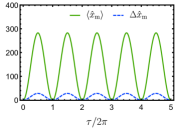
(a)

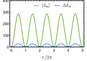
(b)

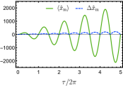
(c)

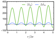
(e)

Figure 5: Plots showing the (dimensionless) expectation value and standard deviation of the mechanical position $\hat{x}_{\mathrm{m}}$ for an initially coherent state of the optics, given (a) undriven evolution, (b) a constant coupling and resonant gravitational field, (c) a time-dependent coupling and time-dependent gravitational field both modulated at resonance, (d) a time-dependent coupling and time-dependent gravitational field both modulated at the fractional frequency $\Omega_{\mathrm{frac}}=4/5$, and finally (e) a time-dependent modulation of the mechanical frequency at parametric resonance. In (d), we note that for this choice of frequency, the system disentangles at $\tau=10\pi$, which we observe as a periodical envelope of the variance and standard deviation. For all cases, the standard deviation $\Delta\hat{x}_{\mathrm{m}}$ remains smaller than $\braket{\hat{x}_{\mathrm{m}}}$. The values $|\mu_{\mathrm{c}}|=10$, $k_{0}=1$, $a=1$, $\epsilon=0.5$, $r_{T}=0$, and the optimal phase choice have been used in all plots.

             

      

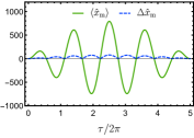
(d)

F.2 Modulated mechanical frequency and time-dependent gravitational field

For the case where the mechanical frequency is being modulated on parametric resonance with $\mathcal{D}_{2}(\tau)=d_{2}\cos(2\tau+\phi_{d2})$ and time dependent gravitational field $\mathcal{D}_{1}(\tau)=-d_{1}(a+\epsilon\cos(\Omega_{d1}\tau+\phi_{d1}))$, we find for the specific case of $\phi_{d1}=0$ and $\phi_{d2}=-\pi/2$,

$$\braket{\hat{x}_{\mathrm{m}}}= 2x_{0}\,\biggl{[}\left(a\,d_{1}+k_{0}\,\braket{\hat{N}_{a}}\right)\left(1-e^{d_{2}\,\tau}\cos(\tau)\right)-\frac{d_{1}\epsilon}{4\,d_{2}}\left(1-e^{-d_{2}\,\tau}\right)\left(d_{2}\,e^{d_{2}\,\tau}\,\cos(\tau)-2\sin(\tau)\right)\biggr{]}\,,$$ (150)

$$(\Delta\hat{x}_{\mathrm{m}})^{2}= \,x_{0}^{2}\Bigg{(}\cosh(2d_{2}\tau)+\sinh(2d_{2}\tau)\cos(2\tau)+4k_{0}^{2}(\Delta\hat{N}_{a})^{2}\left(1-\cos(\tau)e^{d_{2}\tau}\right)^{2}\Bigg{)}$$ (151)

We find that the amplitude of the oscillations increase exponentially due to the parametric driving. Then, the photon number and standard deviation are restricted as $2x_{0}k_{0}\braket{\hat{N}_{a}}(1+e^{d_{2}\tau})\ll l$ and $2x_{0}k_{0}\Delta\hat{N}_{a}(1+e^{d_{2}\tau})\ll l$.

We then plot the expectation value $\braket{\hat{x}_{\mathrm{m}}}$ and the standard deviation $\Delta\hat{x}_{\mathrm{m}}$ as a function of time $\tau$ in Figure 5a. Figure 5a shows $\braket{\hat{x}_{\mathrm{m}}}$ and $\sqrt{\braket{\hat{x}_{\mathrm{m}}^{2}}-\braket{\hat{x}_{\mathrm{m}}}^{2}}$ for undriven evolution, while Figures 5b, 5c, 5d and 5e show the same quantities for resonant gravitational fields, a jointly resonantly modulated coupling and gravitational field, jointly modulated coupling and gravitational field at the fractional frequencies identified in Appendix D, and jointly modulated mechanical frequency and gravitational field, respectively.

Appendix G Phonon number evolution

We saw in the main text that the QFI scales as $\tau^{4}$ when both the gravitational field and the optomechanical coupling is modulated at resonance. Here we investigate what this increase in sensitivity means in terms of the energy stored in the system. Since $\hat{N}_{a}=\hat{a}^{\dagger}\hat{a}$ commutes with the Hamiltonian, the photon number stays constant at all times. The phonon number, however, changes as a result of the optical driving. We here examine how the phonon number changes as a function of time for the same cases as we considered in Appendix F.

When the mechanical element is cooled to the ground state, the phonon number expectation value $\braket{\hat{N}_{b}(\tau)}$ is given by the expression [28]

$$\braket{\hat{N}_{b}(\tau)} =(|\alpha(\tau)|^{2}+(\Gamma^{*}(\tau)\,\Delta(\tau)+\Gamma(\tau)\,\Delta^{*}(\tau))\,\braket{\hat{N}_{a}}+|\Delta(\tau)|^{2}\braket{\hat{N}_{a}^{2}}+|\beta(\tau)|^{2}+|\Gamma(\tau)|^{2}\,,$$ (152)

where $\alpha(\tau)$ and $\beta(\tau)$ are given in (B) and where $\Gamma(\tau)$ and $\Delta(\tau)$ are defined in (F).

We plot the phonon number in Figure 6a according to the same schemes we considered in Appendix 6a. Figure 6a shows $\braket{\hat{N}_{b}}$ of an undriven optomechanical systems with a constant optomechanical coupling, Figure 6b shows $\braket{\hat{N}_{b}}$ for a resonant gravitational field and constant coupling, Figure 6c shows $\braket{\hat{N}_{b}}$ for a doubly resonant gravitational field and coupling, Figure 6d shows $\braket{\hat{N}_{b}}$ for when both the coupling and the gravitational field are modulated at the fractional frequencies, and finally, Figure 6e shows $\braket{\hat{N}_{b}}$ for when the mechanical frequency is modulated at twice the resonant frequency, along with a resonantly modulated gravitational field.

We note from the plots that the phonon number behaves similarly to the position expectation value and variance (see Figure 5a). The phonon number increases monotonically for the doubly-resonant case, but returns to the ground-state once the states disentangle. This occurs, for example, at $\tau=10\pi$ when the fractional frequency is $\Omega_{\mathrm{frac}}=4/5$, as can be seen from Figure 6d. This means that one can achieve a sensitivity that grows linearly in time while at the same time preventing a build-up of energy in the system.

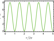
(a)

(b)

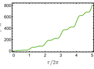
(c)

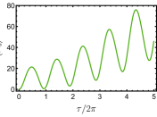
(e)

Figure 6: Plots showing the phonon number $\braket{\hat{N}_{b}}$ for an initially coherent optical state and with the mechanical element in the ground state. The plots show $\braket{\hat{N}_{b}}$ as a function of time for (a) undriven evolution, (b) a constant coupling and resonant gravitational field, (c) a time-dependent coupling and time-dependent gravitational field, both modulated at resonance, (d) a time-dependent coupling and a time-dependent gravitational field, both modulated at the fractional frequency $\Omega_{\mathrm{frac}}=4/5$, and (e) a time-dependent gravitational field at resonance and a modulation of the mechanical frequency at parametric resonance. The values $|\mu_{\mathrm{c}}|=1$, $k_{0}=1$, $a=1$, $\epsilon=0.5$, $r_{T}=0$, and the optimal phase choice $\phi_{d2}=-\pi/2$ have been used in all plots.

             

         

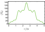
(d)

References

- Abbott et al. [2016] B. P. Abbott, R. Abbott, T. Abbott, M. Abernathy, F. Acernese, K. Ackley, C. Adams, T. Adams, P. Addesso, R. Adhikari, et al., Observation of gravitational waves from a binary black hole merger, Physical Review Letters 116, 061102 (2016).
- Sathyaprakash and Schutz [2009] B. S. Sathyaprakash and B. F. Schutz, Physics, astrophysics and cosmology with gravitational waves, Living Reviews in Relativity 12, 2 (2009).
- Marshall et al. [2003] W. Marshall, C. Simon, R. Penrose, and D. Bouwmeester, Towards Quantum Superpositions of a Mirror, Physical Review Letters 91, 130401 (2003).
- Kleckner et al. [2008] D. Kleckner, I. Pikovski, E. Jeffrey, L. Ament, E. Eliel, J. Van Den Brink, and D. Bouwmeester, Creating and verifying a quantum superposition in a micro-optomechanical system, New Journal of Physics 10, 095020 (2008).
- Derakhshani et al. [2016] M. Derakhshani, C. Anastopoulos, and B. Hu, Probing a gravitational cat state: Experimental possibilities, in Journal of Physics: Conference Series, Vol. 701 (IOP Publishing, 2016) p. 012015.
- Jaffe et al. [2017] M. Jaffe, P. Haslinger, V. Xu, P. Hamilton, A. Upadhye, B. Elder, J. Khoury, and H. Müller, Testing sub-gravitational forces on atoms from a miniature in-vacuum source mass, Nature Physics 13, 938 (2017).
- Bose et al. [2017] S. Bose, A. Mazumdar, G. W. Morley, H. Ulbricht, M. Toroš, M. Paternostro, A. A. Geraci, P. F. Barker, M. S. Kim, and G. Milburn, Spin entanglement witness for quantum gravity, Physical Review Letters 119, 240401 (2017).
- Marletto and Vedral [2017] C. Marletto and V. Vedral, Gravitationally induced entanglement between two massive particles is sufficient evidence of quantum effects in gravity, Physical Review Letters 119, 240402 (2017).
- Wan [2018] C. Wan, Quantum superposition on nano-mechanical oscillator, PhD Thesis (2018).
- Qvarfort et al. [2020] S. Qvarfort, S. Bose, and A. Serafini, Mesoscopic entanglement through central–potential interactions, Journal of Physics B: Atomic, Molecular and Optical Physics 53, 235501 (2020).
- Carlesso et al. [2019] M. Carlesso, A. Bassi, M. Paternostro, and H. Ulbricht, Testing the gravitational field generated by a quantum superposition, New Journal of Physics 21, 093052 (2019).
- Paris [2009] M. G. Paris, Quantum estimation for quantum technology, International Journal of Quantum Information 7, 125 (2009).
- Aasi et al. [2013] J. Aasi, J. Abadie, B. Abbott, R. Abbott, T. Abbott, M. Abernathy, C. Adams, T. Adams, P. Addesso, R. Adhikari, et al., Enhanced sensitivity of the LIGO gravitational wave detector by using squeezed states of light, Nature Photonics 7, 613 (2013).
- Aspelmeyer et al. [2014] M. Aspelmeyer, T. J. Kippenberg, and F. Marquardt, Cavity optomechanics, Review of Modern Physics 86 (2014).
- Favero and Karrai [2009] I. Favero and K. Karrai, Optomechanics of deformable optical cavities, Nature Photonics 3, 201 (2009).
- Millen et al. [2020] J. Millen, T. S. Monteiro, R. Pettit, and A. N. Vamivakas, Optomechanics with levitated particles, Reports on Progress in Physics 83, 026401 (2020).
- Bahl et al. [2013] G. Bahl, K. H. Kim, W. Lee, J. Liu, X. Fan, and T. Carmon, Brillouin cavity optomechanics with microfluidic devices, Nature Communications 4, 1 (2013).
- Kashkanova et al. [2017] A. Kashkanova, A. Shkarin, C. Brown, N. Flowers-Jacobs, L. Childress, S. Hoch, L. Hohmann, K. Ott, J. Reichel, and J. Harris, Superfluid brillouin optomechanics, Nature Physics 13, 74 (2017).
- Enzian et al. [2019] G. Enzian, M. Szczykulska, J. Silver, L. Del Bino, S. Zhang, I. A. Walmsley, P. Del’Haye, and M. R. Vanner, Observation of brillouin optomechanical strong coupling with an 11 ghz mechanical mode, Optica 6, 7 (2019).
- Kuhn et al. [2017] S. Kuhn, B. A. Stickler, A. Kosloff, F. Patolsky, K. Hornberger, M. Arndt, and J. Millen, Optically driven ultra-stable nanomechanical rotor, Nature Communications 8, 1 (2017).
- Schliesser and Kippenberg [2010] A. Schliesser and T. J. Kippenberg, Cavity optomechanics with whispering-gallery mode optical micro-resonators, in Advances In Atomic, Molecular, and Optical Physics, Vol. 58 (Elsevier, 2010) pp. 207–323.
- Li and Barker [2018] Y. L. Li and P. Barker, Characterization and testing of a micro-g whispering gallery mode optomechanical accelerometer, Journal of Lightwave Technology 36, 3919 (2018).
- Singh et al. [2014] V. Singh, S. Bosman, B. Schneider, Y. M. Blanter, A. Castellanos-Gomez, and G. Steele, Optomechanical coupling between a multilayer graphene mechanical resonator and a superconducting microwave cavity, Nature Nanotechnology 9, 820 (2014).
- Delić et al. [2020] U. Delić, M. Reisenbauer, K. Dare, D. Grass, V. Vuletić, N. Kiesel, and M. Aspelmeyer, Cooling of a levitated nanoparticle to the motional quantum ground state, Science 367, 892 (2020).
- Qvarfort et al. [2018] S. Qvarfort, A. Serafini, P. F. Barker, and S. Bose, Gravimetry through non-linear optomechanics, Nature Communications 9, 3690 (2018).
- Armata et al. [2017] F. Armata, L. Latmiral, A. Plato, and M. Kim, Quantum limits to gravity estimation with optomechanics, Physical Review A 96, 043824 (2017).
- Bruschi and Xuereb [2018] D. E. Bruschi and A. Xuereb, ‘mechano-optics’: An optomechanical quantum simulator, New Journal of Physics 20, 065004 (2018).
- Qvarfort et al. [2019a] S. Qvarfort, A. Serafini, A. Xuereb, D. Braun, D. Rätzel, and D. E. Bruschi, Time-evolution of nonlinear optomechanical systems: Interplay of mechanical squeezing and non-Gaussianity, Journal of Physics A: Mathematical and Theoretical (2019a).
- Schneiter et al. [2020] F. Schneiter, S. Qvarfort, A. Serafini, A. Xuereb, D. Braun, D. Rätzel, and D. E. Bruschi, Optimal estimation with quantum optomechanical systems in the nonlinear regime, Physical Review A 101, 033834 (2020).
- Liao et al. [2014] J.-Q. Liao, K. Jacobs, F. Nori, and R. W. Simmonds, Modulated electromechanics: large enhancements of nonlinearities, New Journal of Physics 16, 072001 (2014).
- Yin et al. [2017] T.-S. Yin, X.-Y. Lü, L.-L. Zheng, M. Wang, S. Li, and Y. Wu, Nonlinear effects in modulated quantum optomechanics, Physical Review A 95, 053861 (2017).
- Szorkovszky et al. [2011] A. Szorkovszky, A. C. Doherty, G. I. Harris, and W. P. Bowen, Mechanical squeezing via parametric amplification and weak measurement, Physical review letters 107, 213603 (2011).
- Millen et al. [2015] J. Millen, P. Z. G. Fonseca, T. Mavrogordatos, T. S. Monteiro, and P. F. Barker, Cavity cooling a single charged levitated nanosphere, Physical Review Letters 114, 123602 (2015).
- Fonseca et al. [2016] P. Z. G. Fonseca, E. B. Aranas, J. Millen, T. S. Monteiro, and P. F. Barker, Nonlinear dynamics and strong cavity cooling of levitated nanoparticles, Physical Review Letters 117, 173602 (2016).
- Aranas et al. [2016] E. B. Aranas, P. Z. G. Fonseca, P. F. Barker, and T. S. Monteiro, Split-sideband spectroscopy in slowly modulated optomechanics, New Journal of Physics 18, 113021 (2016).
- Levitan et al. [2016] B. A. Levitan, A. Metelmann, and A. A. Clerk, Optomechanics with two-phonon driving, New Journal of Physics 18, 093014 (2016).
- Rätzel and Fuentes [2019] D. Rätzel and I. Fuentes, Testing small scale gravitational wave detectors with dynamical mass distributions, Journal of Physics Communications 3, 025009 (2019), arXiv:1709.08099 [gr-qc] .
- Law [1995] C. Law, Interaction between a moving mirror and radiation pressure: A hamiltonian formulation, Physical Review A 51, 2537 (1995).
- Chang et al. [2010] D. E. Chang, C. A. Regal, S. B. Papp, D. J. Wilson, J. Ye, O. Painter, H. J. Kimble, and P. Zoller, Cavity opto-mechanics using an optically levitated nanosphere, Proceedings of the National Academy of Sciences 107, 1005 (2010).
- Rugar and Grütter [1991] D. Rugar and P. Grütter, Mechanical parametric amplification and thermomechanical noise squeezing, Physical Review Letters 67, 699 (1991).
- Aranas et al. [2017] E. Aranas, P. Fonseca, P. Barker, and T. Monteiro, Thermometry of levitated nanoparticles in a hybrid electro-optical trap, Journal of Optics 19, 034003 (2017).
- Qvarfort et al. [2019b] S. Qvarfort, A. Serafini, A. Xuereb, D. Rätzel, and D. E. Bruschi, Enhanced continuous generation of non-Gaussianity through optomechanical modulation, New Journal of Physics 21, 055004 (2019b).
- Wei and Norman [1963] J. Wei and E. Norman, Lie algebraic solution of linear differential equations, Journal of Mathematical Physics 4, 575 (1963).
- Wolf and Korsch [1988] F. Wolf and H. Korsch, Time-evolution operators for (coupled) time-dependent oscillators and lie algebraic structure theory, Physical Review A 37, 1934 (1988).
- Choi and Nahm [2007] J. Choi and I. Nahm, Su (1, 1) lie algebra applied to the general time-dependent quadratic hamiltonian system, International Journal of Theoretical Physics 46, 1 (2007).
- Bruschi et al. [2013] D. E. Bruschi, A. R. Lee, and I. Fuentes, Time evolution techniques for detectors in relativistic quantum information, Journal of Physics A: Mathematical and Theoretical 46, 165303 (2013).
- Teuber and Scheel [2020] L. Teuber and S. Scheel, Solving the quantum master equation of coupled harmonic oscillators with lie-algebra methods, Physical Review A 101, 042124 (2020).
- Park and Wang [2009] Y.-S. Park and H. Wang, Resolved-sideband and cryogenic cooling of an optomechanical resonator, Nature physics 5, 489 (2009).
- Chan et al. [2011] J. Chan, T. M. Alegre, A. H. Safavi-Naeini, J. T. Hill, A. Krause, S. Gröblacher, M. Aspelmeyer, and O. Painter, Laser cooling of a nanomechanical oscillator into its quantum ground state, Nature 478, 89 (2011).
- Teufel et al. [2011] J. D. Teufel, T. Donner, D. Li, J. W. Harlow, M. Allman, K. Cicak, A. J. Sirois, J. D. Whittaker, K. W. Lehnert, and R. W. Simmonds, Sideband cooling of micromechanical motion to the quantum ground state, Nature 475, 359 (2011).
- Wu et al. [1986] L.-A. Wu, H. Kimble, J. Hall, and H. Wu, Generation of squeezed states by parametric down conversion, Physical Review Letters 57, 2520 (1986).
- Slusher et al. [1985] R. Slusher, L. Hollberg, B. Yurke, J. Mertz, and J. Valley, Observation of squeezed states generated by four-wave mixing in an optical cavity, Physical Review Letters 55, 2409 (1985).
- Eberle et al. [2010] T. Eberle, S. Steinlechner, J. Bauchrowitz, V. Händchen, H. Vahlbruch, M. Mehmet, H. Müller-Ebhardt, and R. Schnabel, Quantum enhancement of the zero-area sagnac interferometer topology for gravitational wave detection, Physical Review Letters 104, 251102 (2010).
- Mehmet et al. [2011] M. Mehmet, S. Ast, T. Eberle, S. Steinlechner, H. Vahlbruch, and R. Schnabel, Squeezed light at 1550 nm with a quantum noise reduction of 12.3 db, Optics Express 19, 25763 (2011).
- Vahlbruch et al. [2016] H. Vahlbruch, M. Mehmet, K. Danzmann, and R. Schnabel, Detection of 15 db squeezed states of light and their application for the absolute calibration of photoelectric quantum efficiency, Physical Review Letters 117, 110801 (2016).
- Adesso et al. [2009] G. Adesso, F. Dell’Anno, S. De Siena, F. Illuminati, and L. Souza, Optimal estimation of losses at the ultimate quantum limit with non-gaussian states, Physical Review A 79, 040305 (2009).
- Benatti and Braun [2013] F. Benatti and D. Braun, Sub–shot-noise sensitivities without entanglement, Physical Review A 87, 012340 (2013).
- Tiedau et al. [2019] J. Tiedau, T. J. Bartley, G. Harder, A. E. Lita, S. W. Nam, T. Gerrits, and C. Silberhorn, Scalability of parametric down-conversion for generating higher-order fock states, Physical Review A 100, 041802 (2019).
- Braunstein and Caves [1994] S. L. Braunstein and C. M. Caves, Statistical distance and the geometry of quantum states, Physical Review Letters 72, 3439 (1994).
- Pang and Brun [2014] S. Pang and T. A. Brun, Quantum metrology for a general Hamiltonian parameter, Physical Review A 90, 022117 (2014).
- Jing et al. [2014] L. Jing, J. Xiao-Xing, Z. Wei, and W. Xiao-Guang, Quantum fisher information for density matrices with arbitrary ranks, Communications in Theoretical Physics 61, 45 (2014).
- Bose et al. [1997] S. Bose, K. Jacobs, and P. Knight, Preparation of nonclassical states in cavities with a moving mirror, Physical Review A 56, 4175 (1997).
- Szorkovszky et al. [2013] A. Szorkovszky, G. A. Brawley, A. C. Doherty, and W. P. Bowen, Strong thermomechanical squeezing via weak measurement, Physical Review Letters 110, 184301 (2013).
- Bothner et al. [2020] D. Bothner, S. Yanai, A. Iniguez-Rabago, M. Yuan, Y. M. Blanter, and G. A. Steele, Cavity electromechanics with parametric mechanical driving, Nature Communications 11, 1 (2020).
- Weedbrook et al. [2012] C. Weedbrook, S. Pirandola, R. García-Patrón, N. J. Cerf, T. C. Ralph, J. H. Shapiro, and S. Lloyd, Gaussian quantum information, Reviews of Modern Physics 84, 621 (2012).
- Schnabel [2017] R. Schnabel, Squeezed states of light and their applications in laser interferometers, Physics Reports 684, 1 (2017).
- Ast et al. [2013] S. Ast, M. Mehmet, and R. Schnabel, High-bandwidth squeezed light at 1550 nm from a compact monolithic ppktp cavity, Optics Express 21, 13572 (2013).
- Bruschi and Wilhelm [2020] D. E. Bruschi and F. K. Wilhelm, Self gravity affects quantum states, arXiv preprint arXiv:2006.11768 (2020).
- Schmöle et al. [2016] J. Schmöle, M. Dragosits, H. Hepach, and M. Aspelmeyer, A micromechanical proof-of-principle experiment for measuring the gravitational force of milligram masses, Classical and Quantum Gravity 33, 125031 (2016).
- Singh et al. [2017] S. Singh, L. De Lorenzo, I. Pikovski, and K. Schwab, Detecting continuous gravitational waves with superfluid 4he, New Journal of Physics 19, 073023 (2017).
- Sabín et al. [2014] C. Sabín, D. E. Bruschi, M. Ahmadi, and I. Fuentes, Phonon creation by gravitational waves, New Journal of Physics 16, 085003 (2014).
- Marshman et al. [2020] R. J. Marshman, A. Mazumdar, G. Morley, P. F. Barker, S. Hoekstra, and S. Bose, Mesoscopic interference for metric and curvature (mimac) & gravitational wave detection, New Journal of Physics 22, 083012 (2020).
- Arvanitaki and Geraci [2013] A. Arvanitaki and A. A. Geraci, Detecting high-frequency gravitational waves with optically levitated sensors, Physical Review Letters 110, 071105 (2013).
- Maggiore [2008] M. Maggiore, Gravitational Waves: Volume 1: Theory and Experiments, Vol. 1 (Oxford university press, 2008).
- Rätzel et al. [2018] D. Rätzel, F. Schneiter, D. Braun, T. Bravo, R. Howl, M. P. E. Lock, and I. Fuentes, Frequency spectrum of an optical resonator in a curved spacetime, New Journal of Physics 20, 053046 (2018).
- Moore et al. [2014] C. J. Moore, R. H. Cole, and C. P. L. Berry, Gravitational-wave sensitivity curves, Classical and Quantum Gravity 32, 015014 (2014).
- Sesana [2016] A. Sesana, Prospects for multiband gravitational-wave astronomy after gw150914, Physícal Review Letters 116, 231102 (2016).
- Hsu et al. [2016] J.-F. Hsu, P. Ji, C. W. Lewandowski, and B. D’Urso, Cooling the motion of diamond nanocrystals in a magneto-gravitational trap in high vacuum, Scientific reports 6, 30125 (2016).
- Cirio et al. [2012] M. Cirio, G. K. Brennen, and J. Twamley, Quantum magnetomechanics: Ultrahigh--levitated mechanical oscillators, Physical Review Letters 109, 147206 (2012).
- O’Brien et al. [2019] M. O’Brien, S. Dunn, J. Downes, and J. Twamley, Magneto-mechanical trapping of micro-diamonds at low pressures, Applied Physics Letters 114, 053103 (2019).
- Johnsson et al. [2016] M. T. Johnsson, G. K. Brennen, and J. Twamley, Macroscopic superpositions and gravimetry with quantum magnetomechanics, Scientific reports 6, 37495 (2016).
- Bullier et al. [2019] N. Bullier, A. Pontin, and P. Barker, Super-resolution imaging of a low frequency levitated oscillator, Review of Scientific Instruments 90, 093201 (2019).
- Arcizet et al. [2006] O. Arcizet, P.-F. Cohadon, T. Briant, M. Pinard, and A. Heidmann, Radiation-pressure cooling and optomechanical instability of a micromirror, Nature 444, 71 (2006).
- Romero-Isart et al. [2011] O. Romero-Isart, A. C. Pflanzer, M. L. Juan, R. Quidant, N. Kiesel, M. Aspelmeyer, and J. I. Cirac, Optically levitating dielectrics in the quantum regime: Theory and protocols, Physical Review A 83, 013803 (2011).
- Serafini [2017] A. Serafini, Quantum Continuous Variables: A Primer of Theoretical Methods (CRC Press, 2017).
- Bruschi [2020] D. E. Bruschi, Time evolution of two harmonic oscillators with cross-Kerr interactions, Journal of Mathematical Physics 61, 032102 (2020).
- Casimir and Polder [1948] H. Casimir and D. Polder, The influence of retardation on the London-van der Waals forces, Physical Review 73, 360 (1948).
- Bimonte [2017] G. Bimonte, Going beyond pfa: A precise formula for the sphere-plate Casimir force, EPL (Europhysics Letters) 118, 20002 (2017).
- Rodriguez-Lopez [2011] P. Rodriguez-Lopez, Casimir energy and entropy in the sphere-sphere geometry, Physical Review B 84, 075431 (2011).
- Chiaverini et al. [2003] J. Chiaverini, S. Smullin, A. Geraci, D. Weld, and A. Kapitulnik, New experimental constraints on non-newtonian forces below 100 m, Physical Review Letters 90, 151101 (2003).
- Munday et al. [2009] J. N. Munday, F. Capasso, and V. A. Parsegian, Measured long-range repulsive Casimir–Lifshitz forces, Nature 457, 170 (2009).
- Intravaia et al. [2013] F. Intravaia, S. Koev, I. W. Jung, A. A. Talin, P. S. Davids, R. S. Decca, V. A. Aksyuk, D. A. Dalvit, and D. López, Strong Casimir force reduction through metallic surface nanostructuring, Nature Communications 4, 1 (2013).
- Banishev et al. [2012] A. A. Banishev, C.-C. Chang, R. Zandi, and U. Mohideen, Modulation and cancellation of the Casimir force by using radiation pressure, Applied Physics Letters 100, 033112 (2012), publisher: American Institute of Physics.
- Chen et al. [2007] F. Chen, G. L. Klimchitskaya, V. M. Mostepanenko, and U. Mohideen, Control of the Casimir force by the modification of dielectric properties with light, Physical Review B 76, 035338 (2007), publisher: American Physical Society.
- Leonhardt and Philbin [2007] U. Leonhardt and T. G. Philbin, Quantum levitation by left-handed metamaterials, New Journal of Physics 9, 254 (2007).
- Brune et al. [1990] M. Brune, S. Haroche, V. Lefevre, J. M. Raimond, and N. Zagury, Quantum nondemolition measurement of small photon numbers by Rydberg-atom phase-sensitive detection, Physical Review Letters 65, 976 (1990).
- Fujiwara [2001] A. Fujiwara, Quantum channel identification problem, Physical Review A 63, 042304 (2001).
- Giovannetti et al. [2006] V. Giovannetti, S. Lloyd, and L. Maccone, Quantum metrology, Physical Review Letters 96, 010401 (2006).
- Tufarelli et al. [2014] T. Tufarelli, A. Ferraro, A. Serafini, S. Bose, and M. S. Kim, Coherently opening a high-q cavity, Physical Review Letters 112, 133605 (2014).
- Flayac and Savona [2013] H. Flayac and V. Savona, Input-output theory of the unconventional photon blockade, Physical Review A 88, 033836 (2013).
- Zhang et al. [2014] J. Zhang, Y.-x. Liu, R.-B. Wu, K. Jacobs, S. K. Ozdemir, L. Yang, T.-J. Tarn, and F. Nori, Nonlinear quantum input-output analysis using volterra series, arXiv preprint arXiv:1407.8108 (2014).
- Caneva et al. [2015] T. Caneva, M. T. Manzoni, T. Shi, J. S. Douglas, J. I. Cirac, and D. E. Chang, Quantum dynamics of propagating photons with strong interactions: a generalized input–output formalism, New Journal of Physics 17, 113001 (2015).
- Combes et al. [2017] J. Combes, J. Kerckhoff, and M. Sarovar, The slh framework for modeling quantum input-output networks, Advances in Physics: X 2, 784 (2017).
- Wei and Norman [1964] J. Wei and E. Norman, On global representations of the solutions of linear differential equations as a product of exponentials, Proceedings of the American Mathematical Society 15, 327 (1964).
- Kovacic et al. [2018] I. Kovacic, R. Rand, and S. M. Sah, Mathieu’s equation and its generalizations: Overview of stability charts and their features, Applied Mechanics Reviews 70, 020802 (2018).
- Yuen [1976] H. P. Yuen, Two-photon coherent states of the radiation field, Physical Review A 13, 2226 (1976).
- Braun [2011] D. Braun, Ultimate quantum bounds on mass measurements with a nano-mechanical resonator, Europhysics Letters 94, 68007 (2011).