Fast computation of spherical phase-space functions of quantum many-body states

Abstract

Quantum devices are preparing increasingly more complex entangled quantum states. How can one effectively study these states in light of their increasing dimensions? Phase spaces such as Wigner functions provide a suitable framework. We focus on phase spaces for finite-dimensional quantum states of single qudits or permutationally symmetric states of multiple qubits. We present methods to efficiently compute the corresponding phase-space functions which are at least an order of magnitude faster than traditional methods. Quantum many-body states in much larger dimensions can now be effectively studied by experimentalist and theorists using these phase-space techniques.

I Introduction

Current (and near-term) quantum devices are expected to prepare increasingly more complex entangled quantum states Arute et al. (2019); Omran et al. (2019); Song et al. (2019); Preskill (2018). How can one effectively illustrate and analyze these states in light of their increasing dimensions? Phase spaces Schleich (2001); Zachos et al. (2005); Schroeck (2013); Curtright et al. (2014) such as Wigner functions have been widely used to meet this challenge. We will focus in this work on representing (finite-dimensional) quantum states of single qudits or permutationally symmetric states of multiple qubits using spherical phase spaces Koczor et al. (2020); Koczor (2019).

Permutationally symmetric states include, e.g., Greenberger–Horne–Zeilinger (GHZ) and squeezed states, and they have immediate applications in quantum metrology for optimally estimating, e.g., magnetic field strengths Pezzè et al. (2018); Tóth and Apellaniz (2014); Giovannetti et al. (2011); Koczor et al. (shed). Phase spaces are a useful tool for visualizing experimentally generated quantum many-body states of atomic ensembles Arute et al. (2019); Omran et al. (2019); McConnell et al. (2015); Haas et al. (2014), Bose-Einstein condensates Anderson et al. (1995); Ho (1998); Ohmi and Machida (1998); Stenger et al. (1998); Lin et al. (2011); Riedel et al. (2010); Schmied and Treutlein (2011); Hamley et al. (2012); Strobel et al. (2014), trapped ions Leibfried et al. (2005); Bohnet et al. (2016); Monz et al. (2011), and light polarization Bouchard et al. (2017); Klimov et al. (2017); Chaturvedi et al. (2006). On the theoretical side, phase spaces provide the necessary intuition as they naturally reduce to classical phase spaces in the limit of a vanishing Planck constant Groenewold (1946); Moyal (1949); Bayen et al. (1978a, b); Berezin (1974, 1975). Such phase-space techniques, and related quantization methods Weyl (1927, 1931, 1950), also play a vital role in harmonic analysis and in the theory of pseudo-differential operators de Gosson (2017, 2016); Gröchenig (2001); Cohen (1966, 1995).

Figure 1: (a) Run times of earlier Methods A and B relative to our Method C for computing phase-space functions of quantum states with an increasing dimension $d=2J{+}1$ are at least an order of magnitude slower. Methods A and B both employ tensor-operator decompositions (Sec. III). Method A relies on Mathematica’s built-in method to compute Clebsch-Gordan coefficients and Method B uses an efficient, recursive algorithm Schulten and Gordon (1976, 1975); Luscombe and Luban (1998); Dumont (2018). Our Method C (Sec. V) combines spherical sampling techniques Driscoll and Healy (1994); Kennedy and Sadeghi (2013), explicit descriptions of rotation operators Tajima (2015); Feng et al. (2015), Fourier series expansions, and fast Fourier transforms (FFT). The run times depend only on $d$ and not the quantum state. (b) Root mean square (RMS) errors for certain quantum states Note (1) relative to their analytically known formula. Method C shows a high numerical precision comparable to machine precision.

In this work, we consider spherical phase spaces of finite-dimensional quantum states and we develop a novel approach to efficiently compute these phase-space representations. For up to which dimensions can phase spaces be practically utilized? Our approach has a significant advantage in this regard as it allows for much larger dimensions to be addressed in a reasonable time frame. Therefore, phase-space descriptions of quantum many-body states are now feasible for dimensions which were beyond the reach of prior approaches. In summary, our results will enable practitioners and experimentalist—but also theorists—to visualise and study complex quantum states in considerably larger dimensions.

This is accomplished by applying an efficiently computable Fourier series expansion and a fast Fourier transform (FFT) Allen and Mills (2004). In particular, Fig. 1(a) compares the the run time of our Method C (as detailed in Sec. V) to the traditional Methods A and B (see Sec. III) and, indeed, our Method C is at least an order of magnitude faster. Moreover, Fig. 1(b) highlights that the root-mean-square error of certain test cases is comparable to machine precision for the considered dimensions and this suggests that our approach is numerically stable. We provide implementations in various programming environments (see Sec. V.4 and Koczor (2020)), including C Kernighan and Ritchie (1988), MATLAB The MathWorks Inc. , Mathematica Wolfram Research, Inc. , and Python Van Rossum and Drake Jr (1995).

Our work has the following structure: We first discuss our motivation and highlight applications in Sec. II. Prior computational approaches to determine phase-space representations of finite-dimensional quantum systems are considered in Sec. III. In order to set the stage, we shortly recall the parity-operator description of spherical phase spaces which we have developed in Koczor et al. (2020). Section V constitutes the main part of our manuscript where we develop our novel approach to efficiently compute spherical phase-space representations up to arbitrarily fine resolutions. We continue with a discussion of our results and further applications in Sec. VI, before we conclude. Important details are explained in appendices.

II Motivation and Applications

Various quantum-technology efforts (such as quantum computing or metrology) aim at creating large entangled multi-qubit states. Here, we focus in particular on the important class of states that are symmetric under permutations of qubits. These states include important families such as GHZ or squeezed states which are central in, e.g., quantum metrology Pezzè et al. (2018) or entanglement verification Omran et al. (2019); Song et al. (2019). They are also typically illustrated and analyzed in their phase-space representation (see, e.g., Song et al. (2019); Pezzè et al. (2018)) which can be naturally plotted on the surface of a sphere. This is reflected by the inherent symmetries and reduced degrees of freedom as compared to general multi-qubit states. Before starting the technical discussion in Sec. III, we will now motivate our topic and highlight applications.

We first recall that permutationally symmetric states with $N=2J$ qubits can be mapped to states of a single spin $J$ (or qudit with $d=2J{+}1$) where $J$ denotes a positiv integer or half-integer Koczor et al. (2019a); Koczor (2019); Dicke (1954); Stockton et al. (2003); Tóth et al. (2010); Lücke et al. (2014). Permutation symmetry appears in various applications including probe states in quantum metrology for optimal sensing, e.g., magnetic fields Pezzè et al. (2018); Tóth and Apellaniz (2014); Giovannetti et al. (2011); Koczor et al. (shed). Permutationally symmetric qubit states can be efficiently reconstructed and are used for entanglement verification Tóth et al. (2010); Stockton et al. (2003); Lücke et al. (2014); Pezzè et al. (2018); Omran et al. (2019); Song et al. (2019). We will illustrate a few practically relevant, high-dimensional examples for which traditional methods (see Sec. III) take an impractically large amount of time in order to determine the desired phase-space function. Further discussions and applications are deferred to Sec. VI.

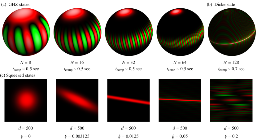
Figure 2: Applications highlighted by numerically computed Wigner functions of single-qudit states with $d=2J{+}1$ which are equivalent to permutation-symmetric states of $N=d{-}1$ qubits: (a) GHZ states for $N\in\{8,16,32,64\}$, (b) Dicke state $|Jm\rangle$ for $N=128$ and $m=0$. The run time (without 3D graphics and rasterization) using Method D (Sec. V) on a laptop in Mathematica is dominated by the FFT on a $1024\times 1024$ grid. (c) Similarly, Wigner functions of squeezed states $|\xi\rangle:=\exp[-i\xi\,\mathcal{I}_{x}^{2}]|0\rangle^{\otimes N}$ with varying squeezing angle $\xi$ and fixed $d=N{+}1=500$ in a plane for a small spherical subset with $|\theta|\leq 0.05\pi$ (run time $\approx 1$ min): Gaussian for $\xi=0$ (left); squeezed Gaussians for $\xi<0.05$. Larger $\xi\geq 0.05$ lead to non-trivial and rapidly oscillating shapes which are nicely recovered, while analytical approximations fail in this regime. Red (dark gray) and green (light gray) for positive and negative values, respectively. The brightness indicates the absolute value of the function relative to its global maximum.

The first example considers and highlights the Greenberger–Horne–Zeilinger (GHZ) state $(|0\rangle^{\otimes N}+|1\rangle^{\otimes N})/\sqrt{2}$ as the superposition of the all-zero and all-one state for $N$ qubits which can be interpreted as the spin-up and spin-down states of a single qudit. Their high degree of entanglement supports the ultimate quantum precision in metrology, which is known as the Heisenberg limit Pezzè et al. (2018). GHZ states have been successfully created in numerous experiments with, e.g., trapped ions Monz et al. (2011), superconducting qubits Song et al. (2019), and Rydberg atoms Omran et al. (2019) for up to 20 qubits. Although phase-space functions of GHZ states can be analytically approximated for large dimensions Koczor et al. (2020, 2019a), we are interested in computing them exactly within numerical precision and without relying on approximations. Figure 2(a) shows Wigner functions of GHZ states for an increasing number of qubits with $N\in\{8,16,32,64\}$. Already the case $N=32$ is currently beyond the experimental state of the art Omran et al. (2019); Song et al. (2019), but near-term quantum hardware are expected to deliver GHZ states of larger dimensions via, e.g., linear-depth quantum circuits Preskill (2018).

We also consider so-called symmetric Dicke states Dicke (1954) which are defined Koczor (2019); Stockton et al. (2003) as a superposition of all permutations of computational basis states with a fixed number of zeros and ones in a multi-qubit system. In particular,

$$|Nn\rangle:=\tfrac{1}{\sqrt{p}}\,\sum_{k=1}^{p}P_{k}\,|\underbrace{1,1,\dots,1}_{n},\underbrace{0,\dots,0}_{N-n}\rangle,$$ (1)

where the sum runs over all $p=\binom{N}{n}$ distinct permutations $P_{k}$ of the $N$ qubits. These states are isomorphic to the single-qudit states $|Jm\rangle$ by mapping $N$ to $J/2$ and $m$ to $(N/2-n)$. We plot the Dicke state $|Jm\rangle$ with $d=2J{+}1=129$ and $m=0$ in Fig. 2(b). This corresponds to a highly entangled quantum state of 128 indistinguishable qubits where 64 qubits are in the $|0\rangle$ state and 64 qubits are in the $|1\rangle$ state (refer to Eq. (1)). One observes an axial symmetry (i.e. invariance under global $Z$ rotations) and strong entanglement results in heavily oscillating Wigner functions in Fig. 2(b).

Finally, squeezed states $|\xi\rangle:=\exp[-i\xi\,\mathcal{I}_{x}^{2}]|0\rangle^{\otimes N}$ are obtained from the spin-up state of a single qudit or, equivalently, the all-zero state of $N$ qubits under the influence of a squeezing interaction Hamiltonian $\mathcal{I}_{x}^{2}$. The corresponding evolution time $\xi$ is known as the squeezing angle Ma et al. (2011) and $\mathcal{I}_{x}$ is the $x$ component of the total angular momentum operator, i.e., proportional to the sum of all Pauli $\sigma_{x}$ operators that act on different qubits. These states have been created in various experiments including Bose-Einstein condensates Anderson et al. (1995); Ho (1998); Ohmi and Machida (1998); Stenger et al. (1998); Lin et al. (2011); Riedel et al. (2010); Schmied and Treutlein (2011); Hamley et al. (2012); Strobel et al. (2014); Hosten et al. (2016) for up to thousands of atoms. In such experiments, these finite-dimensional squeezed states correspond to internal degrees of freedom (which we treat as an effective qudit) of fundamentally indistinguishable atoms. We plot their Wigner functions for the case of $d=N+1=500$ and an increasing squeezing angle $\xi$ in Fig. 2(c). For such large dimensions squeezed states with small squeezing angles can be approximated well using the techniques described in Koczor et al. (2020, 2019a). In particular, the spin-up state $|0\rangle^{\otimes N}$ for $\xi=0$ in Fig. 2(c) is a Gaussian-like function because the sphere can be approximated locally as a plane. For small squeezing angles, these states can be analytically approximated using star products Koczor et al. (2019a); Klimov and Espinoza (2005). Their phase-space representations are squeezed Gaussian functions which are very similar to the ones known in quantum optics Ma et al. (2011); Leonhardt (1997). This is illustrated in Fig. 2(c) where the aforementioned approximations apply to the cases $\xi=0$, $\xi=0.003125$, and $\xi=0.0125$. For larger squeezing angles, Wigner functions will, however, deviate strongly from simple squeezed Gaussian states and non-trivial, heavily oscillating contributions become dominant as is shown in Fig. 2(c) for $\xi=0.05$ and $\xi=0.2$. This motivates our numerical approach to exactly determine phase-space functions for large spin-like systems (and permutationally symmetric multi-qubit states) where analytical approximations do usually fail.

III Traditional methods to compute spherical phase-space functions

We now discuss traditional methods to compute phase-space functions of qudit states with $d=2J{+}1$ and consider the full class of $s$-parametrized phase spaces with $-1\leq s\leq 1$. This includes Wigner functions ($s=0$) Dowling et al. (1994), Husimi $Q$ functions ($s=-1$) Agarwal (1981), and Glauber $P$ functions ($s=1$). Spherical phase spaces are parametrized by two Euler angles $(\theta,\phi)$ with $0\leq\theta\leq\pi$ and $0\leq\phi<2\pi$. Building on the pioneering work by Agarwal Agarwal (1981); Dowling et al. (1994), $s$-parametrized phase-space functions Koczor et al. (2020)

$$F_{\rho}(\theta,\phi,s)=\tfrac{1}{R}\,\sum_{j=0}^{2J}\sum_{m=-j}^{j}(\gamma_{j})^{-s}\,c_{jm}\,\mathrm{Y}_{jm}(\theta,\phi)$$ (2)

can be expanded into spherical harmonics $\mathrm{Y}_{jm}(\theta,\phi)$ Jackson (1999). The constant $\gamma_{j}:=R\,\sqrt{4\pi}(2J)!\,[(2J{+}j{+}1)!\,(2J{-}j)!\,]^{{-}1/2}$ and the spherical radius $R:=\sqrt{J/(2\pi)}$ are used in Eq. (2). The expansion coefficients $c_{jm}:=\mathrm{Tr}\,[\rho\,\mathrm{T}_{jm}^{\dagger}]$ are computed from the density matrix $\rho$ and the tensor-operator coefficients $\mathrm{T}_{jm}$ Racah (1942); Fano and Racah (1959); Silver (1976); Chaichian and Hagedorn (1998). The matrix elements

$$[\mathrm{T}_{jm}]_{m_{1}m_{2}} =\sqrt{(2j{+}1)/(2J{+}1)}\,C^{Jm_{1}}_{Jm_{2},jm}$$ (3a)

$$=(-1)^{J-m_{2}}\,C^{jm}_{Jm_{1},J,-m_{2}}$$ (3b)

are determined by Clebsch-Gordan coefficients $C^{Jm_{1}}_{Jm_{2},jm}$ where $m_{1},m_{2}\in\{J,\ldots,-J\}$ Messiah (1962); Brif and Mann (1999, 1997); Biedenharn and Louck (1981); Fano (1953).

Equation (2) describes the standard approach for numerically computing spherical phase-space functions. In a first step, it relies on efficient approaches to calculate Clebsch-Gordan coefficients. The calculation of the expansion coefficients $c_{jm}$ is, however, computationally expensive for large dimensions $d=2J{+}1\gg 1$. In particular, one needs to determine $\mathcal{O}(d^{2})$ distinct tensor-operators $\mathrm{T}_{jm}$ and their matrix entries. Appendix A clarifies that $\mathcal{O}(d^{3})$ Clebsch-Gordan coefficients have to be calculated which dominates the run time for computing all of the $\mathcal{O}(d^{2})$ expansion coefficients $c_{jm}$ in Eq. (2).

Two different approaches to calculate Clebsch-Gordan coefficients result in two different methods (Method A and B) to the coefficients $c_{jm}$. Method A uses the built-in Mathematica Wolfram Research, Inc. function that performs arbitrary-precision integer arithmetic. In Method B, the run time can be significantly reduced by numerically computing Clebsch-Gordan coefficients using a FORTRAN Backus and Heising (1964) implementation Dumont (2018) of a recursive algorithm Schulten and Gordon (1976, 1975); Luscombe and Luban (1998). Methods A and B are compared in Fig. (3). For Method A (B), all tensor operators for certain dimensions $d\leq 300$ ($d\leq 500$) have been determined and we estimate a complexity $\mathcal{O}(d^{4})$ in this range.

After the expansion coefficients $c_{jm}$ have been obtained, the phase-space function $F_{\rho}(\theta,\phi,s)$ is spherically sampled in a second step by applying a fast spherical harmonics transform which might rely on equiangular samples or Gauss-Legendre grids. The second step requires a practically and asymptotically negligible time of $\mathcal{O}(d^{3})$ when compared to the first step. Spherical harmonics transforms are widely used in various scientific contexts and efficient implementations are available Suda and Takami (2002); Driscoll and Healy (1994); Reinecke, M. and Seljebotn, D. S. (2013); Schaeffer (2013); Mohlenkamp (1999).

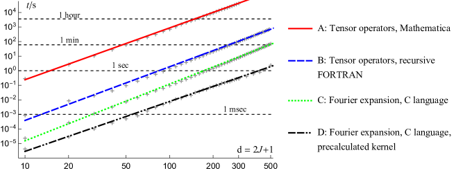
Figure 3: Run times for computing phase-space functions with Methods A to D (Sec. III and V) for dimensions $d=2J{+}1\leq 500$, while ignoring asymptotically negligible contributions from spherical harmonics transformations (for A and B) or FFTs (for C and D). Methods A, B and C show a similar asymptotic behavior $\mathcal{O}(d^{4})$. But our Method C is at least an order of magnitude faster (using C code) which allows for much larger dimensions. Building on Method C, Method D is even faster and has a lower asymptotic time complexity $\mathcal{O}(d^{3})$ but relies on precomputations and additional disk storage (Table 1). The run times depend only on $d$ and not the quantum state Note (2).

IV The parity-operator description of spherical phase spaces

We recall the parity-operator description of spherical phase spaces developed in Koczor et al. (2020) in order to develop faster methods to compute spherical phase-space functions in Sec. V. We keep the notation introduced in Sec. III and specify the rotation operator as $\mathcal{R}(\theta,\phi):=e^{i\phi\mathcal{J}_{z}}e^{i\theta\mathcal{J}_{y}}$, where $\mathcal{J}_{z}$ and $\mathcal{J}_{y}$ are components of the angular momentum operator Messiah (1961). Building on Stratonovich (1956); Agarwal (1981); Várilly and Garcia-Bondía (1989); Brif and Mann (1999, 1997), the $s$-parametrized phase-space functions are defined in Koczor et al. (2020) as expectation values of rotated parity operators $M_{s}$ by

$$F_{\rho}(\theta,\phi,s):=\mathrm{Tr}\,[\,\rho\,\mathcal{R}(\theta,\phi)M_{s}\mathcal{R}^{\text{\emph{$\dagger$}}}(\theta,\phi)].$$ (4)

This extends work Heiss and Weigert (2000); Klimov and de Guise (2010); Tilma et al. (2016); Rundle et al. (2017, 2019) on rotated parity operators to all $s$-parametrized phase spaces. The parity operator

$$M_{s}:=\tfrac{1}{R}\,\sum_{j=0}^{2J}\sqrt{\tfrac{2j{+}1}{4\pi}}(\gamma_{j})^{-s}\,\mathrm{T}_{j0},$$ (5)

is defined by its expansion into diagonal tensor operators $\mathrm{T}_{j0}$ of order zero. The corresponding matrix elements are given by $[\mathrm{T}_{j0}]_{mm^{\prime}}=\delta_{mm^{\prime}}\sqrt{(2j{+}1)/(2J{+}1)}\,C_{Jm,j0}^{Jm}$ for $j\in\mathbb{N}{\cup}\{0\}$ and $m,m^{\prime}\in\{-J,\ldots,J\}$. Equation (2) could be recovered by applying the rotation operators to the tensor operators in Eq. (5) as $\mathcal{R}(\theta,\phi)M_{s}\mathcal{R}^{\text{\emph{$\dagger$}}}(\theta,\phi)=\tfrac{1}{R}\,\sum_{j=0}^{2J}\sum_{m=-j}^{j}(\gamma_{j})^{-s}\,\mathrm{T}^{\dagger}_{jm}\mathrm{Y}_{jm}(\theta,\phi)$.

For an increasing spin number $J$, spherical phase spaces converge to their infinite-dimensional counterparts while rotations transform into translations along the tangent of a sphere Koczor (2019); Koczor et al. (2020, 2018, 2019a). While we focus here on single qudits (and permutationally symmetric quantum states of multiple qubits), generalizations of the parity-operator approach to arbitrary coupled quantum states are also available Garon et al. (2015); Leiner et al. (shed); Tilma et al. (2016); Koczor et al. (2019b); Rundle et al. (2017).

V Efficient computation of spherical phase-space functions

We develop now our main results on efficiently computing spherical phase-space functions. Section V.1 presents a first approach using parity operators (see Sec. IV), an explicit form for rotation operators, and a spherical sampling strategy. This does—by itself—not lead to an effective approach. But it provides the necessary ingredients to specify spherical phase-space functions as a finite Fourier series in Sec. V.2 which includes our efficient algorithm for the corresponding Fourier coefficients. A fast Fourier transform is then applied as detailed in Sec. V.3 to recover an equiangular spherical sampling of the phase-space function. Finally, we discuss implementations of our efficient algorithms in Sec. V.4.

V.1 A first approach via parity operators, matrix entries of rotations, and spherical sampling

Equation (4) can be directly applied to calculate phase-space functions as expectation values of rotated parity operators. The parity operators are determined by Eq. (5) and the matrix entries of the rotation operator $[\mathcal{R}(\theta,\phi)]_{m_{1}m_{2}}=D^{J}_{m_{1}m_{2}}(\theta,\phi)$ Biedenharn and Louck (1981) are analytically given as Wigner-D functions (which are widely available in software environments such as Mathematica). We also use results of Tajima (2015); Feng et al. (2015) to compute the matrix entries of the rotation operator using fast Fourier transforms (see Appendix B). The phase-space function is then computed as the trace of the matrix product of the operators in (4).

One additional part in this first approach is the equiangular spherical sampling scheme of Driscoll and Healy (1994); Kennedy and Sadeghi (2013). As phase-space functions are band limited ($0\leq j\leq 2J$) with regard to their spherical harmonics decompositions, we can apply spherical sampling schemes with a discretized grid of spherical angles $(\theta_{k},\phi_{\ell})$. One can uniquely represent a phase-space function by sampling on an equiangular grid

$$(\theta_{k}={\pi k}/{n},\phi_{\ell}={2\pi\ell}/{n})\;\text{ for }\;k,\ell\in\{0,\dots,n{-}1\}$$ (6)

with $n^{2}\geq(4J{+}2)^{2}=(2d)^{2}$ rotation angles Driscoll and Healy (1994); Kennedy and Sadeghi (2013). One then evaluates Eq. (4) at all angles in Eq. (6) to obtain a equiangular spherical sampling of the phase-space function. However, this first approach requires matrix multiplications for each of the $\mathcal{O}(d^{2})$ spherical angles. This leads to inefficiencies and an overall run time of $\mathcal{O}(d^{m})$, where $4.2\lessapprox m\leq 5$ depending on the efficiency of the matrix-multiplication algorithm (and $m=5$ corresponds to a naive implementation) . More effective methods are presented in Sec. V.2. The presented approach can be combined with the algorithm of Driscoll and Healy (1994); Kennedy and Sadeghi (2013) to recover the spherical-harmonics expansion coefficients $c_{jm}$ in Eq. (2).

V.2 Efficient algorithms for the Fourier coefficients

We now expand on the approach in Sec. V.1 by exploiting the structure of the rotated parity operators and by analytically evaluating the matrix products in Eq. (4). This facilitates a novel computational scheme for computing the Fourier expansion of spherical phase-space functions which significantly differs from the methods in Tajima (2015); Feng et al. (2015). We begin by computing the Fourier expansion coefficients of the rotation operators $\mathcal{R}(\theta,\phi)$. Recall that any (unitary) matrix can be written in terms of its spectral resolution which also holds for

$$\mathcal{R}(\theta,\phi)=e^{i\phi\mathcal{J}_{z}}e^{i\theta\mathcal{J}_{y}}=\sum_{\ell,m=-J}^{J}e^{i\ell\theta}e^{im\phi}\,A_{\ell}B_{m}.$$ (7)

As detailed in Appendix B, $A_{\ell}$ and $B_{m}$ are projection operators that project onto the eigenvectors of the spin operators $\mathcal{J}_{y}$ and $\mathcal{J}_{z}$, respectively. The dependence on the rotation angles has been completely absorbed into the Fourier components $e^{i\ell\theta}e^{im\phi}$.

We can now analytically evaluate the trace of matrix products in Eq. (4) and we prove in Appendix C that the phase-space function

$$F_{\rho}(\theta,\phi,s)=\sum_{\ell,m=-2J}^{2J}e^{i\ell\theta}e^{im\phi}F_{\ell m}$$ (8)

can be decomposed into a finite, band-limited Fourier series. The Fourier expansion coefficients $F_{\ell m}$ implicitly depend on the density matrix $\rho$ and the parity operator $M_{s}$ (as well as $s$) and they can be obtained from $\rho$ via a linear transformation:

Result 1.

The Fourier expansion coefficients in Eq. (8) of a spherical phase-space function $F_{\rho}(\theta,\phi,s)$ of a quantum state $\rho$ of dimension $d=2J{+}1$ are given by

$$F_{\ell m}=\sum_{\lambda=\max(-J,-J{-}m)}^{\min(J,J{-}m)}\rho_{\lambda,\lambda+m}\,[K_{\ell}]_{\lambda,\lambda+m},$$ (9)

where $-2J\leq\ell,m\leq 2J$ and $\rho_{m_{1},m_{2}}:=\langle Jm_{1}|\rho|Jm_{2}\rangle$ are the density-matrix entries in the standard qudit basis.

A proof of Result 1 is given in Appendix C. The transformation matrices $K_{\ell}\in\mathbb{C}^{d\times d}$ implicitly depend on the parity operator $M_{s}$ (and $s$). They can be efficiently calculated as a finite sum (see Appendix D)

$$K_{\ell}=\sum_{\nu=\max(-J,-J{-}\ell)}^{\min(J,J{-}\ell)}[\tilde{M}_{s}]_{\nu,\nu+\ell}\,|U_{\nu}\rangle\langle U_{\nu+\ell}|.$$ (10)

Here, $\tilde{M}_{s}$ denotes the parity operator $M_{s}$ transformed into the eigenbasis of the operator $\mathcal{J}_{y}$, and $|U_{\nu}\rangle$ are the eigenvectors of $\mathcal{J}_{y}$, such that $\mathcal{J}_{y}|U_{\nu}\rangle:=\nu|U_{\nu}\rangle$. The matrix entries of $\tilde{M}_{s}$ are therefore given as $[\tilde{M}_{s}]_{ab}=\langle U_{a}|M_{s}|U_{b}\rangle$.

Result 1 leads to two different algorithms to compute the Fourier coefficients in Eq. (8) (as detailed in Appendix D). These algorithms are then combined with a fast Fourier transform (which has a much smaller run time) in order to effectively compute an equiangular spherical sampling of the spherical phase-space function (as discussed in Sec. V.3). The first algorithm to compute the Fourier coefficients is denoted as Method C: The transformation matrix $K_{\ell}$ is computed for a fixed $\ell$ via Eq. (10) in $\mathcal{O}(d^{3})$ time. Then, $K_{\ell}$ is used to compute the Fourier coefficients $F_{\ell m}$ for a fixed $\ell$ via (9) in $\mathcal{O}(d^{2})$ time (which is less than the previous step). This is repeated for every $\ell\in\{-J,\dots,J\}$. Computing $F_{\ell m}$ takes overall $\mathcal{O}(d^{4})$ time and $\mathcal{O}(d^{2})$ memory.

The run time of a C implementation of Method C is compared in Fig. 3 to the traditional Methods A and B from Sec. III. We empirically observe an asymptotic scaling of $\mathcal{O}(d^{4})$ for all three methods and $d\leq 500$, which is visible as near-parallel lines in the log-log plot of Fig. 3. However, Method C is evidently much faster. Figure 1 (a) shows the relative runtimes of Methods A and B compared to Method C highlighting that Method C is at least an order of magnitude faster. Consequently, Method C can be used for much larger dimensions.

Table 1: Disk storage, RAM, and computing times for Methods C and D (Result 1 and Fig. 3) with empirical complexities $\mathcal{O}(d^{k})$; matrices $K_{\ell}$ are computed on-the-fly (C) or have been precomputed (D). In C, we store the parity operator and the eigenvalues of $\mathcal{J}_{y}$ for convenience (see Sec. V.4). Estimated times for $d=1000$ are $16$ min (C) and $21$ s (D).

Method C: matrices $K_{\ell}$ are computed on the fly
	Dim.	Disk Storage	RAM	Time
	d	$\mathcal{O}(d^{2})$	$\mathcal{O}(d^{2})$	$\mathcal{O}(d^{4})$
	10 50 100 200 500 1000	1.76 kB 40.8 kB 161 kB 643 kB 4.00 MB 16.0 MB	8.98 kB 236 kB 953 kB 3.82 MB 23.9 MB 95.9 MB	15.4 $\mu$s 8.18 ms 122 ms 1.81 s 1.07 min
Method D: matrices $K_{\ell}$ have been precomputed
	Dim.	Disk Storage	RAM	Time
	d	$\mathcal{O}(d^{3})$	$\mathcal{O}(d^{2})$	$\mathcal{O}(d^{3})$
	10 50 100 200 500 1000	30.4 kB 3.96 MB 31.8 MB 255 MB 3.99 GB 31.9 GB	8.97 kB 236 kB 953 kB 3.82 MB 23.9 MB 95.9 MB	2.89 $\mu$s 720 $\mu$s 7.75 ms 83.4 ms 1.93 s

The second algorithm to compute the Fourier coefficients in Eq. (8) is denoted as Method D: The matrices $K_{\ell}$ are precomputed for every $\ell\in\{-J,\dots J\}$ via Eq. (10) and then stored on disk for later use. This requires $\mathcal{O}(d^{3})$ disk storage and $\mathcal{O}(d^{4})$ precomputation time. The stored matrices $K_{\ell}$ are used to sum Eq. (9) in only $\mathcal{O}(d^{3})$ time. This results in a significantly faster implementation (see Fig. 3) which also suggests a better asymptotic scaling (with a smaller slope in Fig. 3). The disk storage and RAM requirements for Methods C and D are detailed in Table 1 while assuming double precision. Method D is preferable (at least) for dimensions $d\leq 500$ as it significantly reduces the run time with a reasonable amount of disk storage. For larger dimensions, one has to balance speed with storage requirements.

V.3 Spherical sampling of the phase-space function via a fast Fourier transform

We now utilize the Fourier series from Sec. V.2 to obtain an equiangular spherical sampling of a phase-space function by applying a fast Fourier transform. We start with the $(4J{+}1)\times(4J{+}1)$ Fourier coefficients $F_{\ell m}$ from Eq. (8) and Result 1 and recall that the spherical phase-space functions are band limited with frequency components between $-2J$ and $2J$. The fast Fourier transform has in this case an asymptotically negligible $\mathcal{O}(d^{2}\log^{2}(d))$ time complexity and results in a grid with $(4J{+}1)\times(4J{+}1)$ spherical samples of the phase-space function. But this is only the coarsest grid possible for a complete reconstruction (refer to Eq. 6) and finer girds can correct for non-uniformities and lead to smoother spherical representations.

In order to obtain a finer grid, it is preferable to add zero padding to the Fourier coefficients which results in a $n\times 2n$ coefficient array with additional zeros where $n\geq 4J{+}2$. Many FFT implementations are optimized for $n$ being a power of two. After applying the FFT, one essentially obtains two copies of the phase-space function as $\theta$ varies over $0\leq\theta<2\pi$ in the result (while the phase-space function is only defined for $0\leq\theta<\pi$). However, by straightforwardly discarding the redundant half one recovers the desired $n\times n$ sampling of the phase-space function.

Note that this equiangular sampling is compatible with (equiangular) spherical harmonics transforms (see Sec. (6) and, e.g., Driscoll and Healy (1994); Kennedy and Sadeghi (2013); Reinecke, M. and Seljebotn, D. S. (2013)) that could be used to compute the coefficients $c_{jm}$ in Eq. (2). We also remark that performing fast Fourier transforms is usually preferable to fast spherical transforms (which are used in Methods A and B). This is particularly relevant when one aims at sampling phase-space functions for a fixed dimension $d$ to an arbitrarily high resolution $n$. The two-dimensional FFT takes $\mathcal{O}(n^{2}\log^{2}(n))$ time. Practical spherical harmonics transforms have, however, a time complexity between $\mathcal{O}(n^{5/2}\log(n))$ and $\mathcal{O}(n^{3})$ depending on the implementation Suda and Takami (2002); Driscoll and Healy (1994); Reinecke, M. and Seljebotn, D. S. (2013); Schaeffer (2013); Mohlenkamp (1999) and asymptotically faster implementations might introduce numerical errors and only become superior for very fine resolutions Schaeffer (2013).

V.4 Implementations of our algorithms

We have made implementations of our algorithms for computing spherical samplings of phase-space functions freely available Koczor (2020). The algorithm for precomputing the coefficients $K_{\ell}$ in Eq. (10) for a fixed dimension $d$ has been implemented in C without any external dependencies. For convenience, we provide a program (with external dependencies as LAPACK Anderson et al. (1999)) to precompute the parity operators $[M_{s}]_{\xi\xi}$ and eigenvectors $|U_{\nu}\rangle$ (Sec. B.2), even though their computation time and storage requirements are negligible (see Table 1). We currently interface with the precomputed data for $d\leq 500$. Using the precomputed data, implementations of Method D with suitable zero padding (Sec. V.3) are available for C, MATLAB, Mathematica, and Python .

VI Discussion

Traditional approaches to efficiently compute spherical phase-space functions rely heavily on expensive evaluations of Clebsch-Gordan coefficients and use spherical harmonics transformations (see Sec. III). We provide much faster algorithms by going beyond these techniques and by applying a suitable Fourier expansion and a fast Fourier transform. This leads to the two variants (Method C and D) which involve different time-memory tradeoffs. Method C calculates the transformation matrices $K_{\ell}$ on-the-fly and they are then employed to spherically sample the phase-space function in $\mathcal{O}(d^{4})$ time. Method D precomputes the transformation matrices $K_{\ell}$ and stores them using $\mathcal{O}(d^{3})$ disk space. The stored transformation matrices enable us to spherically sample the phase-space functions in $\mathcal{O}(d^{3})$ time. We have implemented our algorithms in various programming environments such as C, MATLAB, Mathematica, and Python Koczor (2020).

We also remark that our C implementation can be further optimized, e.g., with regard to memory handling and loops. The overall run time of the discussed algorithms could be reduced by truncating spherical-harmonics or Fourier coefficients which could be motivated by prior knowledge or symmetry considerations. In addition, the disk storage of Method D can be optimized to $\mathcal{O}(d)$ if the summation in Eq. (8) can be restricted to Fourier coefficients $F_{\ell m}$ with $\ell,m\leq t$ for some suitable constant $t$. But this might not be a good approximation for general quantum states and we are focussing on computing phase-space function exactly up to numerical precision.

We finally discuss how our results could be applied to compute analytical derivatives with respect to spherical rotation angles. Following Sec. V and Result 1, one obtains the Fourier coefficients $F_{\ell m}$ and this representation helps us to compute derivatives analytically by multiplying the coefficients $F_{\ell m}$ with $i\times\ell$ (or $i\times m$):

$$\partial_{\theta}F_{\rho}(\theta,\phi,s) =\sum_{\ell,m=-2J}^{2J}e^{i\ell\theta}e^{im\phi}\,i\,\ell\,F_{\ell m},$$

$$\partial_{\phi}F_{\rho}(\theta,\phi,s) =\sum_{\ell,m=-2J}^{2J}e^{i\ell\theta}e^{im\phi}\,i\,m\,F_{\ell m}.$$

These derivatives are particularly relevant for the computation of star products of phase-space functions (see Koczor et al. (2019a)). This can be extended to analytical gradients

$$\mathrm{grad}[F_{\rho}(\theta,\phi,s)]=(\partial_{\theta}F_{\rho}(\theta,\phi,s),\partial_{\phi}F_{\rho}(\theta,\phi,s)),$$

which enables us to search for local extrema of phase-space functions (e.g., minima of locally negative regions) via gradient descent optimizations.

VII Conclusion

In this work, we have considered spherical phase spaces of large quantum states and have provided effective computational methods for them. Our methods allow now for much larger dimensions than before. Going beyond approaches using tensor-operator decompositions and spherical-harmonics transforms, we can directly harness the efficiency of the fast Fourier transform applied to an efficiently computable Fourier series expansion. Our C implementation Koczor (2020) is at least an order of magnitude faster than prior implementations when compared for up to dimension 500 (or up to 499 qubits in permutationally symmetric states). Our data also suggest an asymptotic speed-up by utilizing suitable precomputations.

The presented computational methods for phase spaces of single-qudit and permutation-symmetric multi-qubit states have applications to many-body physics, quantum metrology, and entanglement validation. We have illustrated many-body examples in Sec. II some of which are pursued in current quantum hardware. Our results will enable both theoreticians and experimentalists to more effectively work with phase-space representations in order to study high-dimensional quantum effects. This will help to guide future experimental advancements in generating complex quantum states of high fidelities Arute et al. (2019); Omran et al. (2019); Song et al. (2019); Preskill (2018).

Appendix A Computing tensor-operator decompositions

One can obtain phase-space functions via the tensor-operator decomposition in Eq. (2). This requires the evaluation of $\mathcal{O}(d^{2})$ operations as $c_{jm}=\mathrm{Tr}\,[\rho\,\mathrm{T}_{jm}^{\dagger}]$. Tensor operators can be specified in terms of Clebsch-Gordan coefficients via Eq. (3), but most of their matrix elements are zero due to condition the $C^{Jm_{1}}_{Jm_{2},jm}=0$ for $m_{1}-m_{2}\neq m$. Even though a tensor operator is sparse in this representation due to its $\mathcal{O}(d)$ non-zero elements, obtaining all decomposition coefficients $c_{jm}$ still requires the numerical evaluation of overall $\mathcal{O}(d^{3})$ Clebsch-Gordan coefficients. This can be seen by expressing the trace explicitly as

$$c_{jm}=\mathrm{Tr}\,[\rho\,\mathrm{T}_{jm}^{\dagger}]=\sum_{m_{1}=-J}^{J}[\rho]_{m_{1},m_{1}+m}[\mathrm{T}_{jm}]_{m_{1}+m,m_{1}}$$

where we have used the condition $[\mathrm{T}_{jm}]_{m_{1}m_{2}}=0$ if $m_{1}-m_{2}\neq m$. It is clear from the above summation that computing all the coefficients $c_{jm}$ requires one to evaluate $\mathcal{O}(d^{3})$ Clebsch-Gordan coefficients as the matrix elements $[\mathrm{T}_{jm}]_{m_{1}+m,m_{1}}$. The elements $[\rho]_{m_{1},m_{1}+m}$ should be directly available in memory and the overall computation time of this approach is therefore dominated by evaluating the Clebsch-Gordan coefficients. We expect that computing a single one of them requires $\mathcal{O}(d^{n})$ time with $n>0$ and based on our numerical computations in Fig. 3 we speculate that $n\approx 1$.

Appendix B Fourier series representation of the rotation operator

We now establish how the rotation operator in Eq. (4) can be decomposed into a Fourier series. This step is crucial for deriving our Result 1, which finally allows us to efficiently decompose a phase-space function into Fourier components.

Recall that the rotation operator defined in Eq. (4) is parametrized in terms of Euler angles as $\mathcal{R}(\theta,\phi)=e^{i\phi\mathcal{J}_{z}}e^{i\theta\mathcal{J}_{y}}$ via the spin operators $\mathcal{J}_{y}$ and $\mathcal{J}_{z}$. These spin operators are defined via their commutation relations $[\mathcal{J}_{j},\mathcal{J}_{k}]=i\sum_{\ell}\epsilon_{jk\ell}\mathcal{J}_{\ell}$ for $j,k,\ell=x,y,z$ and $\epsilon_{jk\ell}$ is the Levi-Civita symbol, refer to, e.g., Messiah (1961); Sakurai (1994). For an $N$-qubit system these are proportional to sums of Pauli operators $\mathcal{J}_{j}=\tfrac{1}{2}\sum_{k=1}^{N}\sigma_{j}^{(k)}$ acting on individual qubits and $j\in\{x,y,z\}$. These operators are unitarily equivalent and have the eigenvalues $m\in\{-J,-J+1,\dots,J\}$ due to the eigenvalue equation

$$\mathcal{J}_{y}|U_{m}\rangle:=m|U_{m}\rangle\quad\quad\mathcal{J}_{z}|Jm\rangle:=m|Jm\rangle.$$ (11)

Note that in an N qubit system $2J=N$. Here we denote eigenvectors of the $\mathcal{J}_{y}$ operator as $|U_{m}\rangle$ and recall the orthogonality condition $\langle U_{m}|U_{n}\rangle=\langle Jm|Jn\rangle=\delta_{mn}$. The spectral resolution of these spin operators is obtained in terms of the rank-1 projectors $|U_{m}\rangle\langle U_{m}|=:A_{m}$ and $|Jm\rangle\langle Jm|=:B_{m}$ as

$$\mathcal{J}_{y}=\sum_{m=-J}^{J}m\,A_{m}\quad\quad\mathcal{J}_{z}=\sum_{m=-J}^{J}m\,B_{m}.$$ (12)

It immediately follows that rotation operators decompose into the following sum of rank-one projectors

$$e^{i\theta\mathcal{J}_{y}}=\sum_{m=-J}^{J}e^{i\theta m}\,A_{m}\quad\quad e^{i\phi\mathcal{J}_{z}}=\sum_{m=-J}^{J}e^{i\phi m}\,B_{m}.$$ (13)

Note that the dependency on the rotation angles $\theta$ and $\phi$ is now completely absorbed by the Fourier components $e^{i\theta m}$ and $e^{i\phi m}$.

The rank-1 matrices $A_{m}$ and $B_{m}$ are projections onto the eigenvectors of the spin operator $\mathcal{J}_{y}$ from Eq. (12) and we define their matrix elements as

$$[A_{m}]_{m_{1}m_{2}}=\langle Jm_{1}|A_{m}|Jm_{2}\rangle,$$ (14)

and trivially $[B_{m}]_{m_{1}m_{2}}=\delta_{m_{1}m_{2}}$.

Matrix elements of $A_{m}$ have been used in Tajima (2015); Feng et al. (2015) for efficiently computing Wigner-d matrices via the Fourier series decomposition

$$d_{m_{1},m_{2}}^{J}(\theta):= \langle Jm_{1}|e^{i\theta\mathcal{J}_{y}}|Jm_{2}\rangle$$

$$= \sum_{m=-J}^{J}e^{i\theta m}\,[A_{m}]_{m_{1}m_{2}}.$$ (15)

Note that here $[A_{m}]_{m_{1}m_{2}}$ appear as Fourier series decomposition coefficients of the Wigner-d matrix elements. This form was originally proposed in Tajima (2015) for efficiently calculating $d_{m_{1},m_{2}}^{J}(\theta)$ via fast Fourier transforms as the advantage of this representation is that the summation in Eq. (B) is numerically stable due to the boundedness of the matrix elements as $|[A_{m}]_{m_{1}m_{2}}|\leq 1$. Instead of computing Wigner-d matrix elements, our approach in Result 1 relies directly on the matrices $A_{m}$.

B.1 Analytical expression for $[A_{m}]_{m_{1}m_{2}}$

The explicit form of the Fourier coefficients $[A_{m}]_{m_{1}m_{2}}$ was derived analytically in Tajima (2015) as

$$[A_{m}]_{m_{1}m_{2}}=\sum_{k=a}^{b}w_{k}^{(m_{1}m_{2})}\,I_{m}(J,2k+m_{1}-m_{2})$$

with summation bounds $a=\max{(0,m_{2}-m_{1})}$ and $b=\min{(J-m_{1},J+m_{2})}$. The explicit form of the coefficients appearing in the above summation are

$$w_{k}^{(m_{1}m_{2})}= (-1)^{k+m_{1}-m_{2}}$$

$$\times\frac{\sqrt{(J+m_{1})!(J-m_{1})!(J+m_{2})!(J-m_{2})!}}{(J-m_{1}-k)!(J+m_{2}-k)!(k+m_{1}-m_{2})!k!},$$

$$I_{m}(J,\lambda)= 2^{-2J}\sum_{\ell=c}^{d}(-1)^{\ell-\lambda/2}\binom{2J-\lambda}{J+m-\ell}\binom{\lambda}{\ell}$$

with summation bounds $c=\max{(0,-J+m+\lambda)}$ and here $d=\min{(\lambda,J+m)}$ and $(\dots)!$ denotes the factorial function while $\binom{\lambda}{\ell}$ are the binomial coefficients.

B.2 Numerical computation of the eigenvectors

A simple and efficient way for numerically evaluating the coefficients $[A_{m}]_{m_{1}m_{2}}$ in Eq. (B) was proposed in Feng et al. (2015). This approach first computes the eigenvectors $|U_{m}\rangle$ from Eq. (11) by numerically diagonalizing the spin operator $\mathcal{J}_{y}$. One then obtains the numerical representation of the eigenvectors $|U_{m}\rangle$ that define the rank-1 projector $A_{m}=|U_{m}\rangle\langle U_{m}|$. Its matrix elements can then be obtained straightforwardly

$$[A_{m}]_{m_{1}m_{2}}=[U_{m}]_{m_{1}}[U_{m}]_{m_{2}}^{*}$$ (16)

as products of vector entries of eigenvectors of $\mathcal{J}_{y}$ from Eq. (11) and here $[\dots]^{*}$ denotes complex conjugation. The matrix $\mathcal{J}_{y}$ can be diagonalised to numerical precision (it is tridiagonal and Hermitian) which provides a high-precision numerical representations of $[A_{m}]_{m_{1}m_{2}}$. This has been demonstrated in Feng et al. (2015) using the ZHBEV diagonalisation routine of the software package LAPACK Anderson et al. (1999). We use this approach in this work for numerically computing eigenvectors.

Appendix C Derivation of Result 1

Substituting the expansion of rotation operators from Eq. (13) into our definition of phase spaces in Eq. (4) and using that the rank-one projectors $A_{m}$ and $B_{m}$ are self adjoint we obtain

$$F_{\rho}(\theta,\phi,s)=\mathrm{Tr}\,[\,\rho\,e^{i\phi\mathcal{J}_{z}}e^{i\theta\mathcal{J}_{y}}M_{s}e^{-i\theta\mathcal{J}_{y}}e^{-i\phi\mathcal{J}_{z}}]$$ (17)

$$=\sum_{\mu,\nu,\kappa,\lambda=-J}^{J}e^{i(\kappa-\lambda)\phi}e^{i(\mu-\nu)\theta}\mathrm{Tr}\,[\,\rho\,B_{\kappa}A_{\mu}M_{s}A_{\nu}B_{\lambda}].$$ (18)

This is a Fourier series decomposition of the phase-space functions. It is our aim now to express its Fourier coefficients explicitly. In particular, one can rearrange the terms in the trace and obtain

$$\mathrm{Tr}\,[\,\rho\,B_{\kappa}A_{\mu}M_{s}A_{\nu}B_{\lambda}]=\mathrm{Tr}\,[\,B_{\lambda}\,\rho\,B_{\kappa}A_{\mu}M_{s}A_{\nu}],$$

where the first term in the trace is simply a projection of the density matrix onto a single matrix element in the $z$ basis as $B_{\lambda}\,\rho\,B_{\kappa}=|J\lambda\rangle\langle J\kappa|\rho_{\lambda\kappa}$. Here, matrix elements of the density operator are denoted as $\rho_{\lambda\kappa}:=\langle J\lambda|\rho|J\kappa\rangle$ assuming the standard $z$ basis. Now the Fourier components $\mathrm{Tr}\,[\,\rho\,B_{\kappa}A_{\mu}M_{s}A_{\nu}B_{\lambda}]=\rho_{\lambda\kappa}\mathrm{Tr}\,[\,|J\lambda\rangle\langle J\kappa|A_{\mu}M_{s}A_{\nu}]$ in Eq. (18) can be simplified into the form $\rho_{\lambda\kappa}\,\langle J\kappa|A_{\mu}M_{s}A_{\nu}|J\lambda\rangle$ which is a product of single matrix elements in the standard $z$ basis as

$$\mathrm{Tr}\,[\,\rho\,B_{\kappa}A_{\mu}M_{s}A_{\nu}B_{\lambda}]=\rho_{\lambda\kappa}\,[A_{\mu}M_{s}A_{\nu}]_{\kappa\lambda}.$$

Equation (18) finally reads

$$F_{\rho}(\theta,\phi,s)=\sum_{\mu,\nu,\kappa,\lambda=-J}^{J}e^{i(\kappa-\lambda)\phi}e^{i(\mu-\nu)\theta}\,\rho_{\lambda\kappa}\,[A_{\mu}M_{s}A_{\nu}]_{\kappa\lambda}.$$

We now explicitly express this phase-space function as a Fourier series and denote its expansion coefficients as $F_{\ell m}$ via

$$F_{\rho}(\theta,\phi,s)=\sum_{\ell,m=-2J}^{2J}e^{im\phi}e^{i\ell\theta}F_{\ell m}.$$

The expansion coeffiecents are given by a finite sum using the new indexes $\mu\rightarrow\nu+\ell$ and $\kappa\rightarrow\lambda+m$, it follows

$$F_{\ell m}=\sum_{\begin{subarray}{c}\nu,\lambda=-J\\ -J\leq(\nu+\ell),(\lambda+m)\leq J\end{subarray}}^{J}\rho_{\lambda,\lambda+m}\,[A_{\nu+\ell}M_{s}A_{\nu}]_{\lambda+m,\lambda}.$$

We slightly simplify the previous equation by applying the transpose of the matrix product $[A_{\nu+\ell}M_{s}A_{\nu}]_{\lambda+m,\lambda}=[A_{\nu}M_{s}A_{\nu+\ell}]_{\lambda,\lambda+m}$, which results in our final expression

$$F_{\ell m}=\sum_{\begin{subarray}{c}\lambda=-J\\ -J\leq(\lambda+m)\leq J\end{subarray}}^{J}\rho_{\lambda,\lambda+m}\,[K_{\ell}]_{\lambda,\lambda+m}.$$

Here we have introduced the set of matrices $K_{\ell}$ which simply multiply the density matrix element-wise and we define their explicit form as a summation over the matrix products

$$K_{\ell}:=\sum_{\begin{subarray}{c}\nu=-J\\ -J\leq(\nu+\ell)\leq J\end{subarray}}^{J}\,A_{\nu}M_{s}A_{\nu+\ell}.$$ (19)

Note that the Fourier coefficients $F_{\ell m}$ depend both on the density operator $\rho$ and on the parity operator $M_{s}$, and implicitly on the eigenvectors of $\mathcal{J}_{y}$. We have introduced the matrices $K_{\ell}$, which completely determine the dependence on the parity operator and on the eigenvectors of $\mathcal{J}_{y}$. These matrices can be precomputed and stored or computed on-the-fly. The Fourier coefficients can then be completely determined via the efficient summation

$$F_{\ell m}=\sum_{\begin{subarray}{c}\lambda=-J\\ -J\leq(\lambda+m)\leq J\end{subarray}}^{J}[\rho\circ K_{\ell}]_{\lambda,\lambda+m}$$ (20)

of the element-wise matrix products $[\rho\circ K_{\ell}]$.

Appendix D Calculating the transformation matrices $K_{\lambda}$

The coefficient matrices in Eq. (19) can be calculated efficiently by using the earlier definition $|U_{m}\rangle\langle U_{m}|=:A_{m}$, which results in

$$K_{\ell}=\sum_{\begin{subarray}{c}\nu=-J\\ -J\leq(\nu+\ell)\leq J\end{subarray}}^{J}\,|U_{\nu}\rangle\langle U_{\nu}|M_{s}|U_{\nu+\ell}\rangle\langle U_{\nu+\ell}|.$$

We define the basis-transformed parity operator $\tilde{M}_{s}:=UM_{s}U^{\dagger}$ using the unitary operator $U$ whose column vectors are composed of the eigenvectors $|U_{\nu}\rangle$ – and which diagonalizes $\mathcal{J}_{y}$ as discussed in Appendix B. The expression for computing the matrices simplifies to the form

$$K_{\ell}=\sum_{\begin{subarray}{c}\nu=-J\\ -J\leq(\nu+\ell)\leq J\end{subarray}}^{J}[\tilde{M}_{s}]_{\nu,\nu+\ell}\,|U_{\nu}\rangle\langle U_{\nu+\ell}|.$$ (21)

We evaluate this expression numerically by first computing eigenvalues and eigenvectors of the $y$ component of the angular momentum operator as discussed in Sec. B.2. This step requires $\mathcal{O}(d^{3})$ time where $d=2J+1$. We than compute and basis transform the parity operator to obtain $\tilde{M}_{s}$, which requires $\mathcal{O}(d^{3})$ time (via a naive matrix multiplication algorithm) and storing the result requires $\mathcal{O}(d^{2})$ space.

We now fix $\ell$ and evaluate Eq. (21) for this fixed $\ell$. We compute the matrix $K_{\ell}$ element-wise as $[K_{\ell}]_{ab}$ using the explicit expression $[|U_{\nu}\rangle\langle U_{\nu+\ell}|]_{ab}=[U]_{\nu a}([U]_{\nu+\ell,b}])^{*}$, where ^∗ denotes complex conjugation. Computing such a matrix $K_{\ell}$ in Eq. (21) requires $\mathcal{O}(d^{3})$ time for a fixed $\ell$. We therefore conclude that computing every coefficient matrix $K_{\ell}$ with $\ell\in\{-2J,\dots 2J\}$ requires $\mathcal{O}(d^{4})$ time.

After computing $K_{\ell}$ for a fixed $\ell$, one can proceed according to two distinct strategies, which we refer to as Method C and D in the main text. In case of Method D, we store the matrix $K_{\ell}$ and repeat this procedure for each $\ell\in\{-2J,\dots 2J\}$. This requires $\mathcal{O}(d^{3})$ disk storage space. These precomputed matrices can be used later in Result 1 for computing phase spaces in $\mathcal{O}(d^{3})$ time which requires only $\mathcal{O}(d^{2})$ memory, i.e., for $\rho$, $U$ and $\tilde{M}_{s}$, and one only reads in a single matrix $K_{\ell}$ at a time. In case of Method C, we compute $K_{\ell}$ for a fixed $\ell$, and use it immediately for evaluating the summation in Result 1 for a fixed $\ell$. We can then repeat this procedure for each $\ell\in\{-2J,\dots 2J\}$. Therefore, Method C does not require disk storage space for the matrices $K_{\ell}$, but allows for calculating phase-spaces via Result 1 in $\mathcal{O}(d^{4})$ time and similarly using $\mathcal{O}(d^{2})$ memory.

References

- Arute et al. (2019) F. Arute, K. Arya, R. Babbush, D. Bacon, J. C. Bardin, R. Barends, R. Biswas, S. Boixo, F. G. Brandao, D. A. Buell, et al., Quantum supremacy using a programmable superconducting processor, Nature 574, 505 (2019).
- Omran et al. (2019) A. Omran, H. Levine, A. Keesling, G. Semeghini, T. T. Wang, S. Ebadi, H. Bernien, A. S. Zibrov, H. Pichler, S. Choi, et al., Generation and manipulation of Schrödinger cat states in Rydberg atom arrays, Science 365, 570 (2019).
- Song et al. (2019) C. Song, K. Xu, H. Li, Y.-R. Zhang, X. Zhang, W. Liu, Q. Guo, Z. Wang, W. Ren, J. Hao, et al., Generation of multicomponent atomic Schrödinger cat states of up to 20 qubits, Science 365, 574 (2019).
- Preskill (2018) J. Preskill, Quantum Computing in the NISQ era and beyond, Quantum 2, 79 (2018).
- Schleich (2001) W. P. Schleich, Quantum Optics in Phase Space (Wiley-VCH, Berlin, 2001).
- Zachos et al. (2005) C. K. Zachos, D. B. Fairlie, and T. L. Curtright, Quantum Mechanics in Phase Space: An Overview with Selected Papers (World Scientific, Singapore, 2005).
- Schroeck (2013) F. E. Schroeck, Jr., Quantum mechanics on phase space (Springer, Dordrecht, 2013).
- Curtright et al. (2014) T. L. Curtright, D. B. Fairlie, and C. K. Zachos, A Concise Treatise on Quantum Mechanics in Phase Space (World Scientific, Singapore, 2014).
- Koczor et al. (2020) B. Koczor, R. Zeier, and S. J. Glaser, Continuous phase-space representations for finite-dimensional quantum states and their tomography, Phys. Rev. A 101, 022318 (2020).
- Koczor (2019) B. Koczor, On phase-space representations of spin systems and their relations to infinite-dimensional quantum states, Dissertation, Technische Universität München, Munich (2019).
- Pezzè et al. (2018) L. Pezzè, A. Smerzi, M. K. Oberthaler, R. Schmied, and P. Treutlein, Quantum metrology with nonclassical states of atomic ensembles, Rev. Mod. Phys. 90, 035005 (2018).
- Tóth and Apellaniz (2014) G. Tóth and I. Apellaniz, Quantum metrology from a quantum information science perspective, J. Phys. A: Math. Theor. 47, 424006 (2014).
- Giovannetti et al. (2011) V. Giovannetti, S. Lloyd, and L. Maccone, Advances in quantum metrology, Nat. Phot. 5, 222 (2011).
- Koczor et al. (shed) B. Koczor, S. Endo, T. Jones, Y. Matsuzaki, and S. C. Benjamin, Variational-State Quantum Metrology, New J. Phys. 10.1088/1367-2630/ab965e (to be published).
- McConnell et al. (2015) R. McConnell, H. Zhang, J. Hu, S. Ćuk, and V. Vuletić, Entanglement with negative Wigner function of almost 3,000 atoms heralded by one photon, Nature 519, 439 (2015).
- Haas et al. (2014) F. Haas, J. Volz, R. Gehr, J. Reichel, and J. Estève, Entangled states of more than 40 atoms in an optical fiber cavity, Science 344, 180 (2014).
- Anderson et al. (1995) M. H. Anderson, J. R. Ensher, M. R. Matthews, C. E. Wieman, and E. A. Cornell, Observation of Bose-Einstein condensation in a dilute atomic vapor, Science 269, 198 (1995).
- Ho (1998) T.-L. Ho, Spinor Bose condensates in optical traps, Phys. Rev. Lett. 81, 742 (1998).
- Ohmi and Machida (1998) T. Ohmi and K. Machida, Bose-Einstein condensation with internal degrees of freedom in alkali atom gases, J. Phys. Soc. Jpn. 67, 1822 (1998).
- Stenger et al. (1998) J. Stenger, S. Inouye, D. Stamper-Kurn, H.-J. Miesner, A. Chikkatur, and W. Ketterle, Spin domains in ground state spinor Bose-Einstein condensates, Nature 396, 345 (1998).
- Lin et al. (2011) Y.-J. Lin, K. Jiménez-Garc\́mathfrak{i}a, and I. Spielman, A spin-orbit coupled Bose-Einstein condensate, Nature 471, 83 (2011).
- Riedel et al. (2010) M. F. Riedel, P. Böhi, Y. Li, T. W. Hänsch, A. Sinatra, and P. Treutlein, Atom-chip-based generation of entanglement for quantum metrology, Nature 464, 1170 (2010).
- Schmied and Treutlein (2011) R. Schmied and P. Treutlein, Tomographic reconstruction of the Wigner function on the Bloch sphere, New J. Phys. 13, 065019 (2011).
- Hamley et al. (2012) C. D. Hamley, C. S. Gerving, T. M. Hoang, E. M. Bookjans, and M. S. Chapman, Spin-nematic squeezed vacuum in a quantum gas, Nat. Phys. 8, 305 (2012).
- Strobel et al. (2014) H. Strobel, W. Muessel, D. Linnemann, T. Zibold, D. B. Hume, L. Pezzè, A. Smerzi, and M. K. Oberthaler, Fisher information and entanglement of non-Gaussian spin states, Science 345, 424 (2014).
- Leibfried et al. (2005) D. Leibfried, E. Knill, S. Seidelin, J. Britton, R. B. Blakestad, J. Chiaverini, D. B. Hume, W. M. Itano, J. D. Jost, et al., Creation of a six-atom ‘Schrödinger cat’ state, Nature 438, 639 (2005).
- Bohnet et al. (2016) J. G. Bohnet, B. C. Sawyer, J. W. Britton, M. L. Wall, A. M. Rey, M. Foss-Feig, and J. J. Bollinger, Quantum spin dynamics and entanglement generation with hundreds of trapped ions, Science 352, 1297 (2016).
- Monz et al. (2011) T. Monz, P. Schindler, J. T. Barreiro, M. Chwalla, D. Nigg, W. A. Coish, M. Harlander, W. Hänsel, M. Hennrich, and R. Blatt, 14-qubit entanglement: Creation and coherence, Phys. Rev. Lett. 106, 130506 (2011).
- Bouchard et al. (2017) F. Bouchard, P. de la Hoz, G. Bjork, R. W. Boyd, M. Grassl, Z. Hradil, E. Karimi, A. B. Klimov, G. Leuchs, J. Rehacek, and L. L. Sanchez-Soto, Quantum metrology at the limit with extremal Majorana constellations, Optica 4, 1429 (2017).
- Klimov et al. (2017) A. B. Klimov, M. Zwierz, S. Wallentowitz, M. Jarzyna, and K. Banaszek, Optimal lossy quantum interferometry in phase space, New J. Phys. 19, 073013 (2017).
- Chaturvedi et al. (2006) S. Chaturvedi, G. Marmo, N. Mukunda, R. Simon, and A. Zampini, The Schwinger representation of a group: concept and applications, Rev. Math. Phys. 18, 887 (2006).
- Groenewold (1946) H. Groenewold, On the principles of elementary quantum mechanics, Physica 12, 405 (1946).
- Moyal (1949) J. E. Moyal, Quantum mechanics as a statistical theory, Proc. Camb. Phil. Soc. 45, 99 (1949).
- Bayen et al. (1978a) F. Bayen, M. Flato, C. Fronsdal, A. Lichnerowicz, and D. Sternheimer, Deformation theory and quantization. I. Deformations of symplectic structures, Ann. Phys. 111, 61 (1978a).
- Bayen et al. (1978b) F. Bayen, M. Flato, C. Fronsdal, A. Lichnerowicz, and D. Sternheimer, Deformation theory and quantization. II. Physical applications, Ann. Phys. 111, 111 (1978b).
- Berezin (1974) F. A. Berezin, Quantization, Math. USSR Izv. 8, 1109 (1974).
- Berezin (1975) F. A. Berezin, General concept of quantization, Comm. Math. Phys. 40, 153 (1975).
- Weyl (1927) H. Weyl, Quantenmechanik und Gruppentheorie, Z. Phys. 46, 1 (1927).
- Weyl (1931) H. Weyl, Gruppentheorie und Quantenmechanik, 2nd ed. (Hirzel, Leipzig, 1931) english translation in Weyl (1950).
- Weyl (1950) H. Weyl, The theory of groups & quantum mechanics, 2nd ed. (Dover Publ., New York, 1950).
- de Gosson (2017) M. A. de Gosson, The Wigner Transform (World Scientific, London, 2017).
- de Gosson (2016) M. A. de Gosson, Born–Jordan Quantization (Springer, Switzerland, 2016).
- Gröchenig (2001) K. Gröchenig, Foundations of Time-Frequency Analysis (Birkhäuser, Boston, 2001).
- Cohen (1966) L. Cohen, Generalized phase-space distribution functions, J. Math. Phys. 7, 781 (1966).
- Cohen (1995) L. Cohen, Time-Frequency Analysis (Prentice-Hall, Englewood Cliffs, NJ, 1995).
- Schulten and Gordon (1976) K. Schulten and R. Gordon, Recursive evaluation of 3j and 6j coefficients, Comput. Phys. Comm. 11, 269 (1976).
- Schulten and Gordon (1975) K. Schulten and R. G. Gordon, Exact recursive evaluation of - and -coefficients for quantum-mechanical coupling of angular momenta, J. Math. Phys. 16, 1961 (1975).
- Luscombe and Luban (1998) J. H. Luscombe and M. Luban, Simplified recursive algorithm for Wigner and symbols, Phys. Rev. E 57, 7274 (1998).
- Dumont (2018) J. Dumont, Wigner Symbols, github.com/joeydumont/wignerSymbols (2018).
- Driscoll and Healy (1994) J. R. Driscoll and D. M. Healy, Computing Fourier Transforms and Convolutions on the 2-Sphere, Adv. Appl. Math. 15, 202 (1994).
- Kennedy and Sadeghi (2013) R. A. Kennedy and P. Sadeghi, Hilbert Space Methods in Signal Processing (Cambridge University Press, Cambridge, 2013).
- Tajima (2015) N. Tajima, Analytical formula for numerical evaluations of the Wigner rotation matrices at high spins, Physical Review C 91, 014320 (2015).
- Feng et al. (2015) X. M. Feng, P. Wang, W. Yang, and G. R. Jin, High-precision evaluation of Wigner’s matrix by exact diagonalization, Phys. Rev. E 92, 043307 (2015).
- Note (1) We computed Wigner functions of tensor operators of high rank , whose functional form we also know analytically as spherical harmonics -- these decompose into a large number of non-trivial Fourier components.
- Allen and Mills (2004) R. L. Allen and D. W. Mills, Signal Analysis (IEEE Press, Piscataway, NJ, 2004).
- Koczor (2020) B. Koczor, Fast Spherical Phase Space, github.com/balintkoczor/fast-spherical-phase-space (2020).
- Kernighan and Ritchie (1988) B. W. Kernighan and D. M. Ritchie, The C programming language (Prentice Hall, Upper Saddle River, 1988).
- (58) The MathWorks Inc., MATLAB, version 9.6.0.1114505 (R2019a), Natick, Massachusetts, 2019.
- (59) Wolfram Research, Inc., Mathematica, Version 12.1, Champaign, IL, 2020.
- Van Rossum and Drake Jr (1995) G. Van Rossum and F. L. Drake Jr, Python reference manual (Centrum voor Wiskunde en Informatica, Amsterdam, 1995).
- Koczor et al. (2019a) B. Koczor, R. Zeier, and S. J. Glaser, Continuous phase spaces and the time evolution of spins: star products and spin-weighted spherical harmonics, J. Phys. A. 52, 055302 (2019a).
- Dicke (1954) R. H. Dicke, Coherence in spontaneous radiation processes, Phys. Rev. 93, 99 (1954).
- Stockton et al. (2003) J. K. Stockton, J. M. Geremia, A. C. Doherty, and H. Mabuchi, Characterizing the entanglement of symmetric many-particle spin-1/2 systems, Phys. Rev. A 67, 022112 (2003).
- Tóth et al. (2010) G. Tóth, W. Wieczorek, D. Gross, R. Krischek, C. Schwemmer, and H. Weinfurter, Permutationally invariant quantum tomography, Phys. Rev. Lett. 105, 250403 (2010).
- Lücke et al. (2014) B. Lücke, J. Peise, G. Vitagliano, J. Arlt, L. Santos, G. Tóth, and C. Klempt, Detecting multiparticle entanglement of Dicke states, Phys. Rev. Lett. 112, 155304 (2014).
- Ma et al. (2011) J. Ma, X. Wang, C.-P. Sun, and F. Nori, Quantum spin squeezing, Phys. Rep. 509, 89 (2011).
- Hosten et al. (2016) O. Hosten, N. J. Engelsen, R. Krishnakumar, and M. A. Kasevich, Measurement noise 100 times lower than the quantum-projection limit using entangled atoms, Nature 529, 505 (2016).
- Klimov and Espinoza (2005) A. B. Klimov and P. Espinoza, Classical evolution of quantum fluctuations in spin-like systems: squeezing and entanglement, J. Opt. B 7, 183 (2005).
- Leonhardt (1997) U. Leonhardt, Measuring the Quantum State of Light (Cambridge Univ. Press, Cambridge, 1997).
- Dowling et al. (1994) J. P. Dowling, G. S. Agarwal, and W. P. Schleich, Wigner distribution of a general angular-momentum state: applications to a collection of two-level atoms, Phys. Rev. A 49, 4101 (1994).
- Agarwal (1981) G. S. Agarwal, Relation between atomic coherent-state representation, state multipoles, and generalized phase-space distributions, Phys. Rev. A 24, 2889 (1981).
- Jackson (1999) J. D. Jackson, Classical electrodynamics, 3rd ed. (John Wiley & Sons, New York, 1999).
- Racah (1942) G. Racah, Theory of Complex Spectra II, Phys. Rev. 62, 438 (1942).
- Fano and Racah (1959) U. Fano and G. Racah, Irreducible Tensorial Sets (Academic Press, New York, 1959).
- Silver (1976) B. L. Silver, Irreducible Tensor Methods (Academic Press, New York, 1976).
- Chaichian and Hagedorn (1998) M. Chaichian and R. Hagedorn, Symmetries in Quantum Mechanics: From Angular Momentum to Supersymmetry (Institute of Physics, Bristol, 1998).
- Messiah (1962) A. Messiah, Quantum Mechanics, Vol. II (North-Holland, Amsterdam, 1962).
- Brif and Mann (1999) C. Brif and A. Mann, Phase-space formulation of quantum mechanics and quantum-state reconstruction for physical systems with Lie-group symmetries, Phys. Rev. A 59, 971 (1999).
- Brif and Mann (1997) C. Brif and A. Mann, A general theory of phase-space quasiprobability distributions, J. Phys. A 31, L9 (1997).
- Biedenharn and Louck (1981) L. C. Biedenharn and J. D. Louck, Angular Momentum in Quantum Physics (Addison-Wesley, Reading, MA, 1981).
- Fano (1953) U. Fano, Geometrical characterization of nuclear states and the theory of angular correlations, Phys. Rev. 90, 577 (1953).
- Backus and Heising (1964) J. W. Backus and W. P. Heising, FORTRAN, IEEE Trans. Comput. 13, 382 (1964).
- Suda and Takami (2002) R. Suda and M. Takami, A fast spherical harmonics transform algorithm, Mathematics of computation 71, 703 (2002).
- Reinecke, M. and Seljebotn, D. S. (2013) Reinecke, M. and Seljebotn, D. S., Libsharp - spherical harmonic transforms revisited, Astron. Astrophys. 554, A112 (2013).
- Schaeffer (2013) N. Schaeffer, Efficient spherical harmonic transforms aimed at pseudospectral numerical simulations, Geochem., Geophys., Geosyst. 14, 751 (2013).
- Mohlenkamp (1999) M. J. Mohlenkamp, A fast transform for spherical harmonics, J. Fourier Anal. Appl. 5, 159 (1999).
- Note (2) All data points were obtained on a desktop computer with an Intel® Xeon® W-2133 processor at 3.60GHz using a single thread.
- Messiah (1961) A. Messiah, Quantum mechanics, Vol. I (North-Holland, Amsterdam, 1961).
- Stratonovich (1956) R. L. Stratonovich, On distributions in representation space, J. Exptl. Theoret. Phys. (U.S.S.R.) 31, 1012 (1956).
- Várilly and Garcia-Bondía (1989) J. C. Várilly and J. M. Garcia-Bondía, The Moyal representation for spin, Ann. Phys. 190, 107 (1989).
- Heiss and Weigert (2000) S. Heiss and S. Weigert, Discrete Moyal-type representations for a spin, Phys. Rev. A 63, 012105 (2000).
- Klimov and de Guise (2010) A. B. Klimov and H. de Guise, General approach to quasi-distribution functions, J. Phys. A 43, 402001 (2010).
- Tilma et al. (2016) T. Tilma, M. J. Everitt, J. H. Samson, W. J. Munro, and K. Nemoto, Wigner functions for arbitrary quantum systems, Phys. Rev. Lett. 117, 180401 (2016).
- Rundle et al. (2017) R. P. Rundle, P. W. Mills, T. Tilma, J. H. Samson, and M. J. Everitt, Simple procedure for phase-space measurement and entanglement validation, Phys. Rev. A 96, 022117 (2017).
- Rundle et al. (2019) R. P. Rundle, T. Tilma, J. H. Samson, V. M. Dwyer, R. F. Bishop, and M. J. Everitt, A general approach to quantum mechanics as a statistical theory, Phys. Rev. A 99, 012115 (2019).
- Koczor et al. (2018) B. Koczor, F. vom Ende, M. A. de Gosson, S. J. Glaser, and R. Zeier, Phase Spaces, Parity Operators, and the Born-Jordan Distribution (2018), arXiv:1811.05872 .
- Garon et al. (2015) A. Garon, R. Zeier, and S. J. Glaser, Visualizing operators of coupled spin systems, Phys. Rev. A 91, 042122 (2015).
- Leiner et al. (shed) D. Leiner, R. Zeier, and S. J. Glaser, Symmetry-adapted decomposition of tensor operators and the visualization of coupled spin systems, J. Phys. A 10.1088/1751-8121/ab93ff (to be published).
- Koczor et al. (2019b) B. Koczor, R. Zeier, and S. J. Glaser, Time evolution of coupled spin systems in a generalized Wigner representation, Ann. Phys. 408, 1 (2019b).
- Note (3) We remark that when implementing this approach, one should choose a minimal resolution of . After performing the computation, one can refine the resolution by Fourier transforming the result, then zero filling it, and finally applying an inverse Fourier transform.
- Anderson et al. (1999) E. Anderson, Z. Bai, C. Bischof, S. Blackford, J. Demmel, J. Dongarra, J. Du Croz, A. Greenbaum, S. Hammarling, A. McKenney, and D. Sorensen, LAPACK Users’ Guide, 3rd ed. (Society for Industrial and Applied Mathematics, Philadelphia, PA, 1999).
- Note (4) The current implementation of Method D has an additional bottleneck as it reads all of the disk storage into RAM when computing a phase-space function. For large dimensions as , this can be avoided without affecting the efficiency of our implementation by reading the matrices sequentially.
- Sakurai (1994) J. J. Sakurai, Modern Quantum Mechanics, rev. ed. (Addison-Wesley, Reading, 1994).