Delta baryons and diquark formation in the cores of neutron stars

Abstract

We investigate the hadron-quark phase transition in cold neutron stars in light of (i) the observed limits on the maximum-mass of heavy pulsars, (ii) constraints on the tidal properties inferred from the gravitational waves emitted in binary neutron-star mergers, and (iii) mass and radius constraints derived from the observation of hot spots on neutron star observed with NICER. Special attention is directed to the possible presence of $\Delta(1232)$ baryons in neutron star matter. Our results indicate that this particle could make up a large fraction of the baryons in neutron stars and thus have a significant effect on the properties of such objects, particularly on their radii. This is partially caused by the low density appearance of $\Delta$s for a wide range of theoretically defensible sets of meson–hyperon, SU(3) ESC08 model, and meson–$\Delta$ coupling constants. The transition of hadronic matter to quark matter, treated in the 2SC+s condensation phase, is found to occur only in neutron stars very close to the mass peak. Nevertheless, quark matter may still constitute an appreciable fraction of the stars’ total matter if the phase transition is treated as Maxwell-like (sharp), in which case the neutron stars located beyond the gravitational mass peak would remain stable against gravitational collapse. In this case, the instability against gravitational collapse is shifted to a new (terminal) mass different from the maximum-mass of the stellar sequence, giving rise to stable compact objects with the same gravitational masses as those of the neutron stars on the traditional branch, but whose radii are smaller by up to 1 km. All models for the equation of state of our study fall comfortably within the bound established very recently by Annala et al. (Nature Physics, 2020)

I Introduction

The observations of $2\,M_{\odot}$ binary pulsars PSR J1614-2230 Demorest et al. (2010), PSR J0348+0432 Antoniadis et al. (2013), PSR J2215+5135 Linares et al. (2018), and PSR J0740+6620 Cromartie et al. (2020) strongly constrains theoretical models of the equation of state (EoS) of ultra-dense nuclear matter (see, for example, Refs. Lattimer (2012); Shibata et al. (2019); Özel and Freire (2016), and references therein). Moreover, the analysis of data from the binary neutron star (BNS) merger events GW170817 Abbott et al. (2017) and GW190425 Abbott et al. (2020) and from the Neutron Star Interior Composition Explorer (NICER) instrument Riley et al. (2019); Raaijmakers et al. (2019); Bilous et al. (2019); Miller et al. (2019); Bogdanov et al. (2019a, b); Guillot et al. (2019) made it possible to put additional, tight constraints on the behavior of matter at densities higher than nuclear saturation density, $n_{0}$.

One of the most important conclusions obtained from the data of GW170817 is that the radius of a $1.4\,M_{\odot}$ neutron star (NS) is constrained to $R_{1.4}<13.6$ km (see, for example, Ref. Raithel et al. (2018)). Moreover, based on the data of GW170817, it has been argued that a NS could not support a mass larger than $M_{\rm NS}^{\rm max}\sim 2.3\,M_{\odot}$ Shibata et al. (2019). Considering this additional constraint it follows that $R_{1.4}=11.0^{+0.9}_{-0.6}\,M_{\odot}$ Capano et al. (2020). An improved analysis of the GW170817 data has restricted the originally determined tidal deformability $\Lambda_{1.4}<800$ of this NS to $\Lambda_{1.4}=190^{+390}_{-160}$ Abbott et al. (2018).

The second BNS merger, GW190425, was detected on April 25th, 2019 with the LIGO Livingston interferometer. To date, an electromagnetic counterpart associated with this event has not been detected. The inferred mass of the primary object is, under the low-spin (high-spin) assumption, $M_{1}=1.60-1.87\,M_{\odot}$ $(M_{1}=1.61-2.52M_{\odot})$, and for the secondary object $M_{2}=1.46-1.69\,M_{\odot}$ $(M_{2}=1.12-1.68M_{\odot})$. With a total gravitational mass of $M_{\rm tot}=3.4^{+0.4}_{-0.1}\,M_{\odot}$, this is the most massive BNS system ever detected, differing by five standard deviations from the Galactic BNS mean value of $\sim 2.69\,M_{\odot}$ (see, for example, Ref. Farrow et al. (2019)). The fact that the signal of GW190425 was only detected by one interferometer and that no electromagnetic counterpart has been observed renders the constraints on the mass and radius of this NS not as tight as those obtained with GW170817. Nevertheless, there are indications that a massive ($M>1.7\,M_{\odot}$) NS would have a radius larger that $R\sim 11$ km Abbott et al. (2020).

Observations of the isolated pulsar PSR J0030+0451 made with the NICER instrument produced two independent measurements of the pulsar’s mass and radius, $M=1.34^{+0.15}_{-0.14}\,M_{\odot}$ and an equatorial radius of $R_{\rm eq}=12.71^{+1.14}_{-1.19}$ km Riley et al. (2019), and $M=1.44^{+0.15}_{-0.14}\,M_{\odot}$ and $R_{\rm eq}=13.02^{+1.24}_{-1.06}$ km Miller et al. (2019).

Last but not least we mention the very recent work Landry et al. (2020) where the limits on the maximum NS mass, gravitational-wave data, and information about neutron star masses and radii from X-ray emissions have been used to arrive at $R_{1.4}=12.32^{+1.09}_{-1.47}$ km for the radius of a $1.4\,M_{\odot}$ NS.

Both the existence of $\sim 2M_{\odot}$ pulsars as well as the data from gravitational-wave events of BNS mergers suggest that the NS EoS needs to be relatively soft at low and intermediate nuclear densities in order to achieve relatively small radii for $\sim 1.4\,M_{\odot}$ NSs, such as those quoted above, but much stiffer at high densities to accommodate heavy $2\,M_{\odot}$ NSs too. One possible theoretical scenario leading to such a behavior of the EoS is obtained if NS matter undergoes a phase transition from hadronic matter to deconfined quark matter Baym et al. (2018); Orsaria et al. (2019); Alford et al. (2019); Most et al. (2019); Annala et al. (2020). Neutron star models containing such matter are referred to as hybrid stars (HSs). At low and intermediate nuclear densities, the matter in the cores of such stars is assumed to be composed of neutrons, protons, and hyperons, while at higher densities these particles give way to the formation of quark matter. made of deconfined up ($u$), down ($d$), and strange ($s$) quarks. The transition of one phase of matter to the other is generally modeled as a Maxwell transition or a Gibbs transition Bhattacharyya et al. (2010); Wu and Shen (2017); Han and Steiner (2019). Depending on the hadron-quark surface tension Maruyama et al. (2008); Lugones et al. (2013), the transition region is characterized either by a jump from one phase to the other (Maxwell case), or the existence of a mixed phase where pressure varies smoothly with density (Gibbs case).

If quark matter exists in the interiors of NSs, it ought be in a color superconducting state Alford (2001); Shovkovy (2005); Alford et al. (2008). Such a state would be energetically favored, since a system of weakly interacting fermions at low temperatures is unstable with respect to the formation of diquarks, similarly to the formation of Cooper pairs in ordinary superconductors. (For recent studies of quark matter in NSs, see Malfatti et al. (2019); Tanimoto et al. (2020); Weih et al. (2020); Annala et al. (2020), and references therein.) One possible condensation pattern of color superconducting quark matter, which is studied in this paper, is the so-called 2SC+s phase Alford (2001); Ranea-Sandoval et al. (2017), which is expected to occur when the strange quark is too massive to participate in the formation of pairs with $u$ and $d$ quarks. In this case, only green and red $u$ and $d$ quarks can form diquark condensates due the symmetry breaking of the SU(3)_color group.

The possible existence of hyperons in the cores of NSs has been investigated by numerous authors using either phenomenological or microscopic approaches for the neutron star matter EoS with hyperons (see Ref. Glendenning (2012); Vidaña (2016) for comprehensive lists of references). Depending on the microscopic many-body theory, it has been found that such particles may appear rather abundantly in NS matter at densities just a few times higher than the nuclear saturation density $n_{0}$ Katayama and Saito (2015); Fortin et al. (2017). The situation is different for the charged states of the $\Delta$ baryons. In fact, the possible presence of this particle in NSs has long been ignored because early studies carried out with the relativistic mean-field theory suggested that $\Delta$s would only appear at densities greater than $\sim 10\,n_{0}$, too high to be reached in the cores of NSs Glendenning (1985). Updated microscopic models and tighter constraints on the model parameters, however, paint a different picture Weber and Weigel (1989a); Zhu et al. (2016); Spinella and Weber (2020); Li et al. (2018); Drago et al. (2014); Kolomeitsev et al. (2017); Ribes et al. (2019). These studies show that $\Delta$s could in fact make up a large fraction of the baryons in neutron star matter and thus have a significant effect on the properties of NSs. In particular, the radii of NSs are sensitive to the $\Delta$ population Schürhoff et al. (2010); Cai et al. (2015); Zhu et al. (2016). The relevance of $\Delta$s for heavy ion collisions and different nuclear physics processes has been emphasized in Waldhauser et al. (1988, 1987); Ferreira and Cattapan (2002).

In this work, we investigate the hadron-quark phase transition in cold neutron stars in light of the observed limits on the maximum-mass of heavy pulsars, constraints on the tidal properties inferred from the gravitational waves emitted in binary neutron-star mergers, and mass and radius constraints derived from the observation of hot spots on neutron star observed with NICER. The details of the construction of the hybrid EoS as well as the equilibrium and charge neutrality conditions are given in Sect. II. For the description of the hadronic matter, presented in Sect. III, we use a density dependent relativistic mean-field model which includes the strange mesons $\sigma^{*}$ and $\phi$. All members of the baryon octet as well as the $\Delta$ baryons are included in our model. In Sect. IV, we provide the details of the non-local quark model used to describe the quark phase inside of HSs, including the possibility of 2SC+s color superconductivity. Section V is devoted to the presentation and discussion of the results. The conclusions are given in Sect. VI. Finally, details of the 2SC+s phase calculations are provided in Appendix A.

II The hybrid EoS

We model the matter in the inner cores of NSs under the hypothesis of a hadron-quark phase transition. We use the SW4L parametrization to model the matter at low nuclear densities and use a non-local chiral quark model to describe the matter at high nuclear densities. For the construction of the corresponding hybrid EoS, there are some general characteristics and considerations to be taken into account, as discussed below.

The phase transition of hadronic to quark matter is modeled by using both the Maxwell and the Gibbs formalism. The systematics of the phase transition is intimately related to the unknown value of the hadron-quark surface tension, $\sigma_{\rm HQ}$. If this value is greater than a critical value, estimated to be around 70 MeV/fm², a sharp phase transition will be favored, where matter changes from hadronic matter to pure quark matter at a certain radial location inside a HS Voskresensky et al. (2003); Yasutake et al. (2014). This situation is described by the Maxwell formalism. For this type of phase transition, the pressure is isobaric in the transition region and the EoS is characterized by an energy gap at the interface between hadronic and quark matter. In this scenario, the electric chemical potential might not always be continuous along the interface (for a more detailed discussion, see Ref. Glendenning (2012)).

On the other hand, if $\sigma_{\rm HQ}$ is lower that the critical value, the favored scenario is the one in which a mixed phase is formed where hadrons and quarks coexists. This type of phase transition is described by the bulk Gibbs formalism, where the electric charge is conserved globally. For intermediate cases of $\sigma_{\rm HQ}$, where one has to take into account both Coulomb and surface energy contributions, a series of geometrical structures (blobs, rods, and slabs), also called the pasta phase, might appear (see Orsaria et al. (2019); Maslov et al. (2019), and references therein). The nature and characteristics of this phase are strongly dependent on the value of $\sigma_{\rm HQ}$.

The hope is that NS data will help to shed light on the possible hadron-quark phase transition in the inner cores of NSs. Neutron star masses and radii are generally considered to be possible the primary indicators, but clues may be provide by other pointers as well. One such pointer could be the speed at which the conversion of hadronic matter to quark matter proceeds. As it has been shown recently Pereira et al. (2018), if the phase transition is sharp and the conversion rate slow (with respect to the characteristic oscillation frequency time-scale), then compact stars located beyond the gravitational mass peak will remain stable. In this case, the instability against gravitational collapse is then shifted to a new terminal mass different from the maximum-mass of a compact-star sequence. On the contrary, if the conversion is fast, the traditional stability criteria for stellar configurations against radial oscillations is recovered. This phenomena could give rise to a new family of twin-like stars, stars with the same gravitational masses as ordinary compact stars but different radii. The standard twin-like stars scenario has been studied for several different hybrid EoSs Benić et al. (2015); Ranea-Sandoval, Ignacio F. and Han, Sophia and Orsaria, Milva G. and Contrera, Gustavo A. and Weber, Fridolin and Alford, Mark G. (2016); Alford and Sedrakian (2017).

II.1 Equilibrium conditions

Equilibrium conditions for the hybrid EoS implies thermal, chemical and mechanical equilibrium. Since we are considering cold hybrid matter, thermal equilibrium between the hadronic and quark phase is automatically satisfied.

Chemical equilibrium of nucleons, hyperons and quarks in the cores of hybrid stars depends not only on the chemical reactions occurring between them, but also on the local density. For the low nuclear density phase, we consider the chemical equilibrium given by

$$\mu_{B}=\mu_{n}+q_{B}\,\mu_{e}\,,$$ (1)

where $q_{B}$ is the baryon electric charge and $\mu_{n}$ and $\mu_{e}$ are the neutron and electron chemical potentials, respectively.

In the case of quark matter, we need to deal with quark flavors and quark colors, which, in principle, should lead to six different chemical potentials. In particular, the presence of color superconductivity breaks down the color gauge symmetry SU(3)_color into the subgroups U(1)₃ and U(1)₈ leading to two independent chemical potentials, $\mu_{3}$ and $\mu_{8}$ respectively, associated with the color charges. In the 2SC+s phase, strange quark decouples from the superconducting system of up and down quarks (see Appendix A for details). Red and green quarks are degenerate, and diquarks condense in the blue direction, as it happens for two-flavor color superconductors (2SC) Huang et al. (2003); Dumm et al. (2006). Thus, we can take $\mu_{3}=0$ so that $\mu_{8}$ remains as the only chemical potential related to the color charges. Therefore, chemical equilibrium of the quark phase is given by

$$\mu_{ur} = \mu_{ug}=\mu-\frac{2}{3}\mu_{e}+\frac{1}{2\sqrt{3}}\mu_{8}\,,$$

$$\mu_{ub} = \mu-\frac{2}{3}\mu_{e}-\frac{1}{\sqrt{3}}\mu_{8}\,,$$

$$\mu_{dr} = \mu_{dg}=\mu+\frac{1}{3}\mu_{e}+\frac{1}{2\sqrt{3}}\mu_{8}\,,$$

$$\mu_{db} = \mu+\frac{1}{3}\mu_{e}-\frac{1}{\sqrt{3}}\mu_{8}\,,$$

$$\mu_{sr} = \mu_{sg}=\mu_{dr}\,,$$

$$\mu_{sb} = \mu_{db}\,,$$ (2)

where $\mu\equiv\mu_{n}/3$.

Electrons and muons satisfy the condition

$$\nu_{\mu}+\bar{\nu}_{e}+e^{-}\leftrightarrow\mu^{-}\,,$$ (3)

which implies for the chemical potentials of these particles

$$\mu_{\mu}=\mu_{e}+\mu_{\bar{\nu}_{e}}+\mu_{{\nu}_{\mu}}\,.$$ (4)

For cold NSs, as considered in this work, the neutrino chemical potentials are zero and $\mu_{\mu}=\mu_{e}$.

Mechanical equilibrium of hybrid matter is guaranteed through the condition

$$P^{H}(\mu_{B}^{H},\mu_{e}^{H},\{\alpha_{j}\})=P^{q}(\mu^{q},\mu_{e}^{q},\{\kappa_{k}\})\,,$$ (5)

where the quantities $\{\alpha_{j}\}$ and $\{\kappa_{k}\}$ in Eq. (5) represents the field variables characterizing the solutions to the field equations of the hadronic and quark phases, respectively. As it was mentioned before, due the uncertainty of the surface tension $\sigma_{\rm HQ}$, one has to assume a priori the nature of the first-order phase transition, to be either sharp (Maxwell-like) or smooth (Gibbs-like). For both cases, the transition from the low density (hadronic phase) to the high density (quark phase) is possible as long as the Gibbs free energy of the quark phase is lower than the Gibbs free energy of the hadronic phase. The Gibbs free energy, at zero temperature, is given by

$$G_{E}=\sum_{i}\frac{\mu_{i}n_{i}}{n_{B}}\,,$$ (6)

where $n_{B}$ is the baryon number density and $\mu_{i}$ denotes the chemical potential of each particle species $i$ present in the system. The quantity

$$n_{i}=-\frac{\partial\Omega}{\partial\mu_{i}}\,,$$ (7)

represents the number density of a particle of type $i$, which is obtained from the corresponding thermodynamic potential (see Sect. II.2 for the leptonic contributions and Sects. III and IV for details related to the hadronic and quark phases, respectively). Once the grand canonical potential of the system is obtained, the pressure is obtained from $P=-\Omega$ and the energy density of the system follows from

$$\epsilon=-P+\sum_{i}\mu_{i}\,n_{i}\,.$$ (8)

Assuming a sharp Maxwell phase transition, the condition of chemical equilibrium given by $G_{E}^{H}=G_{E}^{q}$ must be satisfied together with Eq. (5). In this case, there is a jump in the energy density between the hadronic and quark phases and the pressure is constant during the transition.

In the case of a smooth Gibbs phase transition, a mixed phase of hadrons and quarks is formed and the pressure grows monotonically in the transition region. Therefore, not only Eq. (5) must be taken into account, but the following equations

$$n_{B}^{\mathrm{mix}} = (1-\chi)n_{B}^{H}+\chi n_{B}^{q}\,,$$

$$\epsilon^{\mathrm{mix}} = (1-\chi)\epsilon^{H}+\chi\epsilon^{q}\,,$$ (9)

are to be taken into account as well. Here $n_{B}^{H}$ ($\epsilon^{H}$) and $n_{B}^{q}$ ($\epsilon^{q}$) are the baryon number (energy) densities of each phase. The quantity $\chi\equiv V_{q}/V$ denotes the volume proportion of quark matter, $V_{q}$, in the unknown volume $V$. Therefore, $0\leq\chi\leq 1$ by definition, depending on how much hadronic matter has been converted into quark matter Glendenning (2012).

II.2 Charge neutrality condition

In addition to the pressure condition given by Eq. (5), one needs to impose on the field equations either local or global electric and color charge neutrality, depending on the nature of the phase transition. For a Maxwell transition, the local electric charge conservation reads

$$\sum_{i,l}q_{i,l}^{H(q)}\,n_{i,l}^{H(q)}=0\,,$$ (10)

where $q_{i}$ is the electric charge of all particles in the hadronic ($H$) or quark ($q$) phases. The quantity $q_{l}$ is the corresponding expression for the electric charges of leptons. The particle number densities $n_{i,l}$ are obtained by making use of Eq. (7) for each type of particle.

Regarding the color charge neutrality condition, it is known that strange quark matter is color neutral. However, for the 2SC+s phase, due the SU(3)_color symmetry breaking, diquarks are not color neutral. Thus, we require

$$\frac{\partial\Omega}{\partial\mu_{8}}=\frac{1}{\sqrt{3}}\left(n_{r}+n_{g}-2n_{b}\right)=0\,,$$ (11)

where $r$, $g$, $b$ stand for red, green, and blue colors, respectively. Note that the condition $\mu_{3}=0$, mentioned in Sect. II.1, implies that $n_{r}=n_{g}$.

In the case of a Gibbs phase transition, the condition of global electric charge neutrality is given by

$$\sum_{i,l}\left[(1-\chi)q_{i,l}^{H}\,n_{i,l}^{H}+\chi q_{i,l}^{q}\,n_{i,l}^{q}\right]=0\,.$$ (12)

In contrast to local electric charge neutrality, the global charge neutrality condition allows for a positive net electric charge in the hadronic phase, which makes matter more isospin symmetric, and a net negative electric charge in the quark matter phase. In other words, the concept of global charge conservation involves only the mixed phase but not the pure hadronic matter phase or pure quark matter phase.

In this work we consider, for both the hadronic and quark phases, that the leptonic contribution comes from electrons and muons treated as free Dirac particles. The thermodynamic potential is thus given by

$$\Omega_{l} = -\frac{1}{\pi^{2}}\sum_{B}\int^{p_{F_{l}}}_{0}\!dp\,\frac{p^{4}}{\sqrt{p^{2}+m_{l}^{2}}},$$ (13)

where $p_{F_{l}}$ are the Fermi momenta of leptons of mass $m_{l}$. We use $m_{e}=0.5$ MeV and $m_{\mu}=105.66$ MeV.

III The Hadronic Phase

For the description of hadronic matter, we use the density dependent nonlinear relativistic mean-field model with the SW4L parametrization Spinella and Weber (2019, 2020). This model accounts for medium effects by making the meson-baryon coupling of the $\rho$-meson dependent on the local baryon number density. Models that consider a density dependence for all mesons have first been introduced in Typel and Wolter (1999). The $\rho$-meson coupling used in our paper has the same density dependence as the one in Typel and Wolter (1999). One of the advantages of this model is that by choosing proper Gaussian or Lorentzian functional forms for the density dependence, the slope of the symmetry energy can be fixed without affecting other nuclear properties or the stiffness of the nuclear EoS. The slope of the symmetry energy has become very important for NS matter calculations due to its effect on the composition and properties of neutron stars Spinella (2017).

The interactions among the baryons are described by the exchange of $\sigma$, $\omega$, $\rho$, $\sigma^{*}$, and $\phi$ mesons. The lagrangian of this model is given by

$$\mathcal{L} = \sum\limits_{B}\overline{\psi}_{B}\bigl{[}\gamma_{\mu}(i\partial^{\mu}-g_{\omega B}\omega^{\mu}-g_{\phi B}\phi^{\mu}-\tfrac{1}{2}g_{\rho B}(n)\boldsymbol{\tau}\cdot\boldsymbol{\rho}^{\mu})$$ (14)

$$-(m_{B}-g_{\sigma B}\sigma-g_{\sigma^{*}B}\sigma^{*})\bigr{]}\psi_{B}$$

$$+\tfrac{1}{2}\left(\partial_{\mu}\sigma\partial^{\mu}\sigma-m^{2}_{\sigma}\sigma^{2}\right)$$

$$-\tfrac{1}{3}b_{\sigma}m_{n}\left(g_{\sigma N}\sigma\right)^{3}-\tfrac{1}{4}c_{\sigma}\left(g_{\sigma N}\sigma\right)^{4}$$

$$-\tfrac{1}{4}\omega_{\mu\nu}\omega^{\mu\nu}+\tfrac{1}{2}m^{2}_{\omega}\omega_{\mu}\omega^{\mu}$$

$$-\tfrac{1}{4}\boldsymbol{\rho}_{\mu\nu}\cdot\boldsymbol{\rho}^{\mu\nu}+\tfrac{1}{2}m^{2}_{\rho}\boldsymbol{\rho}_{\mu}\cdot\boldsymbol{\rho}^{\mu}$$

$$-\tfrac{1}{4}\phi^{\mu\nu}\phi_{\mu\nu}+\tfrac{1}{2}m^{2}_{\phi}\phi_{\mu}\phi^{\mu}$$

$$+\tfrac{1}{2}\left(\partial_{\mu}\sigma^{*}\partial^{\mu}\sigma^{*}-m^{2}_{\sigma^{*}}\sigma^{*2}\right)\,,$$

where the sum over $B$ is over all the baryons in the baryon octet as well as the four electrically charged states of the $\Delta$ resonance. Baryon-baryon interactions are modeled in terms of scalar ($\sigma,~{}\sigma^{*}$), vector ($\omega,~{}\phi$), and isovector ($\rho$) meson fields. The quantities $g_{\rho B}(n)$ denote density dependent isovector meson–baryon coupling constants given by

$$g_{\rho B}(n)=g_{\rho B}(n_{0})\,\mathrm{exp}\left[\,-a_{\rho}\left(\frac{n}{n_{0}}-1\right)\,\right]\,,$$ (15)

where $n=\sum_{B}n_{B}$ is the total baryon number density. Once the field equations for the baryons and mesons are obtained by solving the equations of motion that follow from Eq. (14), we use the relativistic mean-field approximation in which the meson field operators are replaced by their mean-field values. By virtue of this procedure, we obtain a coupled, nonlinear algebraic system of meson mean-field equations,

$$m_{\sigma}^{2}\bar{\sigma} = \sum_{B}g_{\sigma B}n_{B}^{s}-\tilde{b}_{\sigma}\,m_{N}\,g_{\sigma N}(g_{\sigma N}\bar{\sigma})^{2}$$

$$-\tilde{c}_{\sigma}\,g_{\sigma N}\,(g_{\sigma N}\bar{\sigma})^{3}\,$$

$$m_{\sigma^{*}}^{2}\bar{\sigma^{*}} = \sum_{B}g_{\sigma^{*}B}n_{B}^{s}\,,$$

$$m_{\omega}^{2}\bar{\omega} = \sum_{B}g_{\omega B}n_{B}\,,$$ (16)

$$m_{\rho}^{2}\bar{\rho} = \sum_{B}g_{\rho B}(n)I_{3B}n_{B}\,,$$

$$m_{\phi}^{2}\bar{\phi} = \sum_{B}g_{\phi B}n_{B}\,,$$

where $I_{3B}$ is the 3-component of isospin, and $n_{B}^{s}$ and $n_{B}$ are the scalar and particle number densities for each baryon $B$, which are given by

$$n_{B}^{s} = \frac{1}{4\pi^{2}}\int^{p_{F_{B}}}_{0}\frac{d^{3}p}{(2\pi)^{3}}\frac{m_{B}^{*}}{\sqrt{p^{2}+m_{B}^{*2}}},$$ (17)

$$n_{B} = \frac{p_{F_{B}}^{3}}{3\pi^{2}}\,.$$ (18)

Here $p_{F_{B}}$ is the Fermi momentum and $m_{B}^{*}=m_{B}-g_{\sigma B}\bar{\sigma}-g_{\sigma^{*}B}\bar{\sigma^{*}}$ is the effective baryon mass.

The chemical equilibrium condition $\mu_{n}+\mu_{e}=\mu_{B}$ of NS matter was already defined in Eq. (1). Since $\mu_{B}=\omega_{B}(p_{F_{B}})$, where $\omega_{B}(p_{F_{B}})$ is the single-baryon energy,

$$\omega_{B}(p) = g_{\omega B}\bar{\omega}+g_{\rho B}(n)\bar{\rho}I_{3B}$$ (19)

$$+ g_{\phi B}\bar{\phi}+\sqrt{p^{2}_{F_{B}}+m_{B}^{*2}}+\widetilde{R}\,,$$

at the Fermi surface, the $\Delta^{-}$ state becomes populated in NS matter once the density is high enough so that $\mu_{n}+\mu_{e}=\omega_{\Delta^{-}}(0)$ is fulfilled. The situation is graphically illustrated in Fig. 1 where we compare the density dependences of $\mu_{n}+\mu_{e}$ and $\omega_{\Delta^{-}}(0)$ with each other, computed for the hadronic model (SWL4) of this work. As can been seen from this figure, equality between $\mu_{n}+\mu_{e}$ and $\omega_{\Delta^{-}}(0)$ is already reached at densities of just around twice nuclear saturation density (we will come back to this issue in Sect. V (see Fig. 6) there), which are easily reached in the cores of neutron stars.

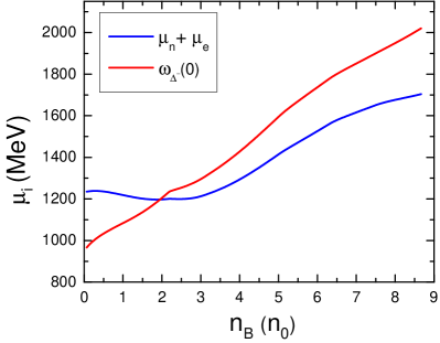
Figure 1: (Color online) Comparison of the neutron-plus-electron effective chemical potential, $\mu_{n}+\mu_{e}$, with the lowest single-particle energy state of the $\Delta^{-}$, $\omega_{\Delta^{-}}(0)$, in NS matter. The presence of $\Delta^{-}$ particles is triggered at the density where the two curves cross, at around $2n_{0}$.

The term $\widetilde{R}=[\partial g_{\rho B}(n)/\partial n]I_{3B}n_{B}\bar{\rho}$ in Eq. (19) is the rearrangement term necessary to guarantee thermodynamic consistency Hofmann et al. (2001). This term also affects the pressure of hadronic matter, which is given by

$$P_{h} = \frac{1}{\pi^{2}}\sum_{B}\int^{p_{F_{B}}}_{0}\!dp\,\frac{p^{4}}{\sqrt{p^{2}+m_{B}^{*2}}}-\frac{1}{2}m_{\sigma}^{2}\bar{\sigma}^{2}$$

$$- \frac{1}{2}m_{\sigma^{*}}^{2}\bar{\sigma^{*}}^{2}+\frac{1}{2}m_{\omega}^{2}\bar{\omega}^{2}+\frac{1}{2}m_{\rho}^{2}\bar{\rho}^{2}+\frac{1}{2}m_{\phi}^{2}\bar{\phi}^{2}$$

$$- \frac{1}{3}\tilde{b}_{\sigma}m_{N}(g_{\sigma N}\bar{\sigma})^{3}-\frac{1}{4}\tilde{c}_{\sigma}(g_{\sigma N}\bar{\sigma})^{4}+n\widetilde{R}.$$

Quantity	SW4L Parameters
$m_{\sigma}$ (GeV)	0.5500
$m_{\omega}$ (GeV)	0.7826
$m_{\rho}$ (GeV)	0.7753
$m_{\sigma^{*}}$ (GeV)	0.9900
$m_{\phi}$ (GeV)	1.0195
$g_{\sigma N}$	9.8100
$g_{\omega N}$	10.3906
$g_{\rho N}$	7.8184
$g_{\sigma^{*}N}$	1.0000
$g_{\phi N}$	1.0000
$\tilde{b}_{\sigma}$	0.0041
$\tilde{c}_{\sigma}$	$-0.0038$
$a_{\rho}$	0.4703

Table 1: Parameters of the SW4L parametrization that lead to the properties of symmetric nuclear matter at saturation density given in Table 2.

Saturation Properties	SW4L
$n_{0}$ (fm-3)	0.150
$E_{0}$ (MeV)	-16.0
$K_{0}$ (MeV)	250.0
$m^{*}_{N}/m_{N}$	0.7
$J_{0}$ (MeV)	30.3
$L_{0}$ (MeV)	46.5

Table 2: Properties of nuclear matter at saturation density, $n_{0}$, obtained for the SW4L parametrization. The entries are: energy per nucleon $E_{0}$, nuclear incompressibility $K_{0}$, effective nucleon mass $m^{*}$, symmetry energy $J_{0}$, and slope of the symmetry energy $L_{0}$.

In this work we use the parameter set SW4L shown in Table 1. The coupling constants as well as the parameters $\tilde{b}_{\sigma}$, $\tilde{c}_{\sigma}$, and $a_{\rho}$ were adjusted according to the properties of nuclear matter at saturation density listed in Table 2.

The scalar meson-hyperon coupling constants $g_{\sigma Y}$ and $g_{\sigma^{*}Y}$ are fit to hyperon ($Y$) single-particle potentials and self-potentials derived from the available empirical data on hypernuclei, once the vector meson-hyperon couplings $g_{\omega Y}$ and $g_{\phi Y}$ have been specified. In SU(3) symmetry the vector couplings are given in terms of the vector mixing angle $\theta_{V}$, the vector coupling ratio $\alpha_{V}$, and the meson singlet-to-octet coupling ratio $z$ Dover and Gal (1984) (see also Schaffner and Mishustin (1996); Spinella (2017); Spinella and Weber (2020, 2019)). The values of these parameters are $\theta_{V}=37.50^{\circ}$, $\alpha_{V}=1$, and $z=0.1949$, corresponding to the SU(3) ESC08 model Rijken et al. (2010).

Once the vector meson-hyperon coupling constants are specified, the scalar meson-hyperon couplings are set to reproduce empirical hyperon single-particle potentials in symmetric nuclear matter at nuclear saturation, $U_{Y}^{~{}\!(N)}(n_{0})$, using the relation Spinella and Weber (2019)

$$U_{Y}^{~{}\!(N)}(n_{0})=g_{\omega Y}\bar{\omega}+g_{\phi Y}\bar{\phi}-g_{\sigma Y}\bar{\sigma}\,.$$ (21)

The following hyperon potentials have been employed: $U_{\Lambda}^{(N)}(n_{0})=-28$ MeV, $U_{\Sigma}^{(N)}(n_{0})=+30$ MeV, and $U_{\Xi}^{(N)}(n_{0})=-14$ MeV. The strange-scalar meson-$\Lambda$ coupling constant $g_{\sigma^{*}\Lambda}$ has been set to reproduce a saturation self-potential of $U_{\Lambda}^{(\Lambda)}(n_{0})=-1$ MeV in isospin-symmetric $\Lambda$-matter, a value close to that suggested by the Nagara event Ahn et al. (2013), using the following,

$$U_{\Lambda}^{~{}\!(\Lambda)}(n_{0})=g_{\omega\Lambda}\bar{\omega}_{0}+g_{\phi\Lambda}\bar{\phi}_{0}-g_{\sigma\Lambda}\bar{\sigma}_{0}-g_{\sigma^{*}\Lambda}\bar{\sigma}^{*}_{0}\,.$$

From this event, the $\Lambda\Lambda$ binding energy was originally determined to be $1.01\pm 0.20$ MeV. This value has subsequently been revised to $0.67\pm 0.17$ MeV Ahn et al. (2013) due to the change of the $\Xi^{-}$ mass by the particle data group. Both values consistently suggest a weak attractive $\Lambda\Lambda$ interaction. We note that values of $U_{\Lambda}^{(\Lambda)}(n_{0})=-1$ or $-5$ MeV have been employed in the literature in the past, while phenomenological relativistic mean-field approaches suggest values between approximately $-14$ and $+9$ MeV, depending on how tight SU(6) constraints are imposed on the approaches Fortin et al. (2017).

The other strange-scalar meson-hyperon couplings are determined relative to that of the $\Lambda$ using $U_{\Xi}^{(\Xi)}(n_{0})=2U_{\Lambda}^{(\Lambda)}(n_{0}/2)$, so that $g_{\sigma^{*}\Sigma}=g_{\sigma^{*}\Lambda}=1.9242$ Oertel et al. (2015). The isovector-vector meson-hyperon coupling constants $g_{\rho Y}$ are given by $g_{\rho\Lambda}=0$ and $g_{\rho\Sigma}=g_{\rho\Xi}=g_{\rho N}$.

To adjust the SW4L parametrization to the nuclear properties of Table 2 we define $x_{\phi B}=g_{\phi B}/g_{\omega N}$. With this definition, the $\phi$–$Y$ coupling ratios are given by $x_{\phi\Lambda}=x_{\phi\Sigma}=1.7855$ and $x_{\phi\Xi}=7.7247$.

Most studies of $\Delta$s in dense matter have been conducted in the standard relativistic mean-field (RMF) approach Waldhauser et al. (1987, 1988); Weber and Weigel (1989b); Choudhury and Rakshit (1993); Cai et al. (2015); Lavagno (2010), the density-dependent RMF approach Drago et al. (2014); Kolomeitsev et al. (2017); Spinella and Weber (2020), or the (density-dependent) relativistic Hartree-Fock approach Weber and Weigel (1989a); Zhu et al. (2016), all indicating at the abundant existence of $\Delta$s in NS matter. We note, however, that a recent study performed for the quark-meson coupling model has suggested that $\Delta$ isobars are absent in NSs Motta et al. (2020). The reason for that are the many-body forces generated by the change in the internal quark structure of the baryons in the scalar mean fields generated in dense nuclear matter.

All of these studies suffer from the problem that the meson–$\Delta$ couplings are only poorly constrained so that particular coupling sets must be chosen with which to conduct the analysis. The meson–$\Delta$ coupling space has been systematically investigated in Ref. Spinella and Weber (2020); Li et al. (2018) and will be further explored and constrained in this work.

To include $\Delta$s in the study of dense NSs matter, we follow a two-pronged approach. First we shall consider a quasi-universal meson–$\Delta$ coupling scheme

$$x_{{\sigma}{\Delta}}=x_{{\omega}{\Delta}}=1.1\,~{}~{}x_{{\rho}{\Delta}}=x_{{\phi}{\Delta}}=1.0\,~{}~{}x_{{\sigma^{*}}{\Delta}}=0.0\,,$$ (22)

where $x_{\sigma^{*}B}\equiv g_{\sigma^{*}B}/g_{\sigma^{*}\Lambda}$ and $g_{\sigma^{*}\Lambda}=1.9242$. Next, we explore the parameter space of the $\sigma$–$\Delta$ coupling constant, related with the effective $\Delta$ mass, $m_{\Delta}^{*}$, considering the constraint imposed by the event GW170817 on NSs radii. We study coupling ratios in the interval $1.1\leq x_{\sigma\Delta}\leq 1.258$. The lower bound $x_{\sigma\Delta}=1.1$ (together with $x_{\omega\Delta}=1.1$, $x_{\rho\Delta}=1.0$) satisfied the constraints on the potential of $\Delta$s in symmetric nuclear matter at saturation density Spinella and Weber (2020); Drago et al. (2014); Kolomeitsev et al. (2017); Riek et al. (2009). The upper bound $x_{\sigma\Delta}=1.258$ is determined by the microscopic stability of matter, that is, for values $x_{\sigma\Delta}>1.258$ pressure is no longer monotonously increasing with density so that the matter becomes microscopically unstable.

IV The Quark Phase

For the description of quark matter, including diquarks in the SU(3) non-local model, we use the Lagrangian given by

$$\mathcal{L} = \bar{\psi}(x)(-i\not{\partial}+\hat{m})\psi(x)-\frac{G_{s}}{2}\big{[}j_{a}^{s}(x)j_{a}^{s}(x)+$$ (23)

$$+ j_{a}^{p}(x)j_{a}^{p}(x)\big{]}+\frac{G_{v}}{2}j_{a}^{\mu}(x)j_{a}^{\mu}(x)$$

$$- \frac{H}{4}A_{abc}\big{[}j_{a}^{s}(x)j_{b}^{s}(x)j_{c}^{s}(x)-3j_{a}^{s}(x)j_{b}^{p}(x)j_{c}^{p}(x)\big{]}\,,$$

where $A_{abc}$ are constants given in terms of the Gell-Mann matrices and $j_{a}^{s}(x)$, $j_{a}^{p}(x)$ and $j_{a}^{\mu}(x)$ are interaction currents. The current quarks masses and the coupling constants $G_{s}$, $H$, and $\Lambda$ are taken from Ref. Malfatti et al. (2019). The vector interaction coupling constant, $G_{v}$, is expressed in terms of the scalar coupling constant, $G_{s}$, and is treated as a free parameter.

To include diquark channels in the model, an additional term of the form

$$\mathcal{L}_{D}=-\frac{G_{D}}{2}\left[j_{D}\left(x\right)\right]^{\dagger}j_{D}\left(x\right)\,,$$ (24)

needs to be added to Eq. (23). Here $G_{D}$ is the diquark coupling constant expressed in multiples of $G_{s}$. The diquarks currents are given by

$$j_{D}\left(x\right)=\int d^{4}\,zg(z)\overline{\psi}_{C}\left(x+\frac{z}{2}\right)i\gamma^{5}\lambda_{A}\lambda_{A^{\prime}}\psi\left(x-\frac{z}{2}\right)\,,$$ (25)

where $\psi_{C}=\gamma_{2}\gamma_{4}\overline{\psi}^{T}(x)$. The matrices $\lambda_{A}$ and $\lambda_{A^{\prime}}$ operate in the color and flavor spaces, respectively, and take on values ${2,5,7}$ (see Appendix A for details). The non-local regulator $g(x-y)$ is related to its momentum space representation, $g(p)$, via

$$g(x-y)=\int\frac{d^{4}p}{(2\,\pi)^{4}}\,e^{i(x-y)p}\,g(p)\,.$$ (26)

The inclusion of color superconductivity leads to a matrix for the diquark condensates that can be written as

$$s_{AA^{\prime}}=\langle\overline{\psi}_{C}\gamma_{5}\lambda_{A}\lambda_{A^{\prime}}\psi\rangle\,,$$ (27)

where $C=\gamma_{2}\gamma_{4}$ is the operator of charge conjugation. This matrix can be simplified by a color rotation,

$$s=\begin{pmatrix}s_{22}&0&0\\ s_{52}&s_{55}&0\\ s_{72}&s_{75}&s_{77}\\ \end{pmatrix}\,.$$ (28)

The non-diagonal matrix components are negligible in the one-gluon exchange regime Alford et al. (1999); Fritzsch et al. (1973), so that one only needs to keep the elements $s_{22}$ , $s_{55}$, and $s_{77}$. In this work, we consider the formation of $(u_{r},d_{g})$ and $(u_{g},d_{r})$ diquark pairs. Therefore

$$s_{22}=\langle\overline{\psi}\gamma_{5}\lambda_{2}\lambda_{2}^{\prime}\psi\rangle\,,\quad s_{55}=s_{77}=0\,.$$ (29)

Including the new diquark bosonic field $\bar{\Delta}$ and its associated auxiliary field $\bar{D}$, we bosonize the euclidean effective action, $S_{E}$, which follows from Eq. (23). Then, in the mean-field approximation,

$$\frac{S_{E}^{MFA}}{V^{(4)}} = -2\,\mathrm{Tr}\,\int\,\frac{d^{4}p}{(2\,\pi)^{4}}\,\mathrm{ln}\,A(p)\,-$$ (30)

$$- \frac{1}{2}\left[\left(\bar{\sigma}_{a}\bar{S}_{a}+\frac{G_{s}}{2}\bar{S}_{a}\,\bar{S}_{a}+\bar{\theta}_{a}\bar{V}_{a}-\frac{G_{v}}{2}\bar{V}_{a}\,\bar{V}_{a}\right)\right.$$

$$+ \left.\frac{H}{2}A_{abc}\bar{S}_{a}\bar{S}_{b}\bar{S}_{c}+2\bar{\Delta}\bar{D}+G_{D}\bar{D}\,\bar{D}\right]\,,$$

where $A(p)$ is the inverse of the quark propagator with interactions and $\bar{S}_{a}$ and $\bar{V}_{a}$ are the mean-field values of the auxiliary fields corresponding to $\bar{\sigma}_{a}$ and $\bar{\theta}_{a}$, respectively. After some algebra in the first term of Eq. (30) (see Appendix A for details) the regularized thermodynamic potential for the 2SC+s phase reads

$$\Omega= - 2\sum_{c}\int\frac{d^{4}p}{(2\pi)^{4}}\left\{\mathrm{ln}\left[\frac{{q_{sc}^{+}}^{2}+M_{sc}^{2}}{p_{sc}^{2}+m_{s}^{2}}\right]-\frac{1}{2}\mathrm{ln}|A_{c}|^{2}\right.$$ (31)

$$- \left.\mathrm{ln}[({p_{uc}^{+}}^{2}+m_{u}^{2})({p_{dc}^{+}}^{2}+m_{d}^{2})]\right\}$$

$$- \frac{1}{2}\sum_{f}\left[\left(\bar{\sigma}_{f}\bar{S}_{f}+\frac{G_{S}}{2}\bar{S}_{f}^{2}+\bar{\theta}_{f}\bar{V}_{f}-\frac{G_{V}}{2}\bar{V}_{f}^{2}\right)\right.$$

$$+ \left.\frac{H}{2}\bar{S}_{u}\bar{S}_{d}\bar{S}_{s}+2\bar{\Delta}\bar{D}+G_{D}\bar{D}^{2}\right]-\Omega_{free}^{Reg}\,.$$

All the quantities in Eq. (31) including the expression for $\Omega_{free}^{Reg}$ are given in Sect. A. From the following set of (seven) coupled equations,

$$\frac{\partial\Omega}{\partial\bar{\sigma}_{f}}=0\,,\quad\frac{\partial\Omega}{\partial\bar{\theta}_{f}}=0\,,\quad\frac{\partial\Omega}{\partial\bar{\Delta}}=0\,,$$ (32)

it is possible to determine the mean-field values of $\bar{\sigma}_{f}$, $\bar{\theta}_{f}$, and $\bar{\Delta}$.

V Results and Discussion

In Fig. 2 we compare the EoSs of this work with bounds on the EoS recently established in Ref. Annala et al. (2020). The bands cover a large number of EoSs generated with the speed-of-sound interpolation method.

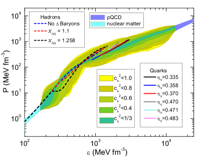
Figure 2: (Color online) Comparison of the EoSs of this work with bounds on the EoS recently established in Ref. Annala et al. (2020).

As can be seen, all our models lie comfortably within the bounds on the neutron star matter EoS shown in Fig. 2.

In Fig. 3, we show the mass-radius relationships of stellar configurations, computed for the hadronic SW4L EoS of this work, for different values of the $\sigma$–$\Delta$ coupling ratio $x_{\sigma\Delta}$. All the three mass-radius relationships obey the gravitational-mass constraint set by $2\,M_{\odot}$ pulsars as well as the radius constraints extracted from NICER observations Riley et al. (2019); Miller et al. (2019) and the gravitational-wave event GW170817 Capano et al. (2020).

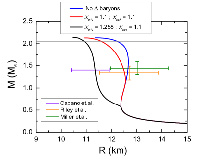
Figure 3: (Color online) Mass-radius relationships of compact stars computed for purely hadronic matter, based on the SW4L parametrization introduced in Sect. III. The observed radius constraints are taken from Refs. Riley et al. (2019); Miller et al. (2019) (orange and green horizontal lines, respectively) and Ref. Capano et al. (2020) (purple horizontal line). The gray horizontal line shows the minimum gravitational mass established for PSR J0740+6620 Cromartie et al. (2020).

As can be seen in Fig. 3, the impact of $\Delta$ baryons on the mass-radius relationship is strong for $\sigma$–$\Delta$ coupling ratios in the range of $1.1\leq x_{\sigma\Delta}\leq 1.258$. The mass-radius relationships of this figure are computed for a $\omega$–$\Delta$ coupling constant ratio of $x_{\omega\Delta}=1.1$. We found that if we set $x_{\sigma\Delta}$ = $x_{\omega\Delta}$, the minimum coupling value for the EoS to remain microscopically stable ($c_{s}>0$) is $x_{\sigma\Delta}$ = 1.1. Varying $x_{\sigma\Delta}$ while keeping $x_{\omega\Delta}$ at 1.1 changes the maximum NS mass insignificantly, but the radii of all stars decrease if $x_{\sigma\Delta}>x_{\omega\Delta}$ and increase significantly if $x_{\sigma\Delta}<x_{\omega\Delta}$, where $x_{\sigma\Delta}=1.258$ sets the upper limit for which $c_{s}>0$ holds for $x_{\omega\Delta}=1.1$. Finally, the mass-radius relationships are virtually the same if $x_{\sigma\Delta}=x_{\omega\Delta}$ regardless whether $x_{\sigma\Delta}=1.1$ or 1.258. As can be seen in Fig. 3, current observational constrains on the radius of a $\sim 1.5\,M_{\odot}$ NS are reproduced by our models for $1.1\leq x_{\sigma\Delta}\leq 1.258$. The hope is that future observational constraints will allow one to narrow down this range and to draw firm conclusions on the possible existence of $\Delta$s in NSs.

In summary, we note that the presence of $\Delta$s in NS matter strongly modifies the radii of NSs. The $2\,M_{\odot}$ mass constraint can nevertheless be fulfilled comfortably. This is in agreement with what has been found in other studies Schürhoff et al. (2010); Li et al. (2018); Kolomeitsev et al. (2017); Ribes et al. (2019).

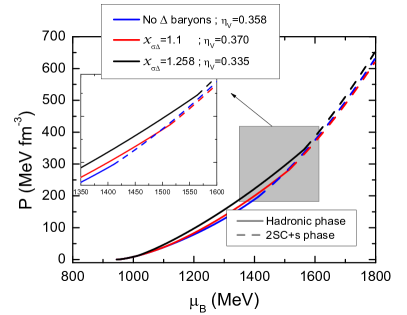
Figure 4: (Color online) Illustration of the hybrid EoSs computed in this work. Quark matter is treated as a 2SC+s color superconductor. The inset figure shows the pressures of the different phases of matter in the phase transition region.

The radii of NSs with canonical masses between 1.4 to $1.5\,M_{\odot}$ turn out to be particularly sensitive to the presence of $\Delta$s. They may change by up to $\sim 1.5$ km for the theoretically defensible sets of meson–hyperon (SU(3) ESC08 model) and meson–$\Delta$ coupling constants of this work.

In Fig. 4, we show the results for the hybrid EoS computed for the models introduced in Sects. III and IV. The solid lines mark the region where matter exists solely in the hadronic matter phase and the dashed lines mark the region where the matter exists in the form of quark matter in the 2SC+s color superconducting phase. Also shown in this figure is the impact of $\Delta$ baryons on the EoS, which depends on the $x_{\sigma\Delta}$ coupling ratio as discussed just above, and the role of the quark vector interaction value, $\eta_{v}$ ($\equiv G_{v}/G_{s}$), whose value determines the pressure at which the hadron-quark phase transition takes place. The 2SC+s phase is always energetically favored relative to normal (i.e., non-superconducting) quark matter, as shown in Fig. 5. Moreover, this result is independent of the vector interaction value considered. We therefore

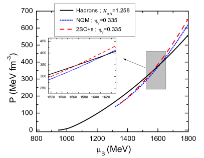
Figure 5: (Color online) Comparison of hybrid EoSs. NQM refers to ordinary non-superconducting quark matter, 2SC refers to quark matter in the 2SC+s superconducting phase. The latter turns out to be energetically favored at high chemical potentials. The inset figure shows the pressures in the phase transition region.

find that a direct transition from hadronic matter to 2SC+s color superconducting quark matter for our model, bypassing ordinary quark matter. The inset figure shows the pressures of the different phase of matter in the phase transition zone. We can see that when the $x_{\sigma\Delta}$ coupling constant ratio is increased, the transition pressure increases as well. Moreover, larger values of the vector interaction lead to a stiffer EoS.

In Fig. 6, we show the particle populations of neutron star matter computed for the hadronic EoSs of this work. In the top panel we show how the composition looks like if the $\Delta$ baryon is not taken into account in the calculation. The other two panels show the hadronic populations if all states of the $\Delta$ baryon ($\Delta^{++}$, $\Delta^{+}$, $\Delta^{0}$, $\Delta^{-}$) are taken into account in the calculation. Naively, one would assume $\Delta$s would not be favored in NS matter for several reasons Spinella and Weber (2020). First, their rest mass is greater than the rest masses of both the $\Lambda$ and $\Sigma$ hyperons. Second, negatively charged baryons are generally favored as their presence reduces the high Fermi momenta of the leptons, but the $\Delta^{-}$ has triple the negative isospin of the neutron ($I_{3\Delta^{-}}=-3/2$), and thus its presence should be accompanied by a substantial increase in the isospin asymmetry of the system. These arguments, however appear to be largely invalid for the following reasons. Incorporating the repulsive saturation potential of the $\Sigma$ hyperon into the determination of the meson–$\Sigma$ coupling constants greatly reduces the $\Sigma$’s favorability (it is totally absent in the compositions shown in Fig. 6), and thus it is not likely to compete with the $\Delta^{-}$ state. More importantly the overall effect of the asymmetry energy on the system is significantly reduced when one employs a parametrization with a density-dependent isovector meson–baryon coupling constant as done in this work (SW4L), which is necessary to satisfy the constraints on the slope of the asymmetry energy at saturation density Spinella and Weber (2020).

The values of the $\sigma$–$\Delta$ coupling ratio are $x_{\sigma\Delta}=1.1$ and $x_{\sigma\Delta}=1.258$. As a reminder, the latter value constitutes the maximum possible value allowed by microscopic stability of the matter. We see that the appearance of the charged states of the $\Delta$ baryon is sequential, beginning with the $\Delta^{-}$ at less than twice nuclear saturation density and ending with the $\Delta^{++}$ at densities as low as around 4 times nuclear saturation density, depending on the value of $x_{\sigma\Delta}$.

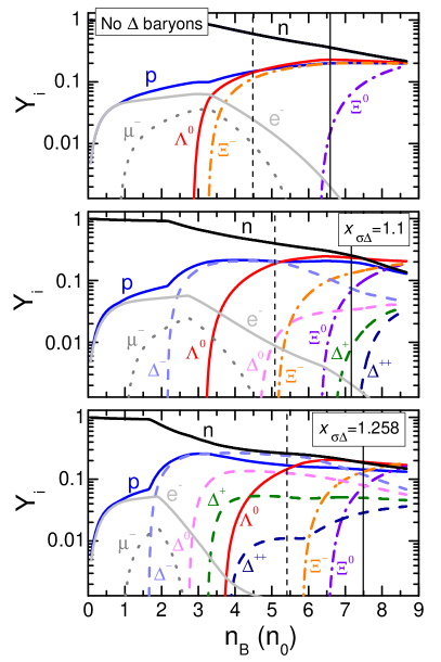
Figure 6: (Color online) Baryon-lepton populations of the neutron stars shown in Fig. 3. The solid vertical lines mark the central densities of the maximum-mass stars associated with these compositions. The dashed vertical lines mark the densities at which phase equilibrium with 2SC+s quark matter would set in.

Based on these populations, $\Delta$ baryons are abundantly present in NS matter already at densities that are markedly smaller than the densities of the maximum-mass neutron stars (solid vertical lines) associated with these compositions. Even NSs with a masses in the range between 1.4 to $1.5\,M_{\odot}$ would possess significant populations of $\Delta$s, which, as was shown in Fig. 3, significantly modifies the radii of these objects. We also note that the $\Delta$ population sets in at densities that are less than the density at which the hadron-quark phase transition would set in (vertical dashed lines in Fig. 6) for this parametrization. This is most evident for the maximum possible value of the $\sigma$–$\Delta$ coupling ratio, $x_{\sigma\Delta}=1.258$, in which case all charged $\Delta$ states are present well before the threshold density at which quark deconfinement sets in. It is interesting to note that, at over certain density ranges, the $\Delta^{-}$ abundances are comparable to those of protons and $\Lambda$s. Given the impact $\Delta$s may have on the masses and radii of NSs, one might hope that future astrophysical observations of these and other NS quantities (e.g., moment of inertia) will help to elucidate the relevance of $\Delta$s for dense nuclear matter studies.

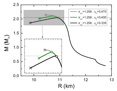
Figure 7: Mass-radius relationships obtained with the hybrid EoS for different vector repulsion parametrizations. The hollow circles indicate the onset of quark matter and the crosses mark the terminal mass model of each stellar sequence.

V.1 Extended branch of stable hybrid stars

The confinement/deconfinement process is not solely ruled by the strong interaction, whose timescale is $\sim 10^{-23}$ s. Other physical phenomena like Coulomb screening and surface and curvature effects play important roles (see Ref. Lugones and Grunfeld (2017), and references therein). Moreover, it is important to stress that the strong interaction operates on time-scales that are shorter (by several orders of magnitude) than those related to the weak interactions. For this reason, the weak interaction cannot operate during the deconfinement process. In view of that, newly deconfined quark matter is transitorily out of chemical equilibrium and the abundances per baryon of each particle need to be the same in both phases. Several model-dependent calculations show that if quark matter is to be produced preserving flavor, its final equilibrium state is not accessible directly and a two-step transition between hadronic and quark matter must take place, firstly to a flavor preserving out of $\beta$-equilibrium quark state, followed by a second weak decay to the final equilibrium quark state in $\sim 10^{-8}$ s (see, for example, Ref. Lugones (2016), and references therein).

Since there is no high-density EoS constructed from first-principles, it is not clear whether a fluid element that oscillates around the transition pressure will suffer a slow or rapid direct conversion. Several works have shown that the probability of a hadron-quark phase transition is related to a model-dependent timescale (see, for example, Refs. Lugones and Grunfeld (2011); Bombaci et al. (2016); Lugones (2016), and references therein). In addition, there are some results that indicate this timescale is around $\sim 10^{-3}$ s Haensel et al. (1989) or even larger (see, for example, Refs. Iida and Sato (1998); Bombaci et al. (2004, 2009)). These theoretical studies indicate that the hadron-quark phase transition should be considered to be slow. Because of these theoretical uncertainties, we consider both the slow and rapid conversion scenarios between hadronic and quark matter and analyze their astrophysical implications.

In Fig. 7, we show the mass-radius relationship of HSs for a fixed value of $x_{\sigma\Delta}$ but different values of the vector repulsion parameter $\eta_{v}$. The onset of quark matter in the cores of these stars is marked with hollow circles. It can be seen that quark deconfinement occurs only for stars very close to the maximum-mass peak of each stellar sequence. This is in agreement with results reported in the literature previously (see, for example,

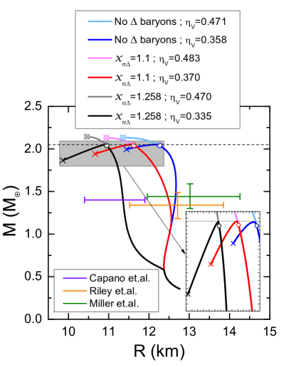
Figure 8: (Color online) Mass-radius relationships obtained with the hybrid EoS of this work ($x_{\omega\Delta}=1.1$). The constraints on $M$ and $R$ are the same as in Fig. 3. The hollow circles mark the onset of quark deconfinement. The extended branches of stable HSs terminate at the crossed locations.

Refs. Ranea-Sandoval, Ignacio F. and Han, Sophia and Orsaria, Milva G. and Contrera, Gustavo A. and Weber, Fridolin and Alford, Mark G. (2016); Malfatti et al. (2019); Mariani et al. (2019), and references therein), where it was shown that the rapid conversion of hadronic matter to quark matter in HSs tends to destabilize such objects. For a rapid conversion, the timescale associated with transforming hadronic matter to quark matter in a star is much shorter than the timescale set by the stellar perturbations oscillations Pereira et al. (2018); Mariani et al. (2019). The situation is dramatically different if the conversion proceeds slowly, that is, if the timescale associated with transforming hadronic matter to quark matter is much larger than the timescale set by the stellar perturbations. In the latter case, a new (extended) branch of stable HSs can exist, ranging from the maximum-mass star of a sequence to a new terminal-mass configuration Pereira et al. (2018); Mariani et al. (2019). They are marked with crosses in Fig. 7. As shown in Refs. Pereira et al. (2018); Mariani et al. (2019) the usual static stability condition against gravitational collapse, $\partial M/\partial\epsilon_{c}\geq 0$ (where $\epsilon_{c}$ is the central energy density of a star) always holds for a rapid hadron-to-quark conversion, but does not determine stability against gravitational collapse if the conversion is slow.

The stellar configurations in the extended stability branch are stable against all radial perturbations (considering linear perturbations). For this reason, their lifetimes are the same as those of the ”traditional” stable branch. In all the models we have considered, the central density of the terminal-mass configuration object is less than 3000 MeV/fm³ (see, Fig. 12 for more details).

As can be seem from Fig. 7, the radii of HSs in the extended stellar branch may differ from the radii of stars made entirely of hadronic matter by up to $\sim 1$ km. This property, therefore, could serve as a distinguishing features between both types of stars.

Another observation to be made from Fig. 7 concerns the role of the strength of the vector interaction among quarks, $\eta_{v}$. As can be seen, increasing the value of $\eta_{v}$ leads greater maximum stellar masses, while, at the same time, the extended branches of the HSs shrink. The upper limit on the value of $\eta_{v}$ is obtained when the extended branch has shrunk to zero, in which case stability ends at the maximum-mass star of the stellar sequence. In what follows, we will study two limiting cases for $\eta_{v}$, one where its value is determined by the conventional maximum-mass stability criteria mentioned just above (denoted $\eta_{v,{\rm max}}$). The other case corresponds to the minimum value of $\eta_{v}$ (denoted $\eta_{v,{\rm min}}$) determined by the requirement that at least $2.05\,M_{\odot}$ be obtained with our models. These cases are shown in Fig. 8 for stellar populations with and without $\Delta(1232)$ isobars. If no $\Delta$s are taken into account, the minimum and maximum values for $\eta_{v}$ are $\eta_{v,{\rm min}}=0.358$ and $\eta_{v,{\rm max}}=0.471$. If $\Delta$s are taken into account in the calculation, we have $\eta_{v,{\rm min}}=0.370$ and $\eta_{v,{\rm max}}=0.483$ for a relative $\sigma$–$\Delta$ coupling of $x_{\sigma\Delta}=1.1$, and $\eta_{v,{\rm min}}=0.335$ and $\eta_{v,{\rm max}}=0.470$ for $x_{\sigma\Delta}=1.258$.

In Fig. 9 we show the square of the speed of sound, $c_{s}^{2}$, as a function of baryon number density for the hybrid star EoS with color superconductivity. The locations of the maximum-mass stars are marked with vertical bars and the crosses show the stellar models at the endpoints of stability. The erratic behavior of $c_{s}^{2}$ below around $4\,n_{0}$ has its origin in the $\Delta$ population (see Fig. 6), which depends on the $\sigma$–$\Delta$ coupling ratio $x_{\sigma\Delta}$. A case in point is $x_{\sigma\Delta}=1.258$, for which the $\Delta^{-}$ population sets in at densities even less than $2\,n_{0}$, leading to a sharp drop in $c_{s}^{2}$.

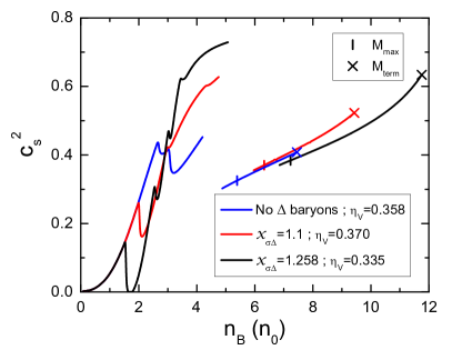
Figure 9: (Color online) Square of the speed of sound, $c_{s}^{2}$, as a function of normalized baryonic number density, $n_{B}/n_{0}$, for different values of the vector repulsion parameter $\eta_{v}$.

The zig-zag behavior of $c_{s}^{2}$, therefore, is the more prominent the larger the value of $x_{\sigma\Delta}$. The speed of sound in the quark phase, which is present at densities greater than $\sim 5\,n_{0}$, violates the so-called conformal limit of $c_{s}^{2}\leq 1/3$ (a discussion if this limit can be found it Refs. Bedaque and Steiner (2015); Tews et al. (2018)) and reaches values of up to 0.8 in the cores of HSs at the terminal mass ($M_{\rm term}$). The actual value of $c_{s}$ depends, like it is the case for hadronic matter, on the stiffness of the hybrid EoS which, in turn, is determined by the value of the strength of the vector interaction, $\eta_{v}$. We note that in order to obtain heavy ($\sim 2\,M_{\odot}$) NSs combined with relatively small radii in the 10 to 12 km range (Fig. 3), a rapid increase in pressure in the core of a NS is required. This implies a non-monotonic behavior of the speed of sound in dense NS matter, which is obtained naturally if the matter in the cores of NSs is no longer described in terms of nucleons only Tews et al. (2018).

V.2 Notes on the mixed hadron-quark phase

Even for the smaller values of $\eta_{v}$ studied in this paper, we obtain hybrid stars with only a modest amounts of matter in the mixed hadron-quark phase. This feature can be inferred graphically from Fig. 10, where we show the pressure in the quark-hadron transition region obtained for the Gibbs and the Maxwell treatment. For the Gibbs phase transition (dashed line) we find that the mixed phase exists only for baryon chemical potentials in the small range of $1563~{}{\rm MeV}\lesssim\mu_{B}\lesssim 1568~{}{\rm MeV}$. It can also be seen that the phase transition occurs not until relatively high pressure values are reached.

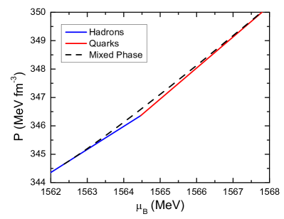
Figure 10: (Color online) Pressure as a function of baryon chemical potential, for the Maxwell (solid lines) and Gibbs (dashed line) construction.

We note that we have assumed a surface tension between the confined and deconfined phases of $\sigma_{HQ}=0$ when constructing the mixed phase and have not taken into account the possibility of structure formation in the mixed phase Glendenning (2001); M. Spinella et al. (2016); Weber et al. (2019). A comparison of our results for the EoS shown in Fig. 11 with those of Ref. Maslov et al. (2019) leads us to conclude that the formation of a Gibbs mixed phase is not favored by our models and that the phase transition ought to be Maxwell-like. Moreover, it can be seen from Fig. 10 that we obtain a narrow mixed phase region for the Gibbs construction of the phase transition. The situation is the same for all the hybrid EoS parameters: the result is a short mixed phase region of constant pressure inside the star with a sharp interface boundary between hadronic and quark matter. If $\sigma_{QH}\neq 0$, this would suggest that the formation of geometrical structures due to charge rearrangement in the mixed phase is energetically disfavored, and that the Gibbs phase transition becomes a Maxwell phase transition Maslov et al. (2019).

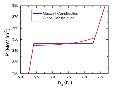
Figure 11: (Color online) Pressure as a function of baryon number density, in units of the nuclear saturation. The phase transition is modeled as both a Maxwell and a Gibbs transition.

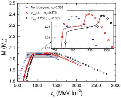
Figure 12: (Color online) Gravitational mass as a function of central energy density for the hybrid EoS of this work. The enlarged region shows the results obtained for the Maxwell (dotted lines) or Gibbs (continuous line) constructions.

The mass-radius relationships obtained for the Gibbs and the Maxwell treatments are however very similar to each other, except that the Gibbs stellar sequence terminates at the maximum-mass configuration of this sequence, while the Maxwell sequence extends stably beyond the maximum-mass configuration, ending at the terminal mass (see Sect. V.1). This can be seen also in Fig. 12. From the enlarged region in this plot, one sees that no mixed phase formation is possible if $\Delta$ baryons are absent (stellar configurations marked with blue horizontal bars). Both Maxwell and Gibbs constructions are possible for the two limiting values of $x_{\sigma\Delta}=1.1$ (red crosses and continuous red line) and $x_{\sigma\Delta}=1.258$ (black hollow circles and black line).

V.3 Tidal deformability

A new observational window on the inner workings of NSs is provided by the gravitational-wave peak frequency and the stellar tidal deformability of NSs in binary NS mergers Bauswein et al. (2019). The binary tidal deformability is given by

$$\tilde{\Lambda}=\frac{16}{13}\frac{(12q+1)\Lambda_{1}+(12+q)q^{4}\Lambda_{2}}{(1+q)^{5}}\,,$$ (33)

where $q=M_{2}/M_{1}$ is the ratio of the masses of the merging neutron stars and $\Lambda_{1,2}$ their dimensionless tidal deformabilities, which can be calculated by solving an additional differential equation together with the Tolman-Oppenheimer-Volkoff stellar structure equations Hinderer (2008); Han and Steiner (2019).

The tidal deformabilities of the two binary components of GW170817 has been estimated by the LIGO-VIRGO collaboration Abbott et al. (2017). Although some concerns regarding an apparent discrepancy between data coming from Handford and Livingstong LIGO detectors has been recently raised Narikawa et al. (2019), there is agreement on the validity and strength of the general results obtained by both collaborations. The tidal deformability has been used to eliminate several EoS that have been used in the past to describe the matter in the cores of NSs (see Ref. Orsaria et al. (2019), and references therein).

In Fig. 13 we present the tidal deformabilities $\Lambda_{1}$ and $\Lambda_{2}$ computed for the NSs shown in Fig. 3. The black (gray) curve in this figure denotes the 50% (90%) confidence level curve obtained in Ref. Abbott et al. (2017) for the low-spin scenario. One sees that

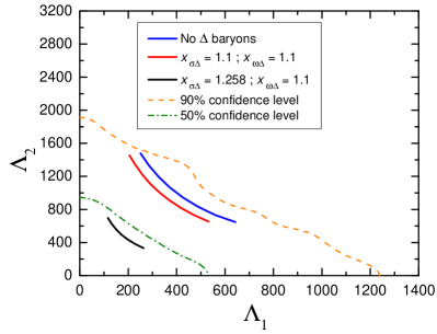
Figure 13: (Color online) Dimensionless tidal deformabilities $\Lambda_{1}$ and $\Lambda_{2}$ for the hadronic configurations of Fig. 3. The orange (cyan) dashed lines represents the 50% (90%) confidence limit of the probability contour of GW170817.

the presence of $\Delta$s leads to a better agreement with the observed data of GW170817. It is not possible to extract any information related to the appearance of quark matter from the tidal deformability data of GW170817 as the masses of the objects in this BNS are lower than the masses at which our models predict the existence of quark matter in NSs. Event GW190425 involved more massive NSs Abbott et al. (2020). But this event was only observed by the LIGO Livingston detector and no electromagnetic counterpart was detected either so that the data from this merger are less constraining and informative than those of GW170817.

VI Conclusions

In this work we have presented a hybrid EoS which leads to masses which satisfy the latest constraints established by massive pulsars and a hadronic EoS satisfying the restrictions on radii set by gravitational-wave data and NICER data. To describe matter in the stellar cores of NSs, we have included (in addition to hyperons) all charged states of the $\Delta(1232)$ baryon in a non-linear density dependent mean-field treatment based on the SW4L parametrization and studied the impact of these particles on the masses and radii of NSs. Specifically the latter depend rather sensitively on the value of the $\sigma$–$\Delta$ coupling ratio, $x_{\sigma\Delta}=g_{\sigma\Delta}/g_{\sigma N}$, which has been taken to be between 1.1 and its maximum-possible value of 1.258 set by the microscopic stability of the matter. We found that varying $x_{\sigma\Delta}$ in this range changes the radii of NSs by up to $\sim 1.5$ km, depending on gravitational mass. The speed of sound, $c_{s}$, of hadronic matter remains always less than the speed of light for $1.1\leq x_{\sigma\Delta}\leq 1.258$, so that the hadronic EoSs are causal at all densities. Depending on the value of $x_{\sigma\Delta}$, we find that the presence of $\Delta$s in NS matter drastically alters the speed of sound, which then would no longer be a monotonically increasing with density, which allows one to accommodate heavy NSs with relatively small radii in the 10 to 12 km range.

Quark matter is modeled in the framework of the SU(3) non-local NJL model. The effects of color superconductivity on the EoS has been taken into account by considering the 2SC+s diquark condensation pattern, for the first time, in a non-local NJL model. Compared to normal quark matter, the 2SC+s phase is generally energetically favored over normal quark matter at all densities. A sequential phase transition from hadronic matter, to normal quark matter, to 2SC+s quark matter would only be possible if the hadron-quark phase transition were to occur at the same density at which normal quark matter turns into 2SC+s matter. Compared to the non-color superconducting case, the inclusion of 2SC+s color superconductivity softens the EoS mildly, which in turn decrease of the maximum HS mass. Nevertheless, it is still possible to satisfy the $2\,M_{\odot}$ constraint set by the most massive NSs observed to date.

We have constructed the phase transition to quark matter using both the Maxwell and Gibbs descriptions. If the phase transition is treated as being sharp (Maxwell), so that no mixed phase exists, two possible scenarios emerge: either a rapid or a slow phase transition. As was found in several previous works Ranea-Sandoval, Ignacio F. and Han, Sophia and Orsaria, Milva G. and Contrera, Gustavo A. and Weber, Fridolin and Alford, Mark G. (2016); Malfatti et al. (2019), assuming a slow phase transition extends the region of stable stars beyond the maximum-mass star of a given stellar sequence, leading to new stellar configurations that are more compact than the stars along the traditional branch. The stars on the extended branch have the same mass as their counterparts on the traditional branch, but their respective radii differs by up to 1 km leading to twin-like stellar configurations. When a rapid phase transition is assumed to occur, on the other hand, the extended branch vanishes and one is left with only the traditional branch of stable configurations. In this case, the appearance of a quark matter in the cores of NSs almost immediately destabilizes them (aside from a very short portion on the traditional branch), in agreement with the results of previous works (see, for example, Refs. Ranea-Sandoval, Ignacio F. and Han, Sophia and Orsaria, Milva G. and Contrera, Gustavo A. and Weber, Fridolin and Alford, Mark G. (2016); Malfatti et al. (2019), and references therein).

As shown recently in Ref. Pereira et al. (2018), treating the hadron-quark phase transition as a sharp Maxwell transition leads to stable compact stars that, remarkably, lie beyond the maximum-mass peak of a stellar sequence (the extended branch). This extended branch exists only for the Maxwell transition, but disappears if the phase transition is treated as a smooth Gibbs transition. The stars on the extended branch contain pure quark matter in their cores, in sharp contrast to the stars on the conventional branch which, at best, contain only small amounts of quark matter mixed with hadronic matter. The surface tension is known to play a critical role when modelling the hadron-quark phase transition in terms of either a Maxwell or Gibbs transition. If either one of them has its physical correspondence in the core of a compact star, the discussion of this paragraph may help to shed light on the unknown value of the surface tension $\sigma_{HQ}$ between the confined and deconfined phases Glendenning (2001); M. Spinella et al. (2016); Weber et al. (2019); Maslov et al. (2019).

Possible observable features that may allow one to distinguish between stars on the conventional branch and stars on the extended branch are differences in the stellar radii, which could be as large as around 1 km, and the non-radial quasi-normal modes, such as g-modes. As shown, for instance, in Refs. Miniutti et al. (2003); Sotani et al. (2011); Vásquez Flores and Lugones (2014); Ranea-Sandoval et al. (2018); Orsaria et al. (2019), g-modes are only present in compact stars if the nuclear EoS contains a sharp (i.e., constant pressure) density discontinuity.

We also calculated the individual tidal deformabilities $\Lambda_{1}$ and $\Lambda_{2}$ of merging NSs for our hadronic EoSs. The results are consistent with the observational constraints from the analysis of GW170817 data. This is very interesting as it shows that a hadronic EoS which includes all particles of the baryonic octet plus all charged states of the $\Delta(1232)$ is in agreement with present gravitational-wave data, as well as the latest observed data on masses and radii of NSs.

Appendix A Details on the treatment of the 2SC+s phase

Working in SU(3), we can write the operator $A(p)$ of Eq. (30) in a compact form,

$$A(p)=\begin{pmatrix}-\not{p}+\hat{M}+i\hat{\mu}\gamma^{4}&i\sum_{A}\Delta_{A}^{p}\gamma_{5}\lambda_{A}\lambda_{A}\\ i\sum_{A}(\Delta_{A}^{p})^{*}\gamma_{5}\lambda_{A}\lambda_{A}&-\not{p}+\hat{M}-i\hat{\mu}\gamma^{4}\\ \end{pmatrix}\,,$$ (34)

where $\Delta_{A}^{p}=\Delta_{A}g(p)$. This operator is a 72 $\times$ 72 matrix in Dirac, flavor, color and Nambu-Gorkov spaces. However, it is possible to evaluate the trace in Eq. (30). Note the matrix of Eq. (34) is the inverse fermion propagator, where $\hat{M}=\mathrm{diag}(M_{u},M_{d},M_{s})$ Buballa (2005). Then, rearranging rows and columns, and using the logarithm trace notation we can write

$$\mathrm{Tr}\{\mathrm{ln}[A(p)]\}= \mathrm{Tr}[\mathrm{ln}(M_{ug,dr})]+\mathrm{Tr}[\mathrm{ln}(M_{ur,dg})]$$ (35)

$$+ \mathrm{Tr}[\mathrm{ln}(M_{ub,sr})]+\mathrm{Tr}[\mathrm{ln}(M_{ur,sb})]$$

$$+ \mathrm{Tr}[\mathrm{ln}(M_{db,sg})]+\mathrm{Tr}[\mathrm{ln}(M_{dg,sb})]$$

$$+ \mathrm{Tr}[\mathrm{ln}(M_{ur,dg,sb})]\,.$$

In the framework of the 2SC+s phase, $\Delta_{2}\neq 0$ and $\Delta_{5}=\Delta_{7}=0$. Thus, the matrices $M_{f,f^{\prime}}$ of Eq. (35) involving the quark strange do not have diagonal components and such quark decouples. Finally, the only matrix structure involving diquarks in a compact form is given by

$$M_{ud}=\begin{pmatrix}-\not{p}+\hat{M}+i\hat{\mu}\gamma^{4}&i\Delta_{2}^{p}\gamma^{5}\\ i\Delta_{2}^{p}\gamma^{5}&-\not{p}+\hat{M}-i\hat{\mu}\gamma^{4}\\ \end{pmatrix}\,,$$ (36)

simplifying the problem to calculate now the determinant of $M_{ud}$. By adding the decoupled part due the presence of the strange quark we obtain

$$\mathrm{Tr}[\mathrm{ln}\,A(p)]=\\ \sum_{c}\mathrm{ln}(q_{sc}^{+\,2}+M_{sc}^{2})+\frac{1}{2}\mathrm{ln}|A_{c}|^{2}\,,$$

where

$$A_{c} = \left[{q_{uc}^{+}}^{2}+M_{uc}^{2}\right]\left[{q_{dc}^{-}}^{2}+{M_{dc}^{*}}^{2}\right]$$

$$\left(1-\delta_{bc}\right){\Delta^{p}}^{2}\left[{\Delta^{p}}^{2}+2q_{uc}^{+}.q_{dc}^{-}+2M_{uc}M_{dc}^{*}\right],$$

$$q_{fc}^{\pm} = \left(p_{0}\mp i\left[\mu_{fc}-\bar{\theta}_{f}g\left({p_{fc}^{\pm}}^{2}\right)\right],\bm{p}\right),$$

$$p_{fc}^{\pm} = \left(p_{0}\mp i\mu_{fc},\bm{p}\right),$$

$$M_{fc} = m_{f}+\bar{\sigma}_{f}\,g\left({p_{fc}^{+}}^{2}\right),$$

$$\Delta^{p} = {\bar{\Delta}}\,\tilde{g}\,,$$

being

$$\tilde{g}=g\left(\frac{\left[{p_{ur}^{+}}+{p_{dr}^{-}}\right]^{2}}{4}\right).$$

The potential of Eq. (31) is regularized to avoid divergences for finite values of the current quark mass. The regularization procedure can be expressed through the relation

$$\Omega=\Omega^{MFA}-\Omega^{free}+\Omega_{free}^{Reg}\,,$$ (37)

which is equivalent to Eq. (31), and where $\Omega^{free}$ is obtained by setting $\bar{\sigma}=\bar{\theta}=\bar{\Delta}=0$ and

$$\Omega_{free}^{Reg}=\sum_{f,c}\frac{1}{24\pi^{2}}\Biggl{[}\left(-5m_{f}^{2}+2\mu_{fc}^{2}\right)\mu_{fc}\sqrt{\mu_{fc}^{2}-m_{f}^{2}}$$

$$+3m_{f}^{4}\mathrm{ln}\left(\frac{\mu_{fc}+\sqrt{\mu_{fc}^{2}-m_{f}^{2}}}{m_{f}}\right)\Biggr{]}\Theta\left(\mu_{fc}-m_{f}\right)\,,$$

is the regularized thermodynamic potential of a free fermion gas.

To compute the auxiliary fields $S_{f}$, $V_{\theta}$ and $D$ we use that $\frac{\partial{\rm ln}|A_{c}|^{2}}{\partial k}=\frac{\partial\rm{ln}|A_{c}^{*}A_{c}|}{\partial k}=2{\rm Re}\left(\frac{1}{A_{c}}\frac{\partial A_{c}}{\partial k}\right)$. Thus, for quarks $u$ and $d$ the auxiliary fields in Eq. (31) associated with the mean-fields $\bar{\sigma}_{u}$ and $\bar{\sigma}_{d}$ can be written as

$$\bar{S}_{f}=-4\sum_{c=r,g,b}\int_{0}^{+\infty}dp_{0}\int_{0}^{+\infty}\frac{p^{2}\,dp}{\pi^{3}}\,\mathrm{Re}\,\left[\frac{B_{fc}}{A_{c}}\right]\,,$$ (38)

where

$$B_{uc} = M_{uc}\,g(p_{uc}^{+2})\left[q_{dc}^{-2}+M_{dc}^{*2}\right]+g(p_{uc}^{+2})\,(1-\delta_{bc})\,\Delta^{p2}\,M_{dc}^{*},$$

$$B_{dc} = M_{dc}^{*}g^{*}(p_{dc}^{+2})\left[q_{uc}^{+2}+M_{uc}^{2}\right]+g^{*}(p_{dc}^{+2})\,(1-\delta_{bc}){\Delta^{p}}^{2}\,M_{uc}.$$

The auxiliary field associated to $\bar{\sigma}_{s}$ reads

$$\bar{S}_{s}=-4\sum_{c=r,g,b}\int_{0}^{+\infty}dp_{0}\int_{0}^{+\infty}\frac{p^{2}\,dp\,}{\pi^{3}}\mathrm{Re}\left[\frac{M_{sc}\,g(p_{sc}^{+2})}{q_{s}^{+2}+M_{sc}^{2}}\right].$$ (39)

For the auxiliary field associated to $\bar{\theta}_{u}$, $\bar{\theta}_{d}$ and $\bar{\theta}_{s}$ we have

$$\bar{V}_{f}=-4\,\sum_{c=r,g,b}\int_{0}^{+\infty}dp_{0}\int_{0}^{+\infty}\frac{p^{2}\,dp}{\pi^{3}}\,\mathrm{Re}\left[\frac{C_{fc}}{A_{c}}\right],$$ (40)

where

$$C_{uc} = i\,q_{0uc}\,g(p_{uc}^{+2})\left[q_{dc}^{-2}+M_{dc}^{*2}\right]$$

$$+ i\,g(p_{uc}^{+2})\,(1-\delta_{bc})\,{\Delta^{p}}^{2}\,q_{0dc}^{-}\,,$$

$$C_{dc} = -i\,q_{0dc}\,g(p_{dc}^{-^{2}})\left[q_{uc}^{+2}+M_{uc}^{2}\right]\,,$$ (41)

$$- i\,g(p_{dc}^{-2})\,(1-\delta_{bc})\,{\Delta^{p}}^{2}\,q_{0uc}^{+}\,,$$

and

$$\bar{V}_{s}=-8\sum_{c=r,g,b}\,\int_{0}^{+\infty}dp_{0}\int_{0}^{+\infty}\frac{p^{2}\,dp\,}{\pi^{3}}\mathrm{Re}\left[\frac{i\,q_{0s}\,g\left({p_{s}^{+}}^{2}\right)}{q_{s}^{2}+M_{s}^{2}}\right],$$ (42)

where $q_{0fc}^{\pm}$ is the zeroth component of $q_{fc}^{\pm}$ . Finally, the auxiliary field related with the mean-field $\bar{\Delta}$ is given by

$$\bar{D}=-2\sum_{c=r,g}\int_{0}^{+\infty}dp_{0}\int_{0}^{+\infty}\frac{p^{2}\,dp\,}{\pi^{3}}\mathrm{Re}\left[\frac{D_{ud}}{A_{c}}\right],$$ (43)

where

$$D_{ud}=2{\Delta^{p}}^{3}\tilde{g}+{\Delta^{p}}\tilde{g}\,\left(2q_{uc}^{+}.q_{dc}^{-}+2M_{uc}M_{dc}^{*}\right).$$

References

- Demorest et al. (2010) P. Demorest, T. Pennucci, S. Ransom, M. Roberts, and J. Hessels, Nature 467, 1081 (2010), arXiv:1010.5788 [astro-ph.HE] .
- Antoniadis et al. (2013) J. Antoniadis et al., Science 340, 6131 (2013), arXiv:1304.6875 [astro-ph.HE] .
- Linares et al. (2018) M. Linares, T. Shahbaz, and J. Casares, The Astrophysical Journal 859, 54 (2018).
- Cromartie et al. (2020) H. T. Cromartie, E. Fonseca, S. M. Ransom, P. B. Demorest, Z. Arzoumanian, H. Blumer, P. R. Brook, M. E. DeCesar, T. Dolch, J. A. Ellis, R. D. Ferdman, E. C. Ferrara, N. Garver-Daniels, P. A. Gentile, M. L. Jones, M. T. Lam, D. R. Lorimer, R. S. Lynch, M. A. McLaughlin, C. Ng, D. J. Nice, T. T. Pennucci, R. Spiewak, I. H. Stairs, K. Stovall, J. K. Swiggum, and W. W. Zhu, Nature Astronomy 4, 72 (2020), arXiv:1904.06759 [astro-ph.HE] .
- Lattimer (2012) J. M. Lattimer, Annual Review of Nuclear and Particle Science 62, 485 (2012), https://doi.org/10.1146/annurev-nucl-102711-095018 .
- Shibata et al. (2019) M. Shibata, E. Zhou, K. Kiuchi, and S. Fujibayashi, Phys. Rev. D 100, 023015 (2019).
- Özel and Freire (2016) F. Özel and P. Freire, Annual Review of Astronomy and Astrophysics 54, 401 (2016), https://doi.org/10.1146/annurev-astro-081915-023322 .
- Abbott et al. (2017) B. P. Abbott, R. Abbott, T. D. Abbott, F. Acernese, K. Ackley, C. Adams, T. Adams, P. Addesso, R. X. Adhikari, V. B. Adya, and et al., Physical Review Letters 119, 161101 (2017), arXiv:1710.05832 [gr-qc] .
- Abbott et al. (2020) B. P. Abbott, R. Abbott, T. D. Abbott, S. Abraham, F. Acernese, K. Ackley, C. Adams, R. X. Adhikari, V. B. Adya, C. Affeldt, M. Agathos, K. Agatsuma, N. Aggarwal, O. D. Aguiar, L. Aiello, A. Ain, P. Ajith, G. Allen, A. Allocca, M. A. Aloy, P. A. Altin, and et al., Astrophys. J. Lett. 892, L3 (2020), arXiv:2001.01761 [astro-ph.HE] .
- Riley et al. (2019) T. E. Riley, A. L. Watts, S. Bogdanov, P. S. Ray, R. M. Ludlam, S. Guillot, Z. Arzoumanian, C. L. Baker, A. V. Bilous, D. Chakrabarty, K. C. Gendreau, A. K. Harding, W. C. G. Ho, J. M. Lattimer, S. M. Morsink, and T. E. Strohmayer, Astrophys. J. Lett. 887, L21 (2019).
- Raaijmakers et al. (2019) G. Raaijmakers, T. E. Riley, A. L. Watts, S. K. Greif, S. M. Morsink, K. Hebeler, A. Schwenk, T. Hinderer, S. Nissanke, S. Guillot, Z. Arzoumanian, S. Bogdanov, D. Chakrabarty, K. C. Gendreau, W. C. G. Ho, J. M. Lattimer, R. M. Ludlam, and M. T. Wolff, The Astrophysical Journal 887, L22 (2019).
- Bilous et al. (2019) A. V. Bilous, A. L. Watts, A. K. Harding, T. E. Riley, Z. Arzoumanian, S. Bogdanov, K. C. Gendreau, P. S. Ray, S. Guillot, W. C. G. Ho, and D. Chakrabarty, Astrophys. J. Lett. 887, L23 (2019).
- Miller et al. (2019) M. C. Miller, F. K. Lamb, A. J. Dittmann, S. Bogdanov, Z. Arzoumanian, K. C. Gendreau, S. Guillot, A. K. Harding, W. C. G. Ho, J. M. Lattimer, R. M. Ludlam, S. Mahmoodifar, S. M. Morsink, P. S. Ray, T. E. Strohmayer, K. S. Wood, T. Enoto, R. Foster, T. Okajima, G. Prigozhin, and Y. Soong, Astrophys. J. Lett. 887, L24 (2019).
- Bogdanov et al. (2019a) S. Bogdanov, S. Guillot, P. S. Ray, M. T. Wolff, D. Chakrabarty, W. C. G. Ho, M. Kerr, F. K. Lamb, A. Lommen, R. M. Ludlam, R. Milburn, S. Montano, M. C. Miller, M. Bauböck, F. Özel, D. Psaltis, R. A. Remillard, T. E. Riley, J. F. Steiner, T. E. Strohmayer, A. L. Watts, K. S. Wood, J. Zeldes, T. Enoto, T. Okajima, J. W. Kellogg, C. Baker, C. B. Markwardt, Z. Arzoumanian, and K. C. Gendreau, The Astrophysical Journal 887, L25 (2019a).
- Bogdanov et al. (2019b) S. Bogdanov, F. K. Lamb, S. Mahmoodifar, M. C. Miller, S. M. Morsink, T. E. Riley, T. E. Strohmayer, A. K. Tung, A. L. Watts, A. J. Dittmann, D. Chakrabarty, S. Guillot, Z. Arzoumanian, and K. C. Gendreau, The Astrophysical Journal 887, L26 (2019b).
- Guillot et al. (2019) S. Guillot, M. Kerr, P. S. Ray, S. Bogdanov, S. Ransom, J. S. Deneva, Z. Arzoumanian, P. Bult, D. Chakrabarty, K. C. Gendreau, W. C. G. Ho, G. K. Jaisawal, C. Malacaria, M. C. Miller, T. E. Strohmayer, M. T. Wolff, K. S. Wood, N. A. Webb, L. Guillemot, I. Cognard, and G. Theureau, The Astrophysical Journal 887, L27 (2019).
- Raithel et al. (2018) C. A. Raithel, F. Özel, and D. Psaltis, Astrophys. J. Lett. 857, L23 (2018), arXiv:1803.07687 [astro-ph.HE] .
- Capano et al. (2020) C. D. Capano, I. Tews, S. M. Brown, B. Margalit, S. De, S. Kumar, D. A. Brown, B. Krishnan, and S. Reddy, Nature Astronomy (2020), 10.1038/s41550-020-1014-6, arXiv:1908.10352 [astro-ph.HE] .
- Abbott et al. (2018) B. P. Abbott, R. Abbott, T. D. Abbott, and et al. (The LIGO Scientific Collaboration and the Virgo Collaboration), Phys. Rev. Lett. 121, 161101 (2018).
- Farrow et al. (2019) N. Farrow, X.-J. Zhu, and E. Thrane, Astrophys. J. 876, 18 (2019), arXiv:1902.03300 [astro-ph.HE] .
- Landry et al. (2020) P. Landry, R. Essick, and K. Chatziioannou, Phys. Rev. D 101, 123007 (2020).
- Baym et al. (2018) G. Baym, T. Hatsuda, T. Kojo, P. D. Powell, Y. Song, and T. Takatsuka, Rept. Prog. Phys. 81, 056902 (2018), arXiv:1707.04966 [astro-ph.HE] .
- Orsaria et al. (2019) M. G. Orsaria, G. Malfatti, M. Mariani, I. F. Ranea-Sandoval, F. García, W. M. Spinella, G. A. Contrera, G. Lugones, and F. Weber, J. Phys. G 46, 073002 (2019), arXiv:1907.04654 [astro-ph.HE] .
- Alford et al. (2019) M. G. Alford, S. Han, and K. Schwenzer, Journal of Physics G: Nuclear and Particle Physics 46, 114001 (2019).
- Most et al. (2019) E. R. Most, L. J. Papenfort, V. Dexheimer, M. Hanauske, S. Schramm, H. Stöcker, and L. Rezzolla, Phys. Rev. Lett. 122, 061101 (2019).
- Annala et al. (2020) E. Annala, T. Gorda, A. Kurkela, J. Nättilä, and A. Vuorinen, Nature Physics (2020).
- Bhattacharyya et al. (2010) A. Bhattacharyya, I. N. Mishustin, and W. Greiner, Journal of Physics G: Nuclear and Particle Physics 37, 025201 (2010).
- Wu and Shen (2017) X. H. Wu and H. Shen, Phys. Rev. C 96, 025802 (2017).
- Han and Steiner (2019) S. Han and A. W. Steiner, Phys. Rev. D 99, 083014 (2019).
- Maruyama et al. (2008) T. Maruyama, S. Chiba, H.-J. Schulze, and T. Tatsumi, Physics Letters B 659, 192 (2008).
- Lugones et al. (2013) G. Lugones, A. G. Grunfeld, and M. A. Ajmi, Phys. Rev. C 88, 045803 (2013).
- Alford (2001) M. Alford, Annual Review of Nuclear and Particle Science 51, 131 (2001).
- Shovkovy (2005) I. A. Shovkovy, Foundations of Physics 35, 1309 (2005), arXiv:nucl-th/0410091 [nucl-th] .
- Alford et al. (2008) M. G. Alford, A. Schmitt, K. Rajagopal, and T. Schäfer, Rev. Mod. Phys. 80, 1455 (2008).
- Malfatti et al. (2019) G. Malfatti, M. G. Orsaria, G. A. Contrera, F. Weber, and I. F. Ranea-Sandoval, Phys. Rev. C 100, 015803 (2019).
- Tanimoto et al. (2020) T. Tanimoto, W. Bentz, and I. C. Cloët, Phys. Rev. C 101, 055204 (2020).
- Weih et al. (2020) L. R. Weih, M. Hanauske, and L. Rezzolla, Phys. Rev. Lett. 124, 171103 (2020).
- Ranea-Sandoval et al. (2017) I. F. Ranea-Sandoval, M. G. Orsaria, S. Han, F. Weber, and W. M. Spinella, Phys. Rev. C 96, 065807 (2017).
- Glendenning (2012) N. K. Glendenning, Compact stars: Nuclear physics, particle physics and general relativity (Springer Science & Business Media, 2012).
- Vidaña (2016) I. Vidaña, Journal of Physics: Conference Series 668, 012031 (2016).
- Katayama and Saito (2015) T. Katayama and K. Saito, Physics Letters B 747, 43 (2015).
- Fortin et al. (2017) M. Fortin, S. S. Avancini, C. Providência, and I. Vidaña, Phys. Rev. C 95, 065803 (2017).
- Glendenning (1985) N. K. Glendenning, Astrophys. J. 293, 470 (1985).
- Weber and Weigel (1989a) F. Weber and M. Weigel, Nuclear Physics A 505, 779 (1989a).
- Zhu et al. (2016) Z.-Y. Zhu, A. Li, J.-N. Hu, and H. Sagawa, Phys. Rev. C 94, 045803 (2016).
- Spinella and Weber (2020) W. M. Spinella and F. Weber, “Dense baryonic matter in the cores of neutron stars, in: Topics on strong gravity,” (World Scientific, 2020) pp. 85–152, https://www.worldscientific.com/doi/pdf/10.1142/11186 .
- Li et al. (2018) J. J. Li, A. Sedrakian, and F. Weber, Physics Letters B 783, 234 (2018).
- Drago et al. (2014) A. Drago, A. Lavagno, G. Pagliara, and D. Pigato, Phys. Rev. C 90, 065809 (2014).
- Kolomeitsev et al. (2017) E. Kolomeitsev, K. Maslov, and D. Voskresensky, Nuclear Physics A 961, 106 (2017).
- Ribes et al. (2019) P. Ribes, A. Ramos, L. Tolos, C. Gonzalez-Boquera, and M. Centelles, The Astrophysical Journal 883, 168 (2019).
- Schürhoff et al. (2010) T. Schürhoff, S. Schramm, and V. Dexheimer, Astrophys. J. Lett. 724, L74 (2010).
- Cai et al. (2015) B.-J. Cai, F. J. Fattoyev, B.-A. Li, and W. G. Newton, Phys. Rev. C 92, 015802 (2015).
- Waldhauser et al. (1988) B. M. Waldhauser, J. A. Maruhn, H. Stöcker, and W. Greiner, Phys. Rev. C 38, 1003 (1988).
- Waldhauser et al. (1987) B. M. Waldhauser, J. A. Maruhn, H. Stöcker, and W. Greiner, Zeitschrift für Physik A Atomic Nuclei 328, 19 (1987).
- Ferreira and Cattapan (2002) L. S. Ferreira and G. Cattapan, Physics Reports 362, 303 (2002).
- Voskresensky et al. (2003) D. N. Voskresensky, M. Yasuhira, and T. Tatsumi, Nucl. Phys. A 723, 291 (2003), arXiv:nucl-th/0208067 [nucl-th] .
- Yasutake et al. (2014) N. Yasutake, R. Łastowiecki, S. Benić, D. Blaschke, T. Maruyama, and T. Tatsumi, Phys. Rev. C 89, 065803 (2014), arXiv:1403.7492 [astro-ph.HE] .
- Maslov et al. (2019) K. Maslov, N. Yasutake, D. Blaschke, A. Ayriyan, H. Grigorian, T. Maruyama, T. Tatsumi, and D. N. Voskresensky, Phys. Rev. C 100, 025802 (2019), arXiv:1812.11889 [nucl-th] .
- Pereira et al. (2018) J. P. Pereira, C. V. Flores, and G. Lugones, Astrophys. J. 860, 12 (2018), arXiv:1706.09371 [gr-qc] .
- Benić et al. (2015) S. Benić, D. Blaschke, D. E. Alvarez-Castillo, T. Fischer, and S. Typel, Astron. Astrophys. 577, A40 (2015), arXiv:1411.2856 [astro-ph.HE] .
- Ranea-Sandoval, Ignacio F. and Han, Sophia and Orsaria, Milva G. and Contrera, Gustavo A. and Weber, Fridolin and Alford, Mark G. (2016) Ranea-Sandoval, Ignacio F. and Han, Sophia and Orsaria, Milva G. and Contrera, Gustavo A. and Weber, Fridolin and Alford, Mark G., Phys. Rev. C 93, 045812 (2016).
- Alford and Sedrakian (2017) M. Alford and A. Sedrakian, Phys. Rev. Lett. 119, 161104 (2017).
- Huang et al. (2003) M. Huang, P. Zhuang, and W. Chao, Physical Review D 67, 065015 (2003).
- Dumm et al. (2006) D. G. Dumm, D. B. Blaschke, A. G. Grunfeld, and N. N. Scoccola, Phys. Rev. D 73, 114019 (2006).
- Spinella and Weber (2019) W. M. Spinella and F. Weber, Proceedings, 8th International Workshop on Astronomy and Relativistic Astrophysics (IWARA2018): Ollantaytambo, Peru, September 8-15, 2018, Astron. Nachr. 340, 145 (2019), arXiv:1812.03600 [nucl-th] .
- Typel and Wolter (1999) S. Typel and H. H. Wolter, Nucl. Phys. A656, 331 (1999).
- Spinella (2017) W. M. Spinella, A Systematic Investigation of Exotic Matter in Neutron Stars, Ph.D. thesis, Claremont Graduate University & San Diego State University (2017).
- Hofmann et al. (2001) F. Hofmann, C. M. Keil, and H. Lenske, Phys. Rev. C 64, 025804 (2001).
- Dover and Gal (1984) C. Dover and A. Gal, Progress in Particle and Nuclear Physics 12, 171 (1984).
- Schaffner and Mishustin (1996) J. Schaffner and I. N. Mishustin, Phys. Rev. C 53, 1416 (1996).
- Rijken et al. (2010) T. A. Rijken, M. M. Nagels, and Y. Yamamoto, Progress of Theoretical Physics Supplement 185, 14 (2010).
- Ahn et al. (2013) J. K. Ahn, H. Akikawa, S. Aoki, K. Arai, S. Y. Bahk, K. M. Baik, B. Bassalleck, J. H. Chung, M. S. Chung, D. H. Davis, T. Fukuda, K. Hoshino, A. Ichikawa, M. Ieiri, K. Imai, K. Itonaga, Y. H. Iwata, Y. S. Iwata, H. Kanda, M. Kaneko, T. Kawai, M. Kawasaki, C. O. Kim, J. Y. Kim, S. H. Kim, S. J. Kim, Y. Kondo, T. Kouketsu, H. N. Kyaw, Y. L. Lee, J. W. C. McNabb, A. A. Min, M. Mitsuhara, K. Miwa, K. Nakazawa, Y. Nagase, C. Nagoshi, Y. Nakanishi, H. Noumi, S. Ogawa, H. Okabe, K. Oyama, B. D. Park, H. M. Park, I. G. Park, J. Parker, Y. S. Ra, J. T. Rhee, A. Rusek, A. Sawa, H. Shibuya, K. S. Sim, P. K. Saha, D. Seki, M. Sekimoto, J. S. Song, H. Takahashi, T. Takahashi, F. Takeutchi, H. Tanaka, K. Tanida, K. T. Tint, J. Tojo, H. Torii, S. Torikai, D. N. Tovee, T. Tsunemi, M. Ukai, N. Ushida, T. Wint, K. Yamamoto, N. Yasuda, J. T. Yang, C. J. Yoon, C. S. Yoon, M. Yosoi, T. Yoshida, and L. Zhu (E373 (KEK-PS) Collaboration), Phys. Rev. C 88, 014003 (2013).
- Oertel et al. (2015) M. Oertel, C. Providencia, F. Gulminelli, and A. R. Raduta, Physics of Particles and Nuclei 46, 830 (2015).
- Weber and Weigel (1989b) F. Weber and M. K. Weigel, Journal of Physics G: Nuclear and Particle Physics 15, 765 (1989b).
- Choudhury and Rakshit (1993) S. K. Choudhury and R. Rakshit, Phys. Rev. C 48, 598 (1993).
- Lavagno (2010) A. Lavagno, Phys. Rev. C 81, 044909 (2010).
- Motta et al. (2020) T. F. Motta, A. W. Thomas, and P. Guichon, Physics Letters B 80 2, 135266 (2020).
- Riek et al. (2009) F. Riek, M. F. M. Lutz, and C. L. Korpa, Phys. Rev. C 80, 024902 (2009).
- Alford et al. (1999) M. G. Alford, K. Rajagopal, and F. Wilczek, Nucl. Phys. B537, 443 (1999), arXiv:hep-ph/9804403 [hep-ph] .
- Fritzsch et al. (1973) H. Fritzsch, M. Gell-Mann, and H. Leutwyler, Phys. Lett. 47B, 365 (1973).
- Lugones and Grunfeld (2017) G. Lugones and A. G. Grunfeld, Phys. Rev. C 95, 015804 (2017), arXiv:1610.05875 [nucl-th] .
- Lugones (2016) G. Lugones, European Physical Journal A 52, 53 (2016), arXiv:1508.05548 [astro-ph.HE] .
- Lugones and Grunfeld (2011) G. Lugones and A. G. Grunfeld, Phys. Rev. D 84, 085003 (2011), arXiv:1105.3992 [astro-ph.SR] .
- Bombaci et al. (2016) I. Bombaci, D. Logoteta, I. Vidaña, and C. Providência, European Physical Journal A 52, 58 (2016), arXiv:1601.04559 [astro-ph.HE] .
- Haensel et al. (1989) P. Haensel, J. L. Zdunik, and R. Schaeffer, A&A 217, 137 (1989).
- Iida and Sato (1998) K. Iida and K. Sato, Phys. Rev. C 58, 2538 (1998), arXiv:nucl-th/9808056 [nucl-th] .
- Bombaci et al. (2004) I. Bombaci, I. Parenti, and I. Vidaña, Astrophys. J. 614, 314 (2004), arXiv:astro-ph/0402404 [astro-ph] .
- Bombaci et al. (2009) I. Bombaci, D. Logoteta, P. K. Panda, C. Providência, and I. Vidaña, Physics Letters B 680, 448 (2009), arXiv:0910.4109 [astro-ph.SR] .
- Mariani et al. (2019) M. Mariani, M. G. Orsaria, I. F. Ranea-Sandoval, and G. Lugones, Monthly Notices of the Royal Astronomical Society 489, 4261 (2019), https://academic.oup.com/mnras/article-pdf/489/3/4261/30036945/stz2392.pdf .
- Bedaque and Steiner (2015) P. Bedaque and A. W. Steiner, Phys. Rev. Lett. 114, 031103 (2015).
- Tews et al. (2018) I. Tews, J. Carlson, S. Gandolfi, and S. Reddy, The Astrophysical Journal 860, 149 (2018).
- Glendenning (2001) N. K. Glendenning, Phys. Rept. 342, 393 (2001).
- M. Spinella et al. (2016) W. M. Spinella, F. Weber, G. A. Contrera, and M. G. Orsaria, The European Physical Journal A 52, 61 (2016).
- Weber et al. (2019) F. Weber, D. Farrell, W. M. Spinella, G. Malfatti, M. G. Orsaria, G. A. Contrera, and I. Maloney, Universe 5 (2019), 10.3390/universe5070169.
- Bauswein et al. (2019) A. Bauswein, N.-U. F. Bastian, D. B. Blaschke, K. Chatziioannou, J. A. Clark, T. Fischer, and M. Oertel, Phys. Rev. Lett. 122, 061102 (2019).
- Hinderer (2008) T. Hinderer, Astrophys. J. 677, 1216 (2008), arXiv:0711.2420 [astro-ph] .
- Narikawa et al. (2019) T. Narikawa, N. Uchikata, K. Kawaguchi, K. Kiuchi, K. Kyutoku, M. Shibata, and H. Tagoshi, Phys. Rev. Research 1, 033055 (2019).
- Miniutti et al. (2003) G. Miniutti, J. A. Pons, E. Berti, L. Gualtieri, and V. Ferrari, Monthly Notices of the Royal Astronomical Society 338, 389 (2003).
- Sotani et al. (2011) H. Sotani, N. Yasutake, T. Maruyama, and T. Tatsumi, Phys. Rev. D 83, 024014 (2011), arXiv:1012.4042 [astro-ph.HE] .
- Vásquez Flores and Lugones (2014) C. Vásquez Flores and G. Lugones, Classical and Quantum Gravity 31, 155002 (2014), arXiv:1310.0554 [astro-ph.HE] .
- Ranea-Sandoval et al. (2018) I. F. Ranea-Sandoval, O. M. Guilera, M. Mariani, and M. G. Orsaria, JCAP 12, 031 (2018), arXiv:1807.02166 [astro-ph.HE] .
- Buballa (2005) M. Buballa, Physics Reports 407, 205 (2005).