Thermofield dynamics: Quantum Chaos versus Decoherence

Abstract

Quantum chaos imposes universal spectral signatures that govern the thermofield dynamics of a many-body system in isolation. The fidelity between the initial and time-evolving thermofield double states exhibits as a function of time a decay, dip, ramp and plateau. Sources of decoherence give rise to a nonunitary evolution and result in information loss. Energy dephasing gradually suppresses quantum noise fluctuations and the dip associated with spectral correlations. Decoherence further delays the appearance of the dip and shortens the span of the linear ramp associated with chaotic behavior. The interplay between signatures of quantum chaos and information loss is determined by the competition among the decoherence, dip and plateau characteristic times, as demoonstrated in the stochastic Sachdev-Ye-Kitaev model.

In an isolated many-body quantum system, quantum chaos imposes universal spectral signatures such as the form of the eigenvalue spacing distribution. The latter changes from a Poissonian to a Wigner-Dyson distribution as the integrability of the system is broken to make it increasingly chaotic. Such a change in the properties of the system can often be induced, e.g. in many-body spin systems, by changing a control parameter Poilblanc et al. (1993); Haake (2010); Guhr et al. (1998); Borgonovi et al. (2016).

The Fourier transform of the eigenvalue distribution was soon recognized as a convenient tool to diagnose quantum chaos Leviandier et al. (1986); Wilkie and Brumer (1991); Alhassid and Whelan (1993); Ma (1995). The partition function of the system analytically continued in the complex-temperature plane has more recently been considered Cotler et al. (2017); Dyer and Gur-Ari (2017); del Campo et al. (2017), and it reduces to the former for a purely imaginary inverse temperature $\beta=it$. The quantity $Z(\beta+it)$ is indeed the complex Fourier transform of the density of states and its absolute square value is related to the spectral form factor. It is also related to the Loschmidt echo Gorin et al. (2006); Jacquod and Petitjean (2009); Yan et al. (2020) and quantum work statistics Chenu et al. (2018); García-Mata et al. (2017); Arrais et al. (2018); Chenu et al. (2019).

Complex partition functions take a new meaning in the context of thermofield dynamics Umezawa et al. (1982). Given an equilibrium thermal state of single copy of a quantum system, it is often convenient to consider its purification in an enlarged Hilbert space, which is given by a specific entangled state between the original and a second copy of the system. The resulting thermofield double (TFD) state was recognized early on to be useful in estimating thermal averages of observables Umezawa et al. (1982). The TFD plays also a prominent role in the description of eternal blackholes and wormholes in AdS/CFT. The fidelity between a given TFD and its time evolution under unitary dynamics is precisely described by the complex Fourier transform of the eigenvalue distribution, specifically, by the absolute square value of the partition function with complex-valued temperature Papadodimas and Raju (2015); del Campo et al. (2017).

Unitarity imposes important constraints on the thermofield dynamics. The time-evolved state may exhibit highly non-trivial quantum correlations, but the information encoded in the initial state, once scrambled, can in principle be recovered by reversing the dynamics in an idealized setting. As a result, the von Neumann entropy of the system remains constant during the evolution. This feature remains true for the mixed state resulting from averaging over a Hamiltonian ensemble. The spectral form factor in an isolated chaotic system displays a decay from unit value leading to a dip, also known as correlation hole, a subsequent ramp, and a saturation at an asymptotic plateau, in systems characterized by a finite Hilbert space dimension Cotler et al. (2017); Dyer and Gur-Ari (2017); del Campo et al. (2017); Schiulaz et al. (2019), while its somewhat simpler structure in Floquet many-body systems is only recently becoming analytically explained Kos et al. (2018); Bertini et al. (2018); Chan et al. (2018). Yet, isolated quantum systems are an idealization. Any realistic quantum system is embedded in a surrounding environment, the rest of the universe. Decoherence stems from the interaction between the system and the surrounding environment, which leads to the build-up of quantum correlations between the two, and their entanglement. The environment is generally expected to be complex and its degrees of freedom unavailable. Information loss in the system can be traced back to the leakage of information into the inaccessible environment. The dynamics of the system is non-unitary and its von Neumann entropy is no longer constant Zurek (2003); Breuer and Petruccione (2007).

The interplay between spectral signatures of quantum chaos, decoherence and information loss is thus a long-standing open problem Haake (2010); Jalabert and Pastawski (2001); Zurek and Paz (1994); Karkuszewski et al. (2002); Can (2019). We focus on its role in thermofield dynamics, with applications ranging from non-equilibrium many-body physics to machine learning with quantum neural networks in noisy intermediate-scale quantum computers and simulators Shen et al. (2020). As we shall see, (energy) decoherence washes out short time signatures of quantum chaos, such as the dip in the spectral form factor (correlation hole), while it preserves its long time ramp, conditioned by a competition of characteristic time scales that we elucidate. As a test-bed, we consider Sachdev-Ye-Kitaev (SYK) model of Majorana fermions involving all-to-all four-body interactions with quenched disorder Sachdev and Ye (1993); AK (1) which saturates the bound on chaos and admits a gravitational dual, making it a prominent example Polchinski and Rosenhaus (2016); Maldacena and Stanford (2016) of holography Maldacena (1999).

Setting.— Consider a system described by a Hamiltonian $H$, with spectral decomposition in the system Hilbert space $\mathcal{H}$ given by $H=\sum_{n=1}^{d}E_{n}|n\rangle\langle n|$, $E_{n}$ being the energy eigenvalues. A canonical thermal state of the system at inverse temperature $\beta$ is described by the operator $\rho_{\mathrm{th}}=e^{-\beta H}/Z(\beta)$, the partition function of the system being $Z(\beta)=\mathrm{Tr}(e^{-\beta H})$. The thermal density matrix can be obtained from a pure, entangled state in an enlarged Hilbert space $\tilde{\mathcal{H}}=\mathcal{H}\otimes\mathcal{H}$. Namely, a second copy of the system is used to create the state known as the thermofield double (TFD) state Umezawa et al. (1982) and defined as $|\mathrm{TFD}\rangle=\sum_{n}\sqrt{p_{n}}|nn\rangle$ where $p_{n}=e^{-\beta E_{n}}/Z(\beta)$ and $\ket{nn}=\ket{n}\otimes\ket{n}$ in $\tilde{\mathcal{H}}$. The reduced density matrix obtained by tracing over any one of the two copies, $\sum_{n}\langle n|\mathrm{TFD\rangle\langle TFD}|n\rangle$, corresponds to the single-copy canonical thermal state $\rho_{\mathrm{th}}$. Note that the TFD is not invariant under the unitary $U_{t}=\exp\big{[}-it(H\otimes\mathds{1}+\mathds{1}\otimes H)\big{]}$, taking $\hbar=1$.

The fidelity between the initial TFD state and its evolution provides a measure of quantum chaos Papadodimas and Raju (2015); del Campo et al. (2017)

$$F_{t}=|\langle\mathrm{TFD}|U_{t}|\mathrm{TFD}\rangle|^{2}=\left|\frac{Z(\beta+i2t)}{Z(\beta)}\right|^{2}.$$ (1)

In the presence of decoherence, the evolution is not unitary and can generally be associated with a quantum channel $\Lambda_{t}$ that maps the initial density matrix to the time-evolved state, i.e., $\rho_{t}=\Lambda_{t}[\rho_{0}]$. The fidelity between two mixed states $\rho_{0}$ and $\rho_{t}$ generalizes the notion of overlap between pure states. It is defined as $\big{(}\mathrm{Tr}\sqrt{\sqrt{\rho_{0}}\rho_{t}\sqrt{\rho_{0}}}\big{)}^{2}$ and takes a particularly simple form when the initial state is pure. We shall thus be interested in the fidelity between the initial (pure) TFD state and its evolution, i.e.,

$$F_{t}=\langle\mathrm{TFD}|\Lambda_{t}[\tilde{\rho}_{0}]|\mathrm{TFD}\rangle,$$ (2)

where $\tilde{\rho}_{0}=|\mathrm{TFD}\rangle\langle\mathrm{TFD}|$ is of dimension $d^{2}$. Said differently, $F_{t}$ equals the probability to find the state $\tilde{\rho}_{t}$ at time $t$ in the initial state, i.e., it is the survival probability of the TFD state. Note that under unitary evolution, $\Lambda_{t}[\tilde{\rho}_{0}]=U_{t}\tilde{\rho}_{0}U_{t}^{{\dagger}}$ and Eq. (1) is recovered.

For the sake of illustration, we shall consider the quantum channel associated with energy diffusion processes that occur independently in each of the copies. The total Hamiltonian $\tilde{H}=H\otimes\mathds{1}+\mathds{1}\otimes H$ is perturbed by independent real Gaussian white noise in each copy, $H\rightarrow(1+\sqrt{\gamma}\xi_{t})H$, where $\gamma$ is a positive real constant, and $\xi_{t}$ is the noise parameter. Performing the stochastic average, the evolution of $\tilde{\rho}_{t}$ is described by the master equation Xu et al. (2019); del Campo and Takayanagi (2020)

$$\dot{\tilde{\rho}}_{t}=-i\left[\tilde{H},\tilde{\rho}_{t}\right]-\frac{\gamma}{2}\sum_{k}\left[V_{k},\left[V_{k},\tilde{\rho}_{t}\right]\right],$$ (3)

with the Lindblad operators $V_{1}=H\otimes\mathds{1}$ and $V_{2}=\mathds{1}\otimes H$.

For the initial TFD state, the exact time evolution of the density matrix is given by

$$\tilde{\rho}_{t}=\sum_{m,n}\frac{e^{-\frac{\beta(E_{m}+E_{n})}{2}}}{Z(\beta)}e^{-2it(E_{m}-E_{n})-\gamma t(E_{m}-E_{n})^{2}}|mm\rangle\!\left\langle nn\right|,$$ (4)

and the fidelity (2) of the evolved mixed state reads

$$F_{t}=\frac{1}{Z(\beta)^{2}}\sum_{m,n}e^{-\beta(E_{m}+E_{n})-2it(E_{m}-E_{n})-\gamma t(E_{m}-E_{n})^{2}}.$$ (5)

From this expression it is apparent that, in the absence of degeneracies in the energy spectrum, the asymptotic value of the fidelity is given by $F_{p}=Z(2\beta)/Z(\beta)^{2}$, i.e., the purity of a single-copy thermal state at inverse temperature $\beta$. This value also corresponds to the long-time asymptotics under unitary evolution, which can be obtained from Eq. (1) by coarse-graining in time Barbón and Rabinovici (2014); del Campo et al. (2017). In the infinite temperature case, the value $F_{p}=1/d$ reflects the finite Hilbert space dimension. Thus, $F_{p}$ is insensitive to the presence of information loss.

For arbitrary time $t$, an explicit expression of the fidelity can be obtained using the density of states $\varrho(E)=\sum\delta(E-E_{n})$ written in the integral form, $\varrho(E)=\int d\tau e^{i\tau E}\mathrm{Tr}(e^{-i\tau H})/(2\pi)$. Use of the Hubbard–Stratonovich transformation allows us to recast the fidelity (5) in terms of the analytic continuation of the partition function SM ,

$$F_{t}=\frac{1}{2\sqrt{\pi\gamma t}}\int_{-\infty}^{+\infty}d\tau e^{-\left(\frac{\tau-2t}{2\sqrt{\gamma t}}\right)^{2}}g_{\beta}(\tau),$$ (6)

as the spectral form factor is given by

$$g_{\beta}(\tau)\equiv\frac{|Z(\beta+i\tau)|^{2}}{Z^{2}(\beta)},$$ (7)

and equals the fidelity under unitary dynamics at $\tau=2t$, see Eq. (1). The latter is an even function of the parameter $\tau$, i.e., $g_{\beta}(-\tau)=g_{\beta}(\tau)$. This quantity contains information about the correlation of eigenvalues with different energies. At late times, it forms a plateau, with a value $Z(2\beta)/Z(\beta)^{2}$ in absence of degeneracies in the energy spectrum, that characterizes the discreteness of the spectrum Cotler et al. (2017).

The expression (6) paves the way to a systematic study of the interplay between quantum chaos and information loss, provided the energy spectrum of the system is known. In addition, it shows that noise-induced decoherence is equivalent to coarse-graining in time the spectral form factor with a specific Gaussian kernel. The quantity $\sqrt{\gamma t}$ determines the contribution of the spectral form factor to the integral at any time $t$, i.e., to the fidelity. In the unitary limit, $\gamma=0$, the Gaussian is sharply peaked and tends to a Dirac delta around $2t$, leading to the recovery of the spectral form factor in Eq. (1). For $\gamma>0$, information is lost. Yet, at long times of evolution, the behavior with and without decoherence agree. This is consistent with the fact that the long-time asymptotic plateau is associated with a state diagonal in the energy eigenbasis. The later is the fixed point under the nonunitary dephasing dynamics considered but it also emerges effectively under unitary dynamics with coarse-graining in time. The effect of dephasing is thus crucial in the time region $\gamma t\sim 1$. This behavior is universal in that it arises from the open quantum dynamics considered (3) and is independent of the specific choice of the nondegenerate system Hamiltonian.

The Sachdev-Ye-Kitaev model.— In what follows we shall use as a test-bed the SYK model with Hamiltonian Sachdev and Ye (1993); Kitaev

$$H=\sum_{1\leq k<l<m<n\leq N}J_{klmn}\chi_{k}\chi_{l}\chi_{m}\chi_{n},$$ (8)

describing $N$ Majorana fermions, $\chi_{k}=\chi_{k}^{{\dagger}}$ fulfilling the anti-commutation relation $\{\chi_{k},\chi_{l}\}=\delta_{kl}$, with an all-to-all random quartic interaction, and couplings independently sampled from a Gaussian distribution $P(J_{klmn})\propto\exp\big{(}-\frac{N^{3}}{12J^{2}}J_{klmn}^{2}\big{)}$, centered at zero, $\overline{J_{klmn}}=0$, with variance $\overline{J_{klmn}^{2}}=\frac{3!J^{2}}{N^{3}}$. The results that follow always include the disorder average. We set $J=1$ for convenience. Being a test-bed for holography and quantum chaos, is amenable to digital quantum simulation in a variety of platforms including trapped ions, superconducting qubits and NMR experiments García-Álvarez et al. (2017); Babbush et al. (2019); Luo et al. (2019). Its study in analogue simulators has also been proposed Danshita et al. (2017); Pikulin and Franz (2017); Chen et al. (2018); Wei and Sedrakyan (2020). Spectral properties of SYK model can be captured by different random matrix ensembles depending on the value of $N$ García-García and Verbaarschot (2016); Cotler et al. (2017); You et al. (2017). We consider $N=26$ in the numerics, when spectral features are captured by the Gaussian unitary ensemble Mehta (2004); SM .

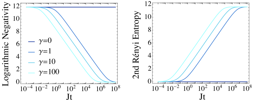
Figure 1: Logarithmic negativity and Rényi entropy of the stochastic SYK model. A log-linear plot of the (a) logarithmic negativity and (b) Rényi entropy (n=2) displayed as a function of time for different decoherence coefficients $\gamma$ in the stochastic SYK model with $N=26$ Majorana Fermions. The data is built from 100 independent samples and $\beta=1$.

We first consider the role of the open dynamics on the logarithmic negativity, an entanglement monotone defined as $E_{N}(\tilde{\rho}_{t})=\log_{2}\|\tilde{\rho}_{t}^{\Gamma_{L}}\|_{1}$ in terms of the trace norm of the partial transpose of the density matrix $\tilde{\rho}_{t}^{\Gamma_{L}}$, e.g., with respect to the left copy. Figure 1 shows that as a function of time this quantity exhibits a monotonic decay, signaling the loss of entanglement between the two copies of the TFD state. By contrast, $E_{N}(\tilde{\rho}_{t})$ remains constant under the unitary evolution with $\gamma=0$. The loss of entanglement is accompanied by information loss, manifested by the monotonic growth of the second Rényi entropy $S_{2}(\tilde{\rho}_{t})=-\log_{2}\mathrm{Tr}(\tilde{\rho}_{t}^{2})$ that stems exclusively from the nonunitary features of the dynamics encoded in the dissipator; see Fig. 1. Again, this quantity is invariant under unitary dynamics. The relevant time scale governing their evolution is the decoherence time that can be extracted from the short-time asymptotics of the purity, $P_{t}=\mathrm{Tr}(\tilde{\rho}_{t}^{2})$, which is invariant under unitary dynamics. The time scale $\tau_{D}$ governs its short-time asymptotics according to $P_{t}=1-t/\tau_{D}+\mathcal{O}(t^{2})$ Shimizu and Miyadera (2002); Beau et al. (2017); Xu et al. (2019). The same behavior, replacing $\tau_{D}$ by $2\tau_{D}$, rules the early decay of the fidelity due to the nonunitary character of the evolution, i.e., $F_{t}=1-t/({2\tau_{D}})+\mathcal{O}(t^{2})$ Lidar et al. (1998); Chenu et al. (2017). The time scale in which the TFD becomes diagonal in the energy eigenbasis is set by Xu et al. (2019)

$$\frac{1}{\tau_{D}}=4\gamma\frac{\mathrm{d}^{2}}{\mathrm{d}\beta^{2}}\ln\left[Z(\beta)\right].$$ (9)

Using a Gaussian approximation for the density of states $\varrho(E)$ at large $N$ García-García and Verbaarschot (2016, 2017); Liu et al. (2017), one finds $\tau_{D}=1/(\gamma N)$ SM . The monotonic decay of $E_{N}(\tilde{\rho}_{t})$ and $S_{2}(\tilde{\rho}_{t})$ prevents an investigation of the competition between quantum chaos signatures and information loss. To this end, we rely on the use of the fidelity $F_{t}$.

Under unitary evolution, the fidelity of the TFD state in the SYK model exhibits the typical features of chaotic quantum systems Cotler et al. (2017); Dyer and Gur-Ari (2017); del Campo et al. (2017), namely a decay, dip, ramp and plateau. The existence of a plateau is a consequence of the Hilbert space finite dimension, in which the energy spectrum is discrete. It is absent in systems with a continuous spectrum, where the decay is uninterrupted and continues to a vanishing value Fock and Krylov (1947); Beau et al. (2017). As a function of the time of evolution, the behavior of the fidelity is first dominated by (i) the density of states and decays from unity until it reaches a minimum value at a dip occurring at the dip time $t_{d}\sim\sqrt{d}$, where $d$ is the Hilbert space dimension of a single copy of the system. In the SYK, we estimate the dip time as

$$t_{d}\sim\left(\frac{\sqrt{\pi}\exp\left(-N\beta^{2}/4\right)}{c_{N}^{3/2}\sqrt{2N}}\right)^{1/4}\sqrt{d},$$ (10)

with $c_{N}$ a constant SM . The subsequent time evolution is dominated by correlations in the eigenvalue spacing and leads to (ii) a ramp that eventually saturates in (iii) a plateau with value $F_{p}=Z(2\beta)/Z(\beta)^{2}$ onset at the Heisenberg or plateau time $t_{p}\sim d$. Specifically, for the SYK model we find SM

$$t_{p}\simeq\alpha\sqrt{\frac{2\pi}{N}}d,$$ (11)

with $\alpha=2-\delta_{4,N\,\text{mod}\,8}$. This late stage is characterized by fluctuations around the plateau value, sometimes refer to as quantum noise in this context Barbón and Rabinovici (2014) to be distinguished from the kind of quantum noise that gives rise to decoherence Gardiner and Zoller (2004).

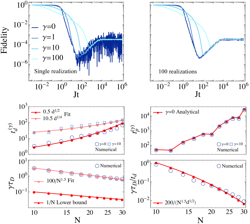
Figure 2: Fidelity of the stochastic SYK model. Top: A log-log plot of fidelity with different decoherence coefficients $\gamma$ in the SSYK model of $N=26$ Majorana Fermions. The data was taken by single and 100 independent samples and $\beta=1$. Bottom: The dip time $t_{d}^{(\gamma)}$, the plateau time $t_{p}^{(\gamma)}$, the decoherence time $\gamma\tau_{D}$, and $\gamma\tau_{D}$/$t_{d}$ are shown as a function of $N$.

The characteristic times $\tau_{D}$, $t_{d}$ and $t_{p}$ govern the competition between decoherence and quantum chaos.

Figure 2 shows the evolution of the fidelity for a finite-temperature TFD in a single realization and the disorder average over $J_{klmn}$. As the dephasing strength $\gamma$ is increased, the features of the fidelity $F_{t}$ manifested in the unitary case are gradually washed out. Prominently, for large dephasing strengths, $\tau_{D}\ll t_{p}$, the existence of the dip and ramp are completely suppressed and the fidelity decays monotonically from unit value towards the asymptotic one $F_{p}$. Between these extremes, the features that are more sensitive to information loss are those associated with quantum noise, e.g., the dynamical phase accumulated by the total Hamiltonian.

Under unitary dynamics, these fluctuations are exhibited around the dip and at long times: The decay towards the dip is typically characterized by a power-law given that the density of states is bounded from below, i.e., the existence of a ground state del Campo et al. (2017) (while this effect can be removed by smooth spectral filtering Šuntajs et al. (2019)). As a precursor of the dip, an oscillatory behavior is often present that can be understood as the interference of the power-law contribution and the ramp contribution stemming from correlations in the level spacing distribution. Whenever $\tau_{D}\leq t_{d}$, information loss leads to the suppression of these fluctuations. Regarding the presence of quantum noise at long times, whenever $\tau_{D}<t_{p}$, equation (5) shows that information loss associated with decoherence suppresses the fluctuations around the plateau value $F_{p}$. Importantly, the suppression of quantum noise fluctuations is already manifest at the level of a single realization of the SYK Hamiltonian, without averaging over $J_{klmn}$ or ensembles of system Hamiltonians. As shown in SM the behavior of the SYK models is in qualitative agreement with that of random-matrix ensembles. While under unitary dynamics this correspondence is only established at long times, its onset is facilitated by the presence of information loss. The decoherence time $\tau_{D}$ scales with $1/\gamma$ and the inverse energy variance. It thus decreases with temperature and the system size, as shown for the SYK in Fig 2. In the presence of information loss, the dip not only becomes shallower, but it shifts to later times; see Fig 2. For moderate values of the dephasing strength $\gamma$ the subsequent ramp is essentially unaffected with respect to the unitary dynamics, beyond the suppression of quantum noise. The time scale $t_{p}$ in which the plateau appears remains essentially constant. Thus, the ramp and plateau are shared by isolated and decohering systems exhibiting information loss.

Discussion and summary.— An experimental test of the interplay between quantum chaos and decoherence can be envisioned given advances in the quantum simulation of open systems by digital methods Barreiro et al. (2011) and tailored noise. It could be probed via the quantum simulation of the SYK Hamiltonian Danshita et al. (2017); García-Álvarez et al. (2017); Babbush et al. (2019); Luo et al. (2019) but it is generally expected in an arbitrary quantum chaotic system. While the preparation of the TFD state is being pursued Cottrell et al. (2019); Wu and Hsieh (2019); Zhu et al. (2019); Miceli and McGuigan (2019) this requirement can be relaxed for the study of some observables, such as the fidelity of a TFD state, as its expectation value can be related to that of a coherent Gibbs state $|\psi_{\beta}\rangle=\sum_{n}e^{-\beta E_{n}/2}|n\rangle/\sqrt{Z(\beta)}$ involving a single copy of the system. Indeed, under unitary time evolution $F_{t}=|\langle\psi_{\beta}|\exp(-itH)\psi_{\beta}\rangle|^{2}=|Z(\beta+it)/Z(\beta)|^{2}$ that can be measured by single-qubit interferometry Peng et al. (2015). Its general time-evolution can be described by a quantum channel $\rho_{t}=\Lambda_{t}[|\psi_{\beta}\rangle\langle\psi_{\beta}|]$ and the fidelity between the initial state and its evolved form is analogously given by $F_{t}=\langle\psi_{\beta}|\rho_{t}|\psi_{\beta}\rangle$. The measurement of the later can be simplified using quantum algorithms for the estimation of state overlaps Cincio et al. (2018); Cerezo et al. (2020).

In summary, the ubiquity of noise sources gives rise to a competition between the signatures of quantum chaotic dynamics expected for a many-body system in isolation and the presence of information loss resulting from decoherence. Such competition can be quantified by the fidelity between a thermofield state at a given time and its subsequent time evolution. For a quantum chaotic system in isolation this quantity equals the spectral form factor showing a dip-ramp-plateau structure which is suppressed by the loss of information induced by decoherence. The interplay between information loss and scrambling in open quantum complex systems should find broad applications in quantum computation, simulation and machine learning in the presence of noise.

Acknowledgements.— It is a pleasure to acknowledge discussions with Julian Sonner, Tadashi Takayanagi, and Jacobus Verbaarschot. TP acknowledges support by ERC Advanced grant 694544 OMNES and the program P1-0402 of Slovenian Research Agency. This work is further supported by ID2019-109007GA-I00.

Appendix A I. Fidelity in terms of spectral form factor

We start with the expression of the fidelity in Eq. (5), and use the Hubbard–Stratonovich transformation

$$e^{-\gamma t(E_{m}-E_{n})^{2}}=\frac{1}{2\sqrt{\pi\gamma t}}\int_{-\infty}^{+\infty}dye^{-\frac{y^{2}}{4\gamma t}}e^{-iy(E_{m}-E_{n})},$$ (S1)

to obtain a universal expression related to the normalized spectral form factor. The fidelity with Eq. (S1) is of the form

$$F_{t} = \frac{1}{2\sqrt{\pi\gamma t}}\int_{-\infty}^{+\infty}dye^{-\frac{y^{2}}{4\gamma t}}\frac{1}{Z^{2}(\beta)}\sum_{m,n}e^{-(\beta+2it+iy)E_{m}}e^{-(\beta-2it-iy)E_{n}}$$ (S2)

$$= \frac{1}{2\sqrt{\pi\gamma t}}\int_{-\infty}^{+\infty}dye^{-\frac{y^{2}}{4\gamma t}}\frac{\left|Z\left(\beta+2it+iy\right)\right|^{2}}{Z^{2}(\beta)}.$$

By changing the variable $\tau=y+2t$, Eq. (S2) can be further simplified to

$$F_{t}=\frac{1}{2\sqrt{\pi\gamma t}}\int_{-\infty}^{+\infty}d\tau e^{-\left(\frac{\tau-2t}{2\sqrt{\gamma t}}\right)^{2}}g_{\beta}(\tau),\text{ }$$ (S3)

with the spectral form factor

$$g_{\beta}(\tau)\equiv\frac{\left|Z\left(\beta+i\tau\right)\right|^{2}}{Z^{2}(\beta)},$$ (S4)

which is the expression given in Eq. (6) of the main text.

Appendix B II. Logarithmic negativity and the second Rényi entropy

The logarithmic negativity is defined as

$$E_{N}(\tilde{\rho}_{t})=\log_{2}\left\|\tilde{\rho}_{t}^{\Gamma_{L}}\right\|_{1},$$ (S5)

in terms of the trace norm of the partial transpose of the density matrix, while the second Rényi entropy is

$$S_{2}(\tilde{\rho}_{t})=-\log_{2}\mathrm{tr}\tilde{\rho}_{t}^{2}.\quad$$ (S6)

If the initial state is the thermal field double state, i.e.,

$$\tilde{\rho}_{0}=|\mathrm{TFD}\rangle\langle\mathrm{TFD}|=\frac{1}{Z(\beta)}\sum_{k,\ell}e^{-\frac{\beta}{2}(E_{k}+E_{\ell})}|k\rangle|k\rangle\langle\ell|\langle\ell|,$$ (S7)

the above Eqs. (S5) and (S6) can be written as

$$E_{N}(\tilde{\rho}_{t})=\log_{2}\left[\frac{1}{Z(\beta)}\sum_{k\ell}e^{-\beta(E_{k}+E_{\ell})/2-\gamma t(E_{k}-E_{\ell})^{2}}\right],$$ (S8)

and

$$S_{2}(\tilde{\rho}_{t})=-\log_{2}\left(P_{t}\right)\text{ with }P_{t}=\frac{1}{Z(\beta)^{2}}\sum_{k,\ell}e^{-\beta(E_{k}+E_{\ell})-2\gamma t(E_{k}-E_{\ell})^{2}}.$$ (S9)

Then we have

$$E_{N}(\tilde{\rho}_{t}(2\beta,2\gamma))+S_{2}(\tilde{\rho}_{t}(\beta,\gamma))=\log_{2}\frac{Z(\beta)^{2}}{Z(2\beta)}.$$ (S10)

Thus, the growth of the logarithmic negativity implies the decay of the second Rényi entropy, and viceversa, i.e., $\dot{E}_{N}(\tilde{\rho}_{t}(2\beta,2\gamma))=-\dot{S}_{2}(\tilde{\rho}_{t}(\beta,\gamma))$.

Appendix C III. Fidelity in terms of density of states and form factor

In what follows, we make explicit the connection between the fidelity, the density of states and the spectral form factor. The density of states is defined as

$$\varrho(E)=\sum_{n}N_{n}\delta(E-E_{n}),$$

where $N_{n}$ denotes the degeneracy of the energy level $E_{n}$.

The thermal state of a single copy can be written as

$$\rho_{\rm th}=\frac{1}{Z(\beta)}\int dE\sigma(E)e^{-\beta E}|E\rangle\langle E|.$$

Its purification is given by the thermofield double state

$$|\Psi\rangle=\frac{1}{\sqrt{Z(\beta)}}\int dE\sqrt{\varrho(E)}e^{-\beta E/2}|E,E\rangle.$$

The initial density matrix associated with the thermofield double state can then be written using a basis of continuous energy eigenstates as

$$\tilde{\rho}_{0}(E,E^{\prime})=\int dEdE^{\prime}\frac{e^{-\beta(E+E^{\prime})/2}}{Z(\beta)}\sqrt{\varrho(E)\varrho(E^{\prime})}|E,E\rangle\langle E^{\prime},E^{\prime}|.$$

In turn, the time-evolved density matrix reads

$$\tilde{\rho}_{t}(E,E^{\prime}) = \int dEdE^{\prime}\frac{e^{-\beta(E+E^{\prime})/2}}{Z(\beta)}\sqrt{\varrho(E)\varrho(E^{\prime})}e^{-2it(E-E^{\prime})}e^{-\gamma t(E-E)^{\prime 2}/2}|E,E\rangle\langle E^{\prime},E^{\prime}|$$ (S11)

$$= \sqrt{\frac{1}{4\pi\gamma t}}\int dEdE^{\prime}\int_{-\infty}^{\infty}dye^{-\frac{y^{2}}{4\gamma t}}\frac{e^{-\beta(E+E^{\prime})/2}}{Z(\beta)}\sqrt{\varrho(E)\varrho(E^{\prime})}e^{-2it(E-E^{\prime})}e^{-iy(E-E^{\prime})}|E,E\rangle\langle E^{\prime},E^{\prime}|$$ (S12)

and the fidelity becomes

$$F_{t}=\sqrt{\frac{1}{4\pi\gamma t}}\int_{-\infty}^{\infty}dye^{-\frac{y^{2}}{4\gamma t}}\frac{1}{Z(\beta)^{2}}\left|\int dE\sigma(E)e^{-(\beta-2it+iy)E}\right|^{2}.$$

The evaluation of such expression generally requires the use of numerical methods due to the lack of techniques to evaluate the average of the quotient of partition functions, each of which involving the Hamiltonian over which the average is performed. Under the annealed approximation, this average is approximated by the quotient of the averages. This approximation is generally valid at high temperature and fails at low temperature. Using it, the average fidelity reads

$$\langle F_{t}\rangle=\sqrt{\frac{1}{4\pi\gamma t}}\int_{-\infty}^{\infty}dye^{-\frac{y^{2}}{4\gamma t}}\frac{1}{\langle Z(\beta)^{2}\rangle}\int dEdE^{\prime}e^{-\nu(y)E-\bar{\nu}(y)E^{\prime}}\langle\varrho^{(2)}(E,E^{\prime})\rangle,$$

where

$$\nu(y)=\beta-2it+iy,\quad\bar{\nu}(y)=\beta+2it-iy.$$

The two-level correlation function $\langle\varrho^{(2)}(E,E^{\prime})\rangle=\langle\varrho(E)\varrho(E^{\prime})\rangle$ can be expressed in terms of the connected two-level correlation function $\langle\varrho_{c}^{(2)}(E,E^{\prime})\rangle$

$$\langle\varrho_{c}^{(2)}(E,E^{\prime})=\langle\varrho(E,E^{\prime})\rangle-\langle\varrho(E)\rangle\langle\varrho(E^{\prime})\rangle.$$

Assuming no degeneracies

$$F_{t}=\frac{G(\beta)}{Z(\beta)^{2}}+\frac{1}{Z(\beta)^{2}}\sum_{k\neq\ell}e^{-\beta(E_{k}+E_{\ell})+i2t(E_{k}-E_{\ell})-\gamma t(E_{k}-E_{\ell})^{2}}.$$ (S13)

where

$$G(\beta)=\sum_{n}N_{n}^{2}e^{-2\beta E_{n}}=\int dE\langle\varrho^{(2)}(E,E)\rangle e^{-2\beta E},$$

reduces to $Z(2\beta)$ in the absence of degeneracies expected for chaotic systems, i.e., when $N_{n}=1$.

Appendix D IV. Ensemble average of the fidelity

The ensemble average over the fidelity of Eq. (6) in the main text can be written as

$$\left\langle F_{t}\right\rangle=\frac{1}{2\sqrt{\pi\gamma t}}\int_{-\infty}^{+\infty}d\tau e^{-\left(\frac{\tau-2t}{2\sqrt{\gamma t}}\right)^{2}}\left\langle g_{\beta}(\tau)\right\rangle,\text{ }$$ (S14)

where the averaged spectral form factor in terms of annealing approximation is given by

$$\left\langle g_{\beta}(\tau)\right\rangle\doteq\frac{\left\langle\left|Z\left(\beta+i\tau\right)\right|^{2}\right\rangle}{\left\langle Z(\beta)\right\rangle^{2}}.$$ (S15)

Note that the annealing approximation is valid at high temperature (also see discussions in the end of Sec. V-A).

The density of states is defined as

$$\varrho(E)=\sum_{n}N_{n}\delta(E-E_{n}),$$

where $N_{n}$ denotes the degeneracy of the energy level $E_{n}$. Then the denominator and numerator of Eq. (S15) can be written as

$$\left\langle Z(\beta)\right\rangle=\int dE\langle\varrho(E)\rangle e^{-\beta E},$$ (S16)

and

$$\left\langle\left|Z\left(\beta+i\tau\right)\right|^{2}\right\rangle=\int dE\langle\varrho(E)^{2}\rangle e^{-2\beta E}+\int dEdE^{\prime}\langle\varrho(E)\varrho(E^{\prime})\rangle e^{-(\beta+i\tau)E}e^{-(\beta-i\tau)E^{\prime}},$$ (S17)

where the two-point correlation function can be expressed as

$$\langle\varrho(E)\varrho(E^{\prime})\rangle=\langle\varrho_{c}^{(2)}(E,E^{\prime})\rangle+\left\langle\varrho(E)\right\rangle\langle\varrho(E^{\prime})\rangle,$$ (S18)

in terms of the connected two-point correlation function $\varrho_{c}(E,E^{\prime})$.

In the following, we consider two examples, one is the GUE, and the other is the SYK model.

D.1 A. GUE-averaged Fidelity

For GUE ensembles, there are no degeneracy of the energy levels, so Eq. (S17) can be further written as

$$\left\langle\left|Z\left(\beta+i\tau\right)\right|^{2}\right\rangle_{\mathrm{GUE}}=\left\langle Z(2\beta)\right\rangle_{\mathrm{GUE}}+\left|\left\langle Z(\beta+i\tau)\right\rangle_{\mathrm{GUE}}\right|^{2}+\left\langle g_{\beta}^{c}(\tau)\right\rangle_{\text{{GUE}}},$$ (S19)

where

$$\left\langle g_{\beta}^{c}(\tau)\right\rangle_{\text{{GUE}}}=\int dEdE^{\prime}\langle\varrho_{c}^{(2)}(E,E^{\prime})\rangle_{\mathrm{GUE}}e^{-(\beta+i\tau)E}e^{-(\beta-i\tau)E^{\prime}}.$$ (S20)

The joint probability density of $H\in$GUE is proportional to $\exp(-\frac{1}{2\sigma^{2}}\mathrm{tr}H^{2})$, where $\sigma$ is the standard deviation of the random (off-diagonal) matrix elements of $H$. Note that in Ref. Mehta (2004), $\sigma=1/\sqrt{2}$, and in Ref. Cotler et al. (2017), $\sigma=1/\sqrt{d}$. To calculate Eq. (S19), we have to know the spectral density and the two-point correlation function. The eigenvalue density averaged over GUE is given by

$$\left\langle\varrho(E)\right\rangle_{\mathrm{GUE}}=\frac{1}{\sqrt{2}\sigma}K_{d}\left(\tilde{E},\tilde{E}\right),\text{ and }\tilde{E}:=\frac{E}{\sqrt{2}\sigma}\text{,}$$ (S21)

with the kernel $K_{d}(x,y)$ defined by

$$K_{d}(x,y)=\sum_{l=0}^{d-1}\phi_{l}(x)\phi_{l}(y)\text{, and }\phi_{l}(x):=\frac{e^{-\frac{x^{2}}{2}}\mathrm{H}_{l}(x)}{\sqrt{\sqrt{\pi}2^{l}l!}},$$ (S22)

where $\mathrm{H}_{l}(x)$ are the Hermite polynomials. Furthermore, the two-point correlation function averaged over GUE takes the form

$$\langle\varrho(E,E^{\prime})\rangle_{\mathrm{GUE}}=\frac{1}{2\sigma^{2}}\det\left[\left(\begin{array}[]{ll}K_{d}(\tilde{E},\tilde{E})&K_{d}(\tilde{E},\tilde{E}^{\prime})\\ K_{d}(\tilde{E}^{\prime},\tilde{E})&K_{d}(\tilde{E}^{\prime},\tilde{E}^{\prime})\end{array}\right)\right],$$ (S23)

and thus the connected two-level correlation function averaged over GUE reads

$$\langle\varrho_{c}^{(2)}(E,E^{\prime})\rangle_{\mathrm{GUE}}=-\frac{1}{2\sigma^{2}}\left(K_{d}(\tilde{E},\tilde{E}^{\prime})\right)^{2}.$$ (S24)

According to the orthogonality of Hermite polynomials

$$\int dxe^{-(x+a)^{2}}\mathrm{H}_{k}(x)\mathrm{H}_{l}(x)\text{=}\sqrt{\pi}2^{p}p!(-2a)^{|k-l|}\mathrm{L}_{p}^{(|k-l|)}(-2a^{2})\text{, }$$ (S25)

where $\mathrm{L}_{n}^{(\alpha)}(\cdot)$ are the associated Laguerre polynomials, and $p$:=min{$k,l$}, the first two items of Eq. (S19) and the denominator of Eq. (S15) is expressed as

$$\left\langle Z(x)\right\rangle_{\mathrm{GUE}}=e^{\frac{\sigma^{2}x^{2}}{2}}\mathrm{L}_{d-1}^{(1)}\left(-\sigma^{2}x^{2}\right).$$ (S26)

By Eqs. (S24) and (S25), the third term of Eq. (S19) is

$$\left\langle g_{\beta}^{c}(\tau)\right\rangle_{\text{{GUE}}}=-e^{\sigma^{2}(\beta^{2}-\tau^{2})}\sum_{k,l=0}^{d-1}\frac{p!}{q!}\left(\sigma^{2}(\beta^{2}+\tau^{2})\right)^{|k-l|}\left|\mathrm{L}_{p}^{(|k-l|)}\left(-\sigma^{2}(\beta+i\tau)^{2}\right)\right|^{2},$$ (S27)

where $q:=$max{$k,l$}.

With Eqs. (S26) and (S27), the spectral form factor is finally obtained

$$\left\langle g_{\beta}(\tau)\right\rangle_{\text{{GUE}}}\doteq\frac{e^{\sigma^{2}\beta^{2}}\mathrm{L}_{d-1}^{(1)}\left(-4\sigma^{2}\beta^{2}\right)+e^{-\sigma^{2}\tau^{2}}\left[\left|\mathrm{L}_{d-1}^{(1)}\left(-\sigma^{2}\beta_{\tau}^{2}\right)\right|^{2}-\sum_{k,l=0}^{d-1}\frac{p!}{q!}\left(\sigma^{2}\left|\beta_{\tau}\right|^{2}\right)^{|k-l|}\left|\mathrm{L}_{p}^{(|k-l|)}\left(-\sigma^{2}\beta_{\tau}^{2}\right)\right|^{2}\right]}{\mathrm{L}_{d-1}^{(1)}\left(-\sigma^{2}\beta^{2}\right)^{2}},$$ (S28)

with $\beta_{\tau}:=\beta+i\tau$ for short. Note again, one should replace $\tau$ with $2t$ when directly analyzing the spectral form factor.

To have a rough estimation of the dip and plateau time, we will consider an approximated connected two-level correlation function of Eq. (S24) when the dimension of GUE is large, i.e.,

$$\langle\varrho_{c}^{(2)}(E,E^{\prime})\rangle_{\mathrm{GUE}}\simeq-\frac{1}{\pi^{2}}\left(\frac{\sin((E-E^{\prime})\sqrt{d}/\sigma)}{E-E^{\prime}}\right)^{2}.$$ (S29)

By defining new variables $r=E-E^{\prime}$ and $\omega=(E+E^{\prime})/2$, Eq. (S20) is given by

$$\left\langle g_{\beta}^{c}(t)\right\rangle_{\text{{GUE}}}\simeq-\frac{1}{\pi^{2}}\int d\omega e^{-2\beta\omega}\int_{-\infty}^{\infty}dr\left(\frac{\sin(r\sqrt{d}/\sigma)}{r}\right)^{2}e^{-2itr},$$ (S30)

where we have replaced $\tau$ with $2t$. The first integration is divergent. For estimation, the integration is replaced with

$$\int d\omega\rightarrow\int_{-\omega_{0}}^{\omega_{0}}d\omega.$$ (S31)

Since the spectral density can be approximated by Wigner’s semicircle in large $d$ limit, i.e.,

$$\left\langle\varrho(E)\right\rangle_{\mathrm{GUE}}=\frac{\sqrt{d}}{\sigma\pi}\sqrt{1-\left(\frac{E}{2\sigma\sqrt{d}}\right)^{2}},\text{ and }|E|\leq 2\sigma\sqrt{d},$$ (S32)

thus $\left\langle\varrho(0)\right\rangle_{\mathrm{GUE}}=\sqrt{d}/(\sigma\pi)$. According to the normalization of $\left\langle\varrho(E)\right\rangle_{\mathrm{GUE}}$, we have $2\omega_{0}\left\langle\varrho(0)\right\rangle_{\mathrm{GUE}}\simeq d$, and

$$\omega_{0}\simeq\frac{\sigma\pi\sqrt{d}}{2},$$ (S33)

with which, the first integration reads

$$\int d\omega e^{-2\beta\omega}\simeq\frac{\sinh\left(\sqrt{d}\pi\beta\sigma\right)}{\beta}.$$ (S34)

The second integration in Eq. (S30) is the Fourier transform

$$\int_{-\infty}^{\infty}dr\left(\frac{\sin(r\sqrt{d}/\sigma)}{r}\right)^{2}e^{-2itr}=\left\{\begin{array}[]{ll}\pi(\sqrt{d}/\sigma-t),&t\leq\sqrt{d}/\sigma,\\ 0,&t>\sqrt{d}/\sigma.\end{array}\right.$$ (S35)

Equation (S30) finally takes the form

$$\left\langle g_{\beta}^{c}(t)\right\rangle_{\text{{GUE}}}\simeq\left\{\begin{array}[]{ll}-\frac{\sinh\left(\sqrt{d}\pi\beta\sigma\right)}{\pi\beta}(\sqrt{d}/\sigma-t),&t\leq\sqrt{d}/\sigma,\\ 0,&t>\sqrt{d}/\sigma.\end{array}\right.$$ (S36)

According to the above equation, it is easy to observe that the plateau time is

$$t_{p}=\sqrt{d}/\sigma.$$ (S37)

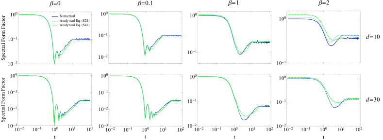
Figure S1: Spectral form factor of GUE. Analytical Eqs. (S28) and (S41) are in comparison with numerical calculations for $\beta=0,$ $0.1$, $1$, $2$, and $d=10$, $30$. The standard deviation of the random variables of $H$ is selected as $\sigma=1/\sqrt{d}$. The numerical calculations use 1000 independent realizations.

With Wigner’s semicircle law of Eq. (S32), the partition function averaged over the GUE ensembles is approximated by

$$\left\langle Z(x)\right\rangle_{\mathrm{GUE}}=\frac{\sqrt{d}\mathrm{I}_{1}(2\sigma\sqrt{d}x)}{\sigma x},$$ (S38)

where $\mathrm{I}_{n}(\cdot)$ is the modified Bessel function of first kind and order $n$. When $\beta\ll 1$ and $t$ is large, the asymptotic expansion of the second part of Eq. (S19) reads

$$\left|\left\langle Z(\beta+i2t)\right\rangle_{\mathrm{GUE}}\right|^{2}\simeq\frac{\sqrt{d}(1-\sin(8\sigma\sqrt{d}t))}{16\pi t^{3}\sigma^{3}}.$$ (S39)

By equating Eq. (S39) and Eq. (S36), the dip time can be estimated as

$$t_{d}\simeq\frac{1}{2}\left(\frac{\sqrt{d}\beta}{\sigma^{3}\sinh\left(\sqrt{d}\pi\beta\sigma\right)}\right)^{\frac{1}{4}}\simeq\frac{1}{2\pi^{1/4}\sigma}-\frac{d\pi^{7/4}\sigma}{48}\beta^{2}+\mathcal{O}(\beta^{3}).$$ (S40)

The spectral form factor in the large $d$ limit is obtained

$$\left\langle g_{\beta}(t)\right\rangle_{\text{{GUE}}}\simeq\frac{\frac{\sqrt{d}\mathrm{I}_{1}(4\sigma\sqrt{d}\beta)}{2\sigma\beta}+\frac{\sqrt{d}(1-\sin(8\sigma\sqrt{d}t))}{16\pi t^{3}\sigma^{3}}+\text{Eq}.(\ref{gc4})}{\left(\frac{\sqrt{d}\mathrm{I}_{1}(2\sigma\sqrt{d}\beta)}{\sigma\beta}\right)^{2}}.$$ (S41)

In Fig. (S1), the spectral form factor with Eqs. (S28), and (S41) are compared with the numerical calculations. Note that when the dimension $d$ increases, the valid domain of $\beta$ by annealing approximation becomes larger.

D.2 B. Spectral form factor of the SYK model

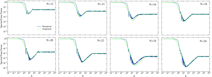
Figure S2: Spectral form factor of SYK model. Analytical Eq. (S52) is commpared with numerical calculations ($\beta=0.1$).

For SYK model with $N$ mod $8\neq 0$, the energy spectrum has a uniformly double degeneracy ($N_{n}=2$). Equation (S17) can be written as

$$\left\langle\left|Z\left(\beta+i2t\right)\right|^{2}\right\rangle_{\mathrm{SYK}}=2\left\langle Z(2\beta)\right\rangle_{\mathrm{SYK}}+\left|\left\langle Z(\beta+i2t)\right\rangle_{\mathrm{SYK}}\right|^{2}+\left\langle g_{\beta}^{c}(t)\right\rangle_{\text{{SYK}}},$$ (S42)

where

$$\left\langle g_{\beta}^{c}(\tau)\right\rangle_{\text{{SYK}}}=\int dEdE^{\prime}\langle\varrho_{c}(E,E^{\prime})\rangle_{\mathrm{SYK}}e^{-(\beta+2ti)E}e^{-(\beta-2ti)E^{\prime}}.$$ (S43)

To calculate the first two items of Eq. (S42), we need to know the spectral density of the SYK model, which has been derived by the method of moments

$$\left\langle\varrho(E)\right\rangle_{\mathrm{SYK}}=\frac{1}{2\pi}\int dte^{-iEt}\left\langle\text{Tr}(e^{iHt})\right\rangle_{\mathrm{SYK}}.$$ (S44)

In this part, we are going to roughly estimate the dip and plateau time, therefore, the spectral density can be approximated in a Gaussian type when $N$ is large García-García and Verbaarschot (2016, 2017); Liu et al. (2017)

$$\left\langle\varrho(E)\right\rangle_{\mathrm{SYK}}\simeq\sqrt{\frac{2}{\pi N}}d\exp\left(-\frac{2E^{2}}{N}\right).$$ (S45)

The partition function is

$$\left\langle Z(x)\right\rangle_{\mathrm{SYK}}\simeq d\exp\left(\frac{Nx^{2}}{8}\right).$$ (S46)

With such equation, the decoherence time can be estimated by

$$\gamma\tau_{D}\geq\frac{1}{4\frac{\mathrm{d}^{2}}{\mathrm{d}\beta^{2}}\ln\left[\left\langle Z(\beta)\right\rangle_{\mathrm{SYK}}\right]}=\frac{1}{N}.$$ (S47)

Since the late time behavior of the SYK model is governed by GOE, GUE, and GSE statistics according to the number of Majorana Fermions modulo $8$. For simplicity, we first consider the connected part of the two-point correlation function of GUE (i.e., $N$ mod $8=2$ or $6$) as

$$\langle\varrho_{c}^{(2)}(E,E^{\prime})\rangle_{\mathrm{SYK}}\simeq-\left(\frac{\sin(2\pi r\left\langle\varrho(\omega)\right\rangle_{\mathrm{SYK}})}{\pi r}\right)^{2},$$ (S48)

with $r=E-E^{\prime}$ and $\omega=(E+E^{\prime})/2$ defined in above subsection. Then

$$\left\langle g_{\beta}^{c}(t)\right\rangle_{\text{{SYK}}} \simeq \int dEdE^{\prime}\langle\varrho_{c}(E,E^{\prime})\rangle_{\mathrm{SYK}}e^{-(\beta+2it)E}e^{-(\beta-2it)E^{\prime}},$$ (S51)

$$= -\int d\omega e^{-2\beta\omega}\int dr\left(\frac{\sin(2\pi r\left\langle\varrho(\omega)\right\rangle_{\mathrm{SYK}})}{\pi r}\right)^{2}e^{-irt},$$

$$= \left\{\begin{array}[]{ll}\frac{\sqrt{N}\left\langle Z(2\beta)\right\rangle_{\mathrm{SYK}}}{\sqrt{2\pi}d}t-2\left\langle Z(2\beta)\right\rangle_{\mathrm{SYK}},&t\lesssim 2\sqrt{\frac{2\pi}{N}}d,\\ 0,&t>2\sqrt{\frac{2\pi}{N}}d.\end{array}\right.$$

With Eqs. (S46) and (S51), the spectral form factor of the SYK reads

$$\left\langle g_{\beta}(t)\right\rangle_{\text{{SYK}}}\simeq\frac{\left|\left\langle Z(\beta+i2t)\right\rangle_{\mathrm{SYK}}\right|^{2}}{\left\langle Z(\beta)\right\rangle_{\mathrm{SYK}}^{2}}+\left\{\begin{array}[]{ll}\frac{\sqrt{N}}{2\sqrt{2\pi}d}\left\langle g_{\beta}(\infty)\right\rangle_{\text{{SYK}}}t,&t\lesssim 2\sqrt{\frac{2\pi}{N}}d,\\ \left\langle g_{\beta}(\infty)\right\rangle_{\text{{SYK}}}&t>2\sqrt{\frac{2\pi}{N}}d,\end{array}\right.$$ (S52)

where $\left\langle g_{\beta}(\infty)\right\rangle_{\text{{SYK}}}$ is the spectral form factor in the long time limit

$$\left\langle g_{\beta}(\infty)\right\rangle_{\text{{SYK}}}=\frac{2\left\langle Z(2\beta)\right\rangle_{\mathrm{SYK}}}{\left\langle Z(\beta)\right\rangle_{\mathrm{SYK}}^{2}}\simeq\frac{2}{d}\exp\left(\frac{N\beta^{2}}{4}\right).$$ (S53)

Note that when $N$ mod $8=0$, i.e., the GOE case, there is no degeneracy, and the plateau height would be $\exp\left(N\beta^{2}/4\right)/d$. From Eq. (S52), the plateau time is given by

$$t_{p}\simeq 2\sqrt{\frac{2\pi}{N}}d.$$ (S54)

For GOE ($N$ mod $8=0$) and GSE ($N$ mod $8=4$), the calculations would become rather lengthy. Since we only aim to roughly estimate the time scale, we still use the GUE, and modified the plateau time according to the numerical results. For GSE, the plateau time is around $t_{p}\simeq\sqrt{2\pi/N}d$. Unlike the GUE and GSE, the ramp and plateau connect smoothly for the GOE, so it is hard to strictly define the plateau time, for simplicity, we still use Eq. (S54) for estimation.

Before the dip time, the edges of the spectrum cannot be omitted, thus Eq. (S46) is no longer applicable. Thus, we will replace it with $\left\langle Z(x)\right\rangle_{\mathrm{SYK}}\simeq x^{-3/2}$ García-García and Verbaarschot (2016, 2017); Cotler et al. (2017), and the first part of Eq. (S52) is given by

$$\frac{\left|\left\langle Z(\beta+i2t)\right\rangle_{\mathrm{SYK}}\right|^{2}}{\left\langle Z(\beta)\right\rangle_{\mathrm{SYK}}^{2}}\simeq\frac{\beta^{3}}{(\beta^{2}+c_{N}t^{2})^{3/2}},$$ (S55)

with $c_{N}\simeq N/400$ fitted by numerical calculations. Then, the dip time is roughly estimated as

$$t_{d}\sim\left(\frac{\sqrt{\pi}\exp\left(-N\beta^{2}/4\right)}{c_{N}^{3/2}\sqrt{2N}}\right)^{1/4}\sqrt{d}\varpropto\sqrt{d}.$$ (S56)

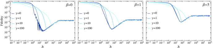
Figure S3: Fidelity of the stochastic SYK model for different temperatures. A log-log plot of the fidelity of SSYK model ($N=26$) under different temperature. The variation of the temperature has a negligible effect on the dip and plateau time.

Although Eqs. (S54) and (S56) are derived when $\beta$ is small, they are still valid for low temperature for estimation, just as shown in Fig. (S3).