The Projected Belief Network Classfier : both Generative and Discriminative.

Abstract

The projected belief network (PBN) is a layered generative network with tractable likelihood function, and is based on a feed-forward neural network (FF-NN). It can therefore share an embodiment with a discriminative classifier and can inherit the best qualities of both types of network. In this paper, a convolutional PBN is constructed that is both fully discriminative and fully generative and is tested on spectrograms of spoken commands. It is shown that the network displays excellent qualities from either the discriminative or generative viewpoint. Random data synthesis and visible data reconstruction from low-dimensional hidden variables are shown, while classifier performance approaches that of a regularized discriminative network. Combination with a conventional discriminative CNN is also demonstrated.

I Introduction

I-A Background and Motivation

Much has been published on the comparison of generative and discriminative classifiers. The widespread view is that discriminative classifiers generalize better when sufficient labeled training data is available [1]. Despite their success, it has been recognized that discriminative methods have flaws, vividly demonstrated by adversarial sampling [2], a technique in which small, almost imperceptible changes to the input data cause false classifications. Because generative classifiers are based on a model of the underlying data distribution, they are less succeptible to adversarial sampling and can complement discriminative classifiers. There are a large number of methods that seek to combine generative and discriminative classifiers [3, 4, 5, 6, 7, 8, 1], or to combine discriminative and generative training [1, 9, 10]. The weakness of generative classifiers stems from the need to estimate the data distribution, a very difficult task that is unecessary when just classifying between known data classes [11]. In modeling complex data generation processes found in real-world data, traditional probability density function (PDF) estimators such as kernel mixtures and hidden Markov models do not suffice. Deep layered generative networks (DLGNs) can model complex generative processes, but the data distribution, also called likelihood function (LF) is intractable, complicating training and inference. Reason: the hidden variables are jointly distributed with the input data and must be integrated out. Such networks need to be trained using surrogate cost functions such as contrastive divergence to train restricted Boltzmann machines [12, 13], and Kullback Leibler divergence to train variational auto-encoder (VAE) [14], or an adversarial discriminative network to train generative adversarial networks (GAN) [15]. Using DLGNs as classifiers is problematic not just because of the intractability of the LF, but because the performance of generative models in general lags behind discriminative classifiers. Significant performance improvements could potentially be made by combining DLGNs with deep discriminative networks. But, in order to see a benefit by combining, all classifiers need to have good performance. Therefore, having a DLGN classifier with comparable performance to deep discriminative network would be greatly desireable. In summary, there is a need for a DLGN with tractable LF that can be combined with discriminative approaches. The newly introduced layered generative network called projected belief network (PBN) stands out as a potentially better choice to achieve these goals. The PBN is a DLGN, so can model complex generative processes, but stands out from all other DLGNs. The tractable LF allows direct gradient training and enables detection of out-of-set samples (outliers that are outside of the set of training classes). Because the PBN is based on a feed-forward neural network (FF-NN), it can share an embodiment with a discriminative classifier (i.e. it is a single network that is both a complete generative model and a discriminative classifier), so is a more direct way to introduce the advantages of generative models into a discriminative classifier, or vice-versa.

I-B Main Idea

The PBN is based on a feed-forward neural network (FF-NN). Figure 1 shows a simple 3-layer FF-NN.

Figure 1: A feed-forward neural network (FF-NN). This FF-NN can be a discriminative classifier if $\lambda_{4}$ is the softmax function and the output box is the cross-entropy cost function. It can also be a generative model if viewed as PBN and the output box is the output prior distribution $g({\bf x}_{4})$.

Each layer $l$ consists of a linear transformation (represented by matrix ${\bf W}_{l}$), a bias ${\bf b}_{l}$ and an activation function $\lambda_{l+1}(\;)$. The linear transformation can be fully-connected or convolutional, but must have total output dimension equal to or lower than the input dimension. This network can serve as a traditional classifier network if the output layer dimension is equal to the number of classes (and the final activation function is softmax). On the other hand, it can also be viewed as a projected belief network (PBN) [16, 17] whose properties are reviewed below.

I-C Mathematical Foundation

Suppose we are given a fixed dimension-reducing transformation mapping high-dimensional input data ${\bf x}\in\mathbb{R}^{N}$ to a lower-dimensional feature ${\bf z}\in\mathbb{R}^{M}$, $M<N$, denoted by ${\bf z}=T({\bf x})$. If the probability density function (PDF) of the feature, denoted by $g({\bf z})$, is estimated or specified, then we may ask the question “given $g({\bf z})$ and $T({\bf x})$, what is a good estimate of the PDF of ${\bf x}$?”. The method of maximum entropy (MaxEnt) PDF projection [18] finds a unique PDF defined on $\mathbb{R}^{N}$ with highest entropy among all PDFs consistent with $T({\bf x})$ and $g({\bf z})$. When PDF projection is applied layer-wise to a feed-forward neural network (identified with $T({\bf x})$) then a projected belief network (PBN) results [16, 17]. The LF for the network in Figure 1 is given by (see [17])

$$\begin{array}[]{l}p_{p}({\bf x}_{1};T,g)=\frac{1}{\displaystyle\epsilon}\;\frac{\displaystyle p_{1}({\bf x}_{1})}{\displaystyle p_{1}({\bf z}_{1})}\;|{\bf J}_{{\bf z}_{1}{\bf x}_{2}}|\\ \;\;\;\;\;\;\;\;\;\cdot\;\frac{\displaystyle p_{2}({\bf x}_{2})}{\displaystyle p_{2}({\bf z}_{2})}\;|{\bf J}_{{\bf z}_{2}{\bf x}_{3}}|\;\frac{\displaystyle p_{3}({\bf x}_{3})}{\displaystyle p_{3}({\bf z}_{3})}\;|{\bf J}_{{\bf z}_{3}{\bf x}_{4}}|\;g({\bf x}_{4}),\end{array}$$ (1)

where $p_{l}({\bf x}_{l})$ is the assumed prior distribution for the input to layer $l$, $p_{l}({\bf z}_{l})$ is the distribution of ${\bf z}_{l}$ under the assumption that ${\bf x}_{l}$ is distributed according to $p_{l}({\bf x}_{l})$, $|{\bf J}_{{\bf z}_{l}{\bf x}_{l+1}}|$ is the determinant of the Jacobian (matrix of gradients) of the invertible transformation mapping ${\bf z}_{l}\rightarrow{\bf x}_{l+1}$, and where $g({\bf x}_{L+1})$ is the assumed prior for the output of a network. The constant $\epsilon$ is the sampling efficiency discussed below.

I-D PBN layers and MaxEnt Priors

The properties of PBN layer depend greatly on the assumed prior distribution $p_{l}({\bf x}_{l})$, which is selected using the principle of Maximum Entropy (MaxEnt) and depends on the assumed input data range for the layer [19]. Consider a generic PBN layer with input dimension $N$. There are three canonical input data ranges, unlimited denoted by $\mathbb{R}^{N}$, positive quadrant where $0<x_{i}$ denoted by $\mathbb{P}^{N}$, and the unit hypercube where $0<x_{i}<1$ denoted by $\mathbb{P}^{N}$. The MaxEnt priors for these data ranges are given in Table I. For each data range and prior, there is a prescribed input non-linearity (activation function) $\lambda(\;)$ which is also given in the table and should be applied at the output of the previous layer. The TG and TED activations resemble softplus and sigmoid, respectively [19]. Dimension-preserving layers are also possible ($M=N$) and are analyzed using the determinant of the Jacobian matrix of the transformation.

${\cal X}$	MaxEnt Prior $p_{0}({\bf x})$	$\lambda(\alpha)$
$\mathbb{R}^{N}$	$\prod_{i=1}^{N}{\cal N}(x_{i})$ (Gaussian)	$\alpha$ (Linear)
$\mathbb{P}^{N}$	$\prod_{i=1}^{N}2{\cal N}(x_{i}),\;\;0<x_{i}$ (TG)	$\alpha+\frac{{\cal N}(\alpha)}{\Phi(\alpha)}$ (TG)
$\mathbb{U}^{N}$	$1,\;\;0<x_{i}<1$ (Uniform)	$\frac{e^{\alpha}}{e^{\alpha}-1}-\frac{1}{\alpha}$ (TED)

TABLE I: MaxEnt priors and activation functions as a function of input data range. TG=“Trunc. Gauss.”. TED=“Trunc. Expon. Distr”. ${\cal N}\left(x\right)\stackrel{{\scriptstyle\mbox{\tiny$\Delta$}}}{{=}}\frac{e^{-x^{2}/2}}{\sqrt{2\pi}}$ and $\Phi\left(x\right)\stackrel{{\scriptstyle\mbox{\tiny$\Delta$}}}{{=}}\int_{-\infty}^{x}{\cal N}\left(x\right).$

The sampling efficiency $\epsilon$ is less than 1 if the output range of a layer is not identical to the assumed input range of the next layer resulting in subspace mismatch. However, $\epsilon$ is driven closer to 1 as the network trains [17], so can be ignored (i.e. assumed to be 1.0) for all practical purposes. It is also possible to create PBNs with sampling efficiency identically equal to 1 by using layers with Gaussian prior and dimension-preserving layers ($M=N$), both of which have no subspace mismatch. The PBN is trained by maximizing the mean of the log of (1) using stochastic gradient ascent.

II Technical Approach

II-A Output Non-Linearity and Prior

In order to create a PBN that is also a discriminative classifier, a label-dependent output non-linearity and output prior are required. A simple approach would be to apply a label-dependent level-shift to the output variables, then assume a zero-mean standard normal output prior. Specifically, one applies a level-shifting function $\lambda(z_{i})=z_{i}-l_{i}$, $1\leq i\leq M$, where $z_{i}$ is the network output (prior to activation function), where $M$ is the number of data classes and the dimension of the network output, and ${\bf l}=[l_{1},l_{2}\ldots l_{M}]$ is the label signal, a shifted one-hot encoding of the ground-truth label, with elements taking values of $-L$ or $L$. Then, training with the simple Gaussian prior $g({\bf x}_{L+1})={\cal N}({\bf x}_{L+1}),$ where ${\cal N}({\bf x})=-\frac{M}{2}\log(2\pi)-\frac{1}{2}{\bf x}^{\prime}{\bf x}$ encourages the network output to agree with the label signal. But, this approach makes little penalty for classification errors. The function

$$\lambda(z_{i})=z_{i}+C[\sigma(3z_{i})-.5]-l_{i}*(L+C/2)/L,$$

where $\sigma(\;)$ is the sigmoid function and $C$ is a large constant, produces a dynamic level shift that greatly increases if the network output has the wrong sign (compared to the label). When combined with the standard normal prior, it encourages Gaussian modes at -$L$ and +$L$, but imposes a very large penalty for class errors. The degree of discriminative training can be varied by changing $C$.

II-B MaxEnt Reconstruction and Synthesis

We now investigate a distinctly generative property of the PBN : visible data reconstruction from hidden variables. Input data can be randomly synthesized or reconstructed from the output of any layer of the FF-NN. Unlike other generative networks, the PBN is not an explicit generative network, it operates implicitly by “backing up” through a FF-NN. In each layer, the PBN selects a sample from the set

$${\cal M}({\bf z})=\{{\bf x}:{\bf W}^{\prime}{\bf z}={\bf x}\},$$

which is the set of samples ${\bf x}$ that “could have” produced ${\bf z}$. A sample is selected from ${\cal M}({\bf z})$ with probability density proportional to the prior distribution $p_{0}({\bf x})$. When $p_{0}({\bf x})$ is the uniform distribution, this is called uniform manifold sampling (UMS) [20]. Sampling requires a type of Markov chain Monte-Carlo (MCMC) [20]. Deterministic data generation is also possible if instead of randomly selecting a sample in ${\cal M}({\bf z})$, we select the mean (the conditional mean given ${\bf z}$) , denoted by $\hat{{\bf x}}|{\bf z}={\mathbb{E}}({\bf x}|{\bf z}).$ This can be found in closed form for a range of MaxEnt priors [19, 17, 20] and is given by $\hat{{\bf x}}|{\bf z}=\lambda({\bf W}\hat{{\bf h}}),$ where $\lambda(\;)$ is given in Table I and $\hat{{\bf h}}$ is the solution of the equation

$${\bf W}^{\prime}\lambda\left({\bf W}{\bf h}\right)={\bf z}.$$ (2)

This solution is guaranteed to exist as long as ${\bf x}$ is in the support $p_{0}({\bf x})$ and is also the saddle-point for the saddle-point approximation to $p_{0}({\bf z})$ [19]. For the simplest case of Gaussian MaxEnt prior, the activation function is linear, $\lambda(\alpha)=\alpha$, and the reconstruction is by least-squares, $\hat{{\bf x}}|{\bf z}={\bf W}\left({\bf W}^{\prime}{\bf W}\right)^{-1}{\bf z}.$

Starting at any layer output, one can proceed in the backward direction up the network, increasing the dimension, until the visible data is reconstructed. There are two possible reconstruction methods, (a) random sampling in ${\cal M}({\bf z})$ by MCMC, and (b) deterministically selecting the conditional mean $\hat{{\bf x}}|{\bf z}$. When subspace mismatch occurs, the reconstruction chain could fail. The rate of success is the sampling efficiency discussed above, and is different for stochastic and deterministic reconstruction. Generally, a trained network has a deterministic sampling efficiency of 1 (failure is rare or non-existent). Reconstructing from dimension-preserving layers involves just a matrix inversion, so has a sampling efficiency of 1. Layers with Gaussian input assumption also have a sampling efficiency of 1. Deep networks can be constructed using these two layer types to obtain deep PBNs with sampling efficiency of 1.

When only determintstic reconstruction is used, the result is a deterministic PBN [17], a type of auto-encoder where the reconstruction network that is defined by the analyis network.

II-C PBN Properties

The PBN differs significantly from other methods of combining the roles of generative and discriminative networks because the discriminative influence is added into the output prior and does not disturb the “purity” of the generative network. There is no compromise between generative and discriminative training or structure, they are both contained in one network and one cost function.

When reconstructing visible data from hidden variables, the synthesized data, when applied to the feed-forward network, produces exactly the same hidden variables as were created during the generation process. This property of hidden variable recovery is unique to the PBN.

During training, when the discriminative cost function is “satisfied” (the training data is almost completely separated), then the generative cost dominates, so the network becomes the best possible PBN that at the same time separates the data. This can be seen as a generative regularization effect.

III Classification of Spectrograms of Words Commands

III-A Data set

The data was selected to be at the same time relevant, realistic, and challenging. We selected a subset of the Google speech commands data [21], choosing three pairs of difficult to distinguish words: “three, tree”, “no, go”, and “bird, bed”, sampled at 16 kHz and segmented into into 48 ms Hanning-weighted windows shifted by 16 ms. We used log-MEL band energy features with 20 MEL-spaced frequency bands and 45 time steps, representing a frequency span of 8 kHz and a time span of 0.72 seconds. The input dimension was therefore $N=45\times 20=900.$ From each of the six classes, we selected 500 training samples, 150 validation samples, at random. The remaining samples were used to test, averaging about 1500 per class or about a total of 10000 testing samples.

III-B Network

A separate network was trained on each word pair. The networks had $L=5$ layers. The first layer was convolutional with 9 ($21\times 17$) convolutional kernels using “same” border mode and $5\times 4$ downsampling (not pooled, just down-sampled), thus producing 9 ($9\times 5$) output feature maps, or a total output dimension of 405. The second layer was convolutional with 24 ($5\times 3$) convolutional kernels using “same” border mode and $2\times 2$ downsampling, thus producing 24 ($3\times 2$) output feature maps, or a total output dimension of 144. The remaining two layers were fully-connected with 64, and 24 neurons. The output layer had 2 neurons, matching the number of classes. Note that we sought to reduce the dimension in each layer by at least a factor of 2. The layer output activation functions were linear, linear, TG, TG, and linear (See Table I).

III-C Classification Results

For a classifier benchmark, we trained a conventional CNN classifier network on each class pair. Each network consisted of seven layers, three convolutional and four dense layers. The convolutional layers had kernel shapes of $(11\times 5)$, $(7\times 5)$, and $(3\times 3)$, max-pooling of $(5\times 2)$, $(3\times 2)$, and $(1\times 1)$, with 64, 32, and 48 kernels, respectively. Soft-plus activation and “same” convolutional padding was used. The dense layers had 256, 128, 32 , and 2 neurons. Dropout and batch normalization were used with ADAM optimization. Classification accuracy for the CNN is given in Table II.

The PBN networks were first initialized with random weights and trained as a standard discriminative deep neural network (DNN) with dropout and L-2 regularization. No data augmentation (such as random shifting) was used. Classification accuracy for the initial PBNs is given in Table II as ‘PBN(DNN)”.

	”three-tree”	”no-go”	”bird-bed”
CNN	0.923	0.924	0.965
PBN(DNN)	0.873	0.859	0.960
PBN	0.886	0.863	0.960
PBN+CNN	0.925	.926	0.971

TABLE II: Classification accuracy for the three class pairs.

The initialized PBN were then trained as a PBN by maximizing the mean likelihood function (1) with output prior distribution parameter $C=200$ and L2 regularization. The classification results for the PBN on the three class pairs are shown in Table II where they can be compared with the initial DNN-trained networks “PBN(DNN)”. Note that the PBN has about the same accuracy as “PBN(DNN)”, with slightly higher accuracy for two class pairs. This demonstrates that the PBN training does not seem to impact the classifcation performance of a network, and may even help. Training a classifier network as a PBN can be regarded as a form of regularization.

III-D Reconstruction Results

It has been established that the PBN has lost little in terms of classification performance wwhen compared to the initial regularized discriminative networks. It will now be determined what has been gained in terms of generative power. The first thing that comes to mind is the reconstruction of visible data from the hidden variables. Using the method of Section II-B, we reconstructed data from the hidden variables of the first and second layer of the initial PBN “PBN(DNN)”, with dimensions 405 and 144, respectively. Results are shown in Figure 2.

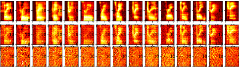
Figure 2: Samples of spoken word commands “three” and “tree” and reconstruction using the discriminatively-trained network. From top: original samples, first-layer reconstructions, second-layer reconstructions.

Little resemblance can be seen despite the high dimension of the hidden variables. This is how the network sees the data through the hidden variables. The noisy images, when used as input data will produce exactly the same hidden variables at the given layer as the original input sample, a disturbing fact that vividly illustrates one of the problems with discriminative networks.

The reconstruction experiment was repeated for the trained PBN. Results are shown in Figure 3.

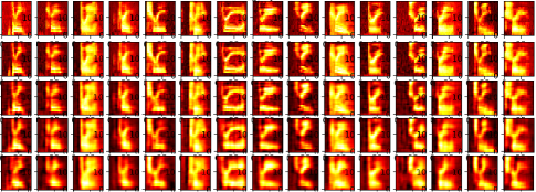
Figure 3: Samples of speech commands “three, three” reconstructed using PBN. From top: original spctrograms, then the same reconsructed from output of first through fourth layers, with hidden variable dimensions of 405, 144, 64, and 24, respectively.

This time, reconstruction was attempted from deep within the network. The reconstructions had excellent quality, but gradually decreasing sharpness. Note that this network was not trained for lower reconstruction error, but instead to maximize (1). The reconstruction power of the network comes as a side-effect and can be tapped into anywhere in the network.

III-E Classifying between class pairs

A second exercise in “generative capability” is the classification between class pairs using models trained separately on just one pair. This demonstrates the ability to recognize out-of set events. To classify between pairs, visible data reconstruction error was calculated based on the 24-dimensional output of the fourth layer (not using the output layer), and the model giving least error was chosen. Figure 4 shows the classifier statistic (negative log of mean square reconstruction error). The inter-pair classification accuracy was 87.9%, which is good considering the number of mal-formed events in the data base and that the models were separately trained, without access to data of the competing class pairs.

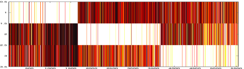
Figure 4: Classifier statistic (negative log of mean square reconstruction error) for classifying between class pairs based on reconstruction error.

III-F Combination with CNN

We have postulated above that having a generative classifier with comparable performance to a discriminative one would allow for performance gains when combining them. To demonstrate this, the PBN was combined with the CNN benchmark classifier described above. In Figure 5, combined classifier error in percent is shown as a function of additive combination weight for each class pair. As might be expected, the class-pair in which the generative and discriminative performance are the most similar (see Table II) shows the most improvement.

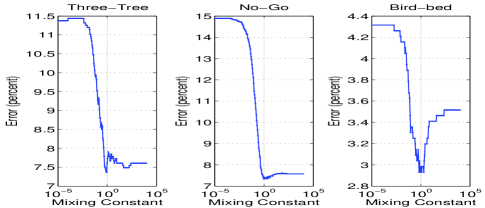
Figure 5: Classifier combination results for each class pair as a function of linear combination weight. Performance at the far right of each graph corresponds to CNN only and far left to PBN.

III-G Random Synthesis

As a final demonstration of generative power, we synthesized entirely random events by starting with random data equal in dimension to the PBN output layer, in this case dimension-2. Data was synthesized at the point prior to the output activation function using Gaussian random variables. Results are shown in Figure 6 for the class pair “three” and “tree”.

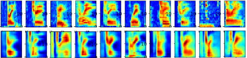
Figure 6: Top: ten training samples randomly selected from “three” and “tree” spoken word commands. Bottom: randomly synthesized data from trained PBN. There is no relationship to the selected training samples on top.

The synthetic samples appear realistic and are diverse, showing variations in time shift, dilation, and other qualities. This means that the PBN has indeed learned much about the data generation process.

III-H Implementation and Applications

The PBN was implemented in Python using Theano symbolic expression compiler [22]. The primary computational challenge is the solution of a symmetric linear system with dimension $M\times M$, where $M$ is the total output dimension of a layer. This must be solved for each iteration in the solution of (2). This was parallelized on the GPU, one processor for sample in a mini-batch. The computational time for an epoch was 1.1 seconds. This was only about an order of magnitude slower than training the DNN. All results were obtained using PBN Toolkit .

IV Conclusions

In this paper, a projected belief network (PBN), which is a purely generative layered network, was trained as a generative-discriminative classifier. This was achieved using a label-dependent prior for the output features. Since the PBN is based on a feed-forward neural network (FF-NN), it can share an embodiment with a discriminative deep neural network (DNN). Through the parameter $C$, the network can be trained with varying amount of discriminative influence. When reconstructing visible data from the hidden variables, it was shown that the the same netrork, trained discriminatively, had very poor ability to reconstruct, even from initial layers, whereas whe the network was trained as a PBN, the reconstruction greatly improved. The PBN classifier had comparable classification performance to the discriminatively-trained network, yet provided generative power from three standpoints: visible data reconstruction from hidden variables, random data synthesis, and classification of out-of set samples. It was also shown to improve upon a conventional CNN when additively combined.

References

- [1] J. Lasserre, C. Bishop, and T. Minka, “Principled hybrids of generative and discriminative models,” vol. 1, pp. 87– 94, 07 2006.
- [2] C. Mayer and R. Timofte, “Adversarial sampling for active learning,” arXiv:1808.06671, to appear WACV 2020, 2019.
- [3] T. Jaakkola and D. Haussler, “Exploiting generative models in discriminative classifiers,” tech. rep., Dept. of Computer Science, Univ. of California, 1998.
- [4] R. Raina, Y. Shen, A. Ng, and A. McCallum, “Classification with hybrid generative /discriminative models,” in Proceedings of NIPS (Neural Information Processing Systems) 2004, 2004.
- [5] S. Fine, J. Navratil, and R. Gopinath, “Enhancing gmm scores using SVM hints,” in Proceedings of the 7th European Conference on Speech Communication and Technology (EuroSpeech), 2001.
- [6] A. Fujino, N. Ueda, and K. Saito, “A hybrid generative/discriminative approach to semi-supervised classifier design,” in Proceedings of the National Conference on Artificial Intelligence, vol. 20, 2005.
- [7] A. Holub, M. Welling, and P. Perona, “Hybrid generative-discriminative visual categorization,” in Proceedings of the International Journal of Computer Vision, vol. 77, pp. 239–258, 2008.
- [8] A. Bosch, A. Zisserman, and X. Muoz, “Scene classification using a hybrid generative/discriminative approach,” IEEE Transactions on Pattern Analysis and Machine Intelligence, vol. 30, no. 4, pp. 712–727, 2008.
- [9] T. Minka, “Discriminative models, not discriminative training,” Microsoft Research Ltd, technical report, 2005.
- [10] C. Bishop and J. Lasserre, “Generative or discriminative? getting the best of both worlds,” Bayesian Statistics, vol. 8, pp. 3–24, 2007.
- [11] V. Vapnik, The Nature of Statistical Learning. Springer, 1999.
- [12] M. Welling, M. Rosen-Zvi, and G. Hinton, “Exponential family harmoniums with an application to information retrieval,” Advances in neural information processing systems, 2004.
- [13] G. E. Hinton, S. Osindero, and Y.-W. Teh, “A fast learning algorithm for deep belief nets,” in Neural Computation 2006, 2006.
- [14] D. J. Rezende, S. Mohamed, and D. Wierstra, “Stochastic backpropagation and approximate inference in deep generative models,” in Proceedings of the 31st International Conference on Machine Learning (E. P. Xing and T. Jebara, eds.), vol. 32 of Proceedings of Machine Learning Research, (Bejing, China), pp. 1278–1286, PMLR, 22–24 Jun 2014.
- [15] I. Goodfellow, J. Pouget-Abadie, M. Mirza, B. Xu, D. Warde-Farley, S. Ozair, A. Courville, and Y. Bengio, “Generative adversarial nets,” in Advances in Neural Information Processing Systems 27 (Z. Ghahramani, M. Welling, C. Cortes, N. D. Lawrence, and K. Q. Weinberger, eds.), pp. 2672–2680, Curran Associates, Inc., 2014.
- [16] P. M. Baggenstoss, “On the duality between belief networks and feed-forward neural networks,” IEEE Transactions on Neural Networks and Learning Systems, pp. 1–11, 2018.
- [17] P. M. Baggenstoss, “Applications of projected belief networks (pbn),” in Proceedings of EUSIPCO 2019, (La Coruña, Spain), Sep 2019.
- [18] P. M. Baggenstoss, “Maximum entropy PDF design using feature density constraints: Applications in signal processing,” IEEE Trans. Signal Processing, vol. 63, June 2015.
- [19] P. M. Baggenstoss, “A neural network based on first principles,” in arXiv:2002.07469, submitted to ICASSP 2020, (Barcelona, Spain), Sep 2020.
- [20] P. M. Baggenstoss, “Uniform manifold sampling (UMS): Sampling the maximum entropy pdf,” IEEE Transactions on Signal Processing, vol. 65, pp. 2455–2470, May 2017.
- [21] P. Warden, “Speech commands: A dataset for limited-vocabulary speech recognition,” arXiv:1804.03209, 2018.
- [22] J. Bergstra, O. Breuleux, F. Bastien, P. Lamblin, R. Pascanu, G. Desjardins, J. Turian, D. Warde-Farley, and Y. Bengio, “Theano: A cpu and gpu math expression compiler,” Proceedings of the Python for Scientific Computing Conference (SciPy) 2010, 2010.