$DK$ $I=0,$ $D\bar{K}$ $I=0,1$ scattering and the $D_{s0}^{\ast}(2317)$ from lattice QCD

Abstract

Elastic scattering amplitudes for $I=0$ $DK$ and $I=0,1$ $D\bar{K}$ are computed in $S$, $P$ and $D$ partial waves using lattice QCD with light-quark masses corresponding to $m_{\pi}=239$ MeV and $m_{\pi}=391$ MeV. The $S$-waves contain interesting features including a near-threshold $J^{P}=0^{+}$ bound state in $I=0$ $DK$, corresponding to the $D_{s0}^{\ast}(2317)$, with an effect that is clearly visible above threshold, and suggestions of a $0^{+}$ virtual bound state in $I=0$ $D\bar{K}$. The $S$-wave $I=1$ $D\bar{K}$ amplitude is found to be weakly repulsive. The computed finite-volume spectra also contain a deeply-bound $D^{\ast}$ vector resonance, but negligibly small $P$-wave $DK$ interactions are observed in the energy region considered; the $P$ and $D$-wave $D\bar{K}$ amplitudes are also small. There is some evidence of $1^{+}$ and $2^{+}$ resonances in $I=0$ $DK$ at higher energies.

1 Introduction

Many questions in hadron spectroscopy remain unanswered following recent precision data from experiments investigating the charm quark. These studies revealed a number of surprising features. While the best known are the so-called “$XYZ$s”, some of which appear as charmonium-like states close to thresholds for two-meson decay, open-charm mesons also show unexpected properties. Ultimately, forming a complete understanding of mesons requires calculation of the scattering amplitudes involving meson states. Since the dynamics of hadrons is governed by quantum chromodynamics (QCD) which is strongly coupled at hadronic energy scales, a non-perturbative method is needed. A lattice regularisation of the QCD path integral provides just such a technique, amenable to large-scale numerical investigation. The aim of lattice spectroscopy studies is to connect experimentally-observed hadron resonances directly with the QCD Lagrangian in order to learn more about the confined constituents of these states. With a more complete understanding of scattering involving mesons made of charm quarks as a goal, the work described in this paper investigates the charm-anti-strange and charm-strange sectors.

The $D_{s0}^{\ast}(2317)$ charm-anti-strange scalar meson, first observed by the BaBar collaboration Aubert:2003fg , has attracted significant attention. The mass is much lower than predicted by the quark model Godfrey:1985xj , where it is described as a spin-triplet $P$-wave orbital excitation, and is surprisingly close to the corresponding charm-light scalar state, $D_{0}^{\ast}(2400)$. The $D_{s0}^{\ast}(2317)$ appears as a very narrow resonance below the $DK$ threshold and decays almost entirely to $D_{s}^{+}\pi^{0}$, breaking isospin symmetry. This contrasts strongly with the $D_{0}^{\ast}(2400)$, found above the corresponding $D\pi$ threshold and seen as a broad resonance close to predictions from the quark model. A number of explanations for the failure of the quark model to predict the $D_{s0}^{\ast}(2317)$ meson mass reliably have been postulated, the most common modelling it as a $DK$ molecule, a tetraquark or a conventional meson which has its properties modified by coupling to $DK$ (see for example Ref. Chen:2016spr for a recent review). An axial-vector state, $D_{s1}(2460)$, was also discovered Besson:2003jp and similarly does not fit easily into expectations based on a quark model. While this article was being finalised, LHCb announced the observation of a structure in the exotic-flavour $D^{-}K^{+}$ ($\bar{c}\bar{s}du$) channel at an energy $\sim 2.9$ GeV LHCbCharmStrange:2020 ; Aaij:2020hon ; Aaij:2020ypa .

We have recently performed a lattice QCD calculation of the coupled-channel $D\pi$, $D\eta$, $D_{s}\bar{K}$ isospin-1/2 scattering amplitudes Moir:2016srx in an attempt to understand the $D_{0}^{\ast}(2400)$. The scattering amplitudes were analytically continued in the complex plane and a scalar bound state was found just below the $D\pi$ threshold. This calculation was performed with unphysically-heavy light quarks corresponding to $m_{\pi}=391$ MeV and calculations closer to the physical point are required to make a more definite comparison with the experimentally-observed state.

This work focuses on the charm-anti-strange and charm-strange sectors, calculating the isoscalar ($I=0$) $DK$ elastic scattering amplitudes in $S$, $P$ and $D$ partial waves, along with isoscalar and isovector ($I=0$ and $1$) $D\bar{K}$ scattering. Computations are performed on two sets of Monte Carlo ensembles of gauge configurations, sampled with light-quark masses corresponding to pion masses of approximately $239$ and $391$ MeV. A large range of finite-volume spectra is extracted for various irreducible representations of the group of spatial rotations, including for systems with overall non-zero momentum with respect to the lattice. From the energy levels, the infinite-volume scattering amplitudes are constrained using the Lüscher method and then analytically continued in the complex plane where the pole singularities correspond to bound states and resonances. A scalar bound state is found in $I=0$ $DK$ which we identify with the $D_{s0}^{\ast}(2317)$. In addition, a deeply bound state and a resonance are found in the $P$ and $D$ wave scattering amplitudes respectively. For both the $S$ and $P$-wave bound states, comparisons between the two sets of ensembles show little light-quark mass dependence. In addition, we find suggestions of a virtual bound state in $S$-wave $D\bar{K}$. Some preliminary results from these calculations have appeared in Refs. Thomas:2016euu ; Cheung:2019fsx .

The rest of this paper is organised as follows: Sections 2 and 3 give the calculation details and lattice parameters. Results for the finite-volume spectra are presented in Section 4 and the scattering amplitudes, derived using Lüscher’s framework, are given in Section 5. In Section 6 we analytically continue the amplitudes to the complex energy plane and find the location of pole singularities, interpret the results and compare with previous lattice calculations which have studied $DK$/$D\bar{K}$ scattering Liu:2012zya ; Mohler:2013rwa ; Lang:2014yfa ; Bali:2017pdv ; Alexandrou:2019tmk . A summary and outlook are presented in Section 7.

2 Calculation details

Lattice QCD calculations are performed in a finite volume leading to the quantisation of momentum and a discrete spectrum. For a cubic spatial volume with periodic boundary conditions such as that used in this work, momentum is quantised as $\vec{P}=\frac{2\pi}{L}(n_{x},n_{y},n_{z})$, where $L$ is the spatial extent and $n_{i}$ are integers; we will use a shorthand notation $[n_{x}n_{y}n_{z}]$. Furthermore, the finite volume and lattice discretisation break the continuous rotational symmetry of an infinite-volume continuum. This means that angular momentum, $J$, is not a good quantum number and states must instead be labelled by the irreducible representations (irreps) of the remaining symmetry group. For a cubic lattice and spatial volume, the relevant group is the octahedral group with parity, $O_{h}$, for mesons at rest Johnson:1982yq and the smaller little group, $\text{LG}(\vec{P})$, for mesons at non-zero momentum $\vec{P}$ Moore:2005dw .

We will follow our well-established procedure to determine the finite-volume spectrum in each channel. A matrix of correlation functions is computed,

$$C_{ij}(t)=\langle 0|\mathcal{O}_{i}^{\vphantom{\dagger}}(t)\mathcal{O}_{j}^{\dagger}(0)|0\rangle\,$$ (1)

for a basis of interpolating operators, $\{\mathcal{O}_{i}\}$, with the appropriate quantum numbers. The spectrum is then extracted using a variational method where a generalised eigenvalue problem $C_{ij}(t)v^{\mathfrak{n}}_{j}=\lambda^{\mathfrak{n}}(t,t_{0})C_{ij}(t_{0})v^{\mathfrak{n}}_{j}$ is solved for some appropriate choice of $t_{0}$ Michael:1985ne ; Luscher:1990ck . The $\mathfrak{n}$’th eigenvalue $\lambda^{\mathfrak{n}}$, referred to as a principal correlator, is related to the energy $E_{\mathfrak{n}}$ of the $\mathfrak{n}$’th energy eigenstate $|\mathfrak{n}\rangle$. In our implementation, detailed in Refs. Dudek:2007wv ; Dudek:2010wm , the energies are obtained by fitting the principal correlators to the form $\lambda^{\mathfrak{n}}(t,t_{0})=(1-A_{\mathfrak{n}})e^{-E_{\mathfrak{n}}(t-t_{0})}+A_{\mathfrak{n}}e^{-E^{\prime}_{\mathfrak{n}}(t-t_{0})}$; the fit parameters are $E_{\mathfrak{n}},E_{\mathfrak{n}}^{\prime}$ and $A_{\mathfrak{n}}$, and the second exponential is used to account for possible contamination from excited states. The eigenvectors, $v^{\mathfrak{n}}_{j}$, are related to the matrix elements, $Z_{i}^{\mathfrak{n}}=\langle\mathfrak{n}|\mathcal{O}_{i}^{\dagger}|0\rangle$, and can be used to construct the variationally-optimal combination of $\{\mathcal{O}_{i}\}$ to interpolate $|\mathfrak{n}\rangle$, $\Omega_{\mathfrak{n}}^{\dagger}=\sum_{i}v^{\mathfrak{n}}_{i}\mathcal{O}^{\dagger}_{i}$.

The basis of operators used must have an appropriate variety of structures to robustly extract the finite-volume states of interest (see e.g. Refs. Dudek:2012xn ; Wilson:2015dqa ; Cheung:2017tnt ). In this work, we use single-meson operators, $\mathcal{O}^{\Lambda\mu}_{\mathbb{M}}(\vec{P})$, with a structure resembling a single meson, and meson-meson operators, $\mathcal{O}^{\Lambda\mu}_{\mathbb{M}_{1}\mathbb{M}_{2}}(\vec{P})$, with a structure resembling two mesons, projected onto definite momentum, $\vec{P}$, and transforming in an irrep, $\Lambda$, and row, $\mu$, of the relevant symmetry group. Single-meson operators Dudek:2010wm ; Thomas:2011rh are constructed from fermion bilinears, $\sum_{\vec{x}}e^{i\vec{P}\cdot\vec{x}}\bar{\psi}\Gamma\overleftrightarrow{D}\dots\psi$, with a definite $J$ that are then subduced to the lattice irrep. Meson-meson operators Dudek:2012gj ; Dudek:2012xn are constructed from the product of two single-meson operators, $\sum_{\vec{p}_{1},\vec{p}_{2}}\mathcal{C}(\vec{p}_{1},\vec{p}_{2})\Omega_{\mathbb{M}_{1}}^{\dagger}(\vec{p}_{1})\Omega^{\dagger}_{\mathbb{M}_{2}}(\vec{p}_{2})$ where $\mathcal{C}$ is a generalised Clebsch-Gordan coefficient and and $\Omega_{\mathbb{M}_{i}}^{\dagger}(\vec{p}_{i})$ is a variationally-optimised operator for interpolating meson $\mathbb{M}_{i}$. Previous calculations have suggested that local tetraquark-like operators have little effect on the spectra Cheung:2017tnt ; Padmanath:2015era . Because we only consider an energy region well below any relevant three-meson thresholds, we do not include operators constructed with a structure resembling three or more mesons Cheung:2017tnt ; Woss:2019hse . The specific bases of operators we use for each channel are presented in Appendix A.

To calculate the matrix of two-point correlation functions, we use the distillation framework Peardon:2009gh . In this approach, the quark fields appearing in interpolating operators are smeared with a distillation operator, $\Box(t)=\sum^{N_{\text{vecs}}}_{i=1}\xi_{i}(t)\xi_{i}^{\dagger}(t)$, where $\xi_{i}$ are the lowest $N_{\text{vecs}}$ eigenvectors of the discretised gauge-covariant Laplacian. This procedure factorises the computation of correlation functions and allows us to consider operators with various structures where each operator is projected onto a definite momentum. In addition, distillation enables contributions to Wick contractions where quark fields annihilate to be computed efficiently. A schematic representation of the diagrams contributing to isospin-0 $DK$ and isospin-0 and 1 $D\bar{K}$ is presented in Fig. 1.

Figure 1: A schematic representation of the types of Wick contraction topologies that contribute to isospin-0 $DK$ and isospin-0 and 1 $D\bar{K}$ correlation functions involving $D_{s}$ (single-meson) and $DK/\bar{K}$ (meson-meson) operators. The grey ellipses represent fermion-bilinear operators with various structures or sums of such operators. For each irrep we compute sums of several thousand Wick contractions with these sorts of topologies.

3 Lattice details

Ensemble	$(L/a_{s})^{3}\times(T/a_{t})$	$N_{\text{cfgs}}$	$N_{\text{tsrcs}}$	$N_{\text{vecs}}$
$m_{\pi}=239$ MeV	$32^{3}\times 256$	484	1 ($DK$, $D\bar{K}$, disp)	256
$m_{\pi}=391$ MeV	$16^{3}\times 128$	478	8 ($DK$, $D\bar{K}$, disp)	64
	$20^{3}\times 128$	603	3 ($DK$, $D\bar{K}$), 4 (disp)	128
	$24^{3}\times 128$	553	1 ($DK$), 1-3 ($D\bar{K}$), 4 (disp)	162

Table 1: Summary of the lattice ensembles used in this work. The volume is given by $(L/a_{s})^{3}\times(T/a_{t})$ where $L$ and $T$ are the spatial and temporal extents of the lattice. $N_{\text{cfgs}}$ is the number of gauge field configurations used, $N_{\text{tsrcs}}$ is the number of time-sources used per configuration, and $N_{\text{vecs}}$ is the number of distillation vectors in the distillation framework. The number of time sources used to compute the momentum dependence of the $D_{(s)}^{(\ast)}$ energies for the dispersion relation fits, Fig. 2, are indicated by “disp”.

We perform calculations on anisotropic lattices where the temporal lattice spacing, $a_{t}$, is smaller than the spatial lattice spacing, $a_{s}\approx 0.12$ fm, such that $\xi=a_{s}/a_{t}\approx 3.5$ – the finer resolution in time enables a better extraction of finite-volume energies from two-point correlation functions. The discretised QCD action consists of a tree-level Symanzik-improved gauge action and a Wilson-clover fermion action with $N_{f}=2+1$ flavours of dynamical quarks (two degenerate light up and down quarks and a heavier strange quark) Edwards:2008ja ; Lin:2008pr . In this work we use two sets of ensembles: one volume where the light quark mass parameter is tuned such that $m_{\pi}=239$ MeV and three volumes with $m_{\pi}=391$ MeV; in both cases the strange quark is tuned to approximate the physical strange quark mass. The quenched charm quark is described by the same action with the mass parameter tuned to reproduce the physical $\eta_{c}$ meson mass Liu:2012ze ; Cheung:2016bym . Details of the lattice ensembles used are summarised in Table 1.

When quoting results in physical units, we set the scale using the mass of the $\Omega$ baryon to determine $a_{t}^{-1}=m_{\Omega}^{\textrm{phys}}/a_{t}m_{\Omega}$. This gives $a_{t}^{-1}=6079$ MeV for the $m_{\pi}=239$ MeV ensemble Wilson:2019wfr and $a_{t}^{-1}=5667$ MeV for $m_{\pi}=391$ MeV Edwards:2011jj .

	$a_{t}m$
$m_{\pi}$	239 MeV	391 MeV
$\pi$	0.03928(18) Wilson:2015dqa	0.06906(13) Dudek:2012gj
$K$	0.08344(7)  Wilson:2015dqa	0.09698(9) Wilson:2014cna
$\eta$	0.09299(56) Wilson:2015dqa	0.10364(19) Dudek:2016cru
$D$	0.30923(11) Cheung:2016bym	0.33303(31)
$D_{s}$	0.32356(12)	0.34441(29)
$D^{\ast}$	0.33058(24)	0.35494(46)
$D_{s}^{\ast}$	0.34448(15)	0.36587(35)

	$a_{t}E_{\mathrm{threshold}}$
$m_{\pi}$	$239$ MeV	$391$ MeV
$DK$	0.39267(13)	0.4300(3)
$D_{s}\eta$	0.4166(6)	0.4481(3)
$D^{\ast}K$	0.4140(3)	0.4519(5)
$D_{s}^{\ast}\eta$	0.4375(6)	0.4695(4)
$D_{s}\pi\pi$	0.4021(3)	0.4825(3)
$D_{s}^{\ast}\pi\pi$	0.4230(3)	0.5040(4)

Table 2: Left: relevant stable meson masses for the $m_{\pi}=239$ MeV and $m_{\pi}=391$ MeV ensembles from dispersion fits. Right: relevant kinematic thresholds.

The masses of stable mesons used when extracting scattering amplitudes, along with masses of other relevant stable mesons and kinematic thresholds, are summarised in Table 2. The anisotropy, $\xi$, can be determined by fitting the momentum dependence of a stable hadron’s energy to the relativistic dispersion relation Dudek:2012gj . On the $m_{\pi}=239$ MeV ensemble, $\xi_{\pi}=3.453(6)$, $\xi_{K}=3.462(4)$ Wilson:2015dqa and $\xi_{D}=3.443(7)$ Cheung:2016bym from the $\pi$, $K$ and $D$ meson respectively, which are broadly consistent within statistical uncertainties. In the calculations of scattering amplitudes we will take $\xi=\xi_{\pi}=3.453(6)$, but when estimating contributions to the systematic uncertainties we use values spanning the range of these anisotropies, $\xi=3.436$ and $3.466$. For the $D$ meson mass on this ensemble we use the result of the fit to the dispersion relation in Ref. Cheung:2016bym and analogous fits for the $D_{s}$ and $D_{(s)}^{\ast}$ mesons.

On the $m_{\pi}=391$ MeV ensembles, $\xi_{\pi}=3.444(6)$ Dudek:2012gj and $\xi_{K}=3.449(4)$ Wilson:2014cna . For the $D$ meson we update the original dispersion fit presented in Ref. Liu:2012ze with a fit that includes all the propagators now available and the $20^{3}$ volume – Fig. 2 summarises the results. The right panel shows a fit on the largest volume which gives $\xi_{D}=3.466(4)$. We will use $\xi=\xi_{\pi}=3.444(6)$, but when estimating some of the systematic uncertainties we use values spanning the range of the $\pi$, $K$ and $D$ anisotropies, $\xi=3.438$ and $3.470$. As the central values for the charm meson masses (see Table 2) we take the average from fits to the dispersion relations on the $20^{3}$ and $24^{3}$ volumes separately, and for the uncertainty we quote a value which spans the central values and uncertainties obtained from those fits.

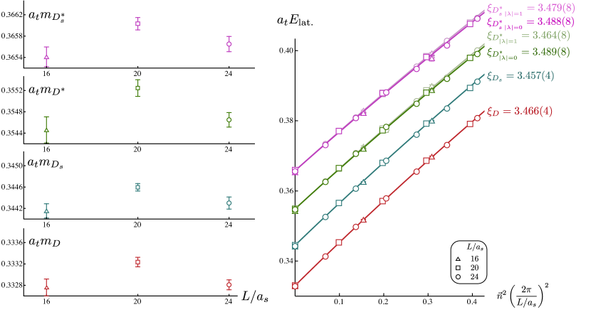
Figure 2: Charmed meson masses and dispersion relation fits on the ensembles with $m_{\pi}~{}=~{}391$ MeV. Left panel shows meson masses extracted on each volume from a fit to the dispersion relation on that volume. Right panel shows the meson energies from all three volumes as a function of momentum and results of fits to the dispersion relation on the largest volume – these all give a reasonable fit to the data.

In the left panel of Fig. 2 it can be seen that on each volume the mass of the $D$ meson is extracted with high statistical precision and there are small but statistically significant differences between the different volumes. To allow for this systematic effect in our analyses, we add an additional systematic uncertainty to each finite-volume energy level on the $m_{\pi}=391$ MeV ensembles via,

$$a_{t}\delta E_{\mathrm{lat.}}\to a_{t}\delta E_{\mathrm{lat.+syst.}}=a_{t}\left(\delta E_{\mathrm{lat.}}^{2}+\delta E_{\mathrm{syst.}}^{2}\right)^{\frac{1}{2}}\,,$$

where we estimate $\delta E_{\mathrm{syst.}}=0.00021$ to span an envelope of the central values of the $D$ meson masses on the $20^{3}$ and $24^{3}$ volumes.

4 Finite-volume spectra

In this section we first present the finite-volume spectra obtained in the isospin-0 $DK$ sector on the $m_{\pi}=239$ MeV and $m_{\pi}=391$ MeV ensembles, and then show the analogous isospin-0 and isospin-1 $D\bar{K}$ results. The $J^{P}$ and pseudoscalar-pseudoscalar partial waves, $\ell$, which contribute to the different irreps are presented in Table 3. These spectra are analysed to determine scattering amplitudes in Section 5.

$\vec{P}$	LG$(\vec{P})$	$\Lambda$	$\,\,J^{P}(\vec{P}=\vec{0})$	$\ell^{N}$
			$\left|\lambda\right|^{({\tilde{\eta}})}(\vec{P}\neq\vec{0})$
$\left[0,0,0\right]$	$\textrm{O}_{h}^{\textrm{D}}$ ($\textrm{O}_{h}$)	$A_{1}^{+}$	$0^{+},\,4^{+}$	$0^{1},\,4^{1}$
		$T_{1}^{-}$	$1^{-},\,3^{-},\,\mathit{(4^{-})}$	$1^{1},\,3^{1}$
		$E^{+}$	$2^{+},\,4^{+}$	$2^{1},\,4^{1}$
		$T_{2}^{+}$	$2^{+},\,4^{+},\,\mathit{(3^{+})}\,$	$2^{1},\,4^{1}$
		$T_{1}^{+}$	$4^{+},\,\mathit{(1^{+},3^{+})}$	$4^{1}$
		$T_{2}^{-}$	$3^{-},\,\mathit{(2^{-},4^{-})}$	$3^{1}$
		$A_{2}^{-}$	$3^{-}$	$3^{1}$
$\left[0,0,n\right]$	Dic4 ($\textrm{C}_{4\textrm{v}}$)	$A_{1}$	$0^{+},\,4$	$0^{1},\,1^{1},\,2^{1},\,3^{1},\,4^{2}$
		$E_{2}$	$1,\,3$	$1^{1},\,2^{1},\,3^{2},\,4^{2}$
		$B_{1}$	$2$	$2^{1},\,3^{1},\,4^{1}$
		$B_{2}$	$2$	$2^{1},\,3^{1},\,4^{1}$
		$A_{2}$	$4,\,\mathit{(0^{-})}$	$4^{1}$
$\left[0,n,n\right]$	Dic2 ($\textrm{C}_{2\textrm{v}}$)	$A_{1}$	$0^{+},\,2,\,4$	$0^{1},\,1^{1},\,2^{2},\,3^{2},\,4^{3}$
		$B_{1}$	$1,\,3$	$1^{1},\,2^{1},\,3^{2},\,4^{2}$
		$B_{2}$	$1,\,3$	$1^{1},\,2^{1},\,3^{2},\,4^{2}$
		$A_{2}$	$2,\,4,\,\mathit{(0^{-})}$	$2^{1},\,3^{1},\,4^{2}$
$\left[n,n,n\right]$	Dic3 ($\textrm{C}_{3\textrm{v}}$)	$A_{1}$	$0^{+},\,3$	$0^{1},\,1^{1},\,2^{1},\,3^{2},\,4^{2}$
		$E_{2}$	$1,\,2,\,4$	$1^{1},\,2^{2},\,3^{2},\,4^{3}$
		$A_{2}$	$3,\,\mathit{(0^{-})}$	$3^{1},\,4^{1}$

Table 3: The pattern of subductions of pseudoscalar-pseudoscalar partial waves, $\ell\leq 4$, into lattice irreps, $\Lambda$, when the pseudoscalars have unequal mass, e.g. $DK$ or $D\bar{K}$ (from Table III of Ref. Wilson:2014cna ). Here $N$ is the number of embeddings of this $\ell$ in the irrep and $n$ is a non-zero integer. LG$(\vec{P})$ is the double-cover little group and the corresponding single-cover little group relevant for only integer spin is given in parentheses. Also shown are the various $J\leq 4$ or $|\lambda|\leq 4$ that appear in each of the relevant irreps. The $J^{P}$ values and $|\lambda|^{\tilde{\eta}}=0^{-}$ in italics are in the “unnatural parity” [$P=(-1)^{J+1}$] series and do not contribute to pseudoscalar-pseudoscalar scattering.

4.1 $DK$ $I=0$ with $m_{\pi}=239$ MeV

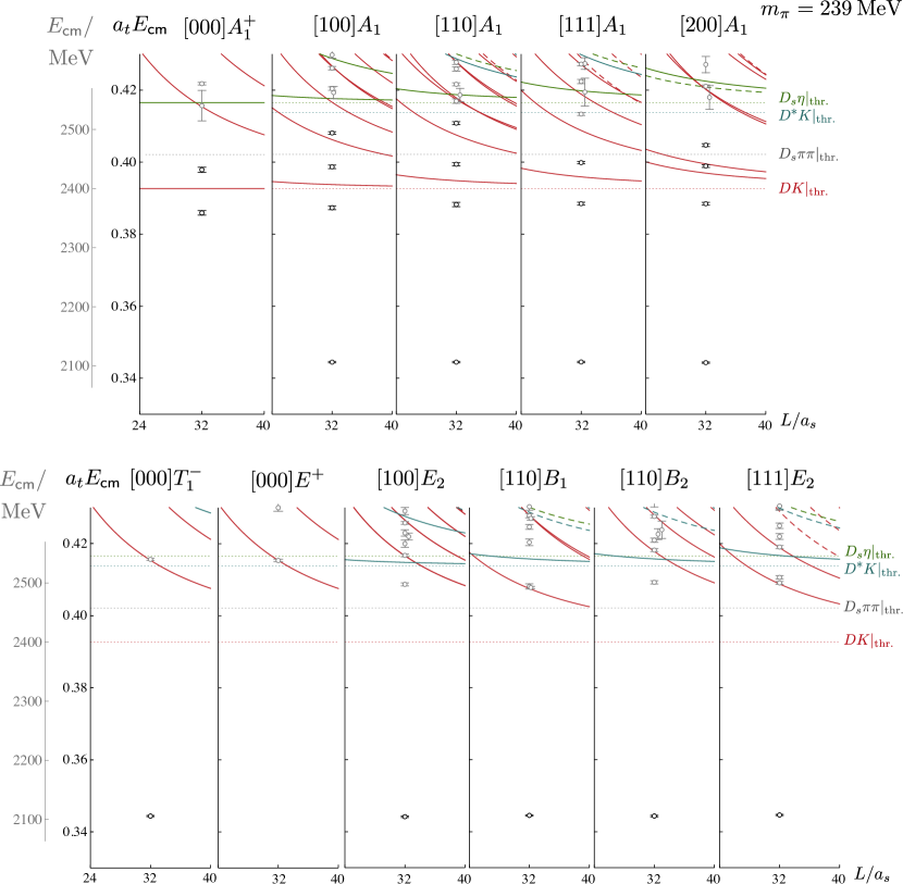
Figure 3: $DK$ $I=0$ finite-volume spectra on the $m_{\pi}=239$ MeV ensemble labelled by $[\vec{P}]\Lambda^{(P)}$. Points show the extracted finite-volume energy levels transformed to the centre-of-momentum frame; black points are used in the scattering analysis whilst grey points are not. Dotted lines show relevant kinematic thresholds. Solid lines/curves show non-interacting energies with dashed curves indicating non-interacting energies where the corresponding operator was not included in the basis.

The extracted $DK$ $I=0$ finite-volume spectra on the $m_{\pi}=239$ MeV ensemble, computed using the operators listed in Table 6 in Appendix A, are shown in Fig. 3 labelled by $[\vec{P}]\Lambda^{(P)}$, where parity, $P$, is a good quantum number for $\vec{P}=\vec{0}$. Along with the computed energies, kinematic thresholds and non-interacting energies are also shown. In the scattering analyses we use the energy levels below $D^{\ast}K$ threshold in the $A_{1}^{+}$ and $A_{1}$ irreps, and levels below $D_{s}\pi\pi$ threshold in other irreps – these are shown as black points in the figure. Some representative examples of the underlying principal correlator fits are given in Appendix B.

We will analyse these spectra to determine scattering amplitudes in Section 5, but here we make some qualitative observations. The top row of Fig. 3 shows irreps where the lowest contributing partial wave is $\ell=0$. The presence of an ‘extra’ energy level in the energy region $a_{t}E_{\text{cm}}\approx 0.38-0.41$ compared to the number expected in the absence of meson-meson interactions, as well as shifts away from the non-interacting energy levels, suggests there are significant $DK$ interactions. This feature could arise from a $J^{P}=0^{+}$ bound state or resonance in $S$-wave $DK$ scattering.

An additional ‘extra’ energy level is seen at $a_{t}E_{\text{cm}}\approx 0.34$ far below $DK$ threshold in $A_{1}$ irreps with $\vec{P}\neq\vec{0}$ – these contain $\ell=1$ contributions, suggesting a deeply bound $1^{-}$ state in $P$-wave. Further evidence for this can be seen in the irreps in the bottom row of Fig. 3 which have $\ell=1$ as the lowest contributing partial wave (all except for $[000]E^{+}$ where $\ell=2$ is the lowest partial wave), where a similar energy level is found.

It is interesting to note the presence of another ‘extra’ level below $D^{\ast}K$ threshold in the $[100]E_{2}$, $[110]B_{1,2}$ and $[111]E_{2}$ irreps at $a_{t}E_{\text{cm}}\approx 0.41$. Such an energy level could arise from a bound state or resonance in $D^{\ast}K$ scattering with $J^{P}=1^{+}$. We only consider elastic $DK$ scattering in this study and an extended coupled-channel analysis would be needed to draw further conclusions on this – we return to this point in Section 5.1.3.

The $[000]E^{+}$ irrep shown in the bottom row of Fig. 3 has $\ell=2$ as the lowest contributing partial wave. The lowest level shows no significant shift away from the associated non-interacting energy, suggesting no significant interactions in this energy region. However, at higher energies we observe ‘extra’ levels which have dominant overlap with $c\bar{s}$ fermion-bilinear constructions subduced from $J^{P}=2^{+}$ continuum operators.

4.2 $DK$ $I=0$ with $m_{\pi}=391$ MeV

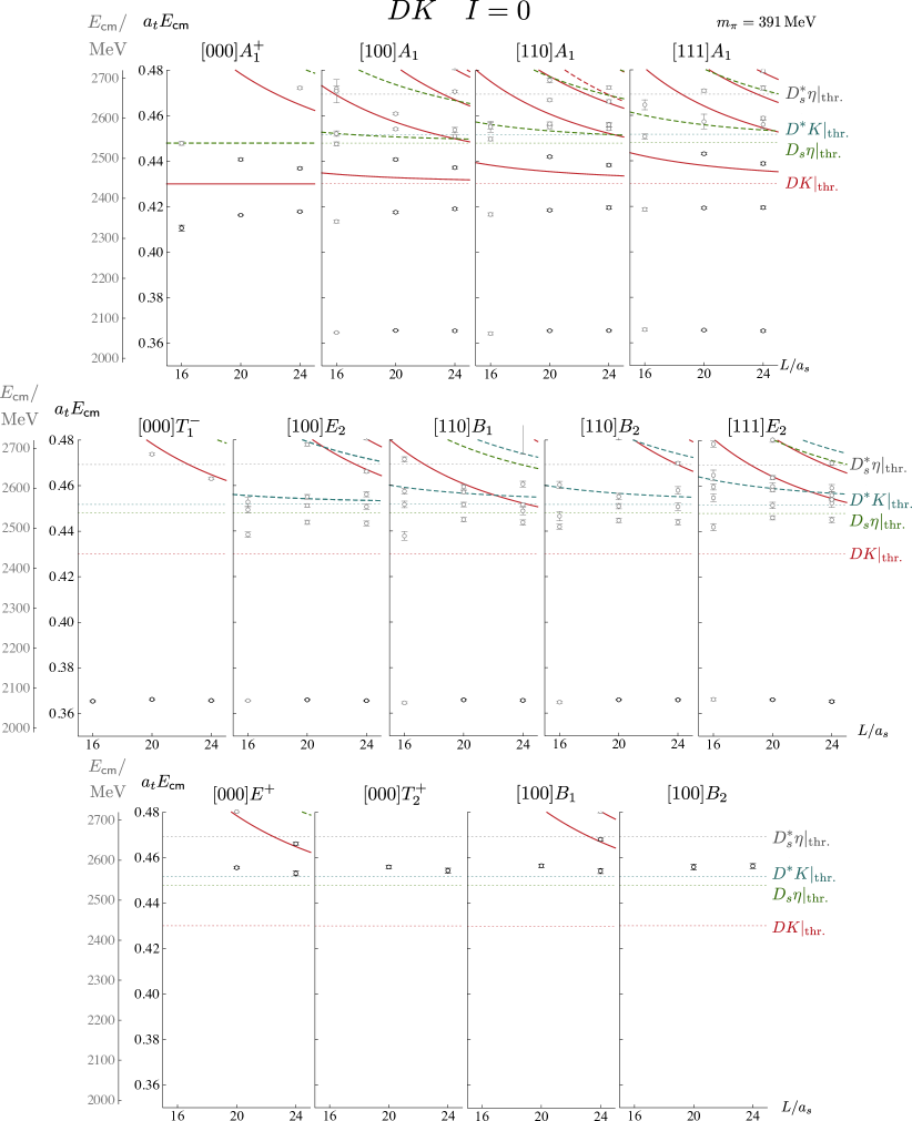
Figure 4: As Figure 3 but for $I=0$ $DK$ on the $m_{\pi}=391$ MeV ensembles.

Finite-volume spectra for $DK$ $I=0$ with $m_{\pi}=391$ MeV are presented in Fig. 4, computed using the operators listed in Table 7. The energy levels we use in the scattering analyses are shown as black points – these are the levels well below $D_{s}\eta$ threshold in the irreps where the lowest contribution is $\ell=0$ or $1$ $DK$, and the low-lying levels in other irreps; on the $16^{3}$ volume we only use the $[000]A_{1}^{+}$ and $[000]T_{1}^{+}$ irreps. Some representative examples of the underlying principal correlator fits are again given in Appendix B.

The spectra show similar qualitative features to the $m_{\pi}=239$ MeV spectra in Fig. 3. An ‘extra’ level is observed in the energy region $a_{t}E_{\text{cm}}\approx 0.41-0.45$ in irreps which have contributions from $\ell=0$. A level is found around $a_{t}E_{\text{cm}}\approx 0.36$ far below $DK$ threshold in irreps which contain contributions from $\ell=1$, suggesting a $1^{-}$ deeply bound state.

The bottom row of Fig. 4 shows irreps which have $\ell=2$ as the lowest contributing partial wave. The presence of an ‘extra’ energy level in the energy region $a_{t}E_{\text{cm}}\approx 0.45-0.46$ and shifts of levels away from non-interacting energies suggests that there is a non-trivial interaction in $D$-wave $DK$.

4.3 $D\bar{K}$ $I=0,1$ with $m_{\pi}=239$ MeV

Finite-volume spectra for $D\bar{K}$ with $I=0$ and $I=1$ on the $m_{\pi}=239$ MeV ensemble, computed using the operators listed in Table 8, are shown in Fig. 5. These exotic-flavour combinations cannot be interpolated by single-meson (fermion-bilinear) operators, quark-line annihilations are not possible and, as shown in Fig. 1, each Wick diagram contains exactly four quark lines that propagate from source to sink. In the scattering analyses we use the energy levels shown in black in Fig. 5 – these levels are well below $D\bar{K}\pi$ threshold and the lowest non-interacting $D^{\ast}\bar{K}$ energy level. Some representative examples of the underlying principal correlator fits are given in Appendix B.

The qualitative pattern of energy levels is very different to the case of $I=0$ $DK$. For both isospins, we see no sign of any ‘extra’ levels and the energies show only small shifts away from the non-interacting energies, suggesting weak interactions. However, in the $I=0$ channel there are negative shifts in irreps where $\ell=0$ contributes, suggesting an attractive $S$-wave interaction, with very small shifts in other irreps. In the $I=1$ channel there are small positive shifts in the irreps with $\ell=0$ suggesting weak repulsion.

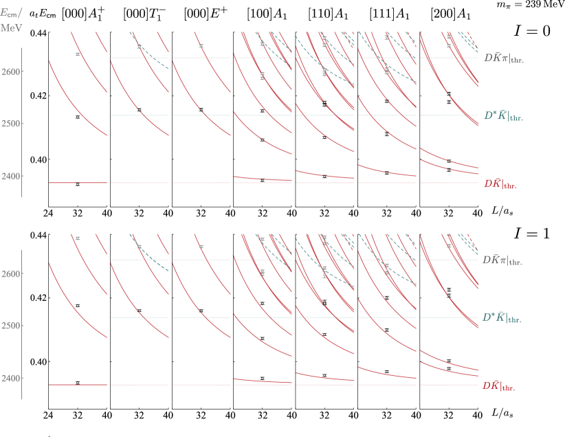
Figure 5: As Figure 3 but for $I=0$ and $I=1$ $D\bar{K}$ on the $m_{\pi}=239$ MeV ensemble.

4.4 $D\bar{K}$ $I=0,1$ with $m_{\pi}=391$ MeV

Finite-volume spectra for $D\bar{K}$ with $I=0$ and $I=1$ on the $m_{\pi}=391$ MeV ensemble, computed using the operators listed in Table 9, are shown in Figs. 6 and 7 respectively. These spectra show the same qualitative features as those on the $m_{\pi}=239$ MeV ensemble in Fig. 5. In the scattering analyses we use the energy levels shown in black in the figures – these are levels below the lowest non-interacting $D^{\ast}\bar{K}$ energy level. Some representative examples of the underlying principal correlator fits are again given in Appendix B.

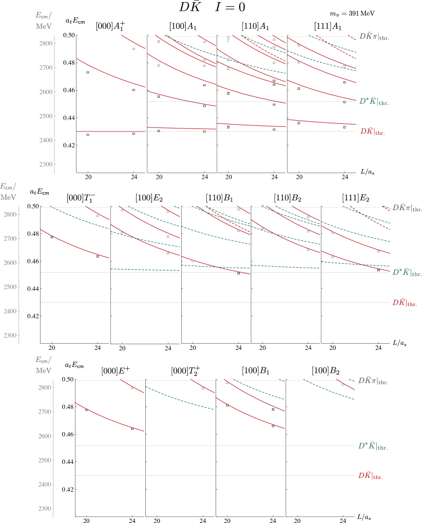
Figure 6: As Figure 3 but for $I=0$ $D\bar{K}$ on the $m_{\pi}=391$ MeV ensembles.

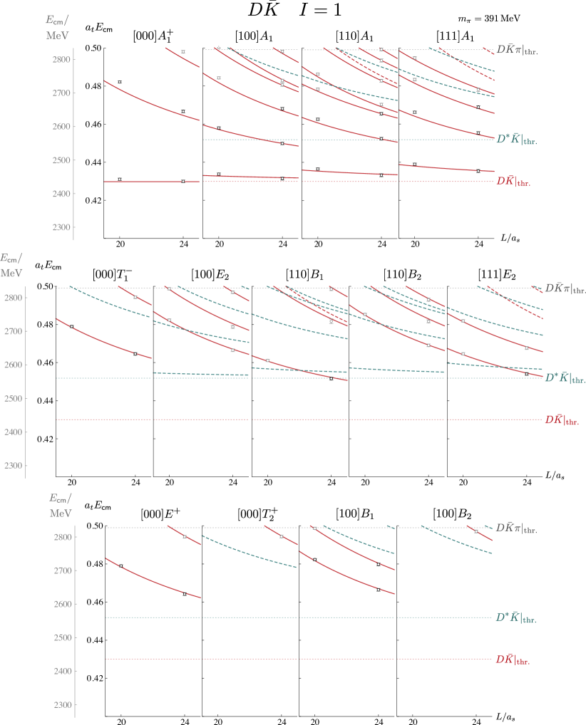
Figure 7: As Figure 3 but for $I=1$ $D\bar{K}$ on the $m_{\pi}=391$ MeV ensembles.

5 Scattering amplitudes

Infinite-volume scattering amplitudes are related to finite-volume energy levels through a quantisation condition derived by Lüscher and subsequently extended by many others. For the case of elastic hadron-hadron scattering, the quantisation condition Luscher:1986pf ; Luscher:1990ux ; Luscher:1991cf ; Rummukainen:1995vs ; Kim:2005gf ; Christ:2005gi ; Fu:2011xz ; Leskovec:2012gb ; Briceno:2014oea for lattice irrep $\Lambda$ with overall momentum $\vec{P}$ can be written as,

$$\det\left[\delta_{\ell\ell^{\prime}}\delta_{nn^{\prime}}+i\,\rho(E_{\mathsf{cm}})\,t^{(\ell)}(E_{\text{cm}})\left(\delta_{\ell\ell^{\prime}}\delta_{nn^{\prime}}+i\,\mathcal{M}^{\vec{P},\Lambda}_{\ell n;\ell^{\prime}n^{\prime}}(E_{\mathsf{cm}},L)\right)\right]=0\,,$$ (2)

where the determinant is over $\ell$, the partial waves which subduce into $\Lambda$, and $n$, indexing the embeddings of $\ell$ in $\Lambda$; the pattern of subductions is shown in Table 3. Here $\rho(E_{\mathsf{cm}})=2k/E_{\mathsf{cm}}$ is the phase space, $E_{\mathsf{cm}}$ and $k$ are the energy and momentum in the centre-of-momentum ($\mathsf{cm}$) frame, and $t^{(\ell)}$ is the infinite-volume $t$-matrix in partial wave $\ell$, which for elastic scattering can be written in terms of a single energy-dependent scattering phase-shift, $\delta_{\ell}(E_{\text{cm}})$, as $t^{(\ell)}=\tfrac{1}{\rho}e^{i\delta_{\ell}}\sin\delta_{\ell}$. The volume-dependent matrix of known functions of energy, $\mathcal{M}^{\vec{P},\Lambda}_{\ell n;\ell^{\prime}n^{\prime}}$, is not diagonal in partial waves, a manifestation of the reduced symmetry of a finite cubic volume. Ref. Briceno:2017max reviews this formalism and its application to the determination of elastic and coupled-channel scattering amplitudes.

In principle, an infinite set of partial waves contributes to the finite-volume spectrum in each irrep and the determinant in Eq. 2 is over an infinite-dimensional space. However, the kinematic suppression of higher partial waves close to threshold (in the absence of any dynamical enhancement) enables us to consider only the lower partial waves which contribute to each irrep. If, in a particular energy region, only one partial wave is relevant for a given irrep, Eq. 2 gives a one-to-one relation between each energy level, $E_{\mathsf{cm}}$, and the scattering $t$-matrix (or phase shift) at that energy.

When more than one partial wave is relevant there is no longer a one-to-one mapping between energy levels and phase shifts. We will follow the the approach of Ref. Dudek:2012gj where the energy dependence of the $t$-matrix is parametrised in terms of a small number of parameters and the best fit to the extracted finite-volume spectra is found by varying the parameters, minimising a $\chi^{2}$ function (Eq. (9) in Ref. Dudek:2012xn ). In order to ensure that results are not biased by a particular choice of parametrisation, we consider a variety of different forms.

One parametrisation of the $t$-matrix for elastic scattering is the effective range expansion, an expansion about threshold, given by,

$$k^{2\ell+1}\cot\delta_{\ell}=\frac{1}{a_{\ell}}+\frac{1}{2}r_{\ell}k^{2}+\mathcal{O}(k^{4})\,,$$ (3)

where the parameters $a_{\ell}$ and $r_{\ell}$ are known as the scattering length and the effective range. The scattering-length parametrisation corresponds to setting $r_{\ell}=0$. Another form, commonly used to parametrise a narrow resonance, is the relativistic Breit-Wigner,

$$t^{(\ell)}(s)=\frac{1}{\rho(s)}\frac{\sqrt{s}\Gamma_{\ell}(s)}{m_{R}^{2}-s-i\sqrt{s}\Gamma_{\ell}(s)}\,$$ (4)

where $s=E^{2}_{\text{cm}}$, the width, $\displaystyle\Gamma_{\ell}(s)=\frac{g_{R}^{2}}{6\pi}\frac{k^{2\ell+1}}{s\,m_{R}^{2(\ell-1)}}$, ensures the correct threshold behaviour, and the parameters are the Breit-Wigner mass, $m_{R}$, and the coupling constant, $g_{R}$.

A more general approach is to write the $t$-matrix in terms of a real symmetric $K$-matrix,

$$t^{-1}(s)=\frac{1}{(2k)^{\ell}}K^{-1}(s)\frac{1}{(2k)^{\ell}}+I(s)\,,$$ (5)

where for brevity we have dropped the partial-wave label $\ell$. Unitarity of the $S$-matrix is guaranteed if $\text{Im}[I(s)]=-\rho(s)$ above threshold and zero below. There is some remaining freedom in choosing $I$ and one of the simplest choices is $I(s)=-i\rho(s)$. Another choice is the Chew-Mandelstam prescription Chew:1960iv that defines $\text{Re}[I(s)]$ in terms of a dispersive integral and has a better analytic structure and a smoother transition across threshold; our implementation is described in Ref. Wilson:2014cna . This is a particularly convenient class of parametrisations for inelastic scattering, where $K$ is a matrix, but can equally be used to give a variety of forms for elastic scattering where $K$ is a real function.

We parametrise $K$ in terms of a pole and a polynomial,

$$K(s)=\left(\sum^{N_{g}}_{n=0}g^{(n)}s^{n}\right)^{2}\frac{1}{m^{2}-s}+\sum^{N_{\gamma}}_{n=0}\gamma^{(n)}s^{n}\,,$$ (6)

where $g^{(n)}$, $\gamma^{(n)}$ and $m$ are real parameters, or $K^{-1}$ in terms of a polynomial,

$$[K(s)]^{-1}=\sum^{N_{c}}_{n=0}c^{(n)}s^{n}\,,$$ (7)

where $c^{(n)}$ are real parameters. When we use the Chew-Mandelstam prescription, we will subtract at the $K$-matrix pole at $s=m^{2}$ when present or at threshold when there is no $K$-matrix pole term.

We now determine scattering amplitudes on the $m_{\pi}=239$ and $m_{\pi}=391$ MeV ensembles using the extracted finite-volume energy levels described above. Our discussion begins with $I=0$ $DK$ scattering before moving on to the flavour-exotic $I=0$ and $1$ $D\bar{K}$-channels. In Section 6 we then analytically continue these amplitudes into the complex energy plane to find the location of pole singularities and interpret the results.

5.1 $DK$ scattering in $I=0$

Starting with the $m_{\pi}=239$ MeV ensemble, we analyse the 22 energy levels shown in black in Fig. 3 – these are below $D^{\ast}K$ threshold in the $A_{1}^{+}$ and $A_{1}$ irreps where the lowest contribution is from $\ell=0$, and below $D_{s}\pi\pi$ threshold in other irreps where the lowest contribution is from $\ell=1$. For now we neglect partial waves with $\ell\geq 2$, but we return to this point in Section 5.1.2. A good fit to the spectra is obtained using a $K$-matrix parametrisation with a pole in $\ell=0$ and a pole plus a constant term in $\ell=1$, with Chew-Mandelstam phase space,

$m_{0}\;\;=$	$(0.38868\pm 0.00029\,^{+\,0.00004}_{-\,0.00003})\cdot a_{t}^{-1}$	$\begin{bmatrix}1&0.61&0.62&-0.17&-0.50\\ &1&0.40&-0.15&-0.48\\ &&1&-0.40&-0.59\\ &&&1&0.79\\ &&&&1\\ \end{bmatrix}$
$g^{(0)}_{0}\;\;=$	$(0.629\pm 0.053\,^{+\,0.009}_{-\,0.008})\cdot a_{t}^{-1}$
$m_{1}\;\;=$	$(0.34432\pm 0.00014\pm 0.00002)\cdot a_{t}^{-1}$
$g^{(0)}_{1}\;\;=$	$2.94\pm 0.37\,^{+\,0.03}_{-\,0.21}$
$\gamma^{(0)}_{1}\;\;=$	$(119\pm 69\,^{+\,10}_{-\,23})\cdot a_{t}^{2}$
	$\chi^{2}/N_{\mathrm{dof}}=\frac{15.1}{22-5}=0.89,$

(8)

where the subscript on the parameters labels the partial wave, $\ell$, the first uncertainty is statistical, and the second is an envelope over the uncertainties from varying the $D$ and $K$ meson masses and the anisotropy within their uncertainties. The matrix on the right gives the correlations between the parameters.

Similarly, on the $m_{\pi}=391$ MeV ensemble we analyse the 34 energy levels in irreps where the lowest contribution is from $\ell=0$ or $1$, the black points in the top two rows of Fig. 4. A reasonable fit to the data is again obtained using a $K$-matrix parametrisation with a pole in $\ell=0$ and a pole plus a constant term in $\ell=1$, with Chew-Mandelstam phase space,

$m_{0}\;\;=$	$(0.41981\pm 0.00029\,^{+\,0.00001}_{-\,0.00002})\cdot a_{t}^{-1}$	$\begin{bmatrix}1&0.47&0.71&-0.35&-0.52\\ &1&0.33&-0.19&-0.14\\ &&1&-0.65&-0.71\\ &&&1&0.87\\ &&&&1\\ \end{bmatrix}$
$g^{(0)}_{0}\;\;=$	$(0.536\pm 0.019\,^{+\,0.022}_{-\,0.006})\cdot a_{t}^{-1}$
$m_{1}\;\;=$	$(0.36564\pm 0.00019\,^{+\,0.00002}_{-\,0.00001})\cdot a_{t}^{-1}$
$g^{(0)}_{1}\;\;=$	$0.72\pm 0.82\,^{+\,0.03}_{-\,0.07}$
$\gamma^{(0)}_{1}\;\;=$	$(58\pm 25\,^{+\,8}_{-\,7})\cdot a_{t}^{2}$
	$\chi^{2}/N_{\mathrm{dof}}=\frac{45.4}{34-5}=1.56.$

(9)

In Fig. 8 we show a comparison between the computed finite-volume energy levels and the energy levels which follow from Eq. (9) using the quantisation condition, Eq. (2). This demonstrates the good description of the data provided by the parametrisation, reflecting the reasonable $\chi^{2}/N_{\mathrm{dof}}$ of the fit. It also shows the good description of computed energy levels below $D_{s}\eta$ threshold which were not used in the fit (grey points), with the exception of those above $DK$ threshold in the lower row which are expected to be $J^{P}=1^{+}$ (and/or higher $J$) and so not described by $S$ and $P$-wave $DK$ amplitudes.

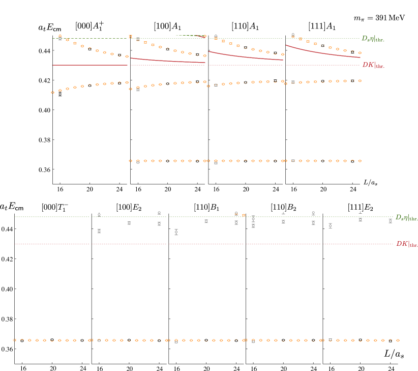
Figure 8: $DK$ $I=0$ finite-volume spectra on the $m_{\pi}=391$ MeV ensembles, as in the top two rows of Fig. 4, with the addition of orange points which show the energy levels from the parametrisation in Eq. (9).

The amplitudes for $m_{\pi}=239$ MeV and $m_{\pi}=391$ MeV presented in Eqs. (8) and (9), which we refer to as reference parametrisations, are shown in Fig. 9. The figure also shows the good agreement between the computed finite-volume energy levels and the energy levels from these parametrisations. It can be seen that, while there is a significant amplitude for scattering in $S$ wave, the $P$-wave amplitude is close to zero for physical scattering energies. There is an energy level very far below threshold in irreps where the lowest contribution is from $P$-wave scattering with an energy that shows very little dependence on the volume or irrep, suggestive of a $J^{P}=1^{-}$ bound state. Because this bound state is far below threshold, it does not appear to influence the physical $DK$ scattering region strongly.

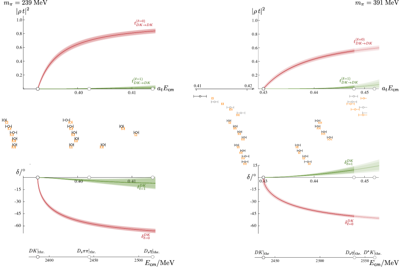
Figure 9: $S$ and $P$-wave squared-amplitudes (upper) and scattering phase shifts (lower) for $I=0$ $DK$ on the $m_{\pi}=239$ MeV (left) and $m_{\pi}=391$ MeV (right) ensembles. The darker inner bands are the reference parametrisations given in Eqs. (8) and (9) with statistical uncertainties, while the lighter outer bands reflect the uncertainty from varying the $D$ and $K$ meson masses and the anisotropy as described in the text. The black points between the plots show the computed finite-volume energy levels from Section 4 used to constrain the amplitudes, grey points are finite-volume energy levels which were not used, and orange points show the energy levels following from the reference parametrisations.

A convenient alternative parametrisation for elastic scattering is the effective range expansion, Eq. (3). Using such a parametrisation in $S$-wave and a $K$-matrix with a pole plus a constant term in $P$-wave (as in the reference parameterisations) gives a good description of the finite-volume spectra for $m_{\pi}=239$ MeV,

$a_{0}\;\;=$	$(-43.6\pm 2.0\pm 0.5)\cdot a_{t}$	$\begin{bmatrix}&1&-0.77&-0.61&0.18&0.54\\ &&1&0.41&-0.16&-0.49\\ &&&1&-0.40&-0.59\\ &&&&1&0.79\\ &&&&&1\\ \end{bmatrix}$
$r_{0}\;\;=$	$(-0.79\pm 1.04\,^{+\,0.14}_{-\,0.20})\cdot a_{t}$
$m_{1}\;\;=$	$(0.34432\pm 0.00014\pm 0.00002)\cdot a_{t}^{-1}$
$g^{(0)}_{1}\;\;=$	$2.94\pm 0.34\,^{+\,0.05}_{-\,0.16}$
$\gamma^{(0)}_{1}\;\;=$	$(119\pm 69\,^{+\,10}_{-\,23})\cdot a_{t}^{2}$
	$\chi^{2}/N_{\mathrm{dof}}=\frac{15.1}{22-5}=0.89.$

(10)

The same parameterisation gives a reasonable description of the $m_{\pi}=391$ MeV spectra,

$a_{0}\;\;=$	$(-24.01\pm 0.53\,^{+\,0.48}_{-\,0.52})\cdot a_{t}$	$\begin{bmatrix}&1&-0.82&-0.64&0.33&0.42\\ &&1&0.35&-0.19&-0.15\\ &&&1&-0.65&-0.71\\ &&&&1&0.87\\ &&&&&1\\ \end{bmatrix}$
$r_{0}\;\;=$	$(-4.26\pm 0.62\,^{+\,0.64}_{-\,0.28})\cdot a_{t}$
$m_{1}\;\;=$	$(0.36564\pm 0.00019\,^{+\,0.00002}_{-\,0.00001})\cdot a_{t}^{-1}$
$g^{(0)}_{1}\;\;=$	$0.72\pm 0.82\,^{+\,0.03}_{-\,0.07}$
$\gamma^{(0)}_{1}\;\;=$	$(58\pm 25\,^{+\,8}_{-\,7})\cdot a_{t}^{2}$
	$\chi^{2}/N_{\mathrm{dof}}=\frac{45.6}{34-5}=1.57.$

(11)

5.1.1 Varying the parametrisations

The parametrisations used in Eq. (2) were varied to investigate how much dependence there is on the exact form chosen. The $K$-matrix type, in particular, can be used with a wide variety of different functional forms – we considered higher order polynomials, forms with and without explicit poles, and forms with and without Chew-Mandelstam phase-space. The amplitudes used and associated $\chi^{2}$’s are summarised in Table 4 – those parametrisations with a $\chi^{2}/N_{\mathrm{dof}}$ in italics are not considered an acceptable description of the data for the reason given in the table. We reject parametrisations which have a $\chi^{2}/N_{\mathrm{dof}}>1.6$, an additional level near the top of the fitted region which is not supported by the lattice QCD spectra, poles on the physical sheet located away from the real axis, or an additional finite-volume energy level below threshold. The scattering amplitudes from acceptable parametrisations are shown in Fig. 10. It can be seen that there is relatively little dependence on the particular form used in the energy region where we are constraining the amplitudes, but, as might be expected, there is more variation where we do not have constraints.

In Fig. 11 we present the $S$-wave scattering amplitudes as $a_{t}k\cot\delta_{\ell=0}$ for the reference amplitudes, the effective range parameterisations described above and a $K$-matrix pole plus constant form (parametrisations (aa), (x) and (a) in Table 4). This again shows that the amplitudes are relatively insensitive to the parametrisation chosen, though there is slightly more freedom in the shape of the amplitude for $m_{\pi}=391$ MeV around threshold, between the two clusters of constraints. Also plotted is $-|k|$ for $k^{2}<0$ – the intersection of this curve with $a_{t}k\cot\delta_{\ell=0}$ indicates the presence of a pole singularity in the scattering amplitude below $DK$ threshold on the real axis of the physical sheet. We examine the pole singularities of the amplitudes in more detail and discuss their interpretation in Section 6, but first we investigate a couple of partial waves which we have so far neglected.

Parametrisation	$N_{\mathrm{pars}}^{(\ell=0)}$	$N_{\mathrm{pars}}^{(\ell=1)}$	${m_{\pi}=239\>\mathrm{MeV}}$	${m_{\pi}=391\>\mathrm{MeV}}$
			$\chi^{2}/N_{\mathrm{dof}}$	$\chi^{2}/N_{\mathrm{dof}}$
			22 levels	34 levels
K-matrix with Chew-Mandelstam $I(s)$, $K_{1}=\frac{g_{1}^{2}}{m_{1}^{2}-s}+\gamma_{1}$,
(aa) $K=\frac{g^{2}}{m^{2}-s}$	2	3	0.89	1.56
(a)  $K=\frac{g^{2}}{m^{2}-s}+\gamma^{(0)}$	3	3	0.81	1.11
(b)  $K=\frac{g^{2}}{m^{2}-s}+\gamma^{(1)}s$	3	3	0.83	1.17
(c)  $K=\frac{(g^{(0)}+g^{(1)}s)^{2}}{m^{2}-s}$	3	3	0.81$\;{}^{\ddagger}$	1.08$\;{}^{\ddagger}$
(d)  $K^{-1}=c_{0}+c_{1}\hat{s}$	2	3	0.89	1.56
(e)  $K=(1+d_{1}\hat{s})/(c_{0}+c_{1}\hat{s})$	3	3	0.81	1.11
K-matrix with $I(s)=-i\rho(s)$ & $K_{1}=\frac{g_{1}^{2}}{m_{1}^{2}-s}+\gamma_{1}$
(f)  $K=\frac{g^{2}}{m^{2}-s}$	2	3	0.95	1.58
(g)  $K=\frac{g^{2}}{m^{2}-s}+\gamma^{(0)}$	3	3	0.91	1.36$\;{}^{\dagger}$
(h)  $K=\frac{g^{2}}{m^{2}-s}+\gamma^{(1)}s$	3	3	0.89$\;{}^{\dagger}$	1.45$\;{}^{\dagger}$
(i)  $K=\frac{(g^{(0)}+g^{(1)}s)^{2}}{m^{2}-s}$	3	3	0.88$\;{}^{\ddagger}$	1.32$\;{}^{\ddagger}$
(j)  $K^{-1}=c_{0}+c_{1}\hat{s}$	3	3	0.94	1.58
(k)  $K=(1+d_{0}\hat{s})/(c_{0}+c_{1}\hat{s})$	3	3	0.90$\;{}^{\ddagger}$	1.36$\;{}^{\dagger}$
K-matrix with Chew-Mandelstam $I(s)$ & $K_{1}=\frac{g_{1}^{2}}{m_{1}^{2}-s}$
(l)  $K=\frac{g^{2}}{m^{2}-s}$	2	2	0.93	2.03$\;{}^{\diamond}$
(m)  $K=\frac{g^{2}}{m^{2}-s}+\gamma^{(0)}$	3	2	0.84	1.09$\;{}^{\dagger}$
(n)  $K=\frac{g^{2}}{m^{2}-s}+\gamma^{(1)}s$	3	2	0.85	1.52
(o)  $K=\frac{(g^{(0)}+g^{(1)}s)^{2}}{m^{2}-s}$	3	2	0.83$\;{}^{\ddagger}$	1.06$\;{}^{\ddagger}$
(p)  $K^{-1}=c_{0}+c_{1}\hat{s}$	3	2	0.93	2.03$\;{}^{\diamond}$
(q)  $K=(1+d_{0}\hat{s})/(c_{0}+c_{1}\hat{s})$	3	2	0.83	1.09$\;{}^{\dagger}$
Effective range expansion in $\ell=0$ & $\ell=1$, $k^{2\ell+1}\cot\delta_{\ell}=$
(r)  $\frac{1}{a_{0}}$,  $\frac{1}{a_{1}}$	1	1	3.37$\;{}^{\diamond}$	3.72$\;{}^{\diamond}$
(s)  $\frac{1}{a_{0}}+\frac{1}{2}r_{0}k^{2}$,  $\frac{1}{a_{1}}$	2	1	2.36$\;{}^{\diamond}$	1.93$\;{}^{\diamond}$
(t)  $\frac{1}{a_{0}}$,  $\frac{1}{a_{1}}+\frac{1}{2}r_{1}k^{2}$	1	2	1.50	3.69$\;{}^{\diamond}$
(u)  $\frac{1}{a_{0}}+\frac{1}{2}r_{0}k^{2}$,  $\frac{1}{a_{1}}+\frac{1}{2}r_{1}k^{2}$	2	2	1.33	1.68$\;{}^{\diamond}$
(v)  $\frac{1}{a_{0}}+\frac{1}{2}r_{0}k^{2}+P_{2}k^{4}$,  $\frac{1}{a_{1}}+\frac{1}{2}r_{1}k^{2}$	3	2	0.92$\;{}^{\ddagger}$	1.18$\;{}^{\ddagger}$
(w)  $\frac{1}{a_{0}}+\frac{1}{2}r_{0}k^{2}$,  $\frac{1}{a_{1}}+\frac{1}{2}r_{1}k^{2}+P_{2}k^{4}$	2	3	1.40	1.61$\;{}^{\diamond}$
Effective range expansion in $\ell=0$ & $K_{1}=\frac{g_{1}^{2}}{m_{1}^{2}-s}+\gamma_{1}$ with Chew-Mandelstam $I(s)$
(x)  $k\cot\delta_{0}=\frac{1}{a}+\frac{1}{2}rk^{2}$	2	3	0.89	1.57
(y)  $k\cot\delta_{0}=\frac{1}{a}+\frac{1}{2}rk^{2}+P_{2}k^{4}$	3	3	0.81	1.13$\;{}^{\ddagger}$
Breit-Wigner in each partial waves
(z)   $t=\frac{1}{\rho}\frac{m\Gamma}{m^{2}-s-im\Gamma}$	2	2	1.28	2.09$\;{}^{\diamond}$

$\diamond$ – rejected due to high $\chi^{2}/N_{\mathrm{dof}}>1.6$
$\dagger$ – rejected due to an additional level near top of the fit region that is not supported by the data
$\ddagger$ – rejected due to physical-sheet complex poles or additional finite-volume level below threshold

Table 4: A selection of the $S$ and $P$-wave parametrisations used for elastic $I=0$ $DK$ scattering. $N^{(\ell)}_{\mathrm{pars}}$ indicates the number of free parameters for partial wave $\ell$. The $\chi^{2}/N_{\mathrm{dof}}$ in bold indicate the reference and effective range fits described in the text. Parametrisations with $\chi^{2}/N_{\mathrm{dof}}$ in italics are not considered an acceptable description of the data for the reason given in the table.

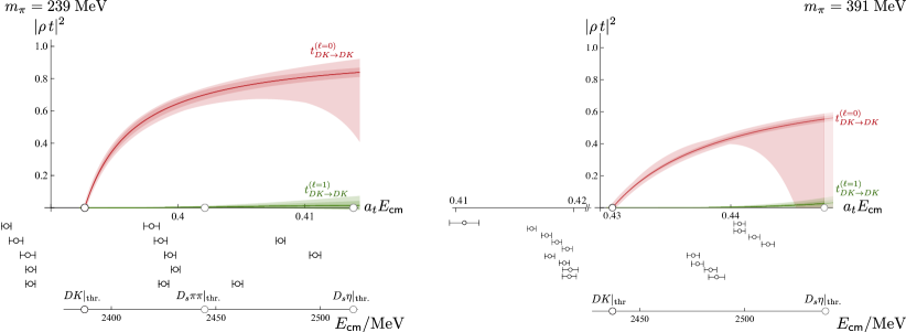
Figure 10: As in the upper plots in Fig. 9, but the lighter outer bands now also include an envelope over the acceptable parameterisations in Table 4 including their statistical uncertainties. The black points at the bottom show the computed finite-volume energy levels from Section 4 used to constrain the amplitudes.

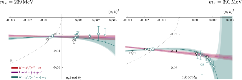
Figure 11: $DK$ $I=0$ $S$-wave scattering amplitudes, plotted as $a_{t}k\cot\delta_{\ell=0}$, using the reference (aa), effective range (x) and pole plus constant $K$-matrix (a) parametrisations for $m_{\pi}=239$ MeV (left) and $m_{\pi}=391$ MeV (right). Black points are determined from energy levels in the $[000]A_{1}^{+}$ irrep assuming $\ell>4$ amplitudes are negligible. Blue-green points are from the non-zero momentum $A_{1}$ irreps with amplitudes for higher partial waves fixed to zero.

5.1.2 $D$-wave scattering

Considering irreps where the lowest contribution is from $\ell=2$, on the ensemble with the lightest pion mass ($m_{\pi}=239$ MeV) there are no levels in the energy range where we can rigorously extract energies. For example, the lowest energy in the $[000]E^{+}$ irrep is above $D_{s}\pi\pi$ threshold as shown in Fig. 3. Nevertheless, the fact that this level is consistent with the non-interacting energy suggests that there is no significant $D$-wave $DK$ interaction below $D_{s}\eta$ threshold. Neglecting potential coupling to inelastic channels, that level corresponds to a scattering phase shift, $\delta_{2}=0.51(33)^{\circ}$. The results of Ref. Cheung:2016bym suggest that the lightest $2^{+}$ tensor resonance is at $a_{t}E\sim 0.43$, above the energy region we are considering.

The corresponding spectra for $m_{\pi}=391$ MeV are shown in the bottom row of Fig. 4. Although there are no energy levels below the $D_{s}\eta$ and $D^{\ast}K$ thresholds, there are a number which are well below the lowest non-interacting energies associated with these inelastic channels. The ‘extra’ level below the first non-interacting $DK$ energy, roughly consistent across volumes and irreps, is suggestive of a reasonably narrow resonance. A good description of the 10 levels shown in black in the bottom row of Fig. 4 is obtained using a relativistic Breit-Wigner parametrisation, Eq. (4),

$m_{R}\;\;=$	$(0.45578\pm 0.00052)\cdot a_{t}^{-1}$	$\begin{bmatrix}1&0.35\\ &1\\ \end{bmatrix}$
$g_{R}\;\;=$	$21.9\pm 2.4\,^{+2.0}_{-1.3}$
	$\chi^{2}/N_{\mathrm{dof}}=\frac{9.14}{10-2}=1.14,$

(12)

where, as usual, the first uncertainty is statistical and the second uncertainty on $g_{R}$ is from varying the $D$ and $K$ meson masses and the anisotropy (the uncertainty on $m_{R}$ from varying these is negligible). In Fig. 12 we show a comparison between the computed finite-volume energy levels and the energy levels which follow from this parametrisation. It can be seen that there is good agreement between the two sets of energy levels, reflecting the reasonable $\chi^{2}/N_{\mathrm{dof}}$ of the fit. Fig. 13 presents the amplitude following from this parametrisation. The phase shift is observed to rise steeply from near 0^∘ towards 180^∘, indicative of a narrow elastic resonance, and we examine the pole singularity in Section 6.

These results show that the $D$-wave amplitude is small in the energy region where we determined $S$ and $P$-wave amplitudes, justifying our neglect of $\ell\geq 2$ there.

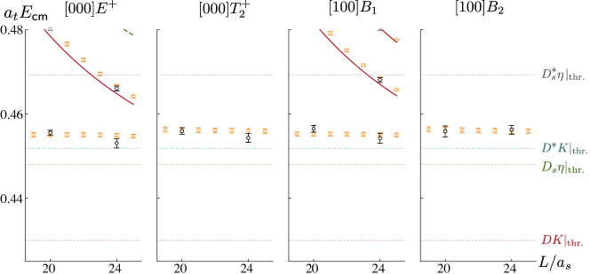
Figure 12: $DK$ $I=0$ finite-volume spectra on the $m_{\pi}=391$ MeV ensembles, as in the bottom row of Fig. 4 where black points indicate the computed finite-volume energy levels, with the addition of orange points which show the energy levels from the parametrisation in Eq. (12).

Figure 13: $D$-wave scattering phase shift for $I=0$ $DK$ on the $m_{\pi}=391$ MeV ensembles using the parametrisation in Eq. (12). The darker inner band indicates the statistical uncertainties, while the lighter outer band reflects the uncertainty from varying the $D$ and $K$ meson masses and the anisotropy as described in the text.

5.1.3 Positive-parity $J=1$ partial waves

Because of the reduced symmetry of the finite-volume lattice, $J^{P}=1^{+}$ can appear in $[100]E_{2}$, $[110]B_{1,2}$ and $[111]E_{2}$ irreps as well as $1^{-}$, with the lowest $1^{+}$ two-meson channel being $D^{\ast}K$. On the $m_{\pi}=239$ MeV ensemble, the results of Ref. Cheung:2016bym suggest that two $1^{+}$ axial-vector resonances should be expected at $a_{t}E\sim 0.41$ – $0.42$. We included a few $D^{\ast}K$-like operators in the operator bases for these irreps, as shown in Table 6. The finite-volume spectra in Fig. 3 have several levels in the vicinity of $D^{\ast}K$ threshold which have significant overlap with both $D^{\ast}K$ and fermion-bilinear operators, where the latter are subduced from $1^{+}$. One of these appears to be an ‘extra’ level at $a_{t}E\sim 0.41$, below $D^{\ast}K$ threshold, with the possibility of another a bit higher in energy.

Considering the first excited levels in $[100]E_{2}$ and $[110]B_{2}$ which have dominant overlap with $D^{\ast}K$ operators and fermion-bilinear operators subduced from $J^{P}=1^{+}$, we can make a rough estimate of the $J^{P}=1^{+}$ amplitude. The $[100]E_{2}$ level is found at $a_{t}E_{\mathsf{cm}}=0.4087(4)$ corresponding to $a_{t}k\cot\delta=-0.0233(14)$, and the $[110]B_{2}$ level is found at $a_{t}E_{\mathsf{cm}}=0.4088(5)$ corresponding to $a_{t}k\cot\delta=-0.0242(14)$. These values imply large negative scattering lengths ($a_{1^{+}}\approx-40a_{t}$), usually indicative of a near-threshold pole. Introducing a $D^{\ast}K$ $J^{P}=1^{+}$ amplitude with such a scattering length has negligible impact on the extraction of the $DK$ $1^{-}$ amplitude and thus on our determination of the $DK$ $0^{+}$ amplitude.

A similar pattern is observed on the ensembles with $m_{\pi}=391$ MeV when comparing with spectra obtained using only fermion-bilinear operators Moir:2013ub . From this and the expected masses of the lightest axial-vector resonances, we expect the $D^{\ast}K$ $1^{+}$ amplitude to again have a negligible impact on our extraction of the $DK$ $1^{-}$ and $0^{+}$ amplitudes. However, no $D^{\ast}K$ operators were used here and so we cannot estimate the size of this $D^{\ast}K$ $1^{+}$ amplitude.

5.2 $D\bar{K}$ scattering in $I=0$

Compared to the $DK$ scattering amplitudes discussed above, the spectra in Figs. 5, 6 and 7 suggest that the interactions in the exotic-flavour $D\bar{K}$ channels are relatively weak, with a slight attraction and repulsion in, respectively, $I=0$ and $I=1$. When meson-meson interactions are weak, as they are in these channels, we find that the correlations between different finite-volume energy levels on the same volume can be considerable. To assess a possible impact from imprecisely estimating these correlations, we perform some “covariance-adjusted” fits where the eigenvalues, $\lambda$, of the data correlation matrix for which $\lambda<r\lambda_{\textrm{max}}$ are replaced by $r\lambda_{\textrm{max}}$, where $\lambda_{\textrm{max}}$ is the largest eigenvalue; our default fit corresponds to $r=0$.

To start our analysis of isospin-0 $D\bar{K}$ on the $m_{\pi}=239$ MeV ensemble, we consider only the lowest 6 energy levels near threshold from irreps where the leading contribution is $S$-wave scattering. Fitting to an $S$-wave scattering length gives $a_{0}/a_{t}=4.9\pm 3.8$ with $\chi^{2}/N_{\mathrm{dof}}=5.0/5=1.0$.

Expanding the energy range, we fit the 18 levels which are well below the lowest $D^{\ast}\bar{K}$ non-interacting energy; these are the black points in Fig. 5. A good description of the data is obtained with an effective range parametrisation in $S$-wave, and a scattering length in $P$-wave and $D$-wave,

$a_{0}/a_{t}\;\;=$	$9.4\pm 1.8\,^{+\,0.8}_{-\,0.5}$	$\begin{bmatrix}&1&0.92&0.59&0.45\\ &&1&0.30&0.24\\ &&&1&0.73\\ &&&&1\end{bmatrix}$
$r_{0}/a_{t}\;\;=$	$32\pm 11\,^{+\,4}_{-\,2}$
$a_{1}/a_{t}^{3}\;\;=$	$-75\pm 90\pm 42$
$a_{2}/a_{t}^{5}\;\;=$	$-15200\pm 8100\pm 5500$
	$\chi^{2}/N_{\mathrm{dof}}=\frac{11.4}{18-4}=0.81$,

(13)

where, as usual, the first uncertainty is statistical. The second uncertainty is an envelope over the uncertainties from varying the $D$ and $\bar{K}$ meson masses and the anisotropy, as well as the uncertainty from a covariance-adjusted fit with $r=0.002$. Details of covariance-adjusted fits with $r=0.001$, $0.002$, $0.005$ and $0.01$ are given in Table 11 in Appendix C – these show that the central values of the fit parameters do not change significantly as $r$ is increased, while the uncertainties increase slightly. For comparison, that table also shows a fit where correlations between energy levels have been ignored.

The phase shifts resulting from this parametrisation are presented in Fig. 14 (top left plot). The figure also shows the good agreement between the computed finite-volume energy levels and the energy levels which follow from this parametrisation, reflecting the reasonable $\chi^{2}/N_{\mathrm{dof}}$ of the fit.

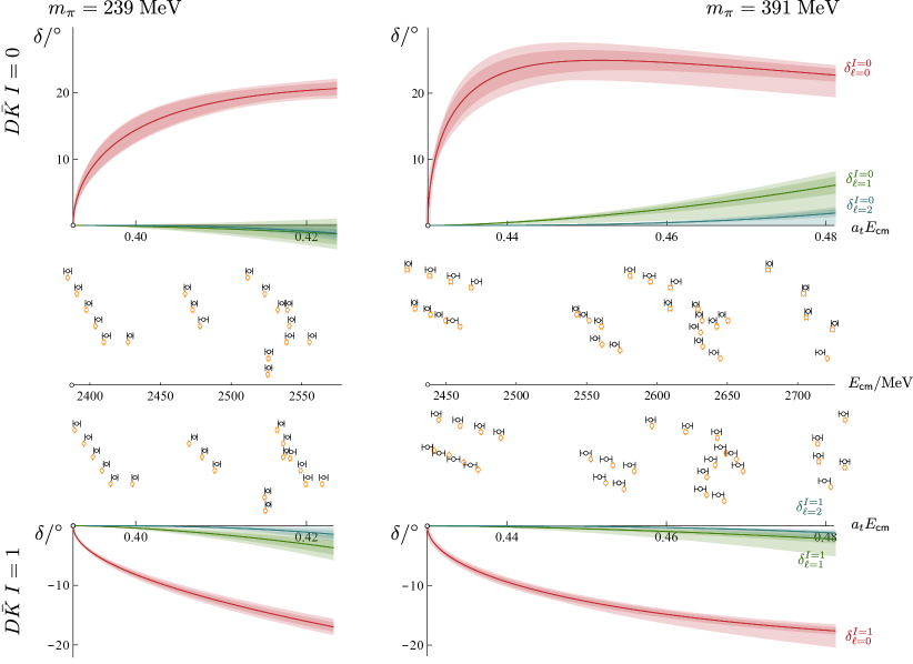
Figure 14: $S$, $P$ and $D$-wave scattering phase shifts for $D\bar{K}$ in $I=0$ (upper) and $I=1$ (lower) on the $m_{\pi}=239$ MeV (left) and $m_{\pi}=391$ MeV (right) ensembles. The darker inner bands are the reference parametrisations given in Eqs. (13), (14), (15) and (16) with statistical uncertainties, while the lighter outer bands give an envelope over the uncertainties from varying the $D$ and $\bar{K}$ meson masses and the anisotropy within their uncertainties, as well as a covariance-adjusted fit as described in the text with its statistical uncertainty. The black points in the middle show the computed finite-volume energy levels from Section 4 used to constrain the amplitudes, while the orange points show the energy levels following from the reference parametrisations.

On the $m_{\pi}=391$ MeV ensembles, fitting only the lowest energy level in each irrep where the leading contribution is from $S$-wave scattering (8 levels in total) to an $S$-wave scattering length gives $a_{0}/a_{t}=16.5\pm 3.1$ with $\chi^{2}/N_{\mathrm{dof}}=8.9/7=1.3$.

Opening up the energy range, we fit the 29 levels shown as black points in Fig. 6. A good description is obtained with an effective range parametrisation in $S$-wave, and a scattering length in $P$-wave and $D$-wave,

$a_{0}/a_{t}\;\;=$	$15.8\pm 2.2\,^{+\,1.9}_{-\,1.5}$	$\begin{bmatrix}&1&0.41&0.73&0.75\\ &&1&-0.11&-0.10\\ &&&1&0.98\\ &&&&1\end{bmatrix}$
$r_{0}/a_{t}\;\;=$	$36.5\pm 1.8\,^{+\,7.2}_{-\,1.5}$
$a_{1}/a_{t}^{3}\;\;=$	$128\pm 26\,^{+\,19}_{-\,63}$
$a_{2}/a_{t}^{5}\;\;=$	$4500\pm 1300\,^{+\,800}_{-\,3100}$
	$\chi^{2}/N_{\mathrm{dof}}=\frac{19.3}{29-4}=0.77$.

(14)

The phase shifts resulting from this parametrisation are shown in Fig. 14 (top right plot), along with a comparison between the computed energy levels and those which follow from the parametrisation. Covariance-adjusted fits are presented in Table 12 in Appendix C and, again, show that the results are insensitive to the value of $r$.

To avoid the results being biased by a particular choice, we varied the $S$-wave parametrisation, making use of higher orders in the effective range expansion and using various $K$-matrix amplitudes with simple or Chew-Mandelstam phase-space. For the $P$ and $D$-wave amplitudes we use either a scattering length or a constant $K$-matrix. Results are summarised in Table 5 – those parametrisations with a $\chi^{2}/N_{\mathrm{dof}}$ in italics are not considered an acceptable description of the data for the reason given in the table. The scattering amplitudes from acceptable parametrisations are shown in Fig. 15 where it can be seen that there is relatively little difference between the form of the amplitudes in the energy region where we are constraining the parametrisations.

As an alternative presentation of the $S$-wave scattering amplitudes, Fig. 16 shows $a_{t}k\cot\delta_{\ell=0}$ in the region around $D\bar{K}$ threshold. Also shown is $|k|$ for $k^{2}<0$ – the intersection of this curve with $a_{t}k\cot\delta_{\ell=0}$ indicates the presence of a pole singularity below threshold on the real axis of the unphysical sheet, and we examine this in Section 6.

				$m_{\pi}=239$ MeV		$m_{\pi}=391$ MeV
Parametrisation details				$\chi^{2}/N_{\mathrm{dof}}$	$\chi^{2}/N_{\mathrm{dof}}$	$\chi^{2}/N_{\mathrm{dof}}$	$\chi^{2}/N_{\mathrm{dof}}$
				$I=0$	$I=1$	$I=0$	$I=1$
$P$-wave and $D$-wave scattering lengths,
$S$-wave effective range expansion:
(a)	$\frac{1}{a}$			1.11	1.05	3.00$\;{}^{\diamond}$	1.74$\;{}^{\diamond}$
(b)	$\frac{1}{a}+\frac{1}{2}rk^{2}$			0.81	1.12	0.77	1.04
(c)	$\frac{1}{a}+\frac{1}{2}rk^{2}+P_{2}k^{4}$			0.86$\;{}^{\ddagger}$	1.05$\;{}^{\ddagger}$	0.75$\;{}^{\ddagger}$	0.88$\;{}^{\dagger}$
$K$-matrix with Chew-Mandelstam $I(s)$,
$P$-wave and $D$-wave with a constant $K$, $S$-wave with:
(d)	$K=\gamma^{(0)}$			0.94	1.05	2.48$\;{}^{\diamond}$	1.60$\;{}^{\diamond}$
(e)	$K=\gamma^{(0)}+\gamma^{(1)}s$			0.81	1.11	1.16	0.99
(f)	$K=\gamma^{(0)}+\gamma^{(1)}s+\gamma^{(2)}s^{2}$			0.86$\;{}^{\ddagger}$	1.03$\;{}^{\ddagger}$	0.88$\;{}^{\ddagger}$	0.89
(g)	$K^{-1}=c^{(0)}+c^{(1)}s$			0.82	1.12	0.78	1.04
$K$-matrix with simple phase space $I(s)=-i\rho(s)$,
$P$-wave and $D$-wave with a constant $K$, $S$-wave with:
(h)	$K=\gamma^{(0)}$			1.03	1.06	2.72$\;{}^{\diamond}$	1.30
(i)	$K=\gamma^{(0)}+\gamma^{(1)}s$			0.80	1.11	1.28	1.02
(j)	$K=\gamma^{(0)}+\gamma^{(1)}s+\gamma^{(2)}s^{2}$			0.86$\;{}^{\dagger}$	1.02$\;{}^{\ddagger}$	0.94$\;{}^{\ddagger}$	0.89
(k)	$K^{-1}=c^{(0)}+c^{(1)}s$			0.82	1.12	0.79	1.04

$\diamond$ – rejected due to high $\chi^{2}/N_{\mathrm{dof}}>1.5$
$\dagger$ – rejected due to high parameter correlations with parameter(s) consistent with zero
$\ddagger$ – rejected due to physical-sheet complex poles or additional finite-volume level below threshold

Table 5: A selection of the parametrisations used for elastic $D\bar{K}$ scattering with $I=0$ and $1$. The $\chi^{2}/N_{\mathrm{dof}}$ in bold indicate the reference fits which are described in the text. Parametrisations with $\chi^{2}/N_{\mathrm{dof}}$ shown in italics are not considered an acceptable description of the data for the reason given in the table.

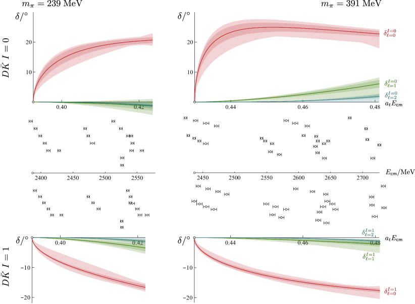
Figure 15: As Fig. 14, but the lighter outer bands now also include an envelope over the acceptable parameterisations in Table 5 including their statistical uncertainties. The black points in the middle show the computed finite-volume energy levels from Section 4 used to constrain the amplitudes.

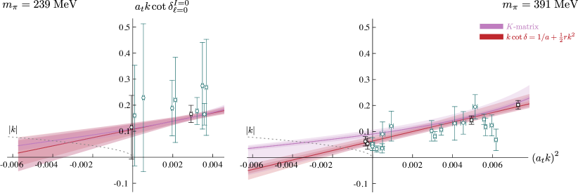
Figure 16: $S$-wave scattering amplitudes, plotted as $a_{t}k\cot\delta_{\ell=0}$, for $D\bar{K}$ in $I=0$ on the $m_{\pi}=239$ MeV (left) and $m_{\pi}=391$ MeV (right) ensembles. The bands show $K$-matrix parameterisation (e) in Table 5 and the reference effective range parameterisation, Eqs. (13) and (14), with their statistical uncertainties. Black points are determined from energy levels in the $[000]A_{1}^{+}$ irrep assuming $\ell>4$ amplitudes are negligible. Blue-green points are from the non-zero momentum $A_{1}$ irreps allowing for the $\ell=1$ amplitude which has been fixed from other irreps. Some points on the left plot with very large uncertainties have been removed.

5.3 $D\bar{K}$ scattering in $I=1$

Moving to isospin-1 $D\bar{K}$ on the $m_{\pi}=239$ MeV ensemble, fitting only the 6 lowest energy levels from irreps where the leading contribution is $S$-wave scattering to an $S$-wave scattering length gives $a_{0}/a_{t}=a=-4.4\pm 2.1$ with $\chi^{2}/N_{\mathrm{dof}}=8.0/5=1.6$. Expanding the energy range, we fit the 18 energy levels which are shown as black points in Fig. 5. A good description of the data is obtained with a scattering length parametrisation in $S$-wave, $P$-wave and $D$-wave,

$a_{0}/a_{t}\;\;=$	$-4.58\pm 0.23\,^{+0.15}_{-0.16}$	$\begin{bmatrix}&1&0.81&0.68\\ &&1&0.73\\ &&&1\end{bmatrix}$
$a_{1}/a_{t}^{3}\;\;=$	$-218\pm 68\,^{+53}_{-54}$
$a_{2}/a_{t}^{5}\;\;=$	$-19000\pm 8500\,^{+6700}_{-6900}$
	$\chi^{2}/N_{\mathrm{dof}}=\frac{15.7}{18-3}=1.05$.

(15)

The phase shifts resulting from this parametrisation are given in Fig. 14 (bottom left plot), along with a comparison between the computed energy levels and those which follow from the parametrisation. Covariance-adjusted fits are presented in Table 13 in Appendix C and show that, again, the central values do not change significantly when $r$ is increased, whereas uncertainties increase slightly.

On the $m_{\pi}=391$ MeV ensembles, if only the lowest energy level in each irrep where the leading contribution is from $S$-wave scattering (8 levels in total) is fitted to an $S$-wave scattering length, we obtain, $a_{0}/a_{t}=-2.9\pm 1.0$ with $\chi^{2}/N_{\mathrm{dof}}=6.1/7=0.87$. Using the full energy range, we fit the 28 energy levels shown as black points in Fig. 7. A good description is obtained with an effective range parametrisation in $S$-wave, and a scattering length in $P$-wave and $D$-wave,

$a_{0}/a_{t}\;\;=$	$-4.43\pm 0.30\,^{+0.12}_{-0.10}$	$\begin{bmatrix}&1&0.80&0.63&0.61\\ &&1&0.18&0.15\\ &&&1&0.95\\ &&&&1\end{bmatrix}$
$r_{0}/a_{t}\;\;=$	$-16.0\pm 3.2\,^{+8.6}_{-2.4}$
$a_{1}/a_{t}^{3}\;\;=$	$-47\pm 14\,^{+10}_{-46}$
$a_{2}/a_{t}^{5}\;\;=$	$-2800\pm 680\,^{+490}_{-2400}$
	$\chi^{2}/N_{\mathrm{dof}}=\frac{25.0}{28-4}=1.04$.

(16)

Fig. 14 (bottom right plot) shows the phase shifts resulting from this parametrisation along with a comparison between the computed energy levels and those which follow from the parametrisation. Covariance-adjusted fits are presented in Table 14 in Appendix C and, again, results show little dependence on $r$ with uncertainties increasing slightly as $r$ is increased.

In a similar way to $I=0$, we varied the $S$-wave parametrisation, using a scattering length or constant $K$-matrix for the $P$ and $D$-wave amplitudes. The results are summarised in Table 5 and the acceptable scattering amplitudes are shown in Fig. 15. It can be seen that there is relatively little variation between the amplitudes from different parametrisations in the energy region where we have data constraining them. In the following section we examine the pole singularities in the $DK$ and $D\bar{K}$ amplitudes, interpret the results and compare with previous work in the literature.

6 Poles, interpretation and comparisons

Once the scattering $t$-matrix has been determined, by analytically continuing into the complex $s=E^{2}_{\mathsf{cm}}$ plane, the location of pole singularities can be found and hence the bound-state and resonance content determined. For elastic scattering there is a branch point at threshold, with the usual approach taking a branch cut from threshold along the positive real axis, leading to two Riemann sheets labelled by the sign of the imaginary part of the momentum $k$. Bound states appear as poles lying on the real axis below threshold on the physical sheet ($\text{Im}[k]>0$). Poles that correspond to a resonance occur in complex-conjugate pairs on the unphysical sheet where $\text{Im}[k]<0$. In the proximity of a pole, the elastic $t$-matrix has the form,

$$t\sim\frac{c^{2}}{s_{\text{pole}}-s},$$ (17)

where $c$ gives the coupling of the pole to the scattering channel.

6.1 $S$ and $P$-wave $I=0$ $DK$

Analytically continuing the $S$ and $P$-wave isospin-0 $DK$ amplitudes, we find that, for both values of $m_{\pi}$, all the acceptable parametrisations have a pole on the real axis of the physical sheet below $DK$ threshold in the $S$-wave scattering amplitude, corresponding to a bound state. In $P$-wave there is a pole on the real axis of the physical sheet very far below threshold, corresponding to a deeply bound state. There are no other poles in the region where we are constraining the amplitudes.

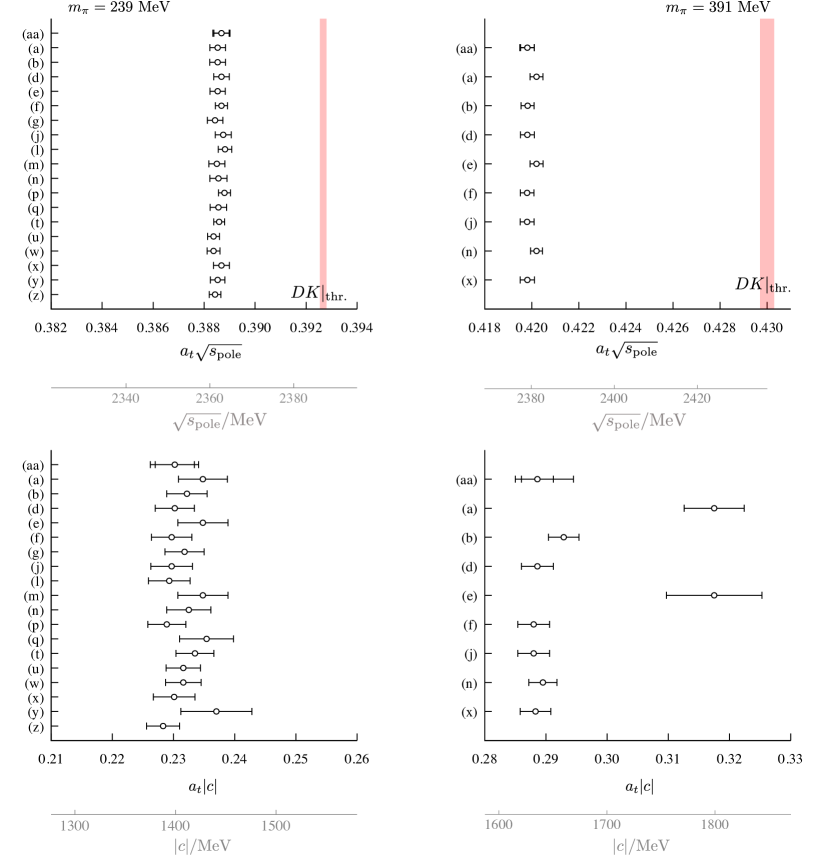
Figure 17: Upper: The location of the pole singularity on the real axis of the physical sheet in the $I=0$ $DK$ $S$-wave scattering amplitudes, for all the acceptable parametrisations in Table 4, on the $m_{\pi}=239$ MeV (left) and $m_{\pi}=391$ MeV (right) ensembles. The error bars give the statistical uncertainty, and the outer error bars on the reference amplitudes include also the uncertainty from varying the $D$ and $K$ meson masses and the anisotropy as described in the text. The red band shows the location of $DK$ threshold. Lower: The corresponding coupling, $|c|$.

The location of the $S$-wave pole and its coupling $c$, defined in Eq. (17), are presented in Fig. 17. The pole position is very insensitive to the choice of parametrisations, while the coupling for $m_{\pi}=391$ MeV is slightly more sensitive, reflecting the smaller constraint on the amplitude around threshold as seen in Fig. 11. As our final results for the pole position and coupling, we quote an envelope that spans the values from different parametrisations, including their statistical uncertainties,

	$m_{\pi}=239$ MeV	$m_{\pi}=391$ MeV
$a_{t}\sqrt{s_{\text{pole}}}\;\;=$	0.3886(5)	0.4200(5)
$a_{t}|c|\;\;=$	0.234(9)	0.305(20)
$\sqrt{s_{\text{pole}}}\;\;=$	2362(3) MeV	2380(3) MeV
$|c|\;\;=$	1420(50) MeV	1730(110) MeV.

This scalar bound state ($J^{P}=0^{+}$) has a large coupling to $DK$ and, at both $m_{\pi}$, its influence is strongly felt above threshold as seen in Fig. 10. The binding energy decreases with decreasing light-quark mass: $\Delta E=m_{D}+m_{K}-\sqrt{s_{\text{pole}}}=57(3)$ MeV for $m_{\pi}=391$ MeV and $\Delta E=25(3)$ MeV for $m_{\pi}=239$ MeV. It appears to correspond to the experimentally observed $D_{s0}^{\ast}(2317)$ which appears below $DK$ threshold with $\Delta E\approx 45$ MeV Tanabashi:2018oca – this is somewhat larger than our value on the ensemble with light-quark mass closest to the physical value. We note that there are unquantified systematic uncertainties in these calculations, such as discretisation effects Liu:2012ze ; Moir:2013ub ; Cheung:2016bym , which may contribute to this difference. In addition, experimentally the $D_{s0}^{\ast}(2317)$ is unstable and decays through the isospin-breaking $D_{s}\pi$ channel, whereas isospin symmetry is exact in our calculation.

We observe that the finite-volume eigenstates in the region of $DK$ threshold overlap significantly with both $c\bar{s}$ and $DK$-like operators; both structures appear to be essential in extracting the spectrum. While we do not use explicit compact-tetraquark operators in this calculation, extended four-quark components are present through the meson-meson operators. Given the proximity to threshold, one may question whether this state is composed primarily of a short-distance $c\bar{s}$ component or whether a longer-distance $DK$ component is dominant. One method to assess this from the scattering amplitude itself is the Weinberg compositeness condition Weinberg:1965zz , valid for weakly-bound states when the scattering hadrons interact in a relative $S$-wave. Assuming that the binding is weak enough so that corrections can be ignored,

$$a_{0}=-2\,\frac{1-Z}{2-Z}\,\frac{1}{\sqrt{2\,\mu\,\Delta E}}\,,\qquad r_{0}=-\,\frac{Z}{1-Z}\,\frac{1}{\sqrt{2\,\mu\,\Delta E}}\,,$$ (18)

where $0\leq Z\leq 1$, with $Z\approx 0$ indicating that a composite or molecular component dominates and $Z\approx 1$ indicating an elementary configuration, $\mu$ is the $DK$ reduced mass, $\Delta E$ is the binding energy, and $a_{0}$ and $r_{0}$ use the same conventions as in Eq. (3). Combining the two expressions to give $Z$ in terms of $a_{0}$ and $r_{0}$,

$$Z=1-\sqrt{\frac{a}{a+2r}}\,.$$ (19)

For $m_{\pi}=239$ MeV, $r_{0}$ is consistent with zero and supposing that the bound state is purely composite, $Z=0$, gives $a_{0}/a_{t}\approx-41$ to $-46$, consistent with Eq. (10). Alternatively, using the results in Eq. (10) and inverting the expressions for $a_{0}$ and $r_{0}$ in Eq. (18) gives $Z\lesssim 0.11$ and $Z\lesssim 0.04$ respectively, whereas Eq. (19) gives $Z\lesssim 0.04$. Performing the same analysis for $m_{\pi}=391$ MeV, assuming $Z=0$ (even though $r_{0}$ is not consistent with zero) gives $a_{0}/a_{t}\approx-25$ to $-26$, roughly consistent with Eq. (11). Instead using the results for $a_{0}$ and $r_{0}$ in Eq. (11) gives $Z\approx 0.13(6)$ and $Z\approx 0.14(3)$ respectively, whereas using Eq. (19) gives $Z\approx 0.14(3)$. This analysis suggests that a molecular $DK$ component dominates for both $m_{\pi}$.

Elastic $S$-wave $DK$ scattering has been studied by several other groups Mohler:2013rwa ; Lang:2014yfa ; Bali:2017pdv ; Alexandrou:2019tmk with a range of light-quark masses and lattice methodologies (see also re-analyses of lattice results in Torres:2014vna ; Guo:2018tjx ), and an earlier calculation Liu:2012zya computed the scattering length indirectly by using a chiral unitary approach to relate it to channels where there are no annihilation contributions. Broadly speaking, these calculation all find a bound-state pole and are consistent with a dominant $DK$ configuration. However, it is not straightforward to compare them because some have only dynamical light quarks with quenched strange quarks ($N_{f}=2$) rather than dynamical light and strange quarks ($N_{f}=2+1$), they use light-quark masses corresponding to different $m_{\pi}$, and some use very small volumes where corrections to the Lüscher quantisation condition may be significant. Ref. Alexandrou:2019tmk is the most directly comparable to our work with $N_{f}=2+1$, a reasonable volume ($m_{\pi}L\approx 4.4$) and $m_{\pi}=296$ MeV. They find a pole $\sim 51$ MeV below $DK$ threshold, consistent with our result for $m_{\pi}=391$ MeV, but somewhat larger than that for $m_{\pi}=239$ MeV.

For the $P$-wave deeply bound state, using a similar procedure we find a pole at,

	$m_{\pi}=239$ MeV	$m_{\pi}=391$ MeV
$a_{t}\sqrt{s_{\text{pole}}}\;\;=$	0.34432(22)	0.36579(43)
$\sqrt{s_{\text{pole}}}\;\;=$	2093(1) MeV	2073(2) MeV

This vector bound state ($J^{P}=1^{-}$) corresponds to the $D_{s}^{\ast}$ and does not appear to significantly influence $DK$ scattering in the physical scattering region. Its mass is consistent with the results obtained using only $\bar{q}q$ operators, see Section 3 and Refs. Liu:2012ze ; Cheung:2016bym , as expected for a state so far below threshold.

6.2 $D$-wave $I=0$ $DK$

The $D$-wave isospin-0 $DK$ amplitude on the $m_{\pi}=391$ MeV ensemble, Eq. (12), has a complex-conjugate pair of pole singularities on the unphysical sheet. They have,

$$a_{t}\sqrt{s_{\text{pole}}} = \bigl{(}0.4558\pm 0.0005\bigr{)}\pm\tfrac{i}{2}\bigl{(}0.0006\,^{+\,0.0003}_{-\,0.0002}\bigr{)}$$

$$a_{t}|c| = 0.033\,^{+\,0.007}_{-\,0.006}$$

$$\text{arg}[c] = \pm\left(0.0098\,^{+\,0.004}_{-\,0.003}\right)\pi$$

$$\sqrt{s_{\text{pole}}} = \bigl{(}2583\pm 3\bigr{)}\pm\tfrac{i}{2}\bigl{(}3.4\,^{+\,1.7}_{-\,1.1}\bigr{)}\text{MeV}$$

$$|c| = 190\,^{+\,40}_{-\,30}~{}\text{MeV}\,.$$

Any analogous pole on the $m_{\pi}=239$ MeV ensemble would be expected to be above the energy region where we can constrain the scattering amplitudes – there appears to be an extra level in the relevant irreps, suggesting a reasonably narrow resonance.

This tensor resonance ($J^{P}=2^{+}$) corresponds to the experimentally-observed $D^{\ast}_{s2}(2573)$. We find that its Breit-Wigner coupling, $g_{R}$, is similar to the $D^{\ast}_{2}$ resonance found in $D\pi$ scattering at the same pion mass in Ref. Moir:2016srx .

6.3 $I=0,1$ $D\bar{K}$

In $I=0$ $D\bar{K}$ scattering the $P$ and $D$-wave amplitudes are very small, but a sharper rise in the $S$-wave phase shift indicates that a virtual bound-state pole may be present, a pole on the real axis below threshold on the unphysical sheet, corresponding to an attractive interaction but one that is not strong enough to form a bound state. The $S$-wave $I=1$ channel appears to be weakly repulsive with $P$ and $D$-wave $I=1$ amplitudes roughly consistent with zero.

Analytically continuing the scattering amplitudes into the complex $s=E^{2}_{\mathsf{cm}}$ plane, we find that, for both $m_{\pi}$, most of the acceptable parametrisations do have a virtual bound-state pole below $D\bar{K}$ threshold in the $S$-wave $I=0$ scattering amplitude. There are no other poles in $I=0$ or $I=1$ $D\bar{K}$ in the region where the amplitudes are well-constrained.

The location and coupling $c$, defined in Eq. (17), of this exotic-flavour $J^{P}=0^{+}$ pole are presented in Fig. 18. The location is roughly consistent across parametrisations within statistical uncertainties, but there is somewhat more variation in the coupling. However, no pole is found for $m_{\pi}=239$ MeV on parametrisations (a), (d) and (h) which give a reasonable description of the finite-volume energy levels. We can therefore only say that there is a suggestion of a pole in the $I=0$ $D\bar{K}$ amplitudes, not that a pole is absolutely required. As our results for the position and coupling of this suggested pole, we quote an envelope that spans the values from different parametrisations where a pole is found, including their statistical uncertainties,

	$m_{\pi}=239$ MeV	$m_{\pi}=391$ MeV
$a_{t}\sqrt{s_{\text{pole}}}\;\;=$	0.357(23)	0.407(16)
$a_{t}|c|\;\;=$	0.26(7)	0.26(7).
$\sqrt{s_{\text{pole}}}\;\;=$	2170(140) MeV	2310(90) MeV
$|c|\;\;=$	1600(400) MeV	1500(400) MeV.

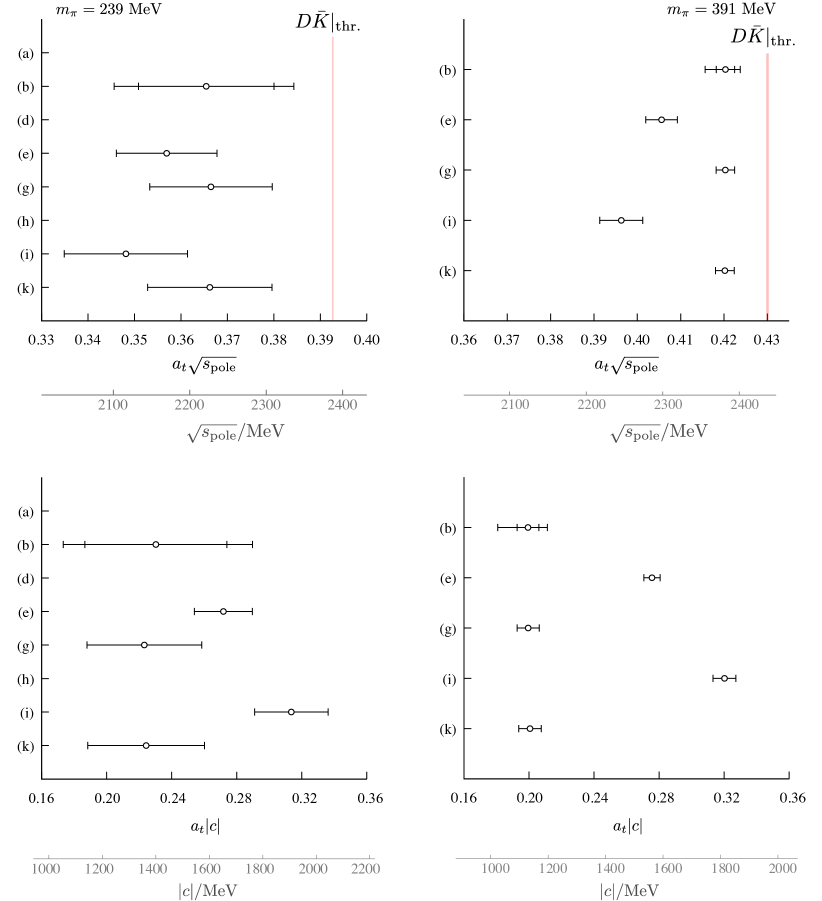
Figure 18: Upper: The location of the pole singularity on the real axis of the unphysical sheet in the $I=0$ $D\bar{K}$ $S$-wave scattering amplitudes, for acceptable parametrisations in Table 5, on the $m_{\pi}=239$ MeV (left) and $m_{\pi}=391$ MeV (right) ensembles. The error bars give the statistical uncertainty, and the outer error bars on the reference amplitudes include also the uncertainty from varying the $D$ and $K$ meson masses and the anisotropy, as well as a covariance-adjusted fit as described in the text. The red band shows the location of $D\bar{K}$ threshold. Lower: The corresponding coupling, $|c|$.

In some of the parameterisations used, a physical-sheet pole appears in the $I=0$ $D\bar{K}$ amplitudes at an energy much lower than the unphysical-sheet pole, well below where they are constrained by the finite-volume energy levels. The presence of this pole can be inferred from Fig. 16 where an intersection of the effective range curve, $1/a+\tfrac{1}{2}rk^{2}$, and $-|k|$ is inevitable at large negative $k^{2}$. Investigating further, we find that the residue of this pole has the “wrong” sign (see e.g. Sitenko:ScatteringTheory ; Taylor:ScatteringTheory ; Iritani:2017rlk ) and so signals that the amplitude is unphysical in this energy region – it has been extrapolated too far in energy from where it is being constrained. The $K$-matrix amplitude shown in Fig. 16 does not suffer this problem.

In Ref. Liu:2012zya , $S$-wave $D\bar{K}$ $I=0,1$ scattering lengths were computed for a range of $m_{\pi}$ using a partially-quenched lattice formulation. They found attraction in $I=0$ and repulsion in $I=1$, consistent with our results, but there was no suggestion of a virtual bound state in $I=0$. Our scattering-length parametrisation of $S$-wave $I=0$ scattering similarly does not lead to a virtual bound state in the region where we are constraining the amplitudes – we find that a form with at least two parameters is required to give a virtual bound state in this energy region.

Ref. Albaladejo:2016lbb found agreement between a unitarized chiral perturbation theory analysis of $D\pi$, $D\eta$, $D_{s}\bar{K}$ scattering and the lattice results in Ref. Moir:2016srx , and from this predicted the presence of a virtual bound state in $S$-wave $D\bar{K}$ $I=0$. Ref. Du:2017zvv goes further and, amongst other things, discusses how this state should appear at the SU(3) flavour symmetric point for various quark masses.

If the charm and strange quark masses were increased, this exotic-flavour $I=0$ $D\bar{K}$ $J^{P}=0^{+}$ channel would resemble an $I=0$ $bb\bar{u}\bar{d}$ system often considered as a possible tetraquark candidate. The related $J^{P}=1^{+}$ $I=0$ $bb\bar{u}\bar{d}$ systems have been observed to contain a bound state in lattice calculations Francis:2016hui ; Francis:2018jyb ; Junnarkar:2018twb ; Leskovec:2019ioa , but there was no evidence seen for a bound state in $J^{P}=1^{+}$ $I=0$ $cc\bar{u}\bar{d}$ in Ref. Cheung:2017tnt . Future investigations mapping out the mass, spin, and flavour dependence of these exotic systems will be particularly interesting.

6.4 $DK$, $D\bar{K}$ and $D\pi$ scattering and SU(3) flavour symmetry

In the limit of SU(3) flavour symmetry, where the up, down and strange quarks have the same mass, various channels in $DK$, $D\bar{K}$, $D\pi$, etc scattering are related. In the calculations presented here, the up and down quarks are degenerate and, particularly for the $m_{\pi}=391$ MeV ensembles, are not so much lighter than the strange quark. SU(3) may therefore not be too badly broken and provide a useful framework for interpreting the results.

The combination of a $D_{(s)}$ meson (SU(3) $\overline{\bm{3}}$) and a light meson ($\bm{8}$ or $\bm{1}$) gives,

$$\overline{\bm{3}}~{}\otimes~{}\bm{8}~{}\to~{}\overline{\bm{3}}~{}\oplus~{}\bm{6}~{}\oplus~{}\overline{\bm{15}}\,,\quad\overline{\bm{3}}\otimes\bm{1}\to\overline{\bm{3}}\,.$$

Using Ref. Kaeding:1995vq , the various scattering channels decompose into SU(3) multiplets as,

$(I=0)$ $DK$-$D_{s}\eta$: $\overline{\bm{3}}\oplus\overline{\bm{15}}$		$(I=\tfrac{1}{2})$ $D\pi$-$D\eta$-$D_{s}\bar{K}$: $\overline{\bm{3}}\oplus\bm{6}\oplus\overline{\bm{15}}$
$(I=1)$ $DK$-$D_{s}\pi$: $\bm{6}\oplus\overline{\bm{15}}$		$(I=0)$ $D\bar{K}$: ${\bm{6}}$
$(I=\tfrac{1}{2})$ $D_{s}K$, $(I=1)$ $D\bar{K}$, $(I=\tfrac{3}{2})$ $D\pi$: $\overline{\bm{15}}$

We found $S$-wave $D\bar{K}$ $(I=1)$ to be weakly repulsive with no poles in the energy region considered. This is very similar to the results for $D\pi$ $(I=3/2)$ presented in Ref. Moir:2016srx , consistent with them being identical in the SU(3) limit. We conclude that, in this energy region, $S$-wave $\overline{\bm{15}}$ exhibits weak repulsion and there are no poles in the scattering amplitude. From our results for $DK$ $(I=0)$, we conclude that the $S$-wave $\overline{\bm{3}}$ contains a bound state for the light-quark masses used here. From $D\bar{K}$ $(I=0)$, the $S$-wave $\bm{6}$ shows weak attraction and may contain a virtual bound state.

We would expect $D\pi$ $(I=1/2)$ to show behaviour which is a superposition of $DK$ $(I=0)$ and $D\bar{K}$ $(I=0)$, and so it could contain two poles. In Ref. Moir:2016srx , with $m_{\pi}=391$ MeV we found only one robustly-determined pole in $S$-wave $D\pi$ $(I=1/2)$ in the energy region considered, a bound state consistent in mass with the $D\pi$ threshold, but we did not exclude the possibility of another pole. This picture appears to have some similarity with Refs. Albaladejo:2016lbb ; Du:2017zvv ; Guo:2018tjx which suggest a “two-pole” structure in $I=1/2$ $D\pi$, $D\eta$, $D_{s}\bar{K}$, a bound-state pole and a resonance (complex-conjugate pair of poles) at $m_{\pi}=391$ MeV which evolve to two resonances for physical quark masses. Those references also discuss how states evolve as the quark masses are varied and related scattering channels; see Ref. Meissner:2020khl for a more general discussion of two-pole structures. The effect of SU(3) flavour symmetry breaking is apparent here: because $m_{K}>m_{\pi}$, the bound state in $DK$ is more bound than in $D\pi$. For physical light-quark masses we would expect even less binding in $D\pi$, consistent with experiment where the $D_{0}^{\ast}(2400)$ is a resonance rather than a bound state.

The $P$ and $D$-wave channels appear to be weakly interacting in the energy region we are considering, with the exception of the $\overline{\bm{3}}$ which contains a deeply bound state in $P$-wave and a narrow resonance in $D$-wave.

7 Summary and Outlook

Scattering amplitudes for $I=0$ $DK$ and $I=0,1$ $D\bar{K}$ have been determined using lattice QCD with light-quark masses corresponding to $m_{\pi}=239$ MeV and $m_{\pi}=391$ MeV. As described, the techniques we use enable us to reliably extract a large number of finite-volume energy levels and hence to map out precisely the energy dependence of the amplitudes in the elastic scattering region. Analytically continuing these amplitudes in the complex plane reveals the presence of a bound state in $S$-wave $I=0$ $DK$ and, for the first time in a lattice calculation, evidence for a virtual bound state in $S$-wave $I=0$ $D\bar{K}$. We summarise the $S$-wave poles found in this work in Fig. 19.

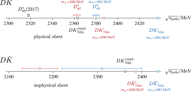
Figure 19: A summary of the $S$-wave poles found in this work. The top panel shows the bound-state poles found on the physical sheet in the $I=0$ $DK$ scattering amplitudes with the experimental $D_{s0}^{\ast}(2317)$ and threshold from Ref. Tanabashi:2018oca . The lower panel shows the virtual bound-state poles found on the unphysical sheet in the exotic $I=0$ $D\bar{K}$ scattering amplitudes; note that not all the amplitudes for $m_{\pi}=239$ MeV produced such a pole.

The $J^{P}=0^{+}$ $DK$ bound state, corresponding to the $D_{s0}^{\ast}(2317)$, is found close to $DK$ threshold: 57(3) MeV below threshold for the larger $m_{\pi}$, reducing to 25(3) MeV for the smaller $m_{\pi}$. It has a large coupling to the $DK$ channel and, as seen in Fig. 10, it leaves a clear signature on the elastic $DK$ scattering amplitude which rises sharply from threshold for both $m_{\pi}$. In $I=0$ $DK$ we also find a deeply bound vector in $P$-wave, corresponding to the $D_{s}^{\ast}$, and in addition there is some evidence for $2^{+}$ (see Fig. 13) and $1^{+}$ resonances at higher energies.

The exotic $I=0$ $D\bar{K}$ amplitudes are mapped out for the first time in a lattice calculation and we find that these interactions are smaller in magnitude than in $DK$ with only the $S$-wave determined to be significant, as shown in Fig. 15. As described above, we see hints of a $0^{+}$ $I=0$ virtual bound state pole below $D\bar{K}$ threshold – this is present in all the acceptable $m_{\pi}=391$ MeV amplitudes and the majority of those at $m_{\pi}=239$ MeV. The lighter pion mass produces an amplitude with larger uncertainties and more energies might constrain this better to produce a completely unambiguous result. The $I=1$ $D\bar{K}$ amplitudes are found to be weakly repulsive. It is interesting to note that lattice calculations have found signs of a bound state in similar $1^{+}$ $I=0$ exotic-flavour channels when the valence $c,s$-quarks are replaced by $b$-quarks Francis:2016hui ; Francis:2018jyb ; Junnarkar:2018twb ; Leskovec:2019ioa . Further calculations at a range of quark masses and in various flavour and spin channels would help map out the QCD dynamics at work in these systems.

The work described here opens the way to many possible avenues of exploration. For example, $D^{\ast}K$ amplitudes can be computed in an analogous way and a study of these would be particularly interesting since two $D_{s1}$ states are expected near $D^{\ast}K$ threshold – experimentally one is observed just below threshold and one just above threshold. More broadly, lattice calculations offer the possibility to map out the quark-mass dependence of the scattering amplitudes, yielding insight into the dynamics of QCD.

Appendices

Appendix A Operator Lists

In Tables 6, 7, 8 and 9 we list the interpolating operators used to determine the finite-volume energy levels in the $DK$ isospin-$0$ channel shown in Figs. 3 and 4, and the $D\bar{K}$ isospin-$0$ and $1$ channels shown in Figs. 5, 6 and 7.

$[000]A_{1}^{+}$	$[001]A_{1}$	$[011]A_{1}$	$[111]A_{1}$	$[002]A_{1}$
$D_{[000]}K_{[000]}$	$D_{[001]}K_{[000]}$	$D_{[011]}K_{[000]}$	$D_{[111]}K_{[000]}$	$D_{[002]}K_{[000]}$
$D_{[001]}K_{[001]}$	$D_{[000]}K_{[001]}$	$D_{[000]}K_{[011]}$	$D_{[000]}K_{[111]}$	$D_{[000]}K_{[002]}$
$D_{[011]}K_{[011]}$	$D_{[011]}K_{[001]}$	$D_{[001]}K_{[001]}$	$D_{[011]}K_{[001]}$	$D_{[001]}K_{[001]}$
$D_{[111]}K_{[111]}$	$D_{[001]}K_{[011]}$	$D_{[001]}K_{[111]}$	$D_{[001]}K_{[011]}$	$D_{[011]}K_{[011]}$
$D_{s[000]}\eta_{[000]}$	$D_{[002]}K_{[001]}$	$D_{[111]}K_{[001]}$	$D_{[112]}K_{[001]}$	$D_{[111]}K_{[111]}$
$D_{s[001]}\eta_{[001]}$	$D_{s[001]}\eta_{[000]}$	$D_{[011]}K_{[011]}$	$D_{s[111]}\eta_{[000]}$	$D_{[012]}K_{[001]}$
$D_{s[011]}\eta_{[011]}$	$D_{s[000]}\eta_{[001]}$	$D_{[012]}K_{[001]}$	$D_{s[011]}\eta_{[001]}$	$D_{s[002]}\eta_{[000]}$
	$D^{\ast}_{s[001]}f_{0[000]}$	$D_{s[011]}\eta_{[000]}$	$D^{\ast}_{[011]}K_{[001]}$	$D_{s[001]}\eta_{[001]}$
		$D_{s[001]}\eta_{[001]}$	$D^{\ast}_{s[111]}f_{0[000]}$	$D^{\ast}_{s[002]}f_{0[000]}$
		$D^{\ast}_{[001]}K_{[001]}$		$D^{\ast}_{s[001]}f_{0[001]}$
		$D^{\ast}_{s[011]}f_{0[000]}$
$({\bar{\psi}\mathbf{\Gamma}\psi})\times 18$	$({\bar{\psi}\mathbf{\Gamma}\psi})\times 32$	$({\bar{\psi}\mathbf{\Gamma}\psi})\times 52$	$({\bar{\psi}\mathbf{\Gamma}\psi})\times 36$	$({\bar{\psi}\mathbf{\Gamma}\psi})\times 32$

$[000]T_{1}^{-}$	$[000]E^{+}$	$[001]E_{2}$	$[011]B_{1}$	$[011]B_{2}$	$[111]E_{2}$
$D_{[001]}K_{[001]}$	$D_{[001]}K_{[001]}$	$D_{[001]}K_{[011]}$	$D_{[001]}K_{[001]}$	$D_{[111]}K_{[001]}$	$D_{[011]}K_{[001]}$
$D_{[011]}K_{[011]}$	$D_{[011]}K_{[011]}$	$D_{[011]}K_{[001]}$	$D_{[012]}K_{[001]}$	$D_{[011]}K_{[011]}$	$D_{[001]}K_{[011]}$
$D_{s[001]}\eta_{[001]}$	$D_{[002]}K_{[002]}$	$D_{s[011]}f_{0[001]}$	$D_{[011]}K_{[011]}$	$D_{s[001]}f_{0[001]}$	$D_{s[011]}f_{0[001]}$
$D^{\ast}_{[001]}K_{[001]}$	$D_{s[001]}\eta_{[001]}$	$D^{\ast}_{[001]}K_{[000]}$	$D_{s[111]}f_{0[001]}$	$D^{\ast}_{[011]}K_{[000]}$	$D^{\ast}_{[111]}K_{[000]}$
$D^{\ast}_{s[000]}f_{0[000]}$	$D_{s[011]}\eta_{[011]}$	$D^{\ast}_{[000]}K_{[001]}$	$D^{\ast}_{[011]}K_{[000]}$	$\{2\}D^{\ast}_{[001]}K_{[001]}$
		$D^{\ast}_{s[001]}f_{0[000]}$	$D^{\ast}_{s[011]}f_{0[000]}$	$D^{\ast}_{s[011]}f_{0[000]}$
$({\bar{\psi}\mathbf{\Gamma}\psi})\times 16$	$({\bar{\psi}\mathbf{\Gamma}\psi})\times 52$	$({\bar{\psi}\mathbf{\Gamma}\psi})\times 52$	$({\bar{\psi}\mathbf{\Gamma}\psi})\times 52$	$({\bar{\psi}\mathbf{\Gamma}\psi})\times 52$	$({\bar{\psi}\mathbf{\Gamma}\psi})\times 68$

Table 6: The interpolating operators used in each irrep, $[\vec{P}]\Lambda^{(P)}$, of the $DK$ $I=0$ channel on the $m_{\pi}=239$ MeV ensemble. The subscripts on the meson-meson operators refer to the momentum types. The number in braces, $\{N_{\text{mult}}\}$, denotes the multiplicity of linearly independent two-meson operators if this is larger than one. The number of $\bar{q}q$ operators used, $\mathfrak{n}$, is indicated by $({\bar{\psi}\mathbf{\Gamma}\psi})\times\mathfrak{n}$, where $\mathbf{\Gamma}$ represents some combination of Dirac $\gamma$-matrices and up to three (two) spatial covariant derivatives at zero (non-zero) momentum (except only up to two spatial derivatives for $[000]T_{1}^{-}$).

$[000]A_{1}^{+}$	$[001]A_{1}$	$[011]A_{1}$	$[111]A_{1}$
$D_{[000]}K_{[000]}$	$D_{[001]}K_{[000]}$	$D_{[011]}K_{[000]}$	$D_{[111]}K_{[000]}$
$D_{[001]}K_{[001]}$	$D_{[000]}K_{[001]}$	$D_{[000]}K_{[011]}$	$D_{[000]}K_{[111]}$
$D_{[011]}K_{[011]}$	$D_{[011]}K_{[001]}$	$D_{[001]}K_{[001]}$	$D_{[011]}K_{[001]}$
$D_{[111]}K_{[111]}$	$D_{[001]}K_{[011]}$	$D_{[001]}K_{[111]}$	$D_{[001]}K_{[011]}$
	$D_{[111]}K_{[011]}$	$D_{[111]}K_{[001]}$	$D_{[002]}K_{[111]}$
	$D_{[011]}K_{[111]}$	$D_{[011]}K_{[011]}$	$D_{[111]}K_{[002]}$
	$D_{[002]}K_{[001]}$	$D_{[002]}K_{[011]}$
	$D_{[001]}K_{[002]}$	$D_{[011]}K_{[002]}$
$({\bar{\psi}\mathbf{\Gamma}\psi})\times 8$	$({\bar{\psi}\mathbf{\Gamma}\psi})\times 32$	$({\bar{\psi}\mathbf{\Gamma}\psi})\times 52$	$({\bar{\psi}\mathbf{\Gamma}\psi})\times 36$

$[000]T_{1}^{-}$	$[001]E_{2}$	$[011]B_{1}$	$[011]B_{2}$	$[111]E_{2}$
$D_{[001]}K_{[001]}$	$D_{[011]}K_{[001]}$	$D_{[001]}K_{[001]}$	$D_{[111]}K_{[001]}$	$D_{[011]}K_{[001]}$
$D_{[011]}K_{[011]}$	$D_{[001]}K_{[011]}$	$D_{[011]}K_{[011]}$	$D_{[001]}K_{[111]}$	$D_{[001]}K_{[011]}$
$D_{[111]}K_{[111]}$	$D_{[111]}K_{[011]}$	$D_{[002]}K_{[011]}$	$D_{[011]}K_{[011]}$	$D_{[002]}K_{[111]}$
	$D_{[011]}K_{[111]}$	$D_{[011]}K_{[002]}$		$D_{[111]}K_{[002]}$
$({\bar{\psi}\mathbf{\Gamma}\psi})\times 16$	$({\bar{\psi}\mathbf{\Gamma}\psi})\times 52$	$({\bar{\psi}\mathbf{\Gamma}\psi})\times 52$	$({\bar{\psi}\mathbf{\Gamma}\psi})\times 52$	$({\bar{\psi}\mathbf{\Gamma}\psi})\times 68$

$[000]E^{+}$	$[000]T_{2}^{+}$	$[001]B_{1}$	$[001]B_{2}$
$D_{[001]}K_{[001]}$	$D_{[011]}K_{[011]}$	$D_{[011]}K_{[001]}$	$D_{[111]}K_{[011]}$
$D_{[011]}K_{[011]}$	$D_{[111]}K_{[111]}$	$D_{[001]}K_{[011]}$	$D_{[011]}K_{[111]}$
$({\bar{\psi}\mathbf{\Gamma}\psi})\times 8$	$({\bar{\psi}\mathbf{\Gamma}\psi})\times 10$	$({\bar{\psi}\mathbf{\Gamma}\psi})\times 20$	$({\bar{\psi}\mathbf{\Gamma}\psi})\times 20$

Table 7: As Table 6 but for $DK$ $I=0$ on the $m_{\pi}=391$ MeV ensembles. The $\bar{q}q$ operators include some combination of Dirac $\gamma$-matrices and up to two spatial covariant derivatives. The irreps in the bottom row were not used on the $16^{3}$ volume.

$[000]A_{1}^{+}$	$[000]T_{1}^{-}$	$[000]E^{+}$	$[001]A_{1}$	$[011]A_{1}$	$[111]A_{1}$	$[002]A_{1}$
$D_{[000]}K_{[000]}$	$D_{[001]}K_{[001]}$	$D_{[001]}K_{[001]}$	$D_{[001]}K_{[000]}$	$D_{[011]}K_{[000]}$	$D_{[111]}K_{[000]}$	$D_{[001]}K_{[001]}$
$D_{[001]}K_{[001]}$	$D_{[011]}K_{[011]}$	$D_{[011]}K_{[011]}$	$D_{[000]}K_{[001]}$	$D_{[000]}K_{[011]}$	$D_{[000]}K_{[111]}$	$D_{[011]}K_{[011]}$
$D_{[011]}K_{[011]}$	$D_{[111]}K_{[111]}$	$D_{[002]}K_{[002]}$	$D_{[011]}K_{[001]}$	$D_{[001]}K_{[001]}$	$D_{[011]}K_{[001]}$	$D_{[111]}K_{[111]}$
$D_{[111]}K_{[111]}$			$D_{[001]}K_{[011]}$	$D_{[111]}K_{[001]}$	$D_{[001]}K_{[011]}$	$D_{[002]}K_{[000]}$
$D_{[002]}K_{[002]}$			$D_{[002]}K_{[001]}$	$D_{[001]}K_{[111]}$	$D_{[002]}K_{[111]}$	$D_{[000]}K_{[002]}$
${}^{*}D_{[012]}K_{[012]}$			$D_{[001]}K_{[002]}$	$D_{[011]}K_{[011]}$	$D_{[012]}K_{[011]}$	$D_{[012]}K_{[001]}$
${}^{*}D_{[112]}K_{[112]}$			$D_{[111]}K_{[011]}$	$D_{[002]}K_{[011]}$	$D_{[112]}K_{[001]}$	$D_{[112]}K_{[011]}$
			$D_{[011]}K_{[111]}$	$D_{[012]}K_{[001]}$
			$D_{[012]}K_{[011]}$	$D_{[112]}K_{[011]}$
			${}^{*}D_{[011]}K_{[012]}$
			${}^{*}D_{[012]}K_{[002]}$
			$D_{[112]}K_{[111]}$

Table 8: As Table 6 but for $D\bar{K}$ $I=0,1$ on the $m_{\pi}=239$ MeV ensemble. The ^∗ indicates operators that were only used in the $I=1$ channel.

$[000]A_{1}^{+}$	$[001]A_{1}$	$[011]A_{1}$	$[111]A_{1}$
$D_{[000]}K_{[000]}$	$D_{[001]}K_{[000]}$	$D_{[011]}K_{[000]}$	$D_{[111]}K_{[000]}$
$D_{[001]}K_{[001]}$	$D_{[000]}K_{[001]}$	$D_{[000]}K_{[011]}$	$D_{[000]}K_{[111]}$
$D_{[011]}K_{[011]}$	$D_{[011]}K_{[001]}$	$D_{[001]}K_{[001]}$	$D_{[011]}K_{[001]}$
$D_{[111]}K_{[111]}$	$D_{[001]}K_{[011]}$	$D_{[001]}K_{[111]}$	$D_{[001]}K_{[011]}$
$D_{[002]}K_{[002]}$	$D_{[111]}K_{[011]}$	$D_{[111]}K_{[001]}$	$D_{[002]}K_{[111]}$
	$D_{[011]}K_{[111]}$	$D_{[011]}K_{[011]}$	$D_{[111]}K_{[002]}$
	$D_{[002]}K_{[001]}$	$D_{[002]}K_{[011]}$
	$D_{[001]}K_{[002]}$	$D_{[011]}K_{[002]}$

$[000]T_{1}^{-}$	$[001]E_{2}$	$[011]B_{1}$	$[011]B_{2}$	$[111]E_{2}$
$D_{[001]}K_{[001]}$	$D_{[011]}K_{[001]}$	$D_{[001]}K_{[001]}$	$D_{[111]}K_{[001]}$	$D_{[011]}K_{[001]}$
$D_{[011]}K_{[011]}$	$D_{[001]}K_{[011]}$	$D_{[011]}K_{[011]}$	$D_{[001]}K_{[111]}$	$D_{[001]}K_{[011]}$
$D_{[111]}K_{[111]}$	$D_{[111]}K_{[011]}$	$D_{[002]}K_{[011]}$	$D_{[011]}K_{[011]}$	$D_{[002]}K_{[111]}$
$D_{[002]}K_{[002]}$	$D_{[011]}K_{[111]}$	$D_{[011]}K_{[002]}$		$D_{[111]}K_{[002]}$

$[000]E^{+}$	$[000]T_{2}^{+}$	$[001]B_{1}$	$[001]B_{2}$
$D_{[001]}K_{[001]}$	$D_{[011]}K_{[011]}$	$D_{[011]}K_{[001]}$	$D_{[111]}K_{[011]}$
$D_{[011]}K_{[011]}$	$D_{[111]}K_{[111]}$	$D_{[001]}K_{[011]}$	$D_{[011]}K_{[111]}$
$D_{[002]}K_{[002]}$

Table 9: As Table 6 but for $D\bar{K}$ $I=0,1$ on the $m_{\pi}=391$ MeV ensembles.

Appendix B Principal correlators

In Figs. 20, 21 and 22, as a representative example we show the principal correlators from the $[000]A_{1}^{+}$ irrep for $DK$ $I=0$, $D\bar{K}$ $I=0$, and $D\bar{K}$ $I=1$ respectively. All of the levels shown are included in the spectrum figures in Section 4, but the faded principal correlator plots correspond to levels shown in grey in those figures and these levels were not used in the scattering analyses. Higher-energy levels obtained in the variational analysis are not shown. Table 10 summarises the fitting ranges and $t_{0}$ values used. Note that we add an additional uncertainty to the raw $m_{\pi}=391$ MeV energies shown in Figs. 20, 21 and 22 before performing any scattering analyses, as detailed above.

$[000]A_{1}^{+}$	$m_{\pi}$/MeV	$L/a_{s}$	$t_{0}$	$t_{\mathrm{min}}$	$t_{\mathrm{max}}$
$DK$ $I=0$	239	32	7	4	30
	391	16	12	3	31
		20	12	4	30
		24	12	2	30
$D\bar{K}$ $I=0$	239	32	12	8	29
	391	20	9	5	30
		24	8	4	27
$D\bar{K}$ $I=1$	239	32	12	8	29
	391	20	12	5	30
		24	12	4	30

Table 10: The maximum overall fitting ranges and $t_{0}$ values used for the fits presented in Figs. 20, 21 and 22.

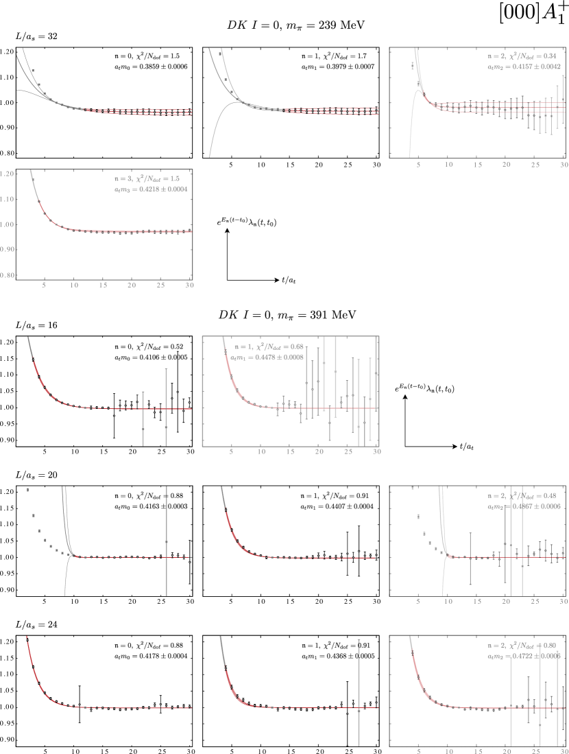
Figure 20: The principal correlators, plotted as $e^{E_{\mathfrak{n}}(t-t_{0})}\lambda_{\mathfrak{n}}(t,t_{0})$, obtained for $DK$ $I=0$ in the $[000]A_{1}^{+}$ irrep with $m_{\pi}=239$ MeV (top) and $m_{\pi}=391$ MeV (bottom). Points shown in grey were not included in the fit. The red curves show the result of two-exponential fits as detailed in Section 2 (this fit form enforces $\lambda_{\mathfrak{n}}(t_{0},t_{0})=1$). The mass extracted from the leading exponential and the $\chi^{2}/N_{\mathrm{dof}}$ are indicated for each fit. These principal correlators correspond to the levels shown in Figs. 3 and 4; faded plots correspond to levels shown in grey in those figures and these are not used in the scattering analyses.

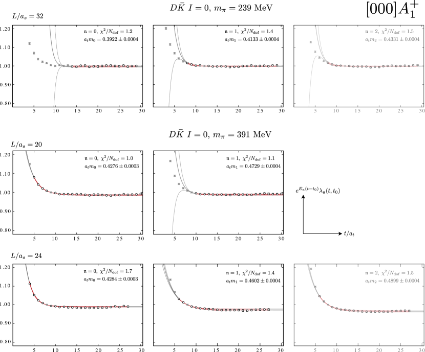
Figure 21: As Fig. 20 but for $D\bar{K}$ $I=0$. These correspond to levels shown in Figs. 5 and 6.

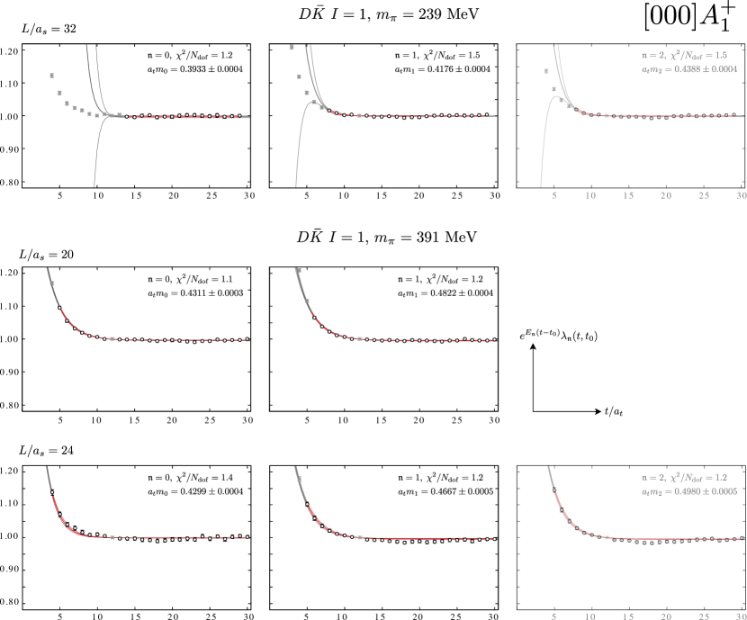
Figure 22: As Fig. 20 but for $D\bar{K}$ $I=1$. These correspond to levels shown in Figs. 5 and 7.

Appendix C Covariance-adjusted and uncorrelated $D\bar{K}$ fits

Tables 11, 12, 13 and 14 present details of $D\bar{K}$ $I=0$ and $I=1$ scattering amplitude fits discussed in Sections 5.2 and 5.3.

	$r=0.001$	$r=0.002$	$r=0.005$	$r=0.01$	uncorr.
$a_{0}/a_{t}$	$9.4\pm 2.0$	$9.5\pm 2.4$	$8.9\pm 2.9$	$8.3\pm 3.4$	$5.3\pm 2.4$
$r_{0}/a_{t}$	$32\pm 12$	$33\pm 14$	$31\pm 18$	$26\pm 24$	$-9\pm 55$
$a_{1}/a_{t}$	$-65\pm 95$	$-62\pm 108$	$-100\pm 140$	$-114\pm 240$	$-240\pm 220$
$a_{2}/a_{t}$	$-15100\pm 8700$	$-17200\pm 10500$	$-20500\pm 14500$	$-23000\pm 18000$	$-36000\pm 32000$
corr.	$\left[\begin{smallmatrix}&1&0.93&0.57&0.53\\ &&1&0.30&0.36\\ &&&1&0.68\\ &&&&1\end{smallmatrix}\right]$	$\left[\begin{smallmatrix}&1&0.94&0.63&0.61\\ &&1&0.40&0.45\\ &&&1&0.67\\ &&&&1\end{smallmatrix}\right]$	$\left[\begin{smallmatrix}&1&0.95&0.69&0.65\\ &&1&0.54&0.55\\ &&&1&0.61\\ &&&&1\end{smallmatrix}\right]$	$\left[\begin{smallmatrix}&1&0.96&0.74&0.67\\ &&1&0.63&0.61\\ &&&1&0.55\\ &&&&1\end{smallmatrix}\right]$	$\left[\begin{smallmatrix}&1&0.97&-0.10&0.01\\ &&1&-0.08&0.06\\ &&&1&-0.30\\ &&&&1\end{smallmatrix}\right]$
$N_{\text{adj}}$	3	7	10	12	–
$\chi^{2}/N_{\mathrm{dof}}$	$\frac{11.2}{18-4}=0.80$	$\frac{10.3}{18-4}=0.73$	$\frac{7.46}{18-4}=0.53$	$\frac{5.75}{18-4}=0.41$	$\frac{1.51}{18-4}=0.11$

Table 11: $D\bar{K}$ $I=0$ scattering amplitude fits on the $m_{\pi}=239$ MeV ensemble, as in Eq. 13 but with small eigenvalues adjusted as described in the text (four columns labelled by $r$) or correlations between finite-volume energies set to zero (final column). $N_{\text{adj}}$ is the number of small eigenvalues adjusted. While adjusting the eigenvalues of the covariance matrix could be considered to have reduced the number of degrees of freedom, here the $\chi^{2}/N_{\mathrm{dof}}$ are presented with the original $N_{\mathrm{dof}}$.

	$r=0.002$	$r=0.005$	$r=0.01$	uncorr.
$a_{0}/a_{t}$	$16.1\pm 2.3$	$15.9\pm 2.4$	$16.0\pm 2.5$	$18.3\pm 2.2$
$r_{0}/a_{t}$	$36.4\pm 1.8$	$36.6\pm 1.8$	$36.7\pm 1.8$	$37.3\pm 3.4$
$a_{1}/a_{t}$	$133\pm 27$	$129\pm 29$	$128\pm 30$	$160\pm 39$
$a_{2}/a_{t}$	$4600\pm 1300$	$4400\pm 1400$	$4400\pm 1400$	$4600\pm 1400$
corr.	$\left[\begin{smallmatrix}&1&0.36&0.75&0.75\\ &&1&-0.14&-0.14\\ &&&1&0.91\\ &&&&1\end{smallmatrix}\right]$	$\left[\begin{smallmatrix}&1&0.39&0.74&0.75\\ &&1&-0.12&-0.11\\ &&&1&0.97\\ &&&&1\end{smallmatrix}\right]$	$\left[\begin{smallmatrix}&1&0.37&0.75&0.76\\ &&1&-0.13&-0.13\\ &&&1&0.94\\ &&&&1\end{smallmatrix}\right]$	$\left[\begin{smallmatrix}&1&0.64&-0.06&-0.01\\ &&1&0.05&0.04\\ &&&1&-0.04\\ &&&&1\end{smallmatrix}\right]$
$N_{\text{adj}}$	2	5	7	–
$\chi^{2}/N_{\mathrm{dof}}$	$\frac{18.6}{29-4}=0.74$	$\frac{16.6}{29-4}=0.66$	$\frac{15.6}{29-4}=0.62$	$\frac{29.7}{29-4}=1.19$

Table 12: As Table 11 but for $D\bar{K}$ $I=0$ on the $m_{\pi}=391$ MeV ensembles, Eq. 14.

	$r=0.001$	$r=0.002$	$r=0.005$	uncorr.
$a_{0}/a_{t}$	$-4.61\pm 0.24$	$-4.68\pm 0.27$	$-4.73\pm 0.34$	$-6.21\pm 0.65$
$a_{1}/a_{t}$	$-227\pm 70$	$234\pm 75$	$-226\pm 88$	$-530\pm 190$
$a_{2}/a_{t}$	$-18700\pm 9300$	$19400\pm 10100$	$-21000\pm 12000$	$-54000\pm 29000$
corr.	$\left[\begin{smallmatrix}&1&0.80&0.63\\ &&1&0.68\\ &&&1\end{smallmatrix}\right]$	$\left[\begin{smallmatrix}&1&0.73&0.58\\ &&1&0.62\\ &&&1\end{smallmatrix}\right]$	$\left[\begin{smallmatrix}&1&0.58&0.49\\ &&1&0.45\\ &&&1\end{smallmatrix}\right]$	$\left[\begin{smallmatrix}&1&-0.15&-0.20\\ &&1&-0.20\\ &&&1\end{smallmatrix}\right]$
$N_{\text{adj}}$	4	7	11	–
$\chi^{2}/N_{\mathrm{dof}}$	$\frac{14.7}{18-3}=0.98$	$\frac{13.5}{18-3}=0.90$	$\frac{10.3}{18-3}=0.68$	$\frac{7.01}{18-3}=0.47$

Table 13: As Table 11 but for $D\bar{K}$ $I=1$ on the $m_{\pi}=239$ MeV ensembles, Eq. 15.

	$r=0.002$	$r=0.005$	$r=0.01$	uncorr.
$a_{0}/a_{t}$	$-4.39\pm 0.38$	$-4.24\pm 0.48$	$-4.02\pm 0.57$	$-2.78\pm 0.56$
$r_{0}/a_{t}$	$16.2\pm 3.7$	$-15.0\pm 4.7$	$-13.1\pm 6.2$	$9\pm 19$
$a_{1}/a_{t}$	$-46\pm 16$	$-44\pm 19$	$-41\pm 22$	$-18\pm 34$
$a_{2}/a_{t}$	$-2710\pm 750$	$-2500\pm 890$	$2330\pm 1020$	$2100\pm 1300$
corr.	$\left[\begin{smallmatrix}&1&0.80&0.66&0.66\\ &&1&0.21&0.21\\ &&&1&0.91\\ &&&&1\end{smallmatrix}\right]$	$\left[\begin{smallmatrix}&1&0.82&0.69&0.70\\ &&1&0.31&0.32\\ &&&1&0.85\\ &&&&1\end{smallmatrix}\right]$	$\left[\begin{smallmatrix}&1&0.85&0.68&0.71\\ &&1&0.38&0.39\\ &&&1&0.79\\ &&&&1\end{smallmatrix}\right]$	$\left[\begin{smallmatrix}&1&0.93&-0.14&-0.05\\ &&1&-0.11&-0.04\\ &&&1&-0.03\\ &&&&1\end{smallmatrix}\right]$
$N_{\text{adj}}$	7	13	17	–
$\chi^{2}/N_{\mathrm{dof}}$	$\frac{20.2}{28-4}=0.84$	$\frac{18.5}{28-4}=0.77$	$\frac{15.2}{28-4}=0.63$	$\frac{29.6}{28-4}=1.23$

Table 14: As Table 11 but for $D\bar{K}$ $I=1$ on the $m_{\pi}=391$ MeV ensembles, Eq. 16.

References

- (1) BaBar collaboration, Observation of a narrow meson decaying to at a mass of 2.32-GeV/c2, Phys. Rev. Lett. 90 (2003) 242001 [hep-ex/0304021].
- (2) S. Godfrey and N. Isgur, Mesons in a Relativized Quark Model with Chromodynamics, Phys. Rev. D 32 (1985) 189.
- (3) H.-X. Chen, W. Chen, X. Liu, Y.-R. Liu and S.-L. Zhu, A review of the open charm and open bottom systems, Rept. Prog. Phys. 80 (2017) 076201 [1609.08928].
- (4) CLEO collaboration, Observation of a narrow resonance of mass 2.46 GeV in the final state, and confirmation of the , AIP Conf. Proc. 698 (2004) 497 [hep-ex/0305017].
- (5) LHCb collaboration, D. Johnson, decays: A new (virtual) laboratory for exotic particle searches at LHCb, CERN LHC Seminar, 2020, https://indico.cern.ch/event/900975/.
- (6) LHCb collaboration, A model-independent study of resonant structure in decays, Phys. Rev. Lett. 125 (2020) 242001 [2009.00025].
- (7) LHCb collaboration, Amplitude analysis of the decay, Phys. Rev. D 102 (2020) 112003 [2009.00026].
- (8) G. Moir, M. Peardon, S. M. Ryan, C. E. Thomas and D. J. Wilson, Coupled-Channel , and Scattering from Lattice QCD, JHEP 10 (2016) 011 [1607.07093].
- (9) Hadron Spectrum collaboration, Excited heavy mesons from lattice QCD, AIP Conf. Proc. 1735 (2016) 030007.
- (10) G. Cheung, Spectroscopy of exotic charm mesons from lattice QCD, Ph.D. thesis, Cambridge U., DAMTP, 2019. 10.17863/CAM.32913.
- (11) L. Liu, K. Orginos, F.-K. Guo, C. Hanhart and U.-G. Meissner, Interactions of charmed mesons with light pseudoscalar mesons from lattice QCD and implications on the nature of the , Phys. Rev. D 87 (2013) 014508 [1208.4535].
- (12) D. Mohler, C. Lang, L. Leskovec, S. Prelovsek and R. Woloshyn, Meson and -Meson-Kaon Scattering from Lattice QCD, Phys. Rev. Lett. 111 (2013) 222001 [1308.3175].
- (13) C. Lang, L. Leskovec, D. Mohler, S. Prelovsek and R. Woloshyn, Ds mesons with DK and D*K scattering near threshold, Phys. Rev. D 90 (2014) 034510 [1403.8103].
- (14) G. S. Bali, S. Collins, A. Cox and A. Schäfer, Masses and decay constants of the and from lattice QCD close to the physical point, Phys. Rev. D 96 (2017) 074501 [1706.01247].
- (15) C. Alexandrou, J. Berlin, J. Finkenrath, T. Leontiou and M. Wagner, Tetraquark interpolating fields in a lattice QCD investigation of the meson, Phys. Rev. D 101 (2020) 034502 [1911.08435].
- (16) R. C. Johnson, Angular Momentum on a Lattice, Phys. Lett. 114B (1982) 147.
- (17) D. C. Moore and G. T. Fleming, Angular momentum on the lattice: The Case of non-zero linear momentum, Phys. Rev. D73 (2006) 014504 [hep-lat/0507018].
- (18) C. Michael, Adjoint Sources in Lattice Gauge Theory, Nucl. Phys. B259 (1985) 58.
- (19) M. Luscher and U. Wolff, How to Calculate the Elastic Scattering Matrix in Two-dimensional Quantum Field Theories by Numerical Simulation, Nucl. Phys. B339 (1990) 222.
- (20) J. J. Dudek, R. G. Edwards, N. Mathur and D. G. Richards, Charmonium excited state spectrum in lattice QCD, Phys. Rev. D77 (2008) 034501 [0707.4162].
- (21) J. J. Dudek, R. G. Edwards, M. J. Peardon, D. G. Richards and C. E. Thomas, Toward the excited meson spectrum of dynamical QCD, Phys. Rev. D82 (2010) 034508 [1004.4930].
- (22) Hadron Spectrum collaboration, Energy dependence of the resonance in elastic scattering from lattice QCD, Phys. Rev. D87 (2013) 034505 [1212.0830].
- (23) D. J. Wilson, R. A. Briceno, J. J. Dudek, R. G. Edwards and C. E. Thomas, Coupled scattering in -wave and the resonance from lattice QCD, Phys. Rev. D92 (2015) 094502 [1507.02599].
- (24) Hadron Spectrum collaboration, Tetraquark operators in lattice QCD and exotic flavour states in the charm sector, JHEP 11 (2017) 033 [1709.01417].
- (25) C. E. Thomas, R. G. Edwards and J. J. Dudek, Helicity operators for mesons in flight on the lattice, Phys. Rev. D85 (2012) 014507 [1107.1930].
- (26) J. J. Dudek, R. G. Edwards and C. E. Thomas, S and D-wave phase shifts in isospin-2 pi pi scattering from lattice QCD, Phys. Rev. D86 (2012) 034031 [1203.6041].
- (27) M. Padmanath, C. Lang and S. Prelovsek, X(3872) and Y(4140) using diquark-antidiquark operators with lattice QCD, Phys. Rev. D 92 (2015) 034501 [1503.03257].
- (28) A. J. Woss, C. E. Thomas, J. J. Dudek, R. G. Edwards and D. J. Wilson, resonance in coupled , scattering from lattice QCD, Phys. Rev. D 100 (2019) 054506 [1904.04136].
- (29) Hadron Spectrum collaboration, A Novel quark-field creation operator construction for hadronic physics in lattice QCD, Phys. Rev. D80 (2009) 054506 [0905.2160].
- (30) R. G. Edwards, B. Joo and H.-W. Lin, Tuning for Three-flavors of Anisotropic Clover Fermions with Stout-link Smearing, Phys. Rev. D78 (2008) 054501 [0803.3960].
- (31) Hadron Spectrum collaboration, First results from 2+1 dynamical quark flavors on an anisotropic lattice: Light-hadron spectroscopy and setting the strange-quark mass, Phys. Rev. D79 (2009) 034502 [0810.3588].
- (32) Hadron Spectrum collaboration, Excited and exotic charmonium spectroscopy from lattice QCD, JHEP 07 (2012) 126 [1204.5425].
- (33) Hadron Spectrum collaboration, Excited and exotic charmonium, and meson spectra for two light quark masses from lattice QCD, JHEP 12 (2016) 089 [1610.01073].
- (34) D. J. Wilson, R. A. Briceno, J. J. Dudek, R. G. Edwards and C. E. Thomas, The quark-mass dependence of elastic scattering from QCD, Phys. Rev. Lett. 123 (2019) 042002 [1904.03188].
- (35) R. G. Edwards, J. J. Dudek, D. G. Richards and S. J. Wallace, Excited state baryon spectroscopy from lattice QCD, Phys. Rev. D84 (2011) 074508 [1104.5152].
- (36) D. J. Wilson, J. J. Dudek, R. G. Edwards and C. E. Thomas, Resonances in coupled scattering from lattice QCD, Phys. Rev. D91 (2015) 054008 [1411.2004].
- (37) Hadron Spectrum collaboration, An resonance in strongly coupled , scattering from lattice QCD, Phys. Rev. D93 (2016) 094506 [1602.05122].
- (38) M. T. Hansen and S. R. Sharpe, Lattice QCD and Three-particle Decays of Resonances, Ann. Rev. Nucl. Part. Sci. 69 (2019) 65 [1901.00483].
- (39) M. Luscher, Volume Dependence of the Energy Spectrum in Massive Quantum Field Theories. 2. Scattering States, Commun. Math. Phys. 105 (1986) 153.
- (40) M. Luscher, Two particle states on a torus and their relation to the scattering matrix, Nucl. Phys. B354 (1991) 531.
- (41) M. Luscher, Signatures of unstable particles in finite volume, Nucl. Phys. B364 (1991) 237.
- (42) K. Rummukainen and S. A. Gottlieb, Resonance scattering phase shifts on a nonrest frame lattice, Nucl. Phys. B450 (1995) 397 [hep-lat/9503028].
- (43) C. h. Kim, C. T. Sachrajda and S. R. Sharpe, Finite-volume effects for two-hadron states in moving frames, Nucl. Phys. B727 (2005) 218 [hep-lat/0507006].
- (44) N. H. Christ, C. Kim and T. Yamazaki, Finite volume corrections to the two-particle decay of states with non-zero momentum, Phys. Rev. D72 (2005) 114506 [hep-lat/0507009].
- (45) Z. Fu, Rummukainen-Gottlieb’s formula on two-particle system with different mass, Phys. Rev. D85 (2012) 014506 [1110.0319].
- (46) L. Leskovec and S. Prelovsek, Scattering phase shifts for two particles of different mass and non-zero total momentum in lattice QCD, Phys. Rev. D85 (2012) 114507 [1202.2145].
- (47) R. A. Briceno, Two-particle multichannel systems in a finite volume with arbitrary spin, Phys. Rev. D 89 (2014) 074507 [1401.3312].
- (48) R. A. Briceno, J. J. Dudek and R. D. Young, Scattering processes and resonances from lattice QCD, Rev. Mod. Phys. 90 (2018) 025001 [1706.06223].
- (49) G. F. Chew and S. Mandelstam, Theory of low-energy pion pion interactions, Phys. Rev. 119 (1960) 467.
- (50) G. Moir, M. Peardon, S. M. Ryan, C. E. Thomas and L. Liu, Excited spectroscopy of charmed mesons from lattice QCD, JHEP 05 (2013) 021 [1301.7670].
- (51) Particle Data Group collaboration, Review of Particle Physics, Phys. Rev. D 98 (2018) 030001.
- (52) S. Weinberg, Evidence That the Deuteron Is Not an Elementary Particle, Phys. Rev. 137 (1965) B672.
- (53) A. Martínez Torres, E. Oset, S. Prelovsek and A. Ramos, Reanalysis of lattice QCD spectra leading to the and , JHEP 05 (2015) 153 [1412.1706].
- (54) Z.-H. Guo, L. Liu, U.-G. Meißner, J. Oller and A. Rusetsky, Towards a precise determination of the scattering amplitudes of the charmed and light-flavor pseudoscalar mesons, Eur. Phys. J. C 79 (2019) 13 [1811.05585].
- (55) A. Sitenko, Lectures in Scattering Theory. Pergamon Press, Oxford, 1971.
- (56) J. R. Taylor, Scattering Theory: The Quantum Theory of Nonrelativistic Collisions. Dover, Mineola, NY, 2006.
- (57) T. Iritani, S. Aoki, T. Doi, T. Hatsuda, Y. Ikeda, T. Inoue et al., Are two nucleons bound in lattice QCD for heavy quark masses? Consistency check with Lüscher’s finite volume formula, Phys. Rev. D 96 (2017) 034521 [1703.07210].
- (58) M. Albaladejo, P. Fernandez-Soler, F.-K. Guo and J. Nieves, Two-pole structure of the , Phys. Lett. B 767 (2017) 465 [1610.06727].
- (59) M.-L. Du, M. Albaladejo, P. Fernández-Soler, F.-K. Guo, C. Hanhart, U.-G. Meißner et al., Towards a new paradigm for heavy-light meson spectroscopy, Phys. Rev. D 98 (2018) 094018 [1712.07957].
- (60) A. Francis, R. J. Hudspith, R. Lewis and K. Maltman, Lattice Prediction for Deeply Bound Doubly Heavy Tetraquarks, Phys. Rev. Lett. 118 (2017) 142001 [1607.05214].
- (61) A. Francis, R. J. Hudspith, R. Lewis and K. Maltman, Evidence for charm-bottom tetraquarks and the mass dependence of heavy-light tetraquark states from lattice QCD, Phys. Rev. D 99 (2019) 054505 [1810.10550].
- (62) P. Junnarkar, N. Mathur and M. Padmanath, Study of doubly heavy tetraquarks in Lattice QCD, Phys. Rev. D 99 (2019) 034507 [1810.12285].
- (63) L. Leskovec, S. Meinel, M. Pflaumer and M. Wagner, Lattice QCD investigation of a doubly-bottom tetraquark with quantum numbers , Phys. Rev. D 100 (2019) 014503 [1904.04197].
- (64) T. A. Kaeding, Tables of SU(3) isoscalar factors, Atom. Data Nucl. Data Tabl. 61 (1995) 233 [nucl-th/9502037].
- (65) U.-G. Meißner, Two-pole structures in QCD: Facts, not fantasy!, Symmetry 12 (2020) 981 [2005.06909].
- (66) SciDAC, LHPC, UKQCD collaboration, The Chroma software system for lattice QCD, Nucl. Phys. Proc. Suppl. 140 (2005) 832 [hep-lat/0409003].
- (67) M. A. Clark, R. Babich, K. Barros, R. C. Brower and C. Rebbi, Solving Lattice QCD systems of equations using mixed precision solvers on GPUs, Comput. Phys. Commun. 181 (2010) 1517 [0911.3191].
- (68) R. Babich, M. A. Clark and B. Joo, Parallelizing the QUDA Library for Multi-GPU Calculations in Lattice Quantum Chromodynamics, in SC 10 (Supercomputing 2010) New Orleans, Louisiana, November 13-19, 2010, 2010, http://www1.jlab.org/Ul/publications/view_pub.cfm?pub_id=10186 [1011.0024].
- (69) B. Joó, D. D. Kalamkar, K. Vaidyanathan, M. Smelyanskiy, K. Pamnany, V. W. Lee et al., Lattice QCD on Intel® Xeon Phi Coprocessors, Lect. Notes Comput. Sci. 7905 (2013) 40.
- (70) J. C. Osborn, R. Babich, J. Brannick, R. C. Brower, M. A. Clark, S. D. Cohen et al., Multigrid solver for clover fermions, PoS LATTICE2010 (2010) 037 [1011.2775].
- (71) R. Babich, J. Brannick, R. C. Brower, M. A. Clark, T. A. Manteuffel, S. F. McCormick et al., Adaptive multigrid algorithm for the lattice Wilson-Dirac operator, Phys. Rev. Lett. 105 (2010) 201602 [1005.3043].