Spots and flares in hot main sequence stars

Abstract

About 22000 Kepler stars and nearly 60000 TESS stars from sectors 1–24 have been classified according to variability type. A large proportion of stars of all spectral types appear to have periods consistent with the expected rotation periods. A previous analysis of A and late B stars strongly suggests that these stars are indeed rotational variables. In this paper we have accumulated sufficient data to show that rotational modulation is present even among the early B stars. A search for flares in TESS A and B stars resulted in the detection of 110 flares in 68 stars. The flare energies exceed those of typical K and M dwarfs by at least two orders of magnitude. These results, together with severe difficulties of current models to explain stellar pulsations in A and B stars, suggest a need for revision of our current understanding of the outer layers of stars with radiative envelopes.

1 Introduction

High-precision space photometry of upper main sequence stars show periodic or quasi-periodic variations with periods consistent with the expected rotational periods of these stars (Balona, 2013, 2016, 2017, 2019). High-resolution spectroscopic time series of Vega (A0V) indicates the presence of a spotted stellar surface(Böhm et al., 2015), providing independent confirmation of the photometric results.

In addition, early results from the Kepler mission (Borucki et al., 2010) indicated the presence of flares associated with some A and late-B stars (Balona, 2012). Further studies (Balona, 2013, 2015; Balona et al., 2016b) seem to indicate that around 2.5 percent of A stars flare with energies in the range $10^{35}$–$10^{36}$ erg. Pedersen et al. (2017) have argued that the flares are likely a result of cool flare stars in the same aperture or binary companions. Direct evidence of possible X-ray flares in A stars have been reported by Schmitt et al. (1994), Robrade & Schmitt (2010), while a flare on a B star has also been reported (Yanagida et al., 2004; Yanagida et al., 2007).

Rotational modulation and flares in A and B stars implies the presence of surface magnetic fields, contrary to the long-held view that it is not possible for stars with radiative envelopes to host magnetic fields. The Ap and Bp stars have strong global magnetic fields, but these are explained as being of fossil origin (Mestel, 1967). Photometric studies referenced above indicate that rotational modulation is present in as many as 40 percent of stars on the upper main sequence, most of which are not known Ap/Bp stars.

First results from the Kepler space mission on pulsations in main-sequence A stars (Grigahcène et al., 2010) already indicated a serious problem. It turns out that nearly all $\delta$ Scuti stars have multiple low frequency pulsations which cannot be explained by current models (Balona, 2014, 2018). A further surprise was the confirmation that many late-B stars pulsate with high frequencies (Maia variables, Balona et al. 2015; Balona et al. 2016a; Balona & Ozuyar 2020b). These are difficult to explain in terms of incorrect opacities alone (Daszyńska-Daszkiewicz et al., 2017). Perhaps of even more significance is the fact that less than half of the stars in the $\delta$ Sct instability strip pulsate. Also it seems that the $\gamma$ Dor variables may be just a subset of the $\delta$ Sct stars (Balona, 2018). None of these findings are explained by current pulsation models.

New ideas regarding the outer layers of stars in radiative envelopes have recently emerged. It has been suggested, for example, that generation of magnetic fields by dynamo action may occur in sub-surface convective zones in A and B stars (Cantiello et al., 2009; Cantiello & Braithwaite, 2011, 2019). At the surface they give rise to bright starspots. Also, it has been suggested that differential rotation may act to provide dynamo-generated magnetic fields in radiative zones (Spruit, 1999, 2002; Maeder & Meynet, 2004).

In this paper we report on further evidence for rotational modulation among TESS A and B stars, indicating that starspots are common among all B stars, including the early-type B stars. We also report on a survey for flares in TESS stars on the upper main sequence. We argue that current ideas regarding the outer layers of stars in radiative equilibrium need to be revised.

2 Data and methodology

The data used here are the full four-year light curves from Kepler and sectors 1–24 of TESS data. In both cases the light curves are obtained using pre-search data conditioning (PDC) which corrects for time-correlated instrumental signatures in the light curves (Jenkins et al., 2016). All stars with effective temperatures $T_{\rm eff}>6000$ K brighter than magnitude 12.5 were selected for the analysis of rotational modulation. This results in 5643 stars from Kepler and over 50000 stars from TESS. In the search for flares, the uncorrected light curves were used and only stars with $T_{\rm eff}>7500$ K were selected.

Visual inspection of the light curves and the Lomb-Scargle periodograms (Scargle, 1982) of Kepler and TESS stars were used to assign variability types whenever appropriate. The variability classification follows that of the General Catalogue of Variable Stars (GCVS, Samus et al. 2017). The only recognized class of rotational variable among the A and B stars are the chemically peculiar $\alpha$ CVn and SX Ari classes. A new ROT class has been added to describe any star in which the variability is suspected to be due to rotation and not known to be Ap or Bp. Aided by suitable software, visual classification of over 100 stars an hour is possible. In this way, several thousand stars with $T_{\rm eff}>6000$ K have been assigned the ROT type.

3 Stellar parameters

The most commonly used test for rotational modulation is comparison of the rotation rate derived from the photometric frequency, $\nu_{\rm ROT}$, with that derived from the projected rotational velocity, $v\sin i$. To derive the equatorial rotational velocity, $v$, from $\nu_{\rm ROT}$ requires an estimate of the stellar radius, $R$. This can be done if we know the effective temperature, $T_{\rm eff}$ and luminosity, $L/L_{\odot}$.

The most precise method of deriving $T_{\rm eff}$ is by modelling absorption line profiles from medium- or high-resolution spectroscopy. For A and B stars, this involves fitting the H$\beta$ and/or H$\alpha$ line profiles using a suitable model atmosphere. The resulting standard deviation in $T_{\rm eff}$ ranges from about 100 K for A stars to about 1000 K for early B stars. Spectroscopic estimates of $T_{\rm eff}$ exist for about 25 percent of the sample considered here.

The next best method is the use of narrow-band photometry. This involves measuring the strength of the H$\beta$ line (the Strömgren $\beta$ index) usually in conjunction with $uvby$ narrow-band photometry. The value of $T_{\rm eff}$ is obtained either by direct comparison with synthetic photometry derived from model atmospheres or by using stars with known $T_{\rm eff}$ (Moon & Dworetsky, 1985; Gray, 1991; Napiwotzki et al., 1993; Smalley & Dworetsky, 1993; Balona, 1994). Estimates of $T_{\rm eff}$ from Sloan $ugriz$ (Brown et al., 2011) are of this type and are available for most of the Kepler and TESS stars. However, they cannot be used for stars earlier than A0 because they lack $u$-band measurements. Without the $u$ band, it is impossible to distinguish between A and B stars of the same colour. Estimates of $T_{\rm eff}$ using narrow- and intermediate-band photometry are available for about 55 percent of stars.

If neither spectroscopy or narrow-band photometry is available, wide-band photometry can be used to estimate $T_{\rm eff}$ provided that the reddening is known. This method is used in 7 percent of our sample. Finally, if nothing else is available, a crude estimate of $T_{\rm eff}$ can be derived from the spectral classification together with suitable calibration such as the calibration of Pecaut & Mamajek (2013). This method was used for 18 percent of the stars.

The stellar luminosity is best estimated from Gaia DR2 parallaxes (Gaia Collaboration et al., 2016; Gaia Collaboration et al., 2018) in conjunction with reddening estimated using a three-dimensional map by Gontcharov (2017) and the bolometric correction calibration by Pecaut & Mamajek (2013). From the error in the Gaia DR2 parallax, the typical standard deviation in $\log(L/L_{\odot})$ is estimated to be about 0.05 dex, allowing for standard deviations of 0.01 mag in the apparent magnitude, 0.10 mag in visual extinction and 0.02 mag in the bolometric correction in addition to the parallax error.

Table 1: Number of ROT stars within the given $T_{\rm eff}$ range, $N_{\rm ROT}$. Also shown is the fraction of ROT stars, $f_{\rm ROT}$ within the range. $N_{\rm vsini}$ is the number of stars used to construct the $v\sin i$ vs $v$ diagrams (Fig. 1 left panel) and $N_{\rm dist}$ is the number of stars used in obtaining the $v\sin i$ distribution (Fig. 1 right panel).

$T_{\rm eff}$	$N_{\rm ROT}$	$f_{\rm ROT}$	$N_{\rm vsini}$	$N_{\rm dist}$
6000–7000	21835	0.50	3329	7128
7000–8000	3298	0.34	239	1459
8000–10000	2418	0.31	420	2068
10000–12000	529	0.40	205	866
12000–18000	341	0.37	219	1417
18000–30000	138	0.29	85	1481

Table 1 lists the number of stars classified as ROT variables in the given range of effective temperature. Also shown is the percentage of main sequence stars for which the ROT classification was assigned. Note that Be stars were excluded from the sample. While the light variations in Be stars can be interpreted as rotational modulation, the light amplitude is typically an order of magnitude larger than for non-Be stars (Balona & Ozuyar, 2020a). It is suggested that the cause of the variability are co-rotating clouds which obscure a larger fraction of the photosphere than starspots. Because of the large amplitude, Be stars are disproportionately represented among the ROT stars. Since Be stars are rapid rotators, their inclusion leads to an over-estimate of the proportion of ROT stars with rapid rotation. Most Be stars are of early B type and this leads to a severe distortion of the velocity distribution for stars with $T_{\rm eff}>18000$ K.

4 Results

The photometric period, obtained from Kepler, K2 and TESS light curves together with the stellar radius is used to estimate the equatorial rotational velocity, $v$. If the variability is rotational modulation, there should be a relationship between $v$ and the projected rotational velocity, $v\sin\,i$. Since most stars will be observed roughly equator-on, one expects that most data points in the $v$–$v\sin i$ diagram will lie on or just below the straight line defining $\sin i=1$. There will be a diminishing scatter of points below the line due to stars with lower angles of inclination, $i$. Due to unavoidable errors, some points are to be expected above the $v\sin i=1$ line.

Projected rotational velocities are not available for every star for which $v$ has been estimated. In the left panel of Fig. 1, the $v$–$v\sin i$ diagram is shown for all stars for which measurements are available. It is clear that the expected distribution of points is present from the F stars to the early B stars. This justifies the original assumption that the periodic light variation is due to rotation.

As expected, nearly all stars with $v>60$ km s^-1 lie on or below the $\sin i=1$ line. For low rotation rates, ever increasing observational precision is required to determine whether or not $v\sin i<v$. Often, $v\sin i$ values are truncated at some positive number corresponding to the resolution limit of the instrument. An important factor is that it becomes increasingly difficult to distinguish between binarity and rotation at low frequencies. For example, amplitude variability, which is a typical attribute of rotational modulation, is not so easily detected. Thus one may expect significant contamination from binaries at low rotation rates. These factors are probably responsible for the increased scatter in this region.

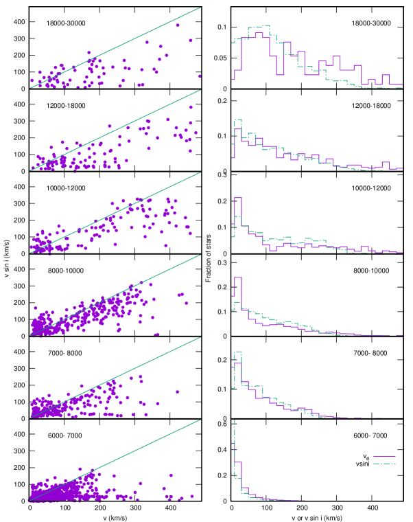
Figure 1: Left panel: the relationship between the projected rotational velocity, $v\sin i$ and the equatorial rotational velocity, $v$ (estimated from the photometric frequency), for different ranges of $T_{\rm eff}$ (labeled). The straight line corresponds to $v=v\sin i$. Right panel: the distribution of equatorial rotational velocity (solid violet) and $v\sin i$ (dashed blue) for different ranges of $T_{\rm eff}$. In both cases Be stars are omitted.

A more rigorous test can be made by considering the rotational velocity distribution for main-sequence stars within a limited $T_{\rm eff}$ range. The rotational velocity distribution is the relative number of stars at a given rotational velocity. This is an important quantity which provides information on the physics of stellar rotation. The test involves the comparison of the $v$ distribution with the $v\sin i$ distribution. These two distributions should be similar, though not identical due to variation of the inclination of the rotation axis. Close agreement is expected because most stars would be viewed equator-on. This is a far more rigorous test because it involves not just comparison of $v$ and $v\sin i$ for the same star, but also tests whether the detailed distribution of $v$ corresponds closely to that of $v\sin i$.

It might be thought that one could derive $v$ from $v\sin i$ by deconvolution assuming random orientation of the axis of rotation. In this way one could compare the photometric and spectroscopic $v$ directly. The reason why this has not been done is that the stars from which the photometric $v$ are derived cannot have a random axis of rotation. Clearly, if a star is nearly pole-on, no rotational modulation will be detected. This is, of course, not true for $v\sin i$ since rotational broadening can be made for any inclination angle. Therefore the distribution of $v$ from deconvolution of $v\sin i$ cannot match the photometric $v$ distribution. For the same reason, testing the distribution of $i$ is not possible.

Obtaining the distribution requires sufficient numbers of stars within the chosen range of $v$ or $v\sin i$ in order to be statistically meaningful. The number of stars for which photometric $v$ measurements are available is sufficiently large for this purpose. If the corresponding values of $v\sin i$ are restricted to the same stars for which $v$ is available, the numbers would be too small. Fortunately, it is not necessary to impose this restriction because it is reasonable to assume that the $v\sin i$ distribution will be the same for any set of main-sequence stars within the chosen range of $T_{\rm eff}$. In other words, one may select any set of main sequence stars with known $v\sin i$ within the required effective temperature range.

In the right panel of Fig. 1, the $v$ and $v\sin i$ distributions for stars in six temperature ranges are shown. There is good agreement for all temperature ranges, reinforcing the results derived from the $v$–$v\sin i$ diagrams.

5 TESS early-type flare stars

In our catalog of nearly 60000 stars classified for variability, there are 14495 stars with $T_{\rm eff}>7500$ K. Flares are difficult to detect in eclipsing binaries and other types of variable with high amplitude. Excluding these stars results in 6072 A and 1616 B stars. This sample was searched for flares by visual inspection.

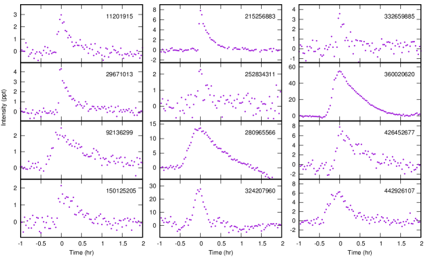
Figure 2: Examples of A star flares in the TESS data. The time origin is the time of maximum flare intensity. Time is in hours and intensity if parts per thousand.

The 68 stars in Table 2 appear to have flare-like events, examples of which are shown in Fig. 2. A substantial proportion of the flare stars are X-ray sources. Multiple flares are visible in 23 stars, giving a total of 110 flare events. Not included here are the TESS A-type flare stars TIC 118327563 and TIC 224244458 (Balona et al., 2019a). The former is a sdB star and the latter is an SX Ari variable (Bp star). Also excluded is the $\delta$ Sct flare star TIC 439399707 (Balona et al., 2019b) and the Be X-ray source TIC 207176480 (Balona & Ozuyar, 2020a).

The number of TESS A-type stars which appear to flare constitute about 1.1 percent of the sample of A stars which were examined, which is less than half of the 2.5 percent flare incidence among Kepler A stars reported by Balona (2013) and Balona (2015). This can be understood given the fact that the long-cadence Kepler data span 4 years, while the TESS data mostly span a few months and always less than one year. There are 61 Kepler A stars known to flare (Balona, 2015). The additional 68 flare stars reported here do not include any of the Kepler stars, bringing the total of flaring A stars to 129.

Whereas the Kepler pixel size is 4 arcsec, the TESS pixel size is 21 arcsec. This means that the probability of a flare originating in a star other than the A star is much larger for TESS. The fields of all 68 stars were examined and in each case the A star is by far the dominant optical source. Any cool star in the aperture would need to be of comparable brightness to the A star for the flare to be detected. A cool dwarf within the same aperture would be among the nearest stars and would have long ago been catalogued. Therefore the source of the flare would need to be an exotic faint object, a companion of the A star or the A star itself.

The flare energy was estimated by integrating the light curve under the flare. In cool dwarfs and the Sun, most of the flare energy is radiated in the UV. The UV contribution in Kepler and TESS light curves is negligible, and therefore the estimated flare energy is likely to be an underestimate. As can be seen from Table 2, the typical flare energy is $10^{35}$–$10^{36}$ erg, which is about 10-1000 times more energetic than flares in cool dwarfs. The most energetic flare in cool dwarfs detected in a survey of TESS stars by Maximilian et al. (2020) has an energy of $10^{34.7}$ erg. It is difficult to understand how a unique event like this can be repeated in over 1 percent of A stars. Multiple flares in the same star, all with energies exceeding the highest ever seen, also would seem to rule out a cool companion.

Table 2: Flare stars detected from visual inspection of TESS light curves. The TIC and HD numbers are followed by the assigned variability class. This is followed by the effective temperature (K) and luminosity. The time of peak flare intensity, $t_{\rm max}$, is relative to BJD 2458000. The flare energy, $E$ (erg), is followed by the relative peak flare intensity, $\tfrac{\Delta F}{F}$. The number of flares, $N_{\rm Fl}$, is followed by a reference to X-ray detection and the spectral type.

TIC	HD	Type	$T_{\rm eff}$	$\log L/L_{\odot}$	$t_{\rm max}$	$\log E$	$\log\tfrac{\Delta F}{F}$	$N_{\rm Fl}$	Ref.	Sp.Type
11201915	37410		7966	1.26	486.73	35.3	-2.528	1	1	kA4hA2VmA7
11895653	103287		9650	1.80	909.93	36.1	-2.783	3	2	A0Ve+K2V SB
22562087	107143	ROT	8234	1.20	588.46	35.3	-2.457	1		A1V
25424318	111608	ROT	9155	1.40	573.68	35.9	-1.972	1		A1IV
26893151	11060	ROT	8494	1.18	780.81	36.3	-2.196	2	3	A0
28643592	174830	ROT	7953	1.63	689.40	35.6	-2.476	1		A2
29671013	200052		8892	1.47	336.79	35.7	-2.367	1		A5V:pSiMg
30052567	76516	ROT	8971	1.42	538.25	36.3	-2.067	1		A0V
34404183	152384	ROT	9096	1.55	648.00	36.4	-2.552	1		A0V
50624799	36118	ROT	11183	1.80	489.77	36.7	-2.012	1	4	B9V
55219038	43620	ROT	8476	1.43	862.38	35.5	-2.534	1		A2
75873633	133574	ROT	7078	0.92	618.67	35.6	-2.128	2		A9/F0V
92136299	222661	ROT	10618	1.73	380.64	36.2	-2.607	3	5	B9.5IV
94336006	24300		13520	2.35	794.21	36.7	-2.453	1		B8III?
125958765	154426	ROT	7915	1.24	649.17	36.1	-1.984	1	3	A7III
142268253	16754	ROT	8997	1.40	397.15	35.4	-2.915	2	2	A1Va
142457761	90759		8778	1.12	709.40	35.7	-2.231	2		A2
147622676	94660	ACV	9544	1.77	575.02	36.1	-2.559	1	3	A0pEuCrSi(Sr)
150125205	29646	ROT	9594	1.76	819.61	35.7	-2.671	1	3	A1IV
150250959	44532	ROT	8072	1.21	451.68	35.8	-2.073	1		A2V
160644410	131461	ROT	8396	1.52	615.16	36.4	-1.705	1	3	A0/1V
177284702	51581		7266	0.56	661.79	35.5	-1.722	1		A8V
199752613	35885	ROT	9566	1.09	472.60	37.0	-1.332	2		A0
215256883	17864	ROT	9542	1.48	400.63	36.0	-2.107	2	3	B9.5V
220399820	29578	ACV	7415	1.40	394.36	35.7	-2.312	1		A4SrEuCr
233164000	108346	ROT	9522	1.42	916.76	35.6	-2.548	1		kA1hA9mF2
236003103	195984	ROT	9900	1.50	821.51	36.0	-2.317	2		A0V
248430494	33190	ROT	15100	2.17	447.91	36.5	-2.499	1		B8V
248992635	33819		8735	1.26	453.52	35.8	-2.164	1		A0V
252834311	20842	ROT	9900	1.39	804.06	35.4	-2.643	1		A0Va+
256749693	191174	ROT	9170	1.40	699.39	35.7	-2.325	1	2	A2II-III
260416268	45229		7537	1.29	336.89	35.8	-2.291	2	2	kA2hA7VmA7
264593064	35134	ROT	8193	1.49	487.26	35.6	-2.658	6	3	A2V
264683456	36030	ROT	8992	1.70	488.89	36.6	-2.123	1	6	A0
269833435	196816		8129	1.02	329.45	35.0	-2.722	1		A3/5III
280965566	83719	ROT	7992	1.81	559.25	37.0	-1.866	1	3	A0V
284084463	22961	ACV	9650	1.37	810.20	36.2	-2.100	1		A1pSr
287178418	86001	ROT	7749	1.13	856.61	35.9	-2.049	1		A2V
287329624	57642	ROT	6900	0.84	478.19	35.2	-2.380	1		A8IV/V
299899924	54682	ROT	7404	1.50	488.61	36.4	-2.044	4		A0V
301749125	155056	ROT	9241	1.39	664.92	35.8	-2.247	2		A2V
313942295	170868	ROT	10809	2.88	656.15	38.5	-1.601	1	7	B8/A1
324207960	169484	ROT	7175	1.84	656.45	36.9	-1.558	1	3	A8/9III/IV
324892747	173842		7555	1.33	664.99	36.8	-1.974	1		A7IV
327136878	9622	ROT	5978	0.64	814.03	34.8	-2.341	1		A0pSi?
327724630	209468	ROT	8906	1.48	341.54	35.5	-2.619	1		A1V
332659885	26624	ROT	7960	1.14	452.09	35.2	-2.447	2		A2/3V
337220792	20769	ROT	9631	1.35	423.21	36.0	-2.161	1		A0V
349193923	56911	ROT	9624	1.47	521.06	36.0	-2.310	2		A0Vs
352939640	25553	ROT	9900	1.43	827.25	35.7	-2.430	2		A0V
357633579	79490	ROT	8063	1.18	552.43	36.3	-2.207	2	3	A1/2V
358467237	NGC2516 4	ROT	6379	0.95	333.98	36.3	-1.815	2	8	A7III
360020620	190833	ROT	9900	1.28	700.05	37.0	-1.261	10	3	A0V
393389739	43881	ROT	9123	1.32	493.71	36.0	-2.642	1		A2V
395007683	97049	ROT	9034	1.19	646.65	35.4	-2.209	1		A2V
404477098	15527	ROT	6929	1.22	423.25	37.0	-1.343	1		A9V
407825808	163837	ROT	7023	0.83	627.18	35.5	-2.103	1	9	A9V
409135458	56832	ROT	7495	1.53	492.11	36.7	-2.164	1		A1II/III
426452677	143474	ROT	7620	1.29	636.71	36.0	-2.109	1	2	A5IVs
427393202	294262	ROT	6962	1.71	478.46	36.8	-2.057	1	3	A0
427458366	290674	ROT	8416	1.53	481.88	35.9	-2.347	1		A0V
434109154	GD 1214		8680	1.81	369.38	38.2	-0.793	1
438598966	116649	ROT	8200	1.22	608.60	35.8	-2.506	1		A0V
440863421	131885	ROT	8793	1.47	616.47	35.3	-2.882	2		A0V
442926107	35308	ROT	8631	1.42	455.54	36.2	-2.431	2		A0V
443316662	45341	ROT	7159	1.13	474.24	35.7	-2.591	2		A2
452468734	80950	ROT	10069	1.61	592.16	35.2	-2.776	1		A0V
459786991	82861	ROT	7537	1.29	870.87	35.9	-2.510	5	3	kA2mF0
References:
1- Lo et al. (2014); 2 - Schröder & Schmitt (2007); 3 - Voges et al. (1999); 4 - Evans et al. (2013); 5 - Makarov (2003);
6 - Evans et al. (2019); 7 - Berghoefer et al. (1996); 8 - Marino et al. (2006); 9 - Voges et al. (2000)

6 Conclusion

It is demonstrated that the periodic light variations seen in about 40 percent of A and B stars is consistent with rotational modulation. The expected relationship between the estimated equatorial rotation velocity, $v$, and the projected rotation velocity, $v\sin i$, is confirmed for B stars in three effective temperature ranges. Furthermore, the detailed distribution of $v$ matches the distribution of $v\sin i$ even for the hottest B stars.

Balona & Ozuyar (2020a) proposed a model for Be stars in which the energy released by flares and magnetic reconnection, in conjunction with rapid rotation, ejects gas which is trapped in two diametrically opposite locations defined by the intersection of the geographic and magnetic equators. This gas eventually dissipates into the circumstellar disc. This model appears to explain most of the known characteristics of Be stars.

In this analysis Be were excluded, even though they appear to show rotational modulation (Balona & Ozuyar, 2020a). It turns out that the rotational light amplitudes are an order of magnitude larger than in non-Be stars. Rotational modulation in Be stars is, after all, detectable from the ground which is not true of most A and B stars. The large amplitude in Be stars may possibly be a result of circumstellar clouds rather than starspots (Balona & Ozuyar, 2020a). Due to their rapid rotation, inclusion of Be stars will distort the true velocity distribution. A full discussion of activity and rotation in Be stars will be presented elsewhere.

The nature of the presumed starspots responsible for rotational modulation is not known. The idea of magnetic field generation in subsurface convective zones first postulated by Cantiello et al. (2009); Cantiello & Braithwaite (2011); Cantiello et al. (2011); Cantiello & Braithwaite (2019) seems to be quite promising. However, one would have expected that starspots should occur only within certain effective temperature ranges depending on the ionization species.

According to Cantiello & Braithwaite (2019), the largest effects are caused by a convective layer driven by second helium ionization. The amplitude of surface magnetic fields and their associated photometric variability are expected to decrease with increasing stellar mass and surface temperature, so that magnetic spots and their observational effects should be much harder to detect in late B-type stars. This is clearly not the case, since the fraction of late B stars showing rotational modulation is about the same as in A stars (Table 1). In fact, the fraction stays about the same at 30–40 percent for all stars in the upper main sequence.

Another problem is that sub-surface convection predicts the creation of bright spots. We know that spots on the Sun are dark, and this seems to be true of solar-type stars as well. Since rotational modulation is present for the full range of main sequence stars, there must be a transition between dark spots and bright spots around early F or late A. As a result, one might expect a decrease in the numbers of stars with rotational modulation in this spectral type range. This does not seem to be the case unless the transition is very sharp.

An alternative mechanism proposed many years ago involves the interaction between magnetic fields, convective flows and differential rotation. A dynamo cycle operating on differential rotation in stellar radiative interiors was described by Spruit (1999, 2002) and Maeder & Meynet (2004) (see also Braithwaite & Spruit 2017). In this theory, a magnetic instability in the toroidal field wound up by differential rotation replaces the role of convection in closing the field amplification loop in conventional dynamo theory. It is possible that completely stable radiative envelopes do not exist and that turbulence generated by differential rotation may lead to surface magnetic fields capable of forming conventional dark spots.

Examination of TESS A and B stars has led to the detection of 68 new early-type flare stars, doubling the total number. These include some Ap and Am stars, with some stars being X-ray sources. If starspots are deemed to be present, in A and B stars, then there should be no barrier to accepting that flares may be generated by magnetic reconnection, as in the Sun and cool stars. Indeed, it then becomes necessary to provide reasons why flares should not be generated in A and B stars.

The apparent magnitudes of the A stars are 4–10 mag with a median 8.2 mag. A cool foreground dwarf of comparable brightness, or even significantly fainter, will be one of the nearest stars and well documented. Flares originating in a cool foreground star can be excluded. One can also exclude foreground F or G giants because the combined colour would not be that of an A star (in any case the stars all have A or B spectral classifications).

A cool K or M binary companion can also be excluded because all 110 detected flares have energies considerably larger than that of the largest flare ever seen in a cool dwarf. There are two remaining possibilities: the flare arises in magnetic reconnection involving the A star and a close companion, or solely on the A star itself. Either way it means that a significant magnetic field must be present on the A star. We therefore return to the original problem regarding the presence of magnetic fields in radiative envelopes.

For further progress it will be important to design observations which might lead to resolving the problem of whether the spots are bright or dark. Further high-resolution spectroscopy of A or B stars, as performed by Böhm et al. (2015) on Vega would be important to place limits on the size and distribution of the spots. It would also be important to obtain time-series spectroscopy on A/B flare stars to determine possible interacting companions.

References

- Balona (1994) Balona L. A., 1994, MNRAS, 268, 119
- Balona (2012) Balona L. A., 2012, MNRAS, 423, 3420
- Balona (2013) Balona L. A., 2013, MNRAS, 431, 2240
- Balona (2014) Balona L. A., 2014, MNRAS, 437, 1476
- Balona (2015) Balona L. A., 2015, MNRAS, 447, 2714
- Balona (2016) Balona L. A., 2016, MNRAS, 457, 3724
- Balona (2017) Balona L. A., 2017, MNRAS, 467, 1830
- Balona (2018) Balona L. A., 2018, MNRAS, 479, 183
- Balona (2019) Balona L. A., 2019, MNRAS, 490, 2112
- Balona & Ozuyar (2020a) Balona L. A., Ozuyar D., 2020a, MNRAS, 493, 2528
- Balona & Ozuyar (2020b) Balona L. A., Ozuyar D., 2020b, MNRAS, 493, 5871
- Balona et al. (2015) Balona L. A., Baran A. S., Daszyńska-Daszkiewicz J., De Cat P., 2015, MNRAS, 451, 1445
- Balona et al. (2016a) Balona L. A., et al., 2016a, MNRAS, 460, 1318
- Balona et al. (2016b) Balona L. A., Švanda M., Karlický M., 2016b, MNRAS, 463, 1740
- Balona et al. (2019a) Balona L. A., et al., 2019a, MNRAS, 485, 3457
- Balona et al. (2019b) Balona L. A., Holdsworth D. L., Cunha M. S., 2019b, MNRAS, 487, 2117
- Berghoefer et al. (1996) Berghoefer T. W., Schmitt J. H. M. M., Cassinelli J. P., 1996, A&AS, 118, 481
- Böhm et al. (2015) Böhm T., et al., 2015, A&A, 577, A64
- Borucki et al. (2010) Borucki W. J., et al., 2010, Science, 327, 977
- Braithwaite & Spruit (2017) Braithwaite J., Spruit H. C., 2017, Royal Society Open Science, 4, 160271
- Brown et al. (2011) Brown T. M., Latham D. W., Everett M. E., Esquerdo G. A., 2011, AJ, 142, 112
- Cantiello & Braithwaite (2011) Cantiello M., Braithwaite J., 2011, A&A, 534, A140
- Cantiello & Braithwaite (2019) Cantiello M., Braithwaite J., 2019, ApJ, 883, 106
- Cantiello et al. (2009) Cantiello M., et al., 2009, A&A, 499, 279
- Cantiello et al. (2011) Cantiello M., Braithwaite J., Brandenburg A., Del Sordo F., Käpylä P., Langer N., 2011, in Neiner C., Wade G., Meynet G., Peters G., eds, IAU Symposium Vol. 272, Active OB Stars: Structure, Evolution, Mass Loss, and Critical Limits. pp 32–37 (arXiv:1009.4462), doi:10.1017/S174392131100994X
- Daszyńska-Daszkiewicz et al. (2017) Daszyńska-Daszkiewicz J., Walczak P., Pamyatnykh A., 2017, in European Physical Journal Web of Conferences. p. 03013 (arXiv:1701.00937), doi:10.1051/epjconf/201716003013
- Evans et al. (2013) Evans P. A., et al., 2013, VizieR Online Data Catalog, p. IX/43
- Evans et al. (2019) Evans P. A., et al., 2019, VizieR Online Data Catalog, p. IX/58
- Gaia Collaboration et al. (2016) Gaia Collaboration et al., 2016, A&A, 595, A1
- Gaia Collaboration et al. (2018) Gaia Collaboration Brown A. G. A., Vallenari A., Prusti T., de Bruijne J. H. J., Babusiaux C., Bailer-Jones C. A. L., 2018, preprint, (arXiv:1804.09365)
- Gontcharov (2017) Gontcharov G. A., 2017, Astronomy Letters, 43, 472
- Gray (1991) Gray R. O., 1991, A&A, 252, 237
- Grigahcène et al. (2010) Grigahcène A., et al., 2010, ApJ, 713, L192
- Jenkins et al. (2016) Jenkins J. M., et al., 2016, in Software and Cyberinfrastructure for Astronomy IV. p. 99133E, doi:10.1117/12.2233418
- Lo et al. (2014) Lo K. K., Farrell S., Murphy T., Gaensler B. M., 2014, ApJ, 786, 20
- Maeder & Meynet (2004) Maeder A., Meynet G., 2004, A&A, 422, 225
- Makarov (2003) Makarov V. V., 2003, AJ, 126, 1996
- Marino et al. (2006) Marino A., Micela G., Pillitteri I., Peres G., 2006, A&A, 456, 977
- Maximilian et al. (2020) Maximilian N., et al., 2020, ,, in preparation
- Mestel (1967) Mestel L., 1967, in Cameron R. C., ed., Magnetic and Related Stars. p. 101
- Moon & Dworetsky (1985) Moon T. T., Dworetsky M. M., 1985, MNRAS, 217, 305
- Napiwotzki et al. (1993) Napiwotzki R., Schoenberner D., Wenske V., 1993, A&A, 268, 653
- Pecaut & Mamajek (2013) Pecaut M. J., Mamajek E. E., 2013, ApJS, 208, 9
- Pedersen et al. (2017) Pedersen M. G., Antoci V., Korhonen H., White T. R., Jessen-Hansen J., Lehtinen J., Nikbakhsh S., Viuho J., 2017, MNRAS, 466, 3060
- Robrade & Schmitt (2010) Robrade J., Schmitt J. H. M. M., 2010, A&A, 516, A38
- Samus et al. (2017) Samus N. N., Kazarovets E. V., Durlevich O. V., Kireeva N. N., Pastukhova E. N., 2017, Astronomy Reports, 61, 80
- Scargle (1982) Scargle J. D., 1982, ApJ, 263, 835
- Schmitt et al. (1994) Schmitt J. H. M. M., Guedel M., Predehl P., 1994, A&A, 287, 843
- Schröder & Schmitt (2007) Schröder C., Schmitt J. H. M. M., 2007, A&A, 475, 677
- Smalley & Dworetsky (1993) Smalley B., Dworetsky M. M., 1993, A&A, 271, 515
- Spruit (1999) Spruit H. C., 1999, A&A, 349, 189
- Spruit (2002) Spruit H. C., 2002, A&A, 381, 923
- Voges et al. (1999) Voges W., et al., 1999, A&A, 349, 389
- Voges et al. (2000) Voges W., et al., 2000, IAU Circ., 7432, 3
- Yanagida et al. (2004) Yanagida T., Ezoe Y.-I., Makishima K., 2004, PASJ, 56, 813
- Yanagida et al. (2007) Yanagida T., Ezoe Y., Kawaharada M., Kokubun M., Makishima K., 2007, in A. T. Okazaki, S. P. Owocki, & S. Stefl ed., Astronomical Society of the Pacific Conference Series Vol. 361, Active OB-Stars: Laboratories for Stellare and Circumstellar Physics. p. 533