The hot limit of solar-like oscillations from Kepler photometry

Abstract

Kepler short-cadence photometry of 2347 stars with effective temperatures in the range 6000 – 10000 K was used to search for the presence of solar-like oscillations. The aim is to establish the location of the hot end of the stochastic convective excitation mechanism and to what extent it may overlap the $\delta$ Scuti/$\gamma$ Doradus instability region. A simple but effective autocorrelation method is described which is capable of detecting low-amplitude solar-like oscillations, but with significant risk of a false detection. The location of the frequency of maximum oscillation power, $\nu_{\rm max}$, and the large frequency separation, $\Delta\nu$, is determined for 167 stars hotter than 6000 K, of which 70 are new detections. Results indicate that the hot edge of excitation of solar-like oscillations does not appear to extend into the $\delta$ Scuti/$\gamma$ Doradus instability strip.

1 Introduction

Convective eddies in the outermost layers of a star have characteristic turn-over time scales. If the turn-over time scale matches a global pulsational period, energy is transferred from convective cell motion to drive the global pulsation mode at that period; destructive interference filters out all but the resonant frequencies. Thus random convective noise is transformed into distinct p-mode pulsations with a wide range of spherical harmonics. Stochastic oscillations driven in this way are called solar-like oscillations. Such oscillations were first detected in the Sun by Leighton et al. (1962) as quasi-periodic intensity and radial velocity variations with a period of about 5 min.

Owing to their very small amplitudes, detection from the ground of solar-like oscillations in other stars had to await advances in spectroscopic detectors. The first unambiguous detection may perhaps be attributed to Kjeldsen et al. (1995) for the G0IV star $\eta$ Boo. The advent of space photometry, first with the CoRoT (Fridlund et al., 2006) and later the Kepler spacecrafts (Borucki et al., 2010), led to the discovery of solar-like oscillations in thousands of stars. Most of these are red giants where the oscillations have the highest amplitudes.

The individual modes in solar-like oscillations form a distinctive frequency pattern which is well-described by the asymptotic relation for p modes (Tassoul, 1980). Successive radial overtones, $n$, of modes with the same spherical harmonic number, $l$, are spaced at a nearly constant frequency interval, $\Delta\nu$, which is known as the large separation. The large separation depends on the mean density of the star and increases as the square root of the mean density. The mode amplitudes form a distinctive bell-shaped envelope with maximum frequency, $\nu_{\rm max}$. This frequency depends on surface gravity and effective temperature and is related to the critical acoustic frequency (Brown et al., 1991). If $\nu_{\rm max}$ and $\Delta\nu$ can be measured and the effective temperature is known, the stellar radius and mass can be determined (Stello et al., 2008; Kallinger et al., 2010).

The $\delta$ Scuti stars are A and early F dwarfs and giants with multiple frequencies higher than 5 d^-1 while $\gamma$ Doradus stars are F dwarfs and giants pulsating in multiple frequencies in the range 0.3– 3 d^-1. It was originally thought that the $\delta$ Sct stars do not pulsate with frequencies lower than about 5 d^-1, but photometry from the Kepler satellite has shown that low frequencies occur in practically all $\delta$ Sct stars (Balona, 2018). Furthermore, the $\gamma$ Dor stars should probably not be considered as a separate class of variable (Xiong et al., 2016; Balona, 2018). There are, in fact, more $\delta$ Sct stars than $\gamma$ Dor stars in the $\gamma$ Dor instability region. It seems that the $\gamma$ Dor stars are $\delta$ Sct stars in which the high frequencies are damped for some unknown reason.

Samadi et al. (2002) computed models of $\delta$ Sct stars located in the vicinity of the cool edge of the classical instability strip and suggested that the amplitudes of solar-like oscillations in these stars may be detectable even with ground-based instruments, provided they can be distinguished from the large-amplitude pulsations. This is an interesting prospect because it would allow the stellar parameters to be determined and greatly simplify mode identification. Antoci et al. (2011) reported detection of solar-like oscillations in the $\delta$ Sct star HD 187547 observed by Kepler, but further data failed to confirm this identification (see Antoci et al. 2014; Bedding et al. 2020). Another attempt to search for solar-like oscillations, this time on the $\delta$ Sct star $\rho$ Pup, also failed (Antoci et al., 2013). Since then, no further searches have been published.

Huber et al. (2011) discussed the location in the H–R diagram of stars with solar-like oscillations relative to the observed and theoretical cool edges of the $\delta$ Sct instability strip. They do not arrive at any conclusion as to whether stars with solar-like oscillations are present within the $\delta$ Sct instability strip.

The main purpose of this investigation is to determine the location of the hot edge of solar-like oscillations. This is important because it places a constraint on any theory seeking to explain these oscillations and because it gives information on convection at the interface between radiative and convective atmospheres. For this purpose, all stars with short-cadence Kepler observations in the temperature range $6000<T_{\rm eff}<10000$ K were examined for solar-like oscillations. As a consequence, many new hot solar-like variables were discovered. The hot limit of these stars is a good estimate of the hot edge of excitation of solar-like oscillations and places a limit on the likely amplitudes of solar-like oscillations which might be present in $\delta$ Sct or $\gamma$ Dor stars.

2 The data

Kepler observations consist of almost continuous photometry of many thousands of stars over a four-year period with micromagnitude precision. The vast majority of stars were observed in long-cadence mode with a sampling cadence of 29.4 min. A few thousand stars were also observed in short-cadence mode (sampling cadence of 1 min), but typically only for a few months. The Kepler light curves used here are those with pre-search data conditioning (PDC) in which instrumental effects are removed (Stumpe et al., 2012; Smith et al., 2012). In main sequence stars with solar-like oscillations, the frequency of maximum amplitude, $\nu_{\rm max}$, is always larger than the Nyquist frequency of 24 d^-1 of Kepler long-cadence mode. Hence only short-cadence data are used. The sample consists of 2347 stars with $6000<T_{\rm eff}<10000$ K.

Most stars in the Kepler field have been observed by multicolour photometry, from which effective temperatures, surface gravities, metal abundances and stellar radii can be estimated. These stellar parameters are listed in the Kepler Input Catalogue (KIC, Brown et al. 2011). The effective temperatures, $T_{\rm eff}$, of Kepler stars cooler than about 6500 K were revised by Mathur et al. (2017). For hotter stars, Balona et al. (2015) found that adding 144 K to the KIC $T_{\rm eff}$ reproduced the spectroscopic effective temperatures very well. These revisions in $T_{\rm eff}$ have been used in this paper.

Huber et al. (2017) lists 2236 Kepler stars with solar-like oscillations compiled from various catalogues giving $\nu_{\rm max}$ and $\Delta\nu$ for each star. Other compilations of Kepler stars with solar-like oscillations are those of Chaplin et al. (2014) and Serenelli et al. (2017). Fig. 1 shows the Huber et al. (2017) stars in the Hertzprung-Russel (H-R) diagram together with the $\delta$ Sct and $\gamma$ Dor instability regions from Balona (2018). The luminosities of these stars were obtained from Gaia DR2 parallaxes (Gaia Collaboration et al., 2016; Gaia Collaboration et al., 2018) using a table of bolometric corrections in the Sloan photometric system by Castelli & Kurucz (2003). Corrections for interstellar extinction were derived using the 3D Galactic reddening model by Gontcharov (2017).

It is intriguing that the hot edge of solar-like oscillations seems to coincide with the cool edge of the $\delta$ Sct/$\gamma$ Dor instability regions. Very few stars having solar-like oscillations are hotter than 6500 K and none exceed 7000 K.

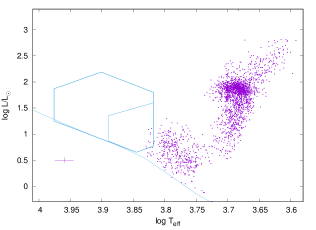
Figure 1: The location of stars with solar-like oscillations from Huber et al. (2017) in the H-R diagram. The zero-age main sequence for models of solar abundance from Bertelli et al. (2008) is shown (solid line). The large polygonal region shows the location of $\delta$ Sct stars from Balona (2018). The smaller polygon shows the location of the $\gamma$ Dor stars. The cross at bottom left indicates 1-$\sigma$ error bars in effective temperature and luminosity.

3 Detection method

Solar-like oscillations are usually detected by searching for the typical bell-shaped amplitude envelope in the power spectrum of the light curve. Most methods use a smoothed power spectrum to obtain the global parameters of the Gaussian envelope. A model consisting of the background, which includes a contribution from granulation, and a Gaussian is then fitted to the data and tested for significance. The peak of the Gaussian gives $\nu_{\rm max}$ while $\Delta\nu$ is estimated by autocorrelation. This procedure and variants are described in, for example, Gilliland et al. (1993); Mosser & Appourchaux (2009); Huber et al. (2009); Mathur et al. (2010); Benomar et al. (2012); Lund et al. (2012).

All methods make use of the well-known asymptotic formula for p modes (Tassoul, 1980):

$$\nu_{nl}\approx\Delta\nu\left(n+\tfrac{1}{2}l+\epsilon\right)-l(l+1)D_{0},$$

where $l$ is the spherical harmonic number of the mode and $n$ is its radial order. The constant $\epsilon$ is sensitive to the surface layers and $D_{0}$ is sensitive to the sound speed gradient near the core. This equation is valid for non-rotating stars and leads to an approximately repetitive frequency pattern with characteristic frequency of $\tfrac{1}{2}\Delta\nu$. The factor of half comes from the fact that the $l=1$ frequency peaks are approximately midway between consecutive radial ($l=0$) peaks. In a star with solar-like oscillations one would expect to find a regular frequency spacing of $\tfrac{1}{2}\Delta\nu$ within a restricted frequency range corresponding to the location of bell-shaped amplitude distribution centered at $\nu_{\rm max}$. Several reviews on solar-like oscillations are available (Chaplin & Miglio, 2013; García & Ballot, 2019; Aerts, 2019).

Rotation will introduce splitting of each mode into $2l+1$ multiplets. However, axisymmetric modes will only be slightly affected for small to moderate rotation, so the repetitive frequency pattern will still be preserved, though degraded somewhat. Because hotter stars tend to be more rapid rotators, the difficulty of detecting solar-like oscillations is expected to increase with increasing effective temperature. In addition, the shorter mode lifetimes lead to broader frequency peaks and lower amplitudes.

The detection of a regular frequency spacing is commonly achieved using the power spectrum of the power spectrum of the light curve or by autocorrelation. The autocorrelation, $R(k)$, is the correlation of a signal with a delayed copy of itself with lag $k$: $R_{k}=\sum y(n)y(n-k)$. The autocorrelation can be obtained from this summation, but for computational purposes it is faster to calculate $R_{k}$ from the inverse FFT of the power spectrum of the power spectrum of the light curve.

Figure 2: Panel (a) shows the amplitude periodogram for KIC 3219634, the arrow indicating $\nu_{\rm max}$. Panel (b) shows the autocorrelation at a frequency of 1000 $\mu$Hz showing a period of about $\tfrac{1}{2}\Delta\nu\approx 27$ $\mu$Hz. Panel (c) shows power spectra of the autocorrelation (after removing the central peak) plotted against frequency (the $\nu$ – $\Delta\nu$ diagram). Panel (d) shows the maximum autocorrelation power as a function of frequency within a 10 percent range of the approximate $\Delta\nu$. The curve is a fitted Gaussian with a maximum at $\nu_{\rm max}=1008.1\pm 2.8$ $\mu$Hz. The average $\Delta\nu$ within $\pm\tfrac{1}{2}$FWHM of the maximum is $54.06\pm 0.18$ $\mu$Hz.

The method used here most closely resembles that of Mathur et al. (2010) in that the presence of equally-spaced frequencies in some region of the power spectrum of the light curve is detected. A suitably small region of the power spectrum of the light curve is selected and the autocorrelation function is calculated. If a pattern of equally-spaced frequencies exists in this region, the autocorrelation function will display a periodic variation with period equal to the frequency separation. The amplitude of the periodic variation depends on the strength of the correlation and follows the bell shape seen in the amplitude envelope of the solar-like oscillations in the power spectrum of the light curve.

The frequency range, $\delta\nu$, of the portion of the power spectrum of the light curve used to calculate the autocorrelation needs careful consideration. We know that $\Delta\nu$ is roughly proportional to $\nu_{\rm max}$ (more accurately, $\Delta\nu\propto\nu_{\rm max}^{s}$ where $s\approx 0.8$, Stello et al. 2009). At high frequencies $\delta\nu$ needs to be large enough to include a few periods in the autocorrelation function. Thus $\delta\nu$ should be at least 2 or 3 times $\Delta\nu$. At low frequencies $\Delta\nu$ will be smaller and hence $\delta\nu$ can be made correspondingly smaller. In other words, the frequency range to be sampled for autocorrelation should be roughly proportional to the frequency, $\nu$, that is being sampled, i.e. $\delta\nu=\alpha\nu$. A value of $\alpha=$ 0.2–0.4 was found to be suitable.

To measure the period of the autocorrelation function, it is convenient to calculate the power spectrum of the autocorrelation. This is actually the same as the power spectrum of the power spectrum of the light curve. However, it was found that removing the large maximum at zero lag, which is always present in the autocorrelation, leads to a cleaner power spectrum. The period of variation in the autocorrelation, if any exists, is given by the inverse of the frequency of the highest peak in the power spectrum of the modified autocorrelation. Its amplitude measures the significance of the period.

In the method used here, the autocorrelation is calculated at equal frequency steps in the power spectrum of the light curve. Let $\nu$ be the central frequency at which the autocorrelation is calculated. The power spectrum of the autocorrelation function is plotted at this frequency. If a solar-like oscillation is present, a significant peak will occur in this power spectrum at a period given by $\tfrac{1}{2}\Delta\nu$. By plotting the power spectra at each sampled frequency, $\nu$, a solar oscillation that may be present will be revealed because the maxima of the power spectra will occur at approximately the same period in the power spectrum. It is convenient to plot $\Delta\nu$ itself instead of the period. This $\nu$ – $\Delta\nu$ plot is central to detection of solar-like oscillations.

The value of $\nu_{\rm max}$ will be the value of $\nu$ at which the peak attains maximum amplitude. This can be obtained by sampling the power spectrum of the light curve with smaller frequency steps on a second pass. At each frequency step, the maximum power of the autocorrelation is plotted as a function of $\nu$. This relationship is very close to a Gaussian in most cases, so $\nu_{\rm max}$ may be obtained by fitting a Gaussian to this curve. The uncertainty in $\nu_{\rm max}$ is taken to be the standard deviation of the location of the Gaussian peak obtained from the least-squares fit. Since $\Delta\nu$ is only approximately constant, a best estimate of $\Delta\nu$ is found by taking the mean value within the full-width at half maximum of the Gaussian centered on $\nu_{\rm max}$. The uncertainty in $\Delta\nu$ is taken as the standard deviation of these values.

After a suitable list of candidate stars is compiled and the Lomb-Scargle power spectra calculated, the power spectrum of the modified correlation is plotted as a function of $\Delta\nu$ (the $\nu$ – $\Delta\nu$ plot) using a relatively large frequency step in $\nu$. This plot is examined for the possible presence of a significant peak. As an example, Fig. 2(a) shows the amplitude periodogram of the light curve of KIC 3219634, which is a previously undiscovered solar-like pulsator. The solar-like oscillations are hardly detectable by visual inspection of the periodogram. Fig. 2(b) shows the autocorrelation function near $\nu_{\rm max}$. The periodicity is clearly seen. Fig 2(c) shows part of the $\nu$ - $\Delta\nu$ diagram calculated with a step size of 50 $\mu$Hz in $\nu$. It is clear that equally-spaced frequencies are present at about $\Delta\nu\approx 55$ $\mu$Hz and $\nu_{\rm max}\approx$ 1000 $\mu$Hz. In a second pass, the step size in $\nu$ has been reduced to 10 $\mu$Hz and at each frequency step the maximum power in the modified autocorrelation is measured within a restricted range of $\Delta\nu$. The range was taken to be $\pm 0.1\Delta\nu$. A Gaussian fitted to the larger peak gives the best estimate of $\nu_{\rm max}$.

The detection of the “humps” which represent a region of high autocorrelation is never a problem as they always have high signal-to-noise. The example of Fig. 2(c) is fairly typical. The main problem is that for some stars many similar humps and/or ridges are visible. For example, eclipsing binaries have significant power at large harmonics which appear as ridges in the $\nu$ — $\Delta\nu$ diagram. Although these cannot be mistaken for the hump characteristic of solar-like oscillations, it interferes with detection of such a hump. Pulsating stars, such as $\delta$ Sct/$\gamma$ Dor variables also have ridges in the diagram which tend to confuse the detection of solar-like oscillations. This is the case for HD 187547, the $\delta$ Sct star previously thought to contain solar-like oscillations (Antoci et al., 2011). This means that any solar-like oscillations in $\delta$ Sct stars, if they exist, may be obscured by the ridges created by $\delta$ Sct pulsation in the $\nu$ – $\Delta\nu$ diagram. If a hump lies close to the expected location in ($\nu_{\rm max},\Delta\nu$), it may represent a true oscillation, but one cannot be certain. The method is aimed at finding oscillations with very low amplitudes. This, of course, is what is needed to extend the region where these oscillations are to be found to higher effective temperatures. The price to be paid is that there is a significant risk of a false detection.

4 Results

Of the 2347 stars with $6000<T_{\rm eff}<10000$ K observed in short-cadence mode, solar-like oscillations were detected in 167 stars. This includes the 97 stars in Table 1 (in the Appendix) which were already known to have solar-like oscillations. The fact that all stars with $T_{\rm eff}>6000$ K and with known solar-like oscillations were quite easily detected, lends confidence to the method described above. In addition, Table 2 in the Appendix lists 70 stars with newly-found solar-like oscillations. For all 167 stars, there is no difficulty in locating the hump as it is the only one with significant visibility. The tables give the oscillation parameters as well as the adopted effective temperatures and luminosities derived from Gaia DR2 parallaxes as mentioned above. The median rms error is 1.95 $\mu$Hz in $\nu_{\rm max}$ and 0.31 $\mu$Hz in $\Delta\nu$.

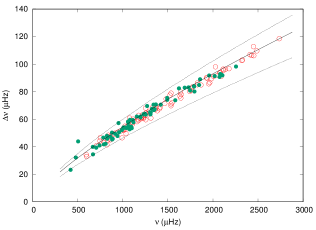
Figure 3: The large separation, $\Delta\nu$, as a function of $\nu_{\rm max}$ for 167 stars. Stars known from the literature are shown by open circles (red), newly detected stars by filled circles (green). The solid line is the relation from Stello et al. (2009) and dotted lines show +10 and -15 per cent deviations.

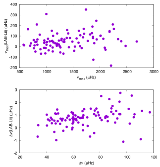
Figure 4: Comparison of $\nu_{\rm max}$ (top panel) and $\Delta\nu$ (bottom panel) obtained in this paper (LAB) with those in the literature.

Fig. 3 shows the large separation, $\Delta\nu$, as a function of $\nu_{\rm max}$ for the 167 stars. The 70 newly discovered stars follow the same relationship as the 97 stars in which solar-like oscillations are known to be present. This is a strong indication that the detected oscillations are real.

Fig. 4 compares the values of $\nu_{\rm max}$ and $\Delta\nu$ obtained here with those in the literature. In both cases, the difference increases with $\nu_{\rm max}$. Neither $\nu_{\rm max}$ or $\Delta\nu$ are well-defined quantities. $\nu_{\rm max}$ is usually estimated by fitting a Gaussian to the envelope of the peaks. $\Delta\nu$ varies slightly with $\nu$ and is normally measured at $\nu_{\rm max}$. In both cases the trend shown in Fig. 4 may be related to the fact that the frequency range, $\delta\nu$, which is sampled to derive the autocorrelation increases with $\nu_{\rm max}$, as described above. In short, the method described here is suited to the detection of low-amplitude signals but is not optimized for a strict evaluation of $\nu_{\rm max}$ and $\Delta\nu$. This clearly requires individual peaks to be resolved.

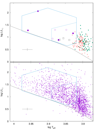
Figure 5: Top panel: the location in the H–R diagram of stars in Tables 1–3. Newly detected stars are shown by the small filled green circles and known stars by small open red circles. The large symbols are stars with possible solar-like oscillations: violet filled circles - non-variable stars; violet open circles: $\delta$ Sct; black squares - $\gamma$ Dor stars. Bottom panel: the small filled circles are from the sample of 2347 stars used to search for solar-like oscillations. The zero-age main sequence for models of solar abundance from Bertelli et al. (2008) is shown (black solid line). The large polygonal region shows the location of $\delta$ Sct stars from Balona (2018). The smaller polygon shows the location of the $\gamma$ Dor stars. The cross at bottom left shows 1-$\sigma$ error bars.

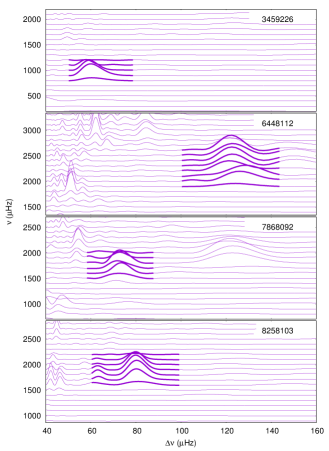
Figure 6: The $\nu$ – $\Delta\nu$ diagrams for the four hottest non-pulsating stars. The thicker solid lines indicate the region which might be a result of solar-like oscillations.

The top panel in Fig. 5 shows the location of the 167 stars with solar-like oscillations in the H-R diagram as well as the $\delta$ Sct and $\gamma$ Dor region of instability from Balona (2018). The bottom panel shows the location of the 2347 stars in our sample. This is to show that there is a uniform decrease of density of stars with increasing $T_{\rm eff}$. There is no abrupt change in stellar density which might be responsible for a sharp decrease in number of stars with solar-like oscillations. In the effective temperature range 6000—6500 K about 17 percent of stars in our sample are solar-like oscillators. If this fraction remains the same for hotter stars, at least 80 solar-like oscillators may be expected just within the $\delta$ Sct instability strip in the temperature range 6500–7000 K.

Two apparently non-pulsating stars KIC 6448112 ($T_{\rm eff}=8498$ K) and KIC 8258103 ($T_{\rm eff}=9082$ K) seem to have a hump in the $\nu$ – $\Delta\nu$ diagram which might be a result of solar-like oscillations. KIC 7868092 ($T_{\rm eff}=6726$ K) and KIC 3459226 ($T_{\rm eff}=7410$ K) are somewhat cooler non-pulsating stars in which a hump is also visible. In all these stars, no indication of periodogram peaks are seen at $\nu_{\rm max}$.

The $\nu$ – $\Delta\nu$ diagrams for these stars are shown in Fig. 6. In every case the detection of possible solar-like oscillations is very tentative because of the presence of similar hump-like features. For this reason, it is not certain that solar-like oscillations are present, even though the measured $\nu_{\rm max}$ and $\Delta\nu$ are consistent with solar-like oscillations.

Indications of solar like oscillations were also detected in three $\delta$ Sct stars (KIC 7212040, KIC5̇476495, KIC 9347095), and three $\gamma$ Dor stars (KIC 9696853, KIC 8264254, KIC 5608334). Once again, many other hump-like features are present as well as ridges in the $\nu$ – $\Delta\nu$ diagram. As before, this greatly reduces the confidence that solar-like oscillations are present. For the sake of completeness, oscillation parameters of these ten stars are given in Table 3 in the Appendix.

5 Discussion and conclusions

In this study an attempt is made to detect solar-like oscillating stars hotter than 6000 K in order to determine the hot edge of the excitation of solar-like oscillations in main sequence stars. The temperature region examined includes the $\delta$ Sct/$\gamma$ Dor instability strip. Discovery of solar-like oscillations in $\delta$ Sct stars would, of course, be of great interest. There are also large numbers of non-pulsating stars within the $\delta$ Sct/$\gamma$ Dor instability strip. Detecting solar-like oscillations in these stars would be much easier than in $\delta$ Sct or $\gamma$ Dor stars because the low-amplitude of solar-like oscillations is likely to be swamped by the much higher amplitudes of self-driven modes.

In order to improve the detection probability, a simple method of detecting solar-like oscillations of low amplitudes (well below the level of detection by inspection of the periodogram) was devised. However, the method does have a significant risk of a false detection. The method does not require smoothing of the periodogram or fitting of a granulation model. In this method, a search is made for equal frequency spacings using autocorrelation. It is found that the power spectrum of the autocorrelation is a powerful tool which easily allows detection of very low-amplitude solar-like oscillations. This is accomplished by inspecting a plot of the power spectrum as a function of frequency (the $\nu$ – $\Delta\nu$ diagram). In this way, all known solar-like oscillating stars hotter than 6000 K were independently detected without difficulty.

Application of this method to stars with $6000<T_{\rm eff}<10000$ K led to the detection of 70 previously unknown solar-like oscillating stars. None of these stars are located within the $\delta$ Sct/$\gamma$ Dor instability strip. If the fraction of stars with solar-like oscillations is the same on either side of the cool edge of the $\delta$ Sct instability strip, then several dozen such stars should have been detected. There are 77 stars within the $\delta$ Sct instability strip with no apparent variability. These would be the best candidates as there is no interference from self-driven pulsations. Yet solar-like oscillations are not found with certainty in any of these stars.

Some uncertain indication of solar like oscillations were detected in four non-variable stars and six pulsating stars inside the $\delta$ Sct instability strip. However, the detections are not sufficiently convincing. None of these ten stars constitute sufficient proof that the hot edge of solar-like oscillations extends to within the $\delta$ Sct/$\gamma$ Dor instability strip.

It should be noted that the line-widths in the periodogram of main sequence stars with solar-like oscillations increases with effective temperature (White et al., 2012; Lund et al., 2017; Compton et al., 2019). This is a consequence of the shorter stochastic mode lifetimes. Increase of line broadening results in a decrease of line amplitude for oscillations of the same energy. In addition, the rotation rate increases with $T_{\rm eff}$, further complicating the frequency spectrum. As a result, detection of individual modes in these stars becomes increasingly more difficult with increasing $T_{\rm eff}$. However, the characteristic bell-shaped envelope of solar-like oscillations should still be visible. The author has inspected the periodograms of many thousands of $\delta$ Sct stars, but no indication of such a feature has ever been seen.

The conclusion is that the hot edge of solar-like oscillations probably coincides with the cool edge of the $\delta$ Sct/$\gamma$ Dor instability strip. This is quite an interesting coincidence and raises the question of whether the physical factors giving rise to self-driven pulsations also act to damp solar-like oscillations. Further study of this problem would require the precision and time span matching that of the Kepler photometry. Hopefully, this may be attained in the not too distant future.

Appendix

Table 1: Table of known stars with solar-like oscillations. The first column is the KIC number. The values of $\nu_{\rm max}$ ($\mu$Hz) and $\Delta\nu$ ($\mu$Hz) (together with their 1- $\sigma$ errors) follows. The effective temperature, $T_{\rm eff}$ (K), from the literature and the luminosity, $\log{L/L_{\odot}}$, from the Gaia DR2 parallax, are shown. Note that for stars with $T_{\rm eff}>6500$ K, values are from the calibration of Balona et al. (2015).

KIC	$\nu_{\rm max}$	$\Delta\nu$	$T_{\rm eff}$	$\log\tfrac{L}{L_{\odot}}$	KIC	$\nu_{\rm max}$	$\Delta\nu$	$T_{\rm eff}$	$\log\tfrac{L}{L_{\odot}}$
1430163	$1829.0\pm 3.6$	$86.39\pm 0.21$	6588	0.64	8367710	$1107.1\pm 1.2$	$56.40\pm 0.25$	6364	0.88
1435467	$1464.6\pm 1.5$	$71.38\pm 0.40$	6306	0.66	8377423	$1023.0\pm 2.3$	$52.46\pm 0.23$	6141	0.84
1725815	$1009.0\pm 1.7$	$51.96\pm 0.15$	6196	0.85	8408931	$594.3\pm 1.8$	$34.20\pm 0.69$	6143	1.12
2837475	$1633.5\pm 1.1$	$76.80\pm 0.12$	6641	0.74	8420801	$1361.1\pm 3.1$	$67.20\pm 0.38$	6245	0.69
3123191	$2092.3\pm 6.7$	$91.16\pm 0.60$	6450	0.60	8494142	$1174.9\pm 0.7$	$62.77\pm 0.23$	6070	0.69
3236382	$1643.5\pm 3.9$	$75.33\pm 0.65$	6715	0.74	8579578	$946.8\pm 1.2$	$50.64\pm 0.08$	6339	0.91
3344897	$835.0\pm 1.8$	$47.35\pm 0.12$	6434	0.95	8866102	$2118.0\pm 1.4$	$95.57\pm 0.30$	6264	0.51
3424541	$754.0\pm 1.0$	$41.94\pm 0.07$	6123	1.06	8940939	$1535.1\pm 3.3$	$78.91\pm 0.25$	6342	0.77
3456181	$1005.9\pm 1.1$	$52.93\pm 0.29$	6381	0.88	8956017	$1254.5\pm 4.1$	$62.87\pm 0.58$	6397	0.80
3547794	$1327.7\pm 4.5$	$68.37\pm 0.54$	6462	0.77	9116461	$2452.2\pm 3.7$	$106.13\pm 0.39$	6429	0.47
3633889	$2113.0\pm 4.3$	$96.35\pm 0.60$	6328	0.48	9139151	$2735.7\pm 2.6$	$118.47\pm 0.17$	6114	0.30
3733735	$2075.7\pm 1.9$	$93.47\pm 0.13$	6726	0.66	9139163	$1757.8\pm 1.3$	$81.90\pm 0.40$	6403	0.68
3967430	$1981.1\pm 2.9$	$89.30\pm 0.39$	6682	0.63	9163769	$1753.3\pm 4.1$	$80.97\pm 1.47$	6410	0.65
4465529	$1546.7\pm 3.0$	$71.96\pm 0.87$	6344	0.70	9206432	$1953.0\pm 1.6$	$85.69\pm 0.21$	6531	0.67
4586099	$1229.6\pm 1.3$	$62.47\pm 0.46$	6378	0.76	9226926	$1480.3\pm 1.6$	$74.71\pm 0.57$	6736	0.77
4638884	$1231.3\pm 1.1$	$61.44\pm 0.14$	6448	0.82	9287845	$1034.7\pm 3.5$	$49.60\pm 0.43$	6309	0.97
4646780	$1074.5\pm 3.2$	$60.85\pm 0.57$	6628	0.84	9328372	$1406.0\pm 5.4$	$67.59\pm 0.56$	6390	0.84
4931390	$2080.4\pm 1.2$	$93.73\pm 0.12$	6703	0.60	9455860	$1534.3\pm 3.4$	$71.05\pm 0.93$	6579	0.74
5095850	$750.6\pm 7.5$	$46.59\pm 0.59$	6759	1.09	9457728	$1114.4\pm 1.9$	$59.97\pm 0.49$	6284	0.78
5214711	$1310.9\pm 1.7$	$60.78\pm 0.43$	6302	0.73	9542776	$823.8\pm 3.6$	$41.42\pm 0.51$	6435	1.10
5431016	$917.8\pm 0.9$	$49.97\pm 0.26$	6594	0.96	9697131	$1204.2\pm 2.0$	$61.25\pm 0.29$	6337	0.84
5516982	$1827.7\pm 1.4$	$85.02\pm 0.47$	6386	0.57	9812850	$1292.9\pm 1.3$	$65.70\pm 0.39$	6458	0.71
5636956	$1056.8\pm 2.0$	$55.30\pm 0.14$	6436	0.88	9821513	$1230.8\pm 1.7$	$60.66\pm 0.12$	6335	0.77
5773345	$1156.7\pm 1.0$	$58.19\pm 0.28$	6179	0.80	10003270	$792.3\pm 2.5$	$43.07\pm 0.15$	6395	1.02
5961597	$1206.5\pm 1.9$	$60.94\pm 0.11$	6573	0.86	10016239	$2326.8\pm 1.8$	$102.98\pm 0.40$	6277	0.51
6064910	$828.9\pm 1.5$	$44.53\pm 0.23$	6370	0.96	10024648	$1084.7\pm 1.6$	$57.46\pm 0.39$	6258	0.78
6225718	$2410.3\pm 1.4$	$106.89\pm 0.12$	6223	0.36	10070754	$2320.4\pm 3.1$	$102.62\pm 0.38$	6437	0.48
6232600	$2178.2\pm 2.0$	$96.68\pm 0.32$	6447	0.51	10081026	$745.0\pm 2.8$	$44.21\pm 0.08$	6368	1.03
6508366	$998.0\pm 0.9$	$52.31\pm 0.24$	6343	0.87	10273246	$903.6\pm 1.2$	$49.07\pm 0.38$	6155	0.81
6530901	$1639.1\pm 3.2$	$79.79\pm 0.71$	6233	0.63	10351059	$1382.1\pm 3.4$	$66.13\pm 0.27$	6435	0.83
6612225	$1167.1\pm 1.4$	$60.12\pm 0.12$	6309	0.78	10355856	$1366.9\pm 1.7$	$68.06\pm 0.22$	6438	0.76
6679371	$976.1\pm 0.8$	$51.42\pm 0.07$	6302	0.96	10454113	$2428.7\pm 1.3$	$106.34\pm 0.24$	6155	0.51
7103006	$1199.5\pm 1.0$	$60.34\pm 0.26$	6420	0.81	10491771	$1773.9\pm 6.6$	$83.50\pm 0.96$	6491	0.62
7106245	$2448.9\pm 2.3$	$112.73\pm 0.21$	6082	0.21	10709834	$1416.2\pm 1.5$	$68.70\pm 0.11$	6453	0.83
7133688	$1172.7\pm 3.5$	$59.09\pm 0.23$	6383	0.85	10730618	$1343.2\pm 1.1$	$67.11\pm 0.34$	6401	0.81
7206837	$1742.7\pm 1.3$	$80.14\pm 0.42$	6340	0.60	10972252	$863.4\pm 1.9$	$45.05\pm 0.27$	6202	0.93
7218053	$707.0\pm 1.9$	$40.70\pm 0.46$	6366	1.03	11070918	$1253.2\pm 1.5$	$68.04\pm 0.49$	6642	1.22
7282890	$852.0\pm 1.4$	$45.67\pm 0.12$	6345	0.99	11081729	$2009.0\pm 1.8$	$91.10\pm 0.50$	6530	0.61
7465072	$1534.2\pm 3.9$	$69.77\pm 1.35$	6309	0.67	11189107	$992.2\pm 4.8$	$46.47\pm 0.46$	6513	1.03
7529180	$1963.7\pm 2.0$	$86.56\pm 0.20$	6657	0.68	11229052	$1867.5\pm 2.9$	$84.82\pm 0.17$	6376	0.65
7530690	$2027.9\pm 4.4$	$98.02\pm 0.57$	6568	0.61	11253226	$1647.5\pm 1.2$	$78.01\pm 0.15$	6642	0.75
7622208	$1254.0\pm 6.9$	$59.60\pm 0.69$	6396	0.82	11453915	$2486.2\pm 4.5$	$109.58\pm 1.01$	6331	0.33
7670943	$1927.8\pm 1.4$	$90.13\pm 0.20$	6315	0.53	11460626	$839.8\pm 1.9$	$48.39\pm 0.28$	6065	0.81
7800289	$599.0\pm 3.8$	$32.89\pm 0.42$	6455	1.17	11467550	$1023.0\pm 2.9$	$54.89\pm 0.35$	6202	0.76
7938112	$1218.4\pm 4.5$	$63.12\pm 1.03$	6337	0.76	11757831	$1256.3\pm 2.7$	$64.35\pm 0.43$	6468	0.86
8150065	$1933.7\pm 1.6$	$89.76\pm 0.17$	6263	0.49	11919192	$866.2\pm 1.8$	$47.82\pm 0.33$	6448	1.00
8179536	$2138.5\pm 1.6$	$96.27\pm 0.28$	6347	0.47	12156916	$1523.4\pm 1.9$	$77.53\pm 0.24$	6438	0.58
8216936	$1110.1\pm 2.6$	$57.61\pm 0.38$	6419	1.01	12317678	$1254.3\pm 1.3$	$64.42\pm 0.11$	6589	0.83
8298626	$2050.9\pm 3.3$	$91.81\pm 0.20$	6200	0.46

Table 2: Newly-discovered stars with solar-like oscillations. The cloumns are the same as Table 1.

KIC	$\nu_{\rm max}$	$\Delta\nu$	$T_{\rm eff}$	$\log\tfrac{L}{L_{\odot}}$	KIC	$\nu_{\rm max}$	$\Delta\nu$	$T_{\rm eff}$	$\log\tfrac{L}{L_{\odot}}$
3102595	$1074.9\pm 3.3$	$52.65\pm 0.18$	6183	0.79	8279146	$1366.7\pm 3.2$	$70.69\pm 0.34$	6650	0.77
3219634	$1008.1\pm 2.7$	$54.06\pm 0.18$	6286	0.81	8346342	$915.8\pm 0.8$	$49.37\pm 0.30$	6316	0.89
3241299	$1117.6\pm 3.0$	$57.80\pm 0.18$	6316	1.10	8737094	$887.5\pm 2.0$	$45.72\pm 0.18$	6541	1.08
3850086	$989.9\pm 2.5$	$52.09\pm 0.58$	6461	0.92	8801316	$1111.4\pm 2.4$	$59.37\pm 0.11$	6489	0.93
3852594	$1006.4\pm 2.2$	$53.64\pm 0.21$	6417	0.85	8806223	$1729.0\pm 2.9$	$83.09\pm 0.28$	6480	0.62
3936993	$1195.3\pm 4.4$	$61.89\pm 1.33$	6225	0.73	8914779	$1492.6\pm 4.1$	$74.05\pm 0.59$	6258	0.64
4484238	$2080.2\pm 2.1$	$92.80\pm 0.07$	6043	0.56	9109988	$2255.5\pm 5.6$	$98.22\pm 0.23$	6127	0.44
5105070	$1154.8\pm 2.2$	$61.93\pm 0.47$	6090	0.62	9209245	$1092.0\pm 3.4$	$54.61\pm 0.31$	6235	0.77
5183581	$1017.8\pm 1.7$	$53.81\pm 0.19$	6387	0.87	9221678	$1746.4\pm 5.1$	$80.81\pm 0.75$	6281	0.62
5597743	$1060.7\pm 3.3$	$55.07\pm 0.59$	6014	0.84	9412514	$823.3\pm 2.4$	$47.93\pm 0.19$	6075	0.92
5696625	$704.9\pm 2.7$	$39.29\pm 0.18$	6402	1.48	9426660	$1491.9\pm 2.5$	$75.43\pm 0.39$	6157	0.54
5771915	$1420.6\pm 5.3$	$70.55\pm 0.74$	6230	0.68	9529969	$1581.8\pm 3.2$	$73.75\pm 1.50$	6021	0.48
5791521	$669.0\pm 2.7$	$34.45\pm 0.26$	6398	1.35	9715099	$741.9\pm 1.1$	$40.93\pm 0.17$	6217	1.04
5856836	$2104.9\pm 5.0$	$91.87\pm 0.59$	6233	0.48	9837454	$782.9\pm 2.0$	$46.62\pm 0.29$	5912	0.78
5871558	$862.6\pm 2.4$	$47.23\pm 0.28$	6239	0.88	9898385	$1269.3\pm 5.4$	$69.58\pm 0.35$	6257	0.75
5905822	$1686.0\pm 1.7$	$82.86\pm 0.10$	6057	0.50	9959494	$1856.8\pm 3.2$	$88.99\pm 0.17$	6638	0.51
5982353	$940.9\pm 3.3$	$47.77\pm 0.16$	6208	1.04	10010623	$952.3\pm 3.6$	$57.17\pm 0.95$	6532	1.01
6048403	$1039.9\pm 2.0$	$53.58\pm 0.15$	6444	0.89	10208303	$1254.4\pm 2.0$	$63.35\pm 0.43$	6303	0.84
6062024	$1060.7\pm 2.2$	$57.59\pm 0.17$	6166	0.81	10340511	$1957.4\pm 2.9$	$91.73\pm 0.21$	5822	0.36
6268607	$789.7\pm 3.3$	$41.71\pm 0.63$	6208	0.95	10448382	$825.8\pm 1.8$	$45.79\pm 0.23$	5969	0.94
6359801	$1309.2\pm 6.8$	$64.85\pm 1.11$	6463	0.78	10514274	$1098.6\pm 3.5$	$53.47\pm 0.41$	6190	0.84
6761569	$1057.4\pm 1.3$	$58.27\pm 0.34$	6271	0.83	10557075	$1794.6\pm 2.7$	$80.11\pm 0.16$	5825	0.52
6777146	$2090.3\pm 4.9$	$92.55\pm 0.66$	6103	0.47	10775748	$1195.6\pm 1.6$	$61.25\pm 0.29$	6393	0.82
6784857	$1241.9\pm 1.8$	$63.70\pm 0.39$	6172	0.71	10813660	$1846.0\pm 3.0$	$84.82\pm 0.70$	6170	0.50
6881330	$1790.1\pm 3.8$	$84.03\pm 0.26$	6092	0.49	10864215	$478.4\pm 1.6$	$32.16\pm 0.42$	6348	1.21
7205315	$1345.9\pm 5.3$	$66.59\pm 0.50$	6051	0.75	10920182	$1354.1\pm 1.9$	$67.24\pm 0.12$	5957	0.62
7215603	$1790.2\pm 1.9$	$83.65\pm 0.26$	6230	0.54	11137841	$667.2\pm 2.2$	$39.90\pm 0.32$	6406	1.12
7272437	$1229.9\pm 2.2$	$63.62\pm 0.39$	6078	0.70	11230757	$1079.2\pm 2.5$	$59.51\pm 0.41$	6158	0.86
7418476	$1241.8\pm 4.0$	$63.95\pm 0.28$	6725	0.74	11245074	$420.4\pm 1.0$	$23.23\pm 0.34$	6073	1.29
7439300	$809.6\pm 1.6$	$42.15\pm 0.17$	6121	1.03	11255615	$1340.9\pm 1.2$	$70.55\pm 0.19$	6194	0.59
7500061	$1307.3\pm 2.9$	$63.50\pm 0.15$	6265	0.73	11337566	$958.3\pm 1.4$	$50.52\pm 0.40$	6238	0.91
7669332	$503.9\pm 1.8$	$43.87\pm 1.08$	6183	1.13	11769801	$880.9\pm 3.2$	$45.23\pm 0.56$	6389	1.06
7833587	$1302.9\pm 3.0$	$64.91\pm 0.22$	6236	0.72	11862497	$2072.7\pm 3.4$	$90.68\pm 0.39$	6426	0.58
8165738	$1622.5\pm 4.3$	$82.40\pm 1.25$	6331	0.53	11970698	$1324.0\pm 2.3$	$67.54\pm 0.22$	5841	0.62
8243381	$879.8\pm 3.6$	$50.26\pm 1.51$	6101	0.81	12600459	$2019.1\pm 3.5$	$91.33\pm 0.26$	6284	0.48

Table 3: Stars discussed in the text with possible solar-like oscillations. The columns are the same as in Table 1.

KIC	$\nu_{\rm max}$	$\Delta\nu$	$T_{\rm eff}$	$\log\tfrac{L}{L_{\odot}}$	KIC	$\nu_{\rm max}$	$\Delta\nu$	$T_{\rm eff}$	$\log\tfrac{L}{L_{\odot}}$
3459226	$964.8\pm 4.2$	$60.17\pm 1.44$	7410	0.89	7868092	$1709.9\pm 7.6$	$73.31\pm 1.39$	6726	1.16
5476495	$954.7\pm 3.1$	$52.09\pm 0.92$	7582	1.30	8258103	$1866.5\pm 3.3$	$80.83\pm 0.40$	9082	1.28
5608334	$2099.4\pm 12.2$	$97.97\pm 3.61$	6900	0.89	8264254	$1534.6\pm 11.0$	$72.33\pm 3.65$	7174	0.96
6448112	$2343.3\pm 8.4$	$122.80\pm 2.25$	8498	2.06	9347095	$762.2\pm 1.6$	$35.23\pm 0.44$	7035	1.30
7212040	$1313.9\pm 4.4$	$57.29\pm 0.60$	7710	0.94	9696853	$1297.9\pm 8.0$	$66.71\pm 1.78$	7352	0.90

References

- Aerts (2019) Aerts C., 2019, arXiv e-prints, p. arXiv:1912.12300
- Antoci et al. (2011) Antoci V., et al., 2011, Nature, 477, 570
- Antoci et al. (2013) Antoci V., et al., 2013, MNRAS, 435, 1563
- Antoci et al. (2014) Antoci V., et al., 2014, ApJ, 796, 118
- Balona (2018) Balona L. A., 2018, MNRAS, 479, 183
- Balona et al. (2015) Balona L. A., Daszyńska-Daszkiewicz J., Pamyatnykh A. A., 2015, MNRAS, 452, 3073
- Bedding et al. (2020) Bedding T. R., et al., 2020, Nature, 581, 147
- Benomar et al. (2012) Benomar O., Baudin F., Chaplin W. J., Elsworth Y., Appourchaux T., 2012, MNRAS, 420, 2178
- Bertelli et al. (2008) Bertelli G., Girardi L., Marigo P., Nasi E., 2008, A&A, 484, 815
- Borucki et al. (2010) Borucki W. J., et al., 2010, Science, 327, 977
- Brown et al. (1991) Brown T. M., Gilliland R. L., Noyes R. W., Ramsey L. W., 1991, ApJ, 368, 599
- Brown et al. (2011) Brown T. M., Latham D. W., Everett M. E., Esquerdo G. A., 2011, AJ, 142, 112
- Castelli & Kurucz (2003) Castelli F., Kurucz R. L., 2003, in Piskunov N., Weiss W. W., Gray D. F., eds, IAU Symposium Vol. 210, Modelling of Stellar Atmospheres. p. A20
- Chaplin & Miglio (2013) Chaplin W. J., Miglio A., 2013, ARA&A, 51, 353
- Chaplin et al. (2014) Chaplin W. J., et al., 2014, ApJS, 210, 1
- Compton et al. (2019) Compton D. L., Bedding T. R., Stello D., 2019, MNRAS, 485, 560
- Fridlund et al. (2006) Fridlund M., Roxburgh I., Favata F., Volonté S., 2006, in Fridlund M., Baglin A., Lochard J., Conroy L., eds, ESA Special Publication Vol. 1306, The CoRoT Mission Pre-Launch Status - Stellar Seismology and Planet Finding. p. 135
- Gaia Collaboration et al. (2016) Gaia Collaboration et al., 2016, A&A, 595, A1
- Gaia Collaboration et al. (2018) Gaia Collaboration Brown A. G. A., Vallenari A., Prusti T., de Bruijne J. H. J., Babusiaux C., Bailer-Jones C. A. L., 2018, preprint, (arXiv:1804.09365)
- García & Ballot (2019) García R. A., Ballot J., 2019, Living Reviews in Solar Physics, 16, 4
- Gilliland et al. (1993) Gilliland R. L., et al., 1993, AJ, 106, 2441
- Gontcharov (2017) Gontcharov G. A., 2017, Astronomy Letters, 43, 472
- Huber et al. (2009) Huber D., Stello D., Bedding T. R., Chaplin W. J., Arentoft T., Quirion P.-O., Kjeldsen H., 2009, Communications in Asteroseismology, 160, 74
- Huber et al. (2011) Huber D., et al., 2011, ApJ, 743, 143
- Huber et al. (2017) Huber D., et al., 2017, ApJ, 844, 102
- Kallinger et al. (2010) Kallinger T., et al., 2010, A&A, 522, A1
- Kjeldsen et al. (1995) Kjeldsen H., Bedding T. R., Viskum M., Frandsen S., 1995, AJ, 109, 1313
- Leighton et al. (1962) Leighton R. B., Noyes R. W., Simon G. W., 1962, ApJ, 135, 474
- Lund et al. (2012) Lund M. N., Chaplin W. J., Kjeldsen H., 2012, MNRAS, 427, 1784
- Lund et al. (2017) Lund M. N., et al., 2017, ApJ, 835, 172
- Mathur et al. (2010) Mathur S., et al., 2010, A&A, 511, A46
- Mathur et al. (2017) Mathur S., et al., 2017, ApJS, 229, 30
- Mosser & Appourchaux (2009) Mosser B., Appourchaux T., 2009, A&A, 508, 877
- Samadi et al. (2002) Samadi R., Goupil M., Houdek G., 2002, A&A, 395, 563
- Serenelli et al. (2017) Serenelli A., et al., 2017, ApJS, 233, 23
- Smith et al. (2012) Smith J. C., et al., 2012, PASP, 124, 1000
- Stello et al. (2008) Stello D., Bruntt H., Preston H., Buzasi D., 2008, ApJ, 674, L53
- Stello et al. (2009) Stello D., Chaplin W. J., Basu S., Elsworth Y., Bedding T. R., 2009, MNRAS, 400, L80
- Stumpe et al. (2012) Stumpe M. C., et al., 2012, PASP, 124, 985
- Tassoul (1980) Tassoul M., 1980, ApJS, 43, 469
- White et al. (2012) White T. R., et al., 2012, ApJ, 751, L36
- Xiong et al. (2016) Xiong D. R., Deng L., Zhang C., Wang K., 2016, MNRAS, 457, 3163