Federated Doubly Stochastic Kernel Learning
for Vertically Partitioned Data

Abstract

In a lot of real-world data mining and machine learning applications, data are provided by multiple providers and each maintains private records of different feature sets about common entities. It is challenging to train these vertically partitioned data effectively and efficiently while keeping data privacy for traditional data mining and machine learning algorithms. In this paper, we focus on nonlinear learning with kernels, and propose a federated doubly stochastic kernel learning (FDSKL) algorithm for vertically partitioned data. Specifically, we use random features to approximate the kernel mapping function and use doubly stochastic gradients to update the solutions, which are all computed federatedly without the disclosure of data. Importantly, we prove that FDSKL has a sublinear convergence rate, and can guarantee the data security under the semi-honest assumption. Extensive experimental results on a variety of benchmark datasets show that FDSKL is significantly faster than state-of-the-art federated learning methods when dealing with kernels, while retaining the similar generalization performance.

Keywords: Vertical federated learning, kernel learning, stochastic gradient descent, random feature approximation, privacy

1 Introduction

Vertically partitioned data (Skillicorn and Mcconnell, 2008) widely exist in the modern data mining and machine learning applications, where data are provided by multiple (two or more) providers (companies, stakeholders, government departments, etc.) and each maintains the records of different feature sets with common entities. For example, a digital finance company, an E-commerce company, and a bank collect different information about the same person. The digital finance company has access to the online consumption, loan and repayment information. The E-commerce company has access to the online shopping information. The bank has customer information such as average monthly deposit, account balance. If the person submit a loan application to the digital finance company, the digital finance company might evaluate the credit risk to this financial loan by comprehensively utilizing the information stored in the three parts.

However, direct access to the data in other providers or sharing of the data may be prohibited due to legal and commercial reasons. For legal reason, most countries worldwide have made laws in protection of data security and privacy. For example, the European Union made the General Data Protection Regulation (GDPR) (EU, 2016) to protect users’ personal privacy and data security. The recent data breach by Facebook has caused a wide range of protests (Badshah, 2018). For commercial reason, customer data is usually a valuable business asset for corporations. For example, the real online shopping information of customers can be used to train a recommended model which could provide valuable product recommendations to customers. Thus, all of these causes require federated learning on vertically partitioned data without the disclosure of data.

Table 1: Commonly used smooth loss functions for binary classification (BC) and regression (R).

Name of loss	Type of task	Convex	The loss function
Square loss	BC+R	Yes	$L(f(x_{i}),y_{i})=(f(x_{i})-y_{i})^{2}$
Logistic loss	BC	Yes	$L(f(x_{i}),y_{i})=\log(1+\exp(-y_{i}f(x_{i})))$
Smooth hinge loss	BC	Yes	$L(f(x_{i}),y_{i})=\left\{\begin{array}[]{l@{\ }l}\frac{1}{2}-z_{i}\hfil\ &\textrm{if }\ z_{i}\leq 0\\ \frac{1}{2}(1-z_{i})^{2}\hfil\ &\textrm{if }\ 0<z_{i}<1\\ 0\hfil\ &\textrm{if }\ z_{i}\geq 1\end{array}\right.$, where $z_{i}=y_{i}f(x_{i})$.

In the literature, there are many privacy-preserving federated learning algorithms for vertically partitioned data in various applications, for example, cooperative statistical analysis Du and Atallah (2001), linear regression (Gascón et al., 2016; Karr et al., 2009; Sanil et al., 2004; Gascón et al., 2017), association rule-mining (Vaidya and Clifton, 2002), k-means clustering (Vaidya and Clifton, 2003), logistic regression (Hardy et al., 2017; Nock et al., 2018), random forest Liu et al. (2019), XGBoost Cheng et al. (2019) and support vector machine Yu et al. (2006). From the optimization standpoint, Wan et al. (2007) proposed privacy-preservation gradient descent algorithm for vertically partitioned data. Zhang et al. (2018) proposed a feature-distributed SVRG algorithm for high-dimensional linear classification.

However, existing privacy-preservation federated learning algorithms assume the models are implicitly linearly separable, i.e., in the form of $f(x)=g\circ h(x)$ (Wan et al., 2007), where $g$ is any differentiable function, $\{{\mathcal{G}_{1}},{\mathcal{G}_{2}},\ldots,{\mathcal{G}_{q}}\}$ is a partition of the features and $h(x)$ is a linearly separable function of the form of $\sum_{\ell=1}^{q}h^{\ell}(w_{\mathcal{G}_{\ell}},x_{\mathcal{G}_{\ell}})$. Thus, almost all the existing privacy-preservation federated learning algorithms are limited to linear models. However, we know that the nonlinear models often can achieve better risk prediction performance than linear methods. Kernel methods Gu et al. (2018b, 2008, d) are an important class of nonlinear approaches to handle linearly non-separable data. Kernel models usually take the form of $f(x)=\sum_{i}^{N}\alpha_{i}K(x_{i},x)$ which do not satisfy the assumption of implicitly linear separability, where $K(\cdot,\cdot)$ is a kernel function. To the best of our knowledge, PP-SVMV (Yu et al., 2006) is the only privacy-preserving method for learning vertically partitioned data with non-linear kernels. However, PP-SVMV (Yu et al., 2006) needs to merge the local kernel matrices in different workers to a global kernel matrix, which would cause a high communication cost. It is still an open question to train the vertically partitioned data efficiently and scalably by kernel methods while keeping data privacy.

To address this challenging problem, in this paper, we propose a new federated doubly stochastic kernel learning (FDSKL) algorithm for vertically partitioned data. Specifically, we use random features to approximate the kernel mapping function and use doubly stochastic gradients to update kernel model, which are all computed federatedly without revealing the whole data sample to each worker. We prove that FDSKL can converge to the optimal solution in $\mathcal{O}(1/t)$, where $t$ is the number of iterations. We also provide the analysis of the data security under the semi-honest assumption (i.e., Assumption 2). Extensive experimental results on a variety of benchmark datasets show that FDSKL is significantly faster than state-of-the-art federated learning methods when dealing with kernels, while retaining the similar generalization performance.

Contributions. The main contributions of this paper are summarized as follows.

1. Most of existing federated learning algorithms on vertically partitioned data are limited to linearly separable model. Our FDSKL breaks the limitation of implicitly linear separability.

2. To the best of our knowledge, FDSKL is the first federated kernel method which can train vertically partitioned data efficiently and scalably. We also prove that FDSKL can guarantee data security under the semi-honest assumption.

3. Existing doubly stochastic kernel method is limited to the diminishing learning rate. We extend it to constant learning rate. Importantly, we prove that FDSKL with constant learning rate has a sublinear convergence rate.

2 Vertically Partitioned Federated Kernel Learning Algorithm

In this section, we first introduce the federated kernel learning problem, and then give a brief review of doubly stochastic kernel methods. Finally, we propose our FDSKL.

2.1 Problem Statement

Given a training set $\mathcal{S}=\{(x_{i},y_{i})\}_{i=1}^{N}$, where $x_{i}\in\mathbb{R}^{d}$ and $y_{i}\in\{+1,-1\}$ for binary classification or $y_{i}\in\mathbb{R}$ for regression. Let $L(u,y)$ be a scalar loss function which is convex with respect to $u\in\mathbb{R}$. We give several common loss functions in Table 1. Given a positive definite kernel function $K(x^{\prime},x)$ and the associated reproducing kernel Hilbert spaces (RKHS) $\mathcal{H}$ (Berlinet and Thomas-Agnan, 2011). A kernel method tries to find a function $f\in\mathcal{H}$ for solving:

$$\operatorname*{argmin}_{f\in\mathcal{H}}\mathcal{R}(f)=\mathbb{E}_{(x,y)\in\mathcal{S}}L(f(x),y)+\dfrac{\lambda}{2}\|f\|_{\mathcal{H}}^{2}$$ (1)

where $\lambda>0$ is a regularization parameter.

As mentioned previously, in a lot of real-world data mining and machine learning applications, the input of training sample $(x,y)$ is partitioned vertically into $q$ parts, i.e., $x=[x_{\mathcal{G}_{1}},x_{\mathcal{G}_{2}},\ldots,x_{\mathcal{G}_{q}}]$, and $x_{\mathcal{G}_{\ell}}\in\mathbb{R}^{d_{\ell}}$ is stored on the $\ell$-th worker and $\sum_{\ell=1}^{q}d_{\ell}=d$. According to whether the label is included in a worker, we divide the workers into two types: one is active worker and the other is passive worker, where the active worker is the data provider who holds the label of a sample, and the passive worker only has the input of a sample. The active worker would be a dominating server in federated learning, while passive workers play the role of clients (Cheng et al., 2019). We let $D^{\ell}$ denote the data stored on the $\ell$-th worker, where the labels $y_{i}$ are distributed on active workers. $D^{\ell}$ includes parts of labels $\{y_{i}\}_{i=1}^{l}$. Thus, our goal in this paper can be presented as follows.

Goal: Make active workers to cooperate with passive workers to solve the nonlinear learning problem (1) on the vertically partitioned data $\{D^{\ell}\}_{\ell=1}^{q}$ while keeping the vertically partitioned data private.

Principle of FDSKL. Rather than dividing a kernel into several sub-matrices, which requires expensive kernel merging operation, FDSKL uses the random feature approximation to achieve efficient computation parallelism under the federated learning setting. The efficiency of FDSKL is owing to the fact that the computation of random features can be linearly separable. Doubly stochastic gradient (DSG) Gu et al. (2018a, 2019) is a scalable and efficient kernel method (Dai et al., 2014; Xie et al., 2015; Gu et al., 2018c) which uses the doubly stochastic gradients w.r.t. samples and random features to update the kernel function. We extend DSG to the vertically partitioned data, and propose FDSKL. Specifically, each FDSKL worker computes a partition of the random features using only the partition of data it keeps. When computing the global functional gradient of the kernel, we could efficiently reconstruct the entire random features from the local workers. Note that although FDSKL is also a privacy-preservation gradient descent algorithm for vertically partitioned data, FDSKL breaks the limitation of implicit linear separability used in the existing privacy-preservation federated learning algorithms as discussed previously.

2.2 Brief Review of Doubly Stochastic Kernel Methods

We first introduce the technique of random feature approximation, and then give a brief review of DSG algorithm.

2.2.1 Random Feature Approximation

Random feature (Rahimi and Recht, 2008, 2009; Gu et al., 2018a; Geng et al., 2019; Shi et al., 2019, 2020) is a powerful technique to make kernel methods scalable. It uses the intriguing duality between positive definite kernels which are continuous and shift invariant (i.e., $K(x,x^{\prime})=K(x-x^{\prime})$) and stochastic processes as shown in Theorem 1.

Theorem 1 (Rudin (1962))

A continuous, real-valued, symmetric and shift-invariant function $K(x,x^{\prime})=K(x-x^{\prime})$ on $\mathbb{R}^{d}$ is a positive definite kernel if and only if there is a finite non-negative measure $\mathbb{P}(\omega)$ on $\mathbb{R}^{d}$, such that

$$K(x-x^{\prime})=\int_{\mathbb{R}^{d}}e^{i\omega^{T}(x-x^{\prime})}d\mathbb{P}(\omega)=\int_{\mathbb{R}^{d}\times[0,2\pi]}2\cos(\omega^{T}x+b)\cos(\omega^{T}x^{\prime}+b)d(\mathbb{P}(\omega)\times\mathbb{P}(b))$$ (2)

where $\mathbb{P}(b)$ is a uniform distribution on $[0,2\pi]$, and $\phi_{\omega}(x)=\sqrt{2}\cos(\omega^{T}x+b)$.

According to Theorem 1, the value of the kernel function can be approximated by explicitly computing the random feature maps $\phi_{\omega}(x)$ as follows.

$$K(x,x^{\prime})\approx\frac{1}{m}\sum_{i=1}^{m}\phi_{\omega_{i}}(x)\phi_{\omega_{i}}(x^{\prime})$$ (3)

where $m$ is the number of random features and $\omega_{i}$ are drawn from $\mathbb{P}(\omega)$. Specifically, for Gaussian RBF kernel $K(x,x^{\prime})=\exp(-||x-x^{\prime}||^{2}/2\sigma^{2})$, $\mathbb{P}(\omega)$ is a Gaussian distribution with density proportional to $\exp(-\sigma^{2}\|\omega\|^{2}/2)$. For the Laplace kernel (Yang et al., 2014), this yields a Cauchy distribution. Notice that the computation of a random feature map $\phi$ requires to compute a linear combination of the raw input features, which can also be partitioned vertically. This property makes random feature approximation well-suited for the federated learning setting.

2.2.2 Doubly Stochastic Gradient

Because the functional gradient in RKHS $\mathcal{H}$ can be computed as $\nabla f(x)=K(x,\cdot)$, the stochastic gradient of $\nabla f(x)$ w.r.t. the random feature $\omega$ can be denoted by (4).

$$\xi(\cdot)=\phi_{\omega}(x)\phi_{\omega}(\cdot)$$ (4)

Given a randomly sampled data instance $(x,y)$, and a random feature $\omega$, the doubly stochastic gradient of the loss function $L(f(x_{i}),y_{i})$ on RKHS w.r.t. the sampled instance $(x,y)$ and the random direction $\omega$ can be formulated as follows.

$$\zeta(\cdot)=L^{\prime}(f(x_{i}),y_{i})\phi_{\omega}(x_{i})\phi_{\omega}(\cdot)$$ (5)

Because $\nabla||f||^{2}_{\mathcal{H}}=2f$, the stochastic gradient of $\mathcal{R}(f)$ can be formulated as follows.

$$\widehat{\zeta}(\cdot)=\zeta(\cdot)+\lambda f(\cdot)=L^{\prime}(f(x_{i}),y_{i})\phi_{\omega_{i}}(x_{i})\phi_{\omega_{i}}(\cdot)+\lambda f(\cdot)$$ (6)

Note that we have $\mathbb{E}_{(x,y)}\mathbb{E}_{\omega}\widehat{\zeta}(\cdot)=\nabla\mathcal{R}(f)$. According to the stochastic gradient (6), we can update the solution by stepsize $\gamma_{t}$. Then, let $f_{1}(\cdot)=\textbf{0}$, we have that

$$f_{t+1}(\cdot)= f_{t}(\cdot)-\gamma_{t}\left(\zeta(\cdot)+\lambda f(\cdot)\right)=\sum_{i=1}^{t}-\gamma_{i}\prod_{j=i+1}^{t}(1-\gamma_{j}\lambda)\zeta_{i}(\cdot)$$ (7)

$$= \sum_{i=1}^{t}\underbrace{-\gamma_{i}\prod_{j=i+1}^{t}(1-\gamma_{j}\lambda)L^{\prime}(f(x_{i}),y_{i})\phi_{\omega_{i}}(x_{i})}_{\alpha_{i}^{t}}\phi_{\omega_{i}}(\cdot)$$

From (7), $\alpha_{i}^{t}$ are the important coefficients which defines the model of $f(\cdot)$. Note that the model $f(x)$ in (7) do not satisfy the assumption of implicitly linear separability same to the kernel model $f(x)=\sum_{i}^{N}\alpha_{i}K(x_{i},x)$ as mentioned in the first section.

2.3 Federated Doubly Stochastic Kernel Learning Algorithm

We first present the system structure of FDSKL, and then give a detailed description of FDSKL.

2.3.1 System Structure

As mentioned before, FDSKL is a federated learning algorithm where each worker keeps its local vertically partitioned data. Figure 1 presents the system structure of FDSKL. The main idea behind FDSKL’s parallelism is to vertically divide the computation of the random features. Specifically, we give detailed descriptions of data privacy, model privacy and tree-structured communication, respectively, as follows.

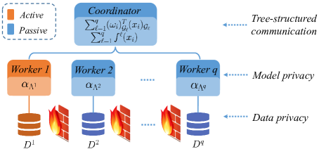
Figure 1: System structure of FDSKL.

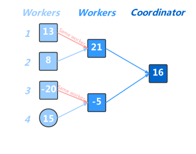
(a) Tree structure $T_{1}$ on workers $\{1,\ldots,4\}$

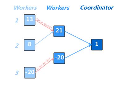
(b) Tree structure $T_{2}$ on workers $\{1,\ldots,3\}$

Figure 2: Illustration of tree-structured communication with two totally different tree structures $T_{1}$ and $T_{2}$.

1. Data Privacy:   To keep the vertically partitioned data privacy, we need to divide the computation of the value of $\phi_{\omega_{i}}(x_{i})=\sqrt{2}\cos(\omega_{i}^{T}x_{i}+b)$ to avoid transferring the local data $(x_{i})_{\mathcal{G}_{\ell}}$ to other workers. Specifically, we send a random seed to the $\ell$-th worker. Once the $\ell$-th worker receive the random seed, it can generate the random direction $\omega_{i}$ uniquely according to the random seed. Thus, we can locally compute $(\omega_{i})_{\mathcal{G}_{\ell}}^{T}(x_{i})_{\mathcal{G}_{\ell}}+b$ which avoids directly transferring the local data $(x_{i})_{\mathcal{G}_{\ell}}$ to other workers for computing $\omega_{i}^{T}x_{i}+b$. In the next section, we will discuss it is hard to infer any $(x_{i})_{\mathcal{G}_{\ell}}$ according to the value of $(\omega_{i})_{\mathcal{G}_{\ell}}^{T}(x_{i})_{\mathcal{G}_{\ell}}+b$ from other workers.

2. Model Privacy:  In addition to keep the vertically partitioned data privacy, we also keep the model privacy. Specifically, the model coefficients $\alpha_{i}$ are stored in different workers separately and privately. According to the location of the model coefficients $\alpha_{i}$, we partition the model coefficients $\{\alpha_{i}\}_{i=1}^{T}$ as $\{\alpha_{\Lambda^{\ell}}\}_{\ell=1}^{q}$, where $\alpha_{\Lambda^{\ell}}$ denotes the model coefficients at the $\ell$-th worker, and $\Lambda^{\ell}$ is the set of corresponding iteration indices. We do not directly transfer the local model coefficients $\alpha_{\Lambda^{\ell}}$ to other workers. To compute $f(x)$, we locally compute $f^{\ell}(x)=\sum_{i\in\Lambda^{\ell}}\alpha_{i}\phi_{\omega_{i}}(x)$ and transfer it to other worker, and $f(x)$ can be reconstructed by summing over all the $f^{\ell}(x)$. It is difficult to infer the the local model coefficients $\alpha_{\Lambda^{\ell}}$ based on the value of $f^{\ell}(x)$ if $|\Lambda^{\ell}|\geq 2$. Thus, we achieve the model privacy.

3. Tree-Structured Communication:  In order to obtain $\omega_{i}^{T}x_{i}$ and $f(x_{i})$, we need to accumulate the local results from different workers. Zhang et al. (2018) proposed an efficient tree-structured communication scheme to get the global sum which is faster than the simple strategies of star-structured communication (Wan et al., 2007) and ring-structured communication (Yu et al., 2006). Take 4 workers as an example, we pair the workers so that while worker 1 adds the result from worker 2, worker 3 can add the result from worker 4 simultaneously. Finally, the results from the two pairs of workers are sent to the coordinator and we obtain the global sum (please see Figure 2(a)). If the above procedure is in a reverse order, we call it a reverse-order tree-structured communication. Note that both of the tree-structured communication scheme and its reverse-order scheme are synchronous procedures.

2.3.2 Algorithm

To extend DSG to federated learning on vertically partitioned data while keeping data privacy, we need to carefully design the procedures of computing $\omega_{i}^{T}x_{i}+b$, $f(x_{i})$ and the solution updates, which are presented in detail as follows.

1. Computing $\omega_{i}^{T}x_{i}+b$:   We generate the random direction $\omega_{i}$ according to a same random seed $i$ and a probability measure $\mathbb{P}$ for each worker. Thus, we can locally compute $(\omega_{i})_{\mathcal{G}_{\ell}}^{T}(x_{i})_{\mathcal{G}_{\ell}}$. To keep $(x_{i})_{\mathcal{G}_{\ell}}$ private, instead of directly transferring $(\omega_{i})_{\mathcal{G}_{\ell}}^{T}(x_{i})_{\mathcal{G}_{\ell}}$ to other workers, we randomly generate $b^{\ell}$ uniformly from $[0,2\pi]$, and transfer $(\omega_{i})_{\mathcal{G}_{\ell}}^{T}(x_{i})_{\mathcal{G}_{\ell}}+b^{\ell}$ to another worker. After all workers have calculated $(\omega_{i})_{\mathcal{G}_{\ell}}^{T}(x_{i})_{\mathcal{G}_{\ell}}+b^{\ell}$ locally, we can get the global sum $\sum_{\hat{\ell}=1}^{q}\left((\omega_{i})_{\mathcal{G}_{\hat{\ell}}}^{T}(x_{i})_{\mathcal{G}_{\hat{\ell}}}+b^{\hat{\ell}}\right)$ efficiently and safely by using a tree-structured communication scheme based on the tree structure $T_{1}$ for workers $\{1,\ldots,q\}$ (Zhang et al., 2018).

   Currently, for the $\ell$-th worker, we get multiple values of $b$ with $q$ times. To recover the value of $\sum_{\hat{\ell}=1}^{q}\left((\omega_{i})_{\mathcal{G}_{\hat{\ell}}}^{T}(x_{i})_{\mathcal{G}_{\hat{\ell}}}\right)+b$, we pick up one $b^{\ell^{\prime}}$ from $\{1,\ldots,q\}-\{\ell\}$ as the value of $b$ by removing other values of $b^{\ell}$ (i.e., removing $\overline{b}^{\ell^{\prime}}=\sum_{{{\hat{\ell}}}\neq\ell^{\prime}}b^{{{\hat{\ell}}}}$). In order to prevent leaking any information of $b^{\ell}$, we use a totally different tree structure $T_{2}$ for workers $\{1,\ldots,q\}-\{\ell^{\prime}\}$ (please see Definition 2 and Figure 2) to compute $\overline{b}^{\ell^{\prime}}=\sum_{{{\hat{\ell}}}\neq\ell^{\prime}}b^{{{\hat{\ell}}}}$. The detailed procedure of computing $\omega_{i}^{T}x_{i}+b$ is summarized in Algorithm 3.

   Definition 2 (Two totally different tree structures)

   For two tree structures $T_{1}$ and $T_{2}$, they are totally different if there does not exist a subtree with more than one leaf which belongs to both of $T_{1}$ and $T_{2}$.

2. Computing $f(x_{i})$:  According to (7), we have that $f(x_{i})=\sum_{i=1}^{t}\alpha_{i}^{t}\phi_{\omega_{i}}(x_{i})$. However, $\alpha_{i}^{t}$ and $\phi_{\omega_{i}}(x_{i})$ are stored in different workers. Thus, we first locally compute $f^{\ell}(x_{i})=\sum_{i\in\Lambda^{\ell}}\alpha_{i}^{t}\phi_{\omega_{i}}(x_{i})$ which is summarized in Algorithm 2. By using a tree-structured communication scheme (Zhang et al., 2018), we can get the global sum $\sum_{\ell=1}^{q}f^{\ell}(x_{i})$ efficiently which is equal to $f(x_{i})$ (please see Line 7 in Algorithm 1).

3. Updating Rules:  Because $\alpha_{i}^{t}$ are stored in different workers, we use a communication scheme (Zhang et al., 2018) with a reverse-order tree structure to update $\alpha_{i}^{t}$ in each workers by the coefficient $(1-\gamma\lambda)$ (please see Line 10 in Algorithm 1).

Based on these key procedures, we summarize our FDSKL algorithm in Algorithm 1. Different to the diminishing learning rate used in DSG, our FDSKL uses a constant learning rate $\gamma$ which can be implemented more easily in the parallel computing environment. However, the convergence analysis for constant learning rate is more difficult than the one for diminishing learning rate. We give the theoretic analysis in the following section.

Algorithm 1 Vertically Partitioned Federated Kernel Learning Algorithm (FDSKL) on the $\ell$-th active worker

0:  $\mathbb{P}(\omega)$, local normalized data $D^{\ell}$, regularization parameter $\lambda$, constant learning rate $\gamma$.

1:  keep doing in parallel

2:      Pick up an instance $(x_{i})_{\mathcal{G}_{\ell}}$ from the local data $D^{\ell}$ with index $i$.

3:      Send $i$ to other workers using a reverse-order tree structure $T_{0}$.

4:      Sample $\omega_{i}\sim\mathbb{P}(\omega)$ with the random seed $i$ for all workers.

5:      Use Algorithm 3 to compute $\omega_{i}^{T}x_{i}+b$ and locally save it.

6:      Compute $f^{\ell^{\prime}}(x_{i})$ for $\ell^{\prime}=1,\ldots,q$ by calling Algorithm 2.

7:      Use tree-structured communication scheme based on $T_{0}$ to compute $f(x_{i})=\sum_{\ell=1}^{q}f^{\ell}(x_{i})$.

8:      Compute $\phi_{\omega_{i}}(x_{i})$ according to $\omega_{i}^{T}x_{i}+b$.

9:      Compute $\alpha_{i}=-\gamma\left(L^{\prime}(f(x_{i}),y_{i})\phi_{\omega_{i}}(x_{i})\right)$ and locally save $\alpha_{i}$.

10:      Update $\alpha_{j}=(1-\gamma\lambda)\alpha_{j}$ for all previous $j$ in the $\ell$-th worker and other workers.

11:  end parallel loop

11:  $\alpha_{\Lambda^{\ell}}$.

Algorithm 2 Compute $f^{\ell}(x)$ on the $\ell$-th active worker

0:  $\mathbb{P}(\omega)$, $\alpha_{\Lambda^{\ell}}$, $\Lambda^{\ell}$, $x$.

1:   Set $f^{\ell}(x)=0$.

2:  for each $i\in\Lambda^{\ell}$ do

3:      Sample $\omega_{i}\sim\mathbb{P}(\omega)$ with the random seed $i$ for all workers.

4:      Obtain $\omega_{i}^{T}x+b$ if it is locally saved, otherwise compute $\omega_{i}^{T}x+b$ by using Algorithm 3.

5:      Compute $\phi_{\omega_{i}}(x)$ according to $\omega_{i}^{T}x+b$.

6:      $f^{\ell}(x)=f^{\ell}(x)+\alpha_{i}\phi_{\omega_{i}}(x)$

7:  end for

7:  $f^{\ell}(x)$

Algorithm 3 Compute $\omega_{i}^{T}x_{i}+b$ on the $\ell$-th active worker

0:  $\omega_{i}$, $x_{i}$ {// This loop asks multiple workers running in parallel.}

1:  for $\hat{\ell}=1,\ldots,q$ do

2:      Compute $(\omega_{i})_{\mathcal{G}_{\hat{\ell}}}^{T}(x_{i})_{\mathcal{G}_{\hat{\ell}}}$ and randomly generate a uniform number $b^{\hat{\ell}}$ from $[0,2\pi]$ with the seed $\sigma^{\hat{\ell}}(i)$.

3:      Calculate $(\omega_{i})_{\mathcal{G}_{\hat{\ell}}}^{T}(x_{i})_{\mathcal{G}_{\hat{\ell}}}+b^{\hat{\ell}}$.

4:  end for

5:   Use tree-structured communication scheme based on the tree structure $T_{1}$ for workers $\{1,\ldots,q\}$ to compute $\xi=\sum_{\hat{\ell}=1}^{q}\left((\omega_{i})_{\mathcal{G}_{\hat{\ell}}}^{T}(x_{i})_{\mathcal{G}_{\hat{\ell}}}+b^{\hat{\ell}}\right)$.

6:   Pick up $\ell^{\prime}\in\{1,\ldots,q\}-\{\ell\}$ uniformly at random.

7:   Use tree-structured communication scheme based on the totally different tree structure $T_{2}$ for workers $\{1,\ldots,q\}-\{\ell^{\prime}\}$ to compute $\overline{b}^{\ell^{\prime}}=\sum_{{\hat{\ell}}\neq\ell^{\prime}}b^{{\hat{\ell}}}$.

7:  $\xi-\overline{b}^{\ell^{\prime}}$.

3 Theoretical Analysis

In this section, we provide the convergence, security and complexity analyses to FDSKL.

3.1 Convergence Analysis

As the basis of our analysis, our first lemma states that the output of Algorithm 3 is actually equal to $\omega_{i}^{T}x+b$. The proofs are provided in Appendix.

Lemma 3

The output of Algorithm 3 (i.e., $\sum_{\hat{\ell}=1}^{q}\left((\omega_{i})_{\mathcal{G}_{\hat{\ell}}}^{T}(x)_{\mathcal{G}_{\hat{\ell}}}+b^{\hat{\ell}}\right)-\overline{b}^{\ell^{\prime}}$ is equal to $\omega_{i}^{T}x+b$, where each $b^{\hat{\ell}}$ and $b$ are drawn from a uniform distribution on $[0,2\pi]$, $\overline{b}^{\ell^{\prime}}=\sum_{{\hat{\ell}}\neq\ell^{\prime}}b^{{\hat{\ell}}}$, and $\ell^{\prime}\in\{1,\ldots,q\}-\{\ell\}$.

Based on Lemma 1, we can conclude that the federated learning algorithm (i.e., FDSKL) can produce the same doubly stochastic gradients as that of a DSG algorithm with constant learning rate. Thus, under Assumption 1, we can prove that FDSKL converges to the optimal solution almost at a rate of $\mathcal{O}(1/t)$ as shown in Theorem 4. The proof is provided in Appendix, Note that the convergence proof of the original DSG algorithm in (Dai et al., 2014) is limited to diminishing learning rate.

Assumption 1

Suppose the following conditions hold.

1. There exists an optimal solution, denoted as $f_{*}$, to the problem (1).

2. We have an upper bound for the derivative of $L(u,y)$ w.r.t. its 1st argument, i.e., $|L^{\prime}(u,y)|<M$.

3. The loss function $L(u,y)$ and its first-order derivative are $\mathcal{L}$-Lipschitz continuous in terms of the first argument.

4. We have an upper bound $\kappa$ for the kernel value, i.e., $K(x,x^{\prime})\leq\kappa$. We have an upper bound $\phi$ for random feature mapping, i.e., $|\phi_{\omega}(x)\phi_{\omega}(x^{\prime})|\leq\phi$.

Theorem 4

Set $\epsilon>0$, $\min\{\frac{1}{\lambda},\frac{\epsilon\lambda}{4M^{2}(\sqrt{\kappa}+\sqrt{\phi})^{2}}\}>\gamma>0$, for Algorithm 1, with $\gamma=\frac{\epsilon\vartheta}{8\kappa B}$ for $\vartheta\in\left(\right.0,1\left.\right]$, under Assumption 1, we will reach $\mathbb{E}\Big{[}|f_{t}(x)-f_{*}(x)|^{2}\Big{]}\leq\epsilon$ after

$$t\geq\frac{8\kappa B\log(8\kappa e_{1}/\epsilon)}{\vartheta\epsilon\lambda}$$ (8)

iterations, where $B=\left[\sqrt{G_{2}^{2}+G_{1}}+G_{2}\right]^{2}$, $G_{1}=\frac{2\kappa M^{2}}{\lambda}$, $G_{2}=\frac{\kappa^{1/2}M(\sqrt{\kappa}+\sqrt{\phi})}{2\lambda^{3/2}}$ and $e_{1}=\mathbb{E}[\|h_{1}-f_{*}\|_{\mathcal{H}}^{2}]$.

Remark 5

Based on Theorem 4, we have that for any given data $x$, the evaluated value of $f_{t+1}$ at $x$ will converge to that of a solution close to $f_{*}$ in terms of the Euclidean distance. The rate of convergence is almost $\mathcal{O}(1/t)$, if eliminating the $\log(1/\epsilon)$ factor. Even though our algorithm has included more randomness by using random features, this rate is nearly the same as standard SGD. As a result, this guarantees the efficiency of the proposed algorithm.

Table 2: The state-of-the-art kernel methods compared in our experiments. (BC=binary classification, R=regression)

Algorithm	Reference	Problem	Vertically Partitioned Data	Doubly Stochastic
LIBSVM	Chang and Lin (2011)	BC+R	No	No
DSG	Dai et al. (2014)	BC+R	No	Yes
PP-SVMV	Yu et al. (2006)	BC+R	Yes	No
FDSKL	Our	BC+R	Yes	Yes

3.2 Security Analysis

We discuss the data security (in other words, prevent local data on one worker leaked to or inferred by other workers) of FDSKL under the semi-honest assumption. Note that the semi-honest assumption is commonly used in in security analysis (Wan et al., 2007; Hardy et al., 2017; Cheng et al., 2019).

Assumption 2 (Semi-honest security)

All workers will follow the protocol or algorithm to perform the correct computations. However, they may retain records of the intermediate computation results which they may use later to infer the data of other workers.

Because each worker knows the parameter $\omega$ given a random seed, we can have a linear system of $o_{j}=(\omega_{j})_{\mathcal{G}_{\ell}}^{T}(x_{i})_{\mathcal{G}_{\ell}}$ with a sequence of trials of $\omega_{j}$ and $o_{j}$. It has the potential to infer $(x_{i})_{\mathcal{G}_{\ell}}$ from the linear system of $o_{j}=(\omega_{j})_{\mathcal{G}_{\ell}}^{T}(x_{i})_{\mathcal{G}_{\ell}}$ if the sequence of $o_{j}$ is also known. We call it inference attack. Please see its formal definition in Definition 6. In this part, we will prove that FDSKL can prevent inference attack (i.e., Theorem 7).

Definition 6 (Inference attack)

An inference attack on the $\ell$-th worker is to infer a certain feature group $\mathcal{G}$ of sample $x_{i}$ which belongs to other workers without directly accessing it.

Theorem 7

Under the semi-honest assumption, the FDSKL algorithm can prevent inference attack.

As discussed above, the key of preventing the inference attack is to mask the value of $o_{j}$. As described in lines 2-3 of Algorithm 3, we add an extra random variable $b^{\hat{\ell}}$ into $(\omega_{j})_{\mathcal{G}_{\ell}}^{T}(x_{i})_{\mathcal{G}_{\ell}}$. Each time, the algorithm only transfers the value of $(\omega_{i})_{\mathcal{G}_{\ell}}^{T}(x_{i})_{\mathcal{G}_{\ell}}+b^{\hat{\ell}}$ to another worker. Thus, it is impossible for the receiver worker to directly infer the value of $o_{j}$. Finally, the $\ell$-th active worker gets the global sum $\sum_{\hat{\ell}=1}^{q}\left((\omega_{i})_{\mathcal{G}_{\hat{\ell}}}^{T}(x_{i})_{\mathcal{G}_{\hat{\ell}}}+b^{\hat{\ell}}\right)$ by using a tree-structured communication scheme based on the tree structure $T_{1}$. Thus, lines 2-4 of Algorithm 3 keeps data privacy.

As proved in Lemma 1, lines 5-7 of Algorithm 3 is to get $\omega_{i}^{T}x+b$ by removing $\overline{b}^{\ell^{\prime}}=\sum_{{{\hat{\ell}}}\neq\ell^{\prime}}b^{{{\hat{\ell}}}}$ from the sum $\sum_{\hat{\ell}=1}^{q}\left((\omega_{i})_{\mathcal{G}_{\hat{\ell}}}^{T}(x_{i})_{\mathcal{G}_{\hat{\ell}}}+b^{\hat{\ell}}\right)$. To prove that FDSKL can prevent the inference attack, we only need to prove that the calculation of $\overline{b}^{\ell^{\prime}}=\sum_{{{\hat{\ell}}}\neq\ell^{\prime}}b^{{{\hat{\ell}}}}$ in line 7 of Algorithm 3 does not disclose the value of $b^{{{\hat{\ell}}}}$ or the sum of $b^{{{\hat{\ell}}}}$ on a node of tree $T_{1}$, which is indicated in Lemma 2 (the proof is provided in Appendix).

Lemma 8

In Algorithm 3, if $T_{1}$ and $T_{2}$ are totally different tree structures, for any worker ${\hat{\ell}}$, there is no risk to disclose the value of $b^{{{\hat{\ell}}}}$ or the sum of $b^{{{\hat{\ell}}}}$ to other workers.

3.3 Complexity Analysis

The computational complexity for one iteration of FDSKL is $\mathcal{O}(dqt)$. The total computational complexity of FDSKL is $\mathcal{O}(dqt^{2})$. Further, the communication cost for one iteration of FDSKL is $\mathcal{O}(qt)$, and the total communication cost of FDSKL is $\mathcal{O}(qt^{2})$. The details of deriving the computational complexity and communication cost of FDSKL are provided in Appendix.

4 Experiments

In this section, we first present the experimental setup, and then provide the experimental results and discussions.

4.1 Experimental Setup

4.1.1 Design of Experiments

To demonstrate the superiority of FDSKL on federated kernel learning with vertically partitioned data, we compare FDSKL with PP-SVMV (Yu et al., 2006), which is the state-of-the-art algorithm of the field. Additionally, we also compare with SecureBoost (Cheng et al., 2019), which is recently proposed to generalize the gradient tree-boosting algorithm to federated scenarios. Moreover, to verify the predictive accuracy of FDSKL on vertically partitioned data, we compare with oracle learners that can access the whole data samples without the federated learning constraint. For the oracle learners, we use state-of-the-art kernel classification solvers, including LIBSVM (Chang and Lin, 2011) and DSG (Dai et al., 2014). Finally, we include FD-SVRG (Wan et al., 2007), which uses a linear model, to comparatively verify the accuracy of FDSKL.

Table 3: The benchmark datasets used in the experiments.

Datasets	Features	Sample size
gisette	5,000	6,000
phishing	68	11,055
a9a	123	48,842
ijcnn1	22	49,990
cod-rna	8	59,535
w8a	300	64,700
real-sim	20,958	72,309
epsilon	2,000	400,000
defaultcredit	23	30,000
givemecredit	10	150,000

4.1.2 Implementation Details

Our experiments were performed on a 24-core two-socket Intel Xeon CPU E5-2650 v4 machine with 256GB RAM. We implemented our FDSKL in python, where the parallel computation was handled via MPI4py (Dalcin et al., 2011). We utilized the SecureBoost algorithm through the official unified framework . The code of LIBSVM is provided by Chang and Lin (2011). We used the implementation provided by Dai et al. (2014) for DSG. We modified the implementation of DSG such that it uses constant learning rate. Our experiments use the following binary classification datasets as described below.

4.1.3 Datasets

Table 3 summarizes the eight benchmark binary classification datasets and two real-world financial datasets used in our experiments. The first eight benchmark datasets are obtained from LIBSVM website , the defaultcredit dataset is from the UCI website, and the givemecredit dataset is from the Kaggle website. We split the dataset as $3:1$ for training and testing, respectively. Note that in the experiments of the w8a, real-sim, givemecredit and epsilon datasets, PP-SVMV always runs out of memory, which means this method only works when the number of instance is below around 45,000 when using the computation resources specified above. Since the training time is over 15 hours, the result of SecureBoost algorithm on epsilon dataset is absent.

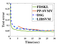
(a) gisette

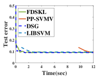
(b) phishing

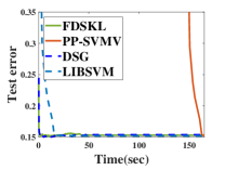
(c) a9a

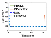
(d) ijcnn1

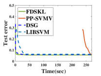
(e) cod-rna

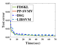
(f) w8a

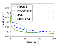
(g) real-sim

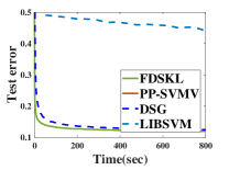
(h) epsilon

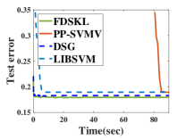
(i) deafultcredit

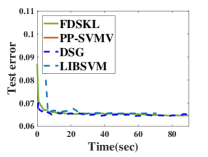
(j) givemecredit

Figure 3: The results of binary classification above the comparison methods.

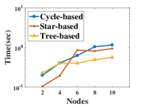
(a) gisette

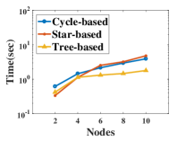
(b) phishing

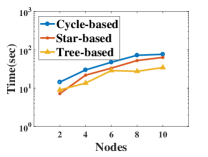
(c) a9a

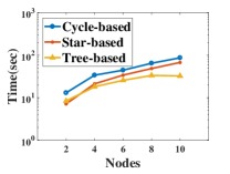
(d) ijcnn1

Figure 4: The elapsed time of different structures on four datasets.

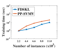
(a) phishing

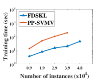
(b) a9a

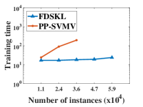
(c) cod-rna

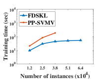
(d) w8a

Figure 5: The change of training time when increasing the number of training instances.

4.2 Results and Discussions

We provide the test errors v.s. training time plot on four state-of-the-art kernel methods in Figure 3. It is evident that our algorithm always achieves fastest convergence rate compared to other state-of-art kernel methods. In Figure 5, we demonstrate the training time v.s. different training sizes of FDSKL and PP-SVMV. Again, the absence of the results in Figures 5(b), 5(c) and 5(d) for PP-SVMV is because of out of memory. It is obvious that our method has much better scalability than PP-SVMV. The reason for this edge of scalability is comprehensive, mostly because FDSKL have adopted the random feature approach, which is efficient and easily parallelizable. Besides, we could also demonstrate that the communication structure used in PP-SVMV is not optimal, which means more time spent in sending and receiving the partitioned kernel matrix.

As mentioned in previous section, FDSKL used a tree-structured communication scheme to distribute and aggregate computation. To verify such a systematic design, we compare the efficiency of 3 commonly used communication structures, i.e., cycle-based, tree-based and star-based communication structures. The goal of the comparison task is to compute the kernel matrix (linear kernel) of the training set of four datasets. Specifically, each node maintains a feature subset of the training set, and is asked to compute the kernel matrix using the feature subset only. The computed local kernel matrices on each node are then summed by using one of the three communication structures. Our experiment compares the efficiency (elapsed communication time) of obtaining the final kernel matrix, and the results are given in Figure 4. From Figure 4, we could make a statement that with the increase of nodes, our tree-based communication structure has the lowest communication cost. This explains the poor efficiency of PP-SVMV, which used a cycle-based communication structure, as given in Figure 5.

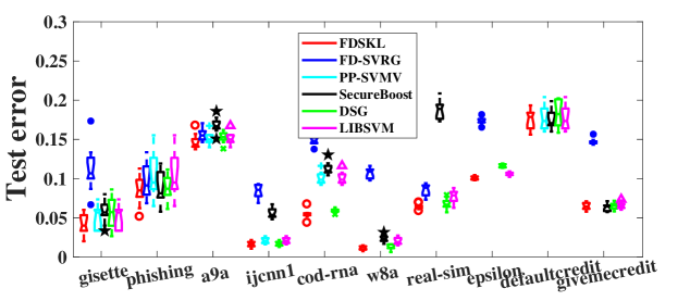
Figure 6: The boxplot of test errors of three state-of-the-art kernel methods, tree-boosting method (SecureBoost), linear method (FD-SVRG) and our FDSKL.

Table 4: The comparison of total training time between our FDSKL and SecureBoost algorithm.

Datasets	FDSKL (min)	SecureBoost (min)
gisette	1	46
phishing	1	10
a9a	2	15
ijcnn1	1	17
cod-rna	1	16
w8a	1	17
real-sim	14	65
epsilon	29	$>$900
defaultcredit	1	13
givemecredit	3	32

Since the official implementation of SecureBoost algorithm did not provide the elapsed time of each iteration, we present the total training time between our FDSKL and SecureBoost in Table 4. From these results, we could make a statement that SecureBoost algorithm is not suitable for the high dimension or large scale datasets which limits its generalization.

Finally, we present the test errors of three state-of-the-art kernel methods, tree-boosting method (SecureBoost), linear method (FD-SVRG) and our FDSKL in Figure 6. All results are averaged over 10 different train-test split trials (Gu and Ling, 2015). From the results, we find that our FDSKL always has the lowest test error and variance. In addition, tree-boosting method SecureBoost performs poor in high-dimensional datasets such as real-sim. And the linear method normally has worse results than other kernel methods.

5 Conclusion

Privacy-preservation federated learning for vertically partitioned data is urgent currently in data mining and machine learning. In this paper, we proposed a federated doubly stochastic kernel learning (i.e., FDSKL) algorithm for vertically partitioned data, which breaks the limitation of implicitly linear separability used in the existing privacy-preservation federated learning algorithms. We proved that FDSKL has a sublinear convergence rate, and can guarantee data security under the semi-honest assumption. To the best of our knowledge, FDSKL is the first efficient and scalable privacy-preservation federated kernel method. Extensive experimental results show that FDSKL is more efficient than the existing state-of-the-art kernel methods for high dimensional data while retaining the similar generalization performance.

Appendix A: Proof of Theorem 4

We first prove that the output of Algorithm 3 is actually $\omega_{i}^{T}x+b$ in Lemma 1 which is the basis of FDSKL.

Lemma 1

The output of Algorithm 3 (i.e., $\sum_{\hat{\ell}=1}^{q}\left((\omega_{i})_{\mathcal{G}_{\hat{\ell}}}^{T}(x)_{\mathcal{G}_{\hat{\ell}}}+b^{\hat{\ell}}\right)-\overline{b}^{\ell^{\prime}}$ is equal to $\omega_{i}^{T}x+b$, where each $b^{\hat{\ell}}$ and $b$ are drawn from a uniform distribution on $[0,2\pi]$, $\overline{b}^{\ell^{\prime}}=\sum_{{\hat{\ell}}\neq\ell^{\prime}}b^{{\hat{\ell}}}$, and $\ell^{\prime}\in\{1,\ldots,q\}-\{\ell\}$.

Proof  The proof has two parts: 1) Because each worker knows the same probability measure $\mathbb{P}(\omega)$, and has a same random seed $i$, each worker can generate the same random feature $\omega$ according to the same random seed $i$. Thus, we can locally compute $(\omega_{i})_{\mathcal{G}_{\ell}}^{T}(x)_{\mathcal{G}_{\ell}}$, and get $\sum_{\ell=1}^{q}(\omega_{i})_{\mathcal{G}_{\ell}}^{T}(x)_{\mathcal{G}_{\ell}}=\omega_{i}^{T}x$. 2) Because each $b^{\hat{\ell}}$ is drawn from a uniform distribution on $[0,2\pi]$, we can have that $\sum_{\hat{\ell}=1}^{q}b^{\hat{\ell}}-\overline{b}^{\ell^{\prime}}=\sum_{\ell=1}^{q}b^{\hat{\ell}}-\sum_{\hat{\ell}\neq\ell^{\prime}}b^{{\hat{\ell}}}$ is also drawn from a uniform distribution on $[0,2\pi]$. This completes the proof.  

Based on Lemma 1, we can conclude that the federated learning algorithm (i.e., FDSKL) can produce the doubly stochastic gradients exactly same to the ones of DSG algorithm with constant learning rate. Thus, under Assumption 1, we can prove that FDSKL converges to the optimal solution almost at a rate of $\mathcal{O}(1/t)$ as shown in Theorem 4.

Now we will show that Algorithm 1 with constant stepsize is convergent in terms of $||f-f_{*}||^{2}_{\cal H}$ with a rate of near $O(1/t)$, where $f^{*}$ is the minimizer of problem. And then we decompose the error according to its sources, which include the error from random features $|f_{t}(x)-h_{t}(x)|^{2}$, and the error from data randomness $||h_{t}(x)-f_{*}(x)||^{2}_{\cal H}$, that is:

$$|f_{t}(x)-f_{*}(x)|^{2}\leq 2|f_{t}(x)-h_{t}(x)|^{2}+2\kappa||h_{t}-f_{*}||_{\cal H}^{2}$$ (9)

Before we show the main Theorem 2, we first give several following lemmas. Note that, different from the proof of (Dai et al., 2014), we obtain the Lemma 3 by the summation formula of geometric progression and the Lemma 4 inspired by the proof of the recursive formula in (Recht et al., 2011). Firstly, we give the convergence analysis of error due to random feature. Let $\mathcal{D}_{t}$ denote the subset of $\mathcal{S}$ which have been picked up at the $t$-th iteration of FDSKL.

Lemma 3

For any $x\in\cal X$ and $\frac{1}{\lambda}>\gamma>0$,

$$\mathbb{E}_{{\cal D}_{t},\omega_{t}}\Big{[}\Big{|}f_{t+1}(x)-h_{t+1}(x)\Big{|}^{2}\Big{]}\leq C^{2}$$ (10)

where $C^{2}:=M^{2}(\sqrt{\kappa}+\sqrt{\phi})^{2}\gamma/\lambda$.

Proof  We denote $W_{i}(x)=W_{i}(x;\mathcal{D}^{i},\omega^{i}):=\alpha^{t}_{i}(\zeta_{i}(x)-\xi_{i}(x))$. According to the above assumptions, $W_{i}(x)$ have a bound:

$$|W_{i}(x)|\leq c_{i}=|\alpha^{t}_{i}|(|\zeta_{i}(x)|+|\xi_{i}(x)|)=M(\sqrt{\kappa}+\sqrt{\phi})|\alpha^{t}_{i}|$$

Obviously, $|\alpha^{t}_{t}|\leq\gamma$, and $|\alpha^{t}_{i}|\leq\gamma\prod^{t}_{j=i+1}(1-\gamma c)\leq\gamma$ where $(1-\gamma\lambda)\leq 1$. Considering the summation formula of geometric progression, $\sum_{i=1}^{t}|\alpha^{t}_{i}|\leq\frac{1}{\lambda}$. Consequently, $\sum_{i=1}^{t}|\alpha^{t}_{i}|^{2}\leq\frac{\gamma}{\lambda}$.

Then we have: $\mathbb{E}_{{\cal D}_{t},\omega_{t}}\Big{[}\Big{|}f_{t+1}(x)-h_{t+1}(x)\Big{|}^{2}\Big{]}=\sum_{i=1}^{t}|W_{i}(x)|^{2}\leq M^{2}(\sqrt{\kappa}+\sqrt{\phi})^{2}\sum_{i=1}^{t}|\alpha^{t}_{i}|^{2}\leq M^{2}(\sqrt{\kappa}+\sqrt{\phi})^{2}\gamma/\lambda$.

we obtain the above lemma.  

The next lemma gives the convergence analysis of error due to random data, whose derivation actually depends on the results of the previous lemmas.

Lemma 4

Set $\frac{1}{\lambda}>\gamma>0$, with $\gamma=\frac{\epsilon\vartheta}{2B}$ for $\vartheta\in\left(\right.0,1\left.\right]$, we will reach $\mathbb{E}\Big{[}||h_{t}-f_{*}||_{\cal H}^{2}\Big{]}\leq\epsilon$ after

$$t\geq\frac{2B\log(2e_{1}/\epsilon)}{\vartheta\epsilon\lambda}$$ (11)

iterations, where $B=\left[\sqrt{G_{2}^{2}+G_{1}}+G_{2}\right]^{2}$, $G_{1}=\frac{2\kappa M^{2}}{\lambda}$, $G_{2}=\frac{\kappa^{1/2}M(\sqrt{\kappa}+\sqrt{\phi})}{2\lambda^{3/2}}$ and $e_{1}=\mathbb{E}[\|h_{1}-f_{*}\|_{\mathcal{H}}^{2}]$.

Proof  In order to simplify the notations, let us denote the following three different gradient terms, they are:

$$g_{t}=\xi_{t}+ch_{t}=L_{t}^{\prime}(f_{t})k(x_{t},\cdot)+\lambda h_{t}$$

$$\hat{g}_{t}=\hat{\xi_{t}}+\lambda h_{t}=L_{t}^{\prime}(h_{t})k(x_{t},\cdot)+\lambda h_{t}$$

$$\bar{g}_{t}=\mathbb{E}_{{\cal D}_{t}}[\hat{g}_{t}]=\mathbb{E}_{{\cal D}_{t}}[L_{t}^{\prime}(h_{t})k(x_{t},\cdot)]+\lambda h_{t}$$

From previous definition, we have $h_{t+1}=h_{t}-\gamma g_{t},\forall t\geq 1$.

We denote $A_{t}=\|h_{t}-f_{*}\|_{\mathcal{H}}^{2}$, then we have

$$A_{t+1} =\|h_{t}-f_{*}-\gamma g_{t}\|_{\mathcal{H}}^{2}$$

$$=A_{t}+\gamma^{2}\|g_{t}\|_{\mathcal{H}}^{2}-2\gamma\langle h_{t}-f_{*},g_{t}\rangle_{\mathcal{H}}$$

$$=A_{t}+\gamma^{2}\|g_{t}\|-2\gamma\langle h_{t}-f_{*},\bar{g}_{t}\rangle_{\mathcal{H}}+2\gamma\langle h_{t}-f_{*},\bar{g}_{t}-\hat{g}_{t}\rangle_{\mathcal{H}}+2\gamma\langle h_{t}-f_{*},\hat{g}_{t}-g_{t}\rangle_{\mathcal{H}}$$

Cause the strongly convexity of objective and optimality condition, we have

$$\langle h_{t}-f_{*},\bar{g}_{t}\rangle_{\mathcal{H}}\geq\lambda\|h_{t}-f_{*}\|_{\mathcal{H}}^{2}$$

Hence, we have

$$A_{t+1}\leq(1-2\gamma\lambda)A_{t}+\gamma^{2}\|g_{t}\|_{\mathcal{H}}^{2}+2\gamma\langle h_{t}-f_{*},\bar{g}_{t}-\hat{g}_{t}\rangle_{\mathcal{H}}+2\gamma\langle h_{t}-f_{*},\hat{g}_{t}-g_{t}\rangle_{\mathcal{H}},\forall t\geq 1$$ (12)

Let us denote $\mathcal{M}_{t}=\|g_{t}\|_{\mathcal{H}}^{2},\mathcal{N}_{t}=\langle h_{t}-f_{*},\bar{g}_{t}-\hat{g}_{t}\rangle_{\mathcal{H}},\mathcal{R}_{t}=\langle h_{t}-f_{*},\hat{g}_{t}-g_{t}\rangle_{\mathcal{H}}$. According to Lemma 3, $\mathcal{M}_{t},\mathcal{N}_{t},\mathcal{R}_{t}$ can be bounded. Then we denote $e_{t}=\mathbb{E}_{{\cal D}_{t},\omega_{t}}[A_{t}]$, given the above bounds, we obtain the following recursion,

$$e_{t+1}\leq(1-2\gamma\lambda)e_{t}+4\kappa M^{2}\gamma^{2}+2\kappa^{1/2}L\gamma C\sqrt{e_{t}}$$ (13)

When $\gamma>0$ and $|a_{t}^{i}|\leq\gamma,\forall 1\leq i\leq t$. Consequently, $C^{2}\leq M^{2}(\sqrt{\kappa}+\sqrt{\phi})^{2}\gamma/\lambda$. Applying these bounds to the above recursion, we have

$$e_{t+1}\leq\beta_{1}e_{t}+\beta_{2}+\beta_{3}\sqrt{e_{t}},$$ (14)

Note that $\beta_{1}=1-2\gamma\lambda$, $\beta_{2}=4\kappa M^{2}\gamma^{2}$ and $\beta_{3}=\frac{2\kappa^{1/2}\gamma^{3/2}LM(\sqrt{\kappa}+\sqrt{\phi})}{\sqrt{\lambda}}$. Then consider that when $t\rightarrow\infty$ we have:

$$e_{\infty}=\beta_{1}e_{\infty}+\beta_{2}+\beta_{3}\sqrt{e_{\infty}}$$ (15)

and the solution of the above recursion (15) is

$$e_{\infty}=\left[\sqrt{\frac{\beta_{3}^{2}}{16\gamma^{2}\lambda^{2}}+\frac{\beta_{2}}{2\gamma\lambda}}+\frac{\beta_{3}}{4\gamma\lambda}\right]^{2}=\gamma*\left[\sqrt{G_{2}^{2}+G_{1}}+G_{2}\right]^{2}$$ (16)

where $G_{1}=\frac{2\kappa M^{2}}{\lambda}$ and $G_{2}=\frac{\kappa^{1/2}M(\sqrt{\kappa}+\sqrt{\phi})}{2\lambda^{3/2}}$.

We use Eq. (14) minus Eq. (15), then we get:

$$e_{t+1} \leq\beta_{1}(e_{t}-e_{\infty})+\beta_{3}(\sqrt{e_{t}}-\sqrt{e_{\infty}})+e_{\infty}$$

$$\leq\beta_{1}(e_{t}-e_{\infty})+\beta_{3}(\frac{e_{t}-e_{\infty}}{2\sqrt{e_{\infty}}})+e_{\infty}$$

$$\leq(\beta_{1}+\frac{\beta_{3}}{2\sqrt{e_{\infty}}})(e_{t}-e_{\infty})+e_{\infty}$$

$$\leq(1-\gamma\lambda)(e_{t}-e_{\infty})+e_{\infty}$$ (17)

where the second inequality is due to $a-b\leq\frac{a^{2}-b^{2}}{2b}$, and the last step is due to $\frac{\beta_{3}}{2\sqrt{e_{\infty}}}=\frac{1}{2\left[\sqrt{\frac{1}{16\gamma^{2}\lambda^{2}}+\frac{\beta_{2}}{2\gamma\lambda\beta_{3}^{2}}}+\frac{1}{4\gamma\lambda}\right]}\leq\frac{1}{2[\frac{1}{4\gamma\lambda}+\frac{1}{4\gamma\lambda}]}=\gamma\lambda$.

We can easily apply Eq. (5.1) in (Recht et al., 2011) to Eq. (17), and Eq. (16) satisfy $a_{\infty}(\gamma)\leq\gamma B$. We denote $B=\left[\sqrt{G_{2}^{2}+G_{1}}+G_{2}\right]^{2}$. Particularly, unwrapping (17) we have:

$$e_{t+1}\leq(1-\gamma\lambda)^{t}(e_{1}-e_{\infty})+e_{\infty}$$ (18)

Suppose we want this quantity (18) to be less than $\epsilon$. Similarly, we let both terms are less than $\epsilon/2$, then for the second term, we have

$$\gamma\leq\frac{\epsilon}{2B}=\frac{\epsilon}{2\left[\sqrt{G_{2}^{2}+G_{1}}+G_{2}\right]^{2}}$$ (19)

For the first term, we need:

$$(1-\gamma\lambda)^{t}e_{1}\leq\frac{\epsilon}{2}$$

which holds if

$$t\geq\frac{\log(2e_{1}/\epsilon)}{\gamma\lambda}$$ (20)

According to the (19), we should pick $\gamma=\frac{\epsilon\vartheta}{2B}$ for $\vartheta\in\left(\right.0,1\left.\right]$. Combining this with Eq. (20), after

$$t\geq\frac{2B\log(2e_{1}/\epsilon)}{\vartheta\epsilon\lambda}$$ (21)

iterations we will have $e_{t}\leq\epsilon$ and that give us a $\mathcal{O}(1/t)$ convergence rate, if eliminating the $\log(1/\epsilon)$ factor.

 
Now we give the technical lemma which is used in proving Lemma 5.

Lemma 5

$$\mathcal{M}_{t}\leq 4\kappa M^{2};$$ (22)

$$\mathbb{E}_{{\cal D}_{t},\omega_{t}}\Big{[}{\cal N}_{t}\Big{]}=0$$ (23)

$$\mathbb{E}_{{\cal D}_{t},\omega_{t}}\Big{[}{\cal R}_{t}\Big{]}\leq\kappa^{1/2}\mathcal{L}C\sqrt{\mathbb{E}_{{\cal D}_{t-1},\omega_{t-1}}[A_{t}]}$$ (24)

where $A_{t}=||h_{t}-f_{*}||^{2}_{\cal H}$.

Proof  Firstly, let we prove the Lemma 5.1 (22):

$$\mathcal{M}_{t}=\|g_{t}\|_{\mathcal{H}}^{2}=\|\xi_{t}+\lambda h_{t}\|_{\mathcal{H}}^{2}\leq\left(\|\xi_{t}\|_{\mathcal{H}}+\lambda\|h_{t}\|_{\mathcal{H}}\right)^{2}$$

and

$$\|\xi_{t}\|_{\mathcal{H}}=\|L^{\prime}(f_{t}(x_{t}),y_{t})k(x_{t},\cdot)\|_{\mathcal{H}}\leq\kappa^{1/2}M$$

Then we have:

$$\|h_{t}\|_{\mathcal{H}}^{2} =\sum_{i=1}^{t-1}\sum_{j=1}^{t-1}\alpha^{t-1}_{i}\alpha^{t-1}_{j}L^{\prime}(f_{i}(x_{i}),y_{i})L^{\prime}(f_{j}(x_{j}),y_{j})k(x_{i},x_{j})$$

$$\leq\kappa M^{2}\sum_{i=1}^{t-1}\sum_{j=1}^{t-1}|\alpha^{t-1}_{i}||\alpha^{t-1}_{j}|$$

Consequently, $\|h_{t}\|_{\mathcal{H}}\leq\kappa^{1/2}M\sqrt{\sum_{i,j=1}^{t-1}|\alpha^{t-1}_{i}||\alpha^{t-1}_{j}|}\leq\kappa^{1/2}M\frac{1}{\lambda}$. Then the above equation can be rewritten as:

$$\mathcal{M}_{t}=\|g_{t}\|_{\mathcal{H}}^{2}=\|\xi_{t}+\lambda h_{t}\|_{\mathcal{H}}^{2}\leq\left(\|\xi_{t}\|_{\mathcal{H}}+\lambda\|h_{t}\|_{\mathcal{H}}\right)^{2}\leq(\kappa^{1/2}M+\lambda\times\kappa^{1/2}M\frac{1}{\lambda})^{2}=4\kappa M^{2}5$$

Therefore, we finish the proof of Lemma 5.1.

For the second one (23), ${\cal N}_{t}=\langle h_{t}-f_{*},\bar{g}_{t}-\hat{g}_{t}\rangle_{\mathcal{H}}$, then we have:

$$\mathbb{E}_{{\cal D}_{t},\omega_{t}}\Big{[}{\cal N}_{t}\Big{]} =\mathbb{E}_{{\cal D}_{t-1},\omega_{t}}\left[\mathbb{E}_{{\cal D}_{t-1}}[\langle h_{t}-f_{*},\bar{g}_{t}-\hat{g}_{t}\rangle_{\mathcal{H}}|{\cal D}_{t-1},\omega_{t}]\right]$$

$$=\mathbb{E}_{{\cal D}_{t-1},\omega_{t}}\left[\langle h_{t}-f_{*},\mathbb{E}_{{\cal D}_{t}}[\bar{g}_{t}-\hat{g}_{t}]\rangle_{\mathcal{H}}\right]$$

$$=0$$

The third one (24), ${\cal R}_{t}=\langle h_{t}-f_{*},\hat{g}_{t}-g_{t}\rangle_{\mathcal{H}}$, then we have:

$$\mathbb{E}_{{\cal D}_{t},\omega_{t}}\Big{[}{\cal R}_{t}\Big{]} =\mathbb{E}_{{\cal D}_{t},\omega_{t}}\Big{[}\langle h_{t}-f_{*},\hat{g}_{t}-g_{t}\rangle_{\mathcal{H}}\Big{]}$$

$$=\mathbb{E}_{{\cal D}_{t},\omega_{t}}\Big{[}\langle h_{t}-f_{*},[l^{\prime}(f_{t}(x_{t}),y_{t})-l^{\prime}(h_{t}(x_{t}),y_{t})]k(x_{t},\cdot)\rangle_{\mathcal{H}}\Big{]}$$

$$\leq\mathbb{E}_{{\cal D}_{t},\omega_{t}}\Big{[}\|h_{t}-f_{*}\|_{\mathcal{H}}\cdot|l^{\prime}(f_{t}(x_{t}),y_{t})-l^{\prime}(h_{t}(x_{t}),y_{t})|\cdot\|k(x_{t},\cdot)\|_{\mathcal{H}}\Big{]}$$

$$\leq\kappa^{1/2}\mathcal{L}\cdot\mathbb{E}_{{\cal D}_{t},\omega_{t}}\Big{[}\|h_{t}-f_{*}\|_{\mathcal{H}}\cdot|f_{t}(x_{t})-h_{t}(x_{t})|\Big{]}$$

$$\leq\kappa^{1/2}\mathcal{L}\cdot\sqrt{\mathbb{E}_{{\cal D}_{t},\omega_{t}}\|h_{t}-f_{*}\|_{\mathcal{H}}^{2}}\sqrt{\mathbb{E}_{{\cal D}_{t},\omega_{t}}|f_{t}(x_{t})-h_{t}(x_{t})|^{2}}$$

$$\leq\kappa^{1/2}\mathcal{L}\cdot C\sqrt{\mathbb{E}_{{\cal D}_{t-1},\omega_{t-1}}[A_{t}]}$$

where the first and third inequalities are due to Cauchy-Schwarz Inequality and the second inequality is due to the Assumptions 1. And the last step is due to the Lemma 1 and the definition of $A_{t}$.  

According to Lemmas 3 and 4, we obtain the final results on convergence in expectation:

Theorem 2 (Convergence in expectation)

Set $\epsilon>0$, $\min\{\frac{1}{\lambda},\frac{\epsilon\lambda}{4M^{2}(\sqrt{\kappa}+\sqrt{\phi})^{2}}\}>\gamma>0$, for Algorithm 1, with $\gamma=\frac{\epsilon\vartheta}{8\kappa B}$ for $\vartheta\in\left(\right.0,1\left.\right]$, we will reach $\mathbb{E}\Big{[}|f_{t}(x)-f_{*}(x)|^{2}\Big{]}\leq\epsilon$ after

$$t\geq\frac{8\kappa B\log(8\kappa e_{1}/\epsilon)}{\vartheta\epsilon\lambda}$$ (25)

iterations, where $B\text{ and }e_{1}$ are as defined in Lemma 4.

Proof  Substitute Lemma 3 and 4 into the inequality (9), i.e.

$$\mathbb{E}\Big{[}|f_{t}(x)-f_{*}(x)|^{2}\Big{]}$$

$$\leq 2\mathbb{E}\Big{[}|f_{t}(x)-h_{t+1}(x)|^{2}\Big{]}+2\kappa\mathbb{E}\Big{[}||h_{t}-f_{*}||^{2}_{\cal H}\Big{]}$$

$$\leq\epsilon$$

Again, it is sufficient that both terms are less than $\epsilon/2$. For the second term, we can directly derive from Lemma 4. As for the first term, we can get a upper bound of $\gamma$: $\frac{\epsilon\lambda}{4M^{2}(\sqrt{\kappa}+\sqrt{\phi})^{2}}$. Then we obtain the above theorem.

 

Appendix B: Proof of Lemma 2

Lemma 2

Using a tree structure $T_{2}$ for workers $\{1,\ldots,q\}-\{\ell^{\prime}\}$ which is totally different to the tree $T_{1}$ to compute $\overline{b}^{\ell^{\prime}}=\sum_{{\hat{\ell}}\neq\ell^{\prime}}b^{{\hat{\ell}}}$, for any worker, there is no risk to disclose the value of $b^{{{\hat{\ell}}}}$ or the sum of $b^{{{\hat{\ell}}}}$ on other workers.

Proof  If there exist the inference attack, the inference attack must happen in one non-leaf node in the tree $T_{1}$. We denote the non-leaf node as NODE.

Assume the $\ell$-th worker is one of the leafs of the subtree of NODE. If the $\ell$-th worker wants to start the inference attack, it is necessary to have the sum of all $b^{\ell^{\prime}}$ on the leaves of the tree, which means that the subtree corresponding to NODE also belongs to $T_{2}$.  

Appendix C: Complexity Analysis of FDSKL

We derive the computational complexity and communication cost of FDSKL as follows.

1. The line 2 of Algorithm 1 picks up an instance $(x_{i})_{\mathcal{G}_{\ell}}$ from the local data $D^{\ell}$ with index $i$. Thus, its computational complexity of all workers is $\mathcal{O}(q)$, and there is no communication cost.

2. The line 3 of Algorithm 1 sends $i$ to other workers using a reverse-order tree structure. Thus, its computational complexity is $\mathcal{O}(1)$, and the communication cost is $\mathcal{O}(q)$.

3. The line 4 of Algorithm 1 samples $\omega_{i}\sim\mathbb{P}(\omega)$ with the random seed $i$. Thus, its computational complexity of all workers is $\mathcal{O}(dq)$, and there is no communication cost.

4. The line 5 of Algorithm 1 computes $\omega_{i}^{T}x_{i}+b$. The detailed procedure is presented in Algorithm 3. Its computational complexity is $\mathcal{O}(d+q)$, and the communication cost is $\mathcal{O}(q)$. The detailed analysis of computational complexity and communication cost of Algorithm 3 is omitted here.

5. The lines 6-7 of Algorithm 1 uses the tree-structured communication scheme to compute $f(x_{i})=\sum_{\ell=1}^{q}f^{\ell}(x_{i})$. Because the computational complexity and communication cost of $f^{\ell}(x)$ are $\mathcal{O}(dq|\Lambda^{\ell}|)$ and $\mathcal{O}(q|\Lambda^{\ell}|)$, respectively, as analyzed in the next part, we can conclude that the computational complexity of lines 6-7 of Algorithm 1 is $\mathcal{O}(dqt)$, and its communication cost is $\mathcal{O}(qt)$, where $t$ is the global iteration number.

6. The line 8-9 of Algorithm 1 compute the current coefficient $\alpha_{i}$. Thus, its computational complexity is $\mathcal{O}(1)$, and there is no communication cost.

7. The line 10 of Algorithm 1 updates the former coefficients. Thus, its computational complexity of all workers is $\mathcal{O}(t)$, and its communication cost is $\mathcal{O}(q)$.

Based on the above discussion, the computational complexity for one iteration of FDSKL is $\mathcal{O}(dqt)$. Thus, the total computational complexity of FDSKL is $\mathcal{O}(dqt^{2})$. Further, the communication cost for one iteration of FDSKL is $\mathcal{O}(qt)$, and the total communication cost of FDSKL is $\mathcal{O}(qt^{2})$.

We derive the computational complexity and communication cost of Algorithm 2 as follows.

1. The line 1 of Algorithm 2 sets the initial solution to $f^{\ell}(x)$. Thus, its computational complexity is $\mathcal{O}(1)$, and there is no communication cost.

2. The lines 3-5 of Algorithm 2 compute $\phi_{\omega_{i}}(x)$ which are similar to the lines 4-5 of Algorithm 1. According to the previous analyses in this section, we have that its computational complexity is $\mathcal{O}(dq)$, and the communication cost is $\mathcal{O}(q)$.

3. The line 6 of Algorithm 2 is updating the value of $f^{\ell}(x)$. Thus, its computational complexity is $\mathcal{O}(1)$, and there is no communication cost.

Thus, the computational complexity of Algorithm 2 is $\mathcal{O}(dq|\Lambda^{\ell}|)$ and the communication cost of Algorithm 2 is $\mathcal{O}(q|\Lambda^{\ell}|)$.

References

- Badshah (2018) Nadeem Badshah. Facebook to contact 87 million users affected by data breach. The Guardian) Retrieved from https://www. theguardian. com/technology/2018/apr/08/facebook-to-contact-the-87-million-users-affected-by-data-breach, 2018.
- Berlinet and Thomas-Agnan (2011) Alain Berlinet and Christine Thomas-Agnan. Reproducing kernel Hilbert spaces in probability and statistics. Springer Science & Business Media, 2011.
- Chang and Lin (2011) Chih-Chung Chang and Chih-Jen Lin. LIBSVM: A library for support vector machines. ACM Transactions on Intelligent Systems and Technology, 2:1–27, 2011. Software available at http://www.csie.ntu.edu.tw/~cjlin/libsvm.
- Cheng et al. (2019) Kewei Cheng, Tao Fan, Yilun Jin, Yang Liu, Tianjian Chen, and Qiang Yang. Secureboost: A lossless federated learning framework. arXiv preprint arXiv:1901.08755, 2019.
- Dai et al. (2014) Bo Dai, Bo Xie, Niao He, Yingyu Liang, Anant Raj, Maria-Florina F Balcan, and Le Song. Scalable kernel methods via doubly stochastic gradients. In Advances in Neural Information Processing Systems, pages 3041–3049, 2014.
- Dalcin et al. (2011) Lisandro D Dalcin, Rodrigo R Paz, Pablo A Kler, and Alejandro Cosimo. Parallel distributed computing using python. Advances in Water Resources, 34(9):1124–1139, 2011.
- Du and Atallah (2001) Wenliang Du and Mikhail J Atallah. Privacy-preserving cooperative statistical analysis. In Seventeenth Annual Computer Security Applications Conference, pages 102–110. IEEE, 2001.
- EU (2016) EU. Regulation (eu) 2016/679 of the european parliament and of the council on the protection of natural persons with regard to the processing of personal data and on the free movement of such data, and repealing directive 95/46/ec (general data protection regulation). Available at https://eur-lex.europa.eu/legal-content/EN/TXT, 2016.
- Gascón et al. (2016) Adrià Gascón, Phillipp Schoppmann, Borja Balle, Mariana Raykova, Jack Doerner, Samee Zahur, and David Evans. Secure linear regression on vertically partitioned datasets. IACR Cryptology ePrint Archive, 2016:892, 2016.
- Gascón et al. (2017) Adrià Gascón, Phillipp Schoppmann, Borja Balle, Mariana Raykova, Jack Doerner, Samee Zahur, and David Evans. Privacy-preserving distributed linear regression on high-dimensional data. Proceedings on Privacy Enhancing Technologies, 2017(4):345–364, 2017.
- Geng et al. (2019) Xiang Geng, Bin Gu, Xiang Li, Wanli Shi, Guansheng Zheng, and Heng Huang. Scalable semi-supervised svm via triply stochastic gradients. In Proceedings of the 28th International Joint Conference on Artificial Intelligence, pages 2364–2370. AAAI Press, 2019.
- Gu and Ling (2015) Bin Gu and Charles Ling. A new generalized error path algorithm for model selection. In International Conference on Machine Learning, pages 2549–2558, 2015.
- Gu et al. (2008) Bin Gu, Jiandong Wang, and Haiyan Chen. On-line off-line ranking support vector machine and analysis. In 2008 IEEE International Joint Conference on Neural Networks (IEEE World Congress on Computational Intelligence), pages 1364–1369. IEEE, 2008.
- Gu et al. (2018a) Bin Gu, Zhouyuan Huo, and Heng Huang. Asynchronous doubly stochastic group regularized learning. In International Conference on Artificial Intelligence and Statistics, pages 1791–1800, 2018a.
- Gu et al. (2018b) Bin Gu, Yingying Shan, Xiang Geng, and Guansheng Zheng. Accelerated asynchronous greedy coordinate descent algorithm for svms. In IJCAI, pages 2170–2176, 2018b.
- Gu et al. (2018c) Bin Gu, Miao Xin, Zhouyuan Huo, and Heng Huang. Asynchronous doubly stochastic sparse kernel learning. In Thirty-Second AAAI Conference on Artificial Intelligence, 2018c.
- Gu et al. (2018d) Bin Gu, Xiao-Tong Yuan, Songcan Chen, and Heng Huang. New incremental learning algorithm for semi-supervised support vector machine. In Proceedings of the 24th ACM SIGKDD International Conference on Knowledge Discovery & Data Mining, pages 1475–1484, 2018d.
- Gu et al. (2019) Bin Gu, Zhouyuan Huo, and Heng Huang. Scalable and efficient pairwise learning to achieve statistical accuracy. In Proceedings of the AAAI Conference on Artificial Intelligence, volume 33, pages 3697–3704, 2019.
- Hardy et al. (2017) Stephen Hardy, Wilko Henecka, Hamish Ivey-Law, Richard Nock, Giorgio Patrini, Guillaume Smith, and Brian Thorne. Private federated learning on vertically partitioned data via entity resolution and additively homomorphic encryption. arXiv preprint arXiv:1711.10677, 2017.
- Karr et al. (2009) Alan F Karr, Xiaodong Lin, Ashish P Sanil, and Jerome P Reiter. Privacy-preserving analysis of vertically partitioned data using secure matrix products. Journal of Official Statistics, 25(1):125, 2009.
- Liu et al. (2019) Yang Liu, Yingting Liu, Zhijie Liu, Junbo Zhang, Chuishi Meng, and Yu Zheng. Federated forest. arXiv preprint arXiv:1905.10053, 2019.
- Nock et al. (2018) Richard Nock, Stephen Hardy, Wilko Henecka, Hamish Ivey-Law, Giorgio Patrini, Guillaume Smith, and Brian Thorne. Entity resolution and federated learning get a federated resolution. arXiv preprint arXiv:1803.04035, 2018.
- Rahimi and Recht (2008) Ali Rahimi and Benjamin Recht. Random features for large-scale kernel machines. In Advances in neural information processing systems, pages 1177–1184, 2008.
- Rahimi and Recht (2009) Ali Rahimi and Benjamin Recht. Weighted sums of random kitchen sinks: Replacing minimization with randomization in learning. In Advances in neural information processing systems, pages 1313–1320, 2009.
- Recht et al. (2011) Benjamin Recht, Christopher Re, Stephen Wright, and Feng Niu. Hogwild: A lock-free approach to parallelizing stochastic gradient descent. In Advances in neural information processing systems, pages 693–701, 2011.
- Rudin (1962) Walter Rudin. Fourier analysis on groups, volume 121967. Wiley Online Library, 1962.
- Sanil et al. (2004) Ashish P Sanil, Alan F Karr, Xiaodong Lin, and Jerome P Reiter. Privacy preserving regression modelling via distributed computation. In Proceedings of the tenth ACM SIGKDD international conference on Knowledge discovery and data mining, pages 677–682. ACM, 2004.
- Shi et al. (2019) Wanli Shi, Bin Gu, Xiang Li, Xiang Geng, and Heng Huang. Quadruply stochastic gradients for large scale nonlinear semi-supervised auc optimization. In Proceedings of the 28th International Joint Conference on Artificial Intelligence, pages 3418–3424. AAAI Press, 2019.
- Shi et al. (2020) Wanli Shi, Bin Gu, Xiang Li, and Heng Huang. Quadruply stochastic gradient method for large scale nonlinear semi-supervised ordinal regression AUC optimization. In The Thirty-Fourth AAAI Conference on Artificial Intelligence, New York, NY, USA, February 7-12, 2020, pages 5734–5741. AAAI Press, 2020.
- Skillicorn and Mcconnell (2008) D. B. Skillicorn and S. M. Mcconnell. Distributed prediction from vertically partitioned data. Journal of Parallel & Distributed Computing, 68(1):16–36, 2008.
- Vaidya and Clifton (2002) Jaideep Vaidya and Chris Clifton. Privacy preserving association rule mining in vertically partitioned data. In Proceedings of the eighth ACM SIGKDD international conference on Knowledge discovery and data mining, pages 639–644. ACM, 2002.
- Vaidya and Clifton (2003) Jaideep Vaidya and Chris Clifton. Privacy-preserving k-means clustering over vertically partitioned data. In Proceedings of the ninth ACM SIGKDD international conference on Knowledge discovery and data mining, pages 206–215, 2003.
- Wan et al. (2007) Li Wan, Wee Keong Ng, Shuguo Han, and Vincent Lee. Privacy-preservation for gradient descent methods. In Proceedings of the 13th ACM SIGKDD international conference on Knowledge discovery and data mining, pages 775–783. ACM, 2007.
- Xie et al. (2015) Bo Xie, Yingyu Liang, and Le Song. Scale up nonlinear component analysis with doubly stochastic gradients. In Advances in Neural Information Processing Systems, pages 2341–2349, 2015.
- Yang et al. (2014) Jiyan Yang, Vikas Sindhwani, Quanfu Fan, Haim Avron, and Michael W Mahoney. Random laplace feature maps for semigroup kernels on histograms. In Proceedings of the IEEE Conference on Computer Vision and Pattern Recognition, pages 971–978, 2014.
- Yu et al. (2006) Hwanjo Yu, Jaideep Vaidya, and Xiaoqian Jiang. Privacy-preserving svm classification on vertically partitioned data. In Pacific-Asia Conference on Knowledge Discovery and Data Mining, pages 647–656. Springer, 2006.
- Zhang et al. (2018) Gong-Duo Zhang, Shen-Yi Zhao, Hao Gao, and Wu-Jun Li. Feature-distributed svrg for high-dimensional linear classification. arXiv preprint arXiv:1802.03604, 2018.
- Zhang et al. (2009) Haizhang Zhang, Yuesheng Xu, and Jun Zhang. Reproducing kernel banach spaces for machine learning. Journal of Machine Learning Research, 10(Dec):2741–2775, 2009.