Limitation of symmetry breaking by gravitational collapse: the revisit of Lin-Mestel-Shu instability

Abstract

We revisit the topic of shape evolution during the spherical collapse of an $N$-body system. Our main objective is to investigate the critical particle number below which, during a gravitational collapse, the amplification of triaxiality from initial fluctuations is effective, and above which it is ineffective. To this aim, we develop the Lin-Mestel-Shu theory for a system of particles initially with isotropic velocity dispersion and with a simple power-law density profile. We first determine, for an unstable cloud, two radii corresponding to the balance of two opposing forces and their fluctuations: such radii fix the sizes of the non-collapsing region and the triaxial seed from density fluctuations. We hypothesize that the triaxial degree of the final state depends on which radius is dominant prior to the collapse phase leading to a different scheme of the self-consistent shape evolution of the core and the rest of the system. The condition where the two radii are equal therefore identifies the critical particle number, which can be expressed as the function of the parameters of initial state. In numerical work, we can pinpoint such a critical number by comparing the virialized flattening with the initial flattening. The difference between these two quantities agrees with the theoretical predictions only for the power-law density profiles with an exponent in the range $[0,0.25]$. For higher exponents, results suggest that the critical number is above the range of simulated $N$. We speculate that there is an additional mechanism, related to strong density gradients that increases further the flattening, requiring higher $N$ to further weaken the initial fluctuations.

1 Introduction

The gravitational collapse model is widely considered to be a potential explanation for the origin and early behavior of elliptical galaxies. The Lin-Mestel-Shu (LMS) theory represents a well-established framework for this model (Lin, Mestel & Shu, 1965). The numerical solutions of the self-consistent equations of motion explain that, in a collapse starting from rest, both unstable prolate and unstable oblate ellipsoids can enhance their flattening. From a dynamical point of view, the relaxation mechanism for out-of-equilibrium systems, known as violent relaxation theory, was provided by Lynden-Bell (1967). It aims, at first, to resolve the mystery of light distribution of elliptical galaxies, which appears to conform with the universal de Vaucouleurs’ profile (de Vaucouleurs, 1953), and to address the problem of their formation time-scale, which appears to be longer than the age of the universe. This mechanism drives the system to an unthermalized quasi-stationary state (QSS) that depends on the initial conditions within a time-scale comparable to the dynamical time. Early tests of these hypotheses by Aarseth & Binney (1978), in which the initial systems were unstable flat ellipsoids, have shown the formation of relaxed structures with a wide range of ellipticity and other properties. Then, the series of gravitational collapses with diversified initial conditions have demonstrated that the final state may have ellipticity up to E4 (van Albada, 1982; McGlynn, 1984).

In the following years, various systematic studies have allowed us to better understand the dependences on some initial system parameters such as the rotational speed (Aguilar & Merritt, 1990), the virial ratio (Theis & Spurzem, 1999; Roy & Perez, 2004), the power-law index of the density profile (Cannizzo & Hollister, 1992; Boily & Athanassoula, 2006; Sylos Labini et al., 2015), or the velocity anisotropy (Barnes et al., 2009). By choosing the velocity dispersion of the initial state as free parameter, then a compilation of past results suggests that one can roughly classify the relaxation mechanism as leading to strong or weak symmetry breaking. Systems that relax starting from a low supporting pressure tend to strongly break the initial symmetry while systems initially possessing a high velocity dispersion tend to remain close to this symmetry. Some studies are able to partition the strong and weak symmetry breaking regimes using the virial ratio or the velocity anisotropy parameter (Min & Choi, 1989; Aguilar & Merritt, 1990; Boily & Athanassoula, 2006; Barnes et al., 2009). In addition to the difference of the flattening amplification, the relaxed density profile and velocity anisotropy are also found to be different (McGlynn, 1984; Aguilar & Merritt, 1990; Sylos Labini, 2012, 2013).

While the dependences on initial state parameters are commonly studied, effects from finite-$N$ fluctuations that are embedded in the initial conditions have not attracted much attention, although several authors have noticed their role. For instance, this issue has been raised by Aarseth et al. (1988) and then it was revisited by Boily et al. (2002) and Joyce et al. (2009). In particular in this latter work, it was shown that finite-$N$ fluctuations have a key role in the system evolution determining the post-collapse ejection of matter and energy from the system. The effect of Poissonian fluctuations on the final system’s shape has been studied in the works of Roy & Perez (2004) and Boily & Athanassoula (2006), where it was concluded to have a negligible effect provided that the number of system particles $N$ is high enough. That conclusion was revised by Worrakitpoonpon (2015); Benhaiem & Sylos Labini (2015) where it was reported, by making accurate systematic tests, that the flattening and other parameters of the virialized states constantly vary in a wide range of $N$. In addition, Benhaiem et al. (2018) have shown that by reducing the density fluctuations (i.e. increasing $N$), the onset of the radial orbit instability can be turned off. This result emphasizes the significance of statistical density fluctuations in the violent relaxation mechanism.

In this work, we revisit the spherical collapse paradigm, focusing on the morphological evolution of an isolated self-gravitating system of particles toward an ellipsoidal stationary state. Our main purpose is to find the critical particle number separating between effective and ineffective evolution to triaxial shape of an isolated system. We study this problem by making use of an extensive set of $N$-body simulations. Comparing to past studies with a similar purpose, we have enlarged the analysis in several ways. Firstly, we develop the collapse model of an $N$-particle cloud based on the inside-out evolution scenario of the LMS theory by considering the role of fluctuations both in the density and velocity spaces. Secondly, we propose a reliable measurement to differentiate the numerical results that allows us to test our hypothesis.

The article is organized as follows. In Section 2, we describe the initial conditions that we have considered for the numerical evolution. In addition, we present the theoretical model that we develop from the LMS framework. Our analysis finally leads to identifying the critical particle number as a function of system parameters: such an analysis will be then compared with the results of numerical simulations. The technical details of the simulations including the preparation and accuracy control are given in Section 3. In Section 4, we report the numerical results of the shape evolution by violent relaxation and compare them with the theoretical predictions. Finally in Section 5 and 6, we provide respectively the conclusions of our study and some further discussion about how our results relate to past work.

2 Analysis of unstable particle clouds

2.1 Properties of initial conditions

Initial conditions are represented by spherical clouds of particles with a power-law density profile with a cut-off of the type

$$\rho(r)=\frac{(3-\alpha)M}{4\pi r_{0}^{3-\alpha}r^{\alpha}}$$ (1)

where $M$ is the total mass, $0\leq\alpha\leq 3$ is the power-law index and $r_{0}$ is the cut-off radius: the case $\alpha=0$ corresponds to the uniform case. From Eq. (1), we derive integrated mass in a sphere of radius $r$

$$M(r)=\frac{r^{3-\alpha}}{r_{0}^{3-\alpha}}M$$ (2)

and the average density profile

$$\bar{\rho}(r)\equiv\frac{M(r)}{\frac{4}{3}\pi r^{3}}=\frac{3}{3-\alpha}\rho(r).$$ (3)

The binding potential energy of the system is then

$$U_{0}=-\int_{0}^{r_{0}}\frac{GM(r)\rho(r)(4\pi r^{2}dr)}{r}=-\frac{(3-\alpha)GM^{2}}{(5-2\alpha)r_{0}}.$$ (4)

The systems have initially isotropic top-hat velocity distribution that can be written as

$$\theta(v)=\frac{3M}{4\pi v_{0}^{3}}\;\;\mbox{for $v\leq v_{0}$}$$ (5)

where $v_{0}$ is the cut-off velocity. The normalization condition is then $M=\int_{0}^{v_{0}}\theta(v)(4\pi v^{2}dv)$. The corresponding kinetic energy can be calculated to be

$$T_{0}=\frac{1}{2}\int_{0}^{v_{0}}v^{2}\theta(v)(4\pi v^{2}dv)=\frac{3}{10}Mv_{0}^{2}.$$ (6)

The uniform velocity distribution $\theta(v)$ has dispersion $\sigma$ such that

$$\sigma^{2}=\frac{1}{M}\int_{0}^{v_{0}}v^{2}\theta(v)(4\pi v^{2}dv)=\frac{3}{5}v_{0}^{2}.$$ (7)

The pressure due to random motions in a spherical system of radius $r$ is

$$p(r)=\frac{1}{3}\sigma^{2}\rho(r).$$ (8)

Note that for $\alpha=0$, the pressure is uniform as the density. From Eq. (4) and (6), we find that initial virial ratio reads

$$b_{0}\equiv\frac{2T_{0}}{|U_{0}|}=\frac{(5-2\alpha)r_{0}\sigma^{2}}{(3-\alpha)GM}.$$ (9)

2.2 Equilibrium of forces and effects of density fluctuations

Let us firstly consider spherical clouds with $\alpha>0$. The inward gravitational force per unit mass at any radius is

$$f_{g}(r)=\frac{GM(r)}{r^{2}}=\frac{GMr^{1-\alpha}}{r_{0}^{3-\alpha}}.$$ (10)

The outward pressure force per unit mass can also be calculated using Eq. (8)

$$f_{p}(r)=-\frac{1}{\rho(r)}\frac{dp}{dr}=\frac{\alpha\sigma^{2}}{3r}.$$ (11)

Note that $f_{p}$ diverges as $r\rightarrow 0$ and decays as $r^{-1}$ for large distance, while $f_{g}$ is an increasing function of $r$ for $\alpha<1$.

Using an approach similar to the Jeans’ instability, we define the Jeans-like radius, $r_{J}$, where these two forces are equal, i.e. $f_{g}(r_{J})=f_{p}(r_{J})$; we obtain

$$r_{J}=\bigg{[}\frac{\alpha(3-\alpha)}{3(5-2\alpha)}\bigg{]}^{\frac{1}{2-\alpha}}b_{0}^{\frac{1}{2-\alpha}}r_{0}.$$ (12)

This radius separates the non-collapsing, i.e. for $r<r_{J}$, and the gravitationally unstable, i.e. $r>r_{J}$, regions. We note that $r_{J}$ does not depend on the particle number but it increases with $b_{0}$.

Next, let us consider the role of discrete fluctuations in a system of $N$ equal mass particles. If the particles are randomly placed, density fluctuations are Poissonian with a relative amplitude

$$\frac{\delta\bar{\rho}(r)}{\bar{\rho}(r)}\sim\frac{\delta\rho(r)}{\rho(r)}\sim\frac{\delta M(r)}{M(r)}\sim\frac{1}{\sqrt{N(r)}}$$ (13)

where $N(r)$ is the particle number enclosed inside $r$. Using the integrated mass profile (2), we estimate $N(r)$ to be

$$N(r)=\frac{r^{3-\alpha}}{r_{0}^{3-\alpha}}N$$ (14)

where $N$ is the total particle number. Fluctuations of $f_{g}$ at any radius are given by

$$\delta f_{g}(r)=\frac{G\delta M(r)}{r^{2}}.$$ (15)

Following the approximation (13), we obtain $\delta f_{g}$ in terms of system parameters as

$$\delta f_{g}(r)\sim\frac{GM}{r_{0}^{(3-\alpha)/2}r^{(1+\alpha)/2}N^{1/2}}$$ (16)

that explicitly depends on $N$. Note that $\delta f_{g}\rightarrow 0$ for $N\rightarrow\infty$ as in this limit, density fluctuations vanish. Eq. (16) is also useful to quantify the deviation from spherical symmetry, which then becomes the source (or seed) of the amplification of structure triaxiality.

In the same approximations, we calculate the fluctuations of outward force $f_{p}$ by

$$\delta f_{p}(r)=\frac{\alpha}{3r}\delta\sigma^{2}$$ (17)

which involves the fluctuations of $\sigma^{2}$. To estimate it, we recall the definition of the velocity dispersion of an $N$-particle system and write it in terms of the expected value and its deviation as

$$\sum_{i,j=1}^{j=N}\frac{(v_{i,j}-\bar{v}_{i})^{2}}{N}=\sum_{i}\overline{v_{i}^{2}}-\sum_{i}\bar{v}_{i}^{2}=\overline{v^{2}}-\bar{v}^{2}\equiv\sigma^{2}-\delta\sigma^{2}$$ (18)

where $i$ is summed over all three-dimensional velocity components of particles and $j$ is the index of particles. For the isotropic velocity distribution, $\sigma^{2}$ converges to $\overline{v^{2}}$ as $N\rightarrow\infty$. Thus

$$\delta\sigma^{2}\sim\bar{v}^{2}$$ (19)

where $\bar{v}$ can be estimated by the standard deviation of the mean. For the population of particles inside $r$, we obtain the scaling of $\delta\sigma^{2}$ via $N(r)$ as

$$\frac{\delta\sigma^{2}}{\sigma^{2}}\sim\frac{1}{N(r)}.$$ (20)

Using the expression of $N(r)$ given in Eq. (14), the fluctuations of $f_{p}$ induced by finite-$N$ effects reads

$$\delta f_{p}(r)\sim\frac{\alpha r_{0}^{3-\alpha}\sigma^{2}}{3r^{4-\alpha}N}.$$ (21)

Thus $\delta f_{p}$ decays more rapidly with $N$ than $\delta f_{g}$ (see Eq. (16)). We note the same counter-action between $\delta f_{g}$ and $\delta f_{p}$ as with that between $f_{g}$ and $f_{p}$: $\delta f_{p}$ dominates close to the center while at large radius, $\delta f_{g}$ becomes dominant. We then define another radius, $\tilde{r}$, where $\delta f_{g}(\tilde{r})\sim\delta f_{p}(\tilde{r})$ and obtain

$$\tilde{r}\sim\bigg{[}\frac{\alpha(3-\alpha)}{3(5-2\alpha)}\bigg{]}^{2/(7-3\alpha)}\frac{b_{0}^{2/(7-3\alpha)}}{N^{1/(7-3\alpha)}}r_{0}.$$ (22)

This radius is, unlike $r_{J}$, shifting inwards as $N$ increases for $\alpha$ below $7/3$. It indicates another border above which the asymmetry seeded by the density fluctuations is dominant over the pressure fluctuations. We regard the former fluctuations as the seed of triaxiality with effective size $\tilde{r}$. The development of triaxiality of initial sphere is then proposed as described by the following scenario. While the sphere is collapsing, the boost of triaxiality deep inside the system, i.e. the core, around $\tilde{r}$ results in the alteration of the central gravitational field to become more ellipsoidal, which then enhances the eccentricity of the entire mass accordingly while it is falling to the center. For this scenario to occur, we hypothesize that $\tilde{r}\gtrsim r_{J}$ so that the development of triaxiality proceeds effectively starting from $\tilde{r}$. Otherwise, if $\tilde{r}\lesssim r_{J}$, the triaxial seed is shielded by a stable radius marked by $r_{J}$ so the core eccentricity is not effectively developed. This makes the entire structure weakly (or not at all) amplified due to the lack of a strong asymmetric field. Thus, the condition where $\tilde{r}\sim r_{J}$ yields the transition point separating between effective and ineffective core symmetry breaking, which plays a crucial role to determine the morphological evolution scheme of the entire structure. By that condition, we express the transition point in empirical terms of the critical particle number, $N_{c}$, indicating the number above which the density fluctuations cease to be developed as

$$N_{c}(b_{0};\alpha)\sim\Big{[}\frac{3(5-2\alpha)}{\alpha(3-\alpha)}\Big{]}^{\frac{3-\alpha}{2-\alpha}}b_{0}^{-\frac{3-\alpha}{2-\alpha}}.$$ (23)

It becomes clear from Eq. (23) that $N_{c}$ decreases with $b_{0}$. In other words, this number separates between gravity fluctuation- and pressure-dominated core collapse that leads to different fates of the system configuration. We note that by this expression, $N$ diverges as $\alpha=0$. This particular case will be handled in Section 2.3 with additional suppositions.

2.3 The case of an initially uniform spherical mass distribution

We consider the same mechanism as described in Section 2.2 for uniform density. In principle, the lack of a density gradient leads to the absence of a pressure force (see Eq. (11)). However, the finite $N$ gives rise to the density fluctuations, making the effective density become $\rho(r)=\rho_{0}+\delta\rho(r)$ where $\delta\rho(r)$ can be estimated by Eq. (13). The pressure force from the density fluctuations corresponds to

$$f_{p}(r)\sim-\frac{\sigma^{2}}{3\rho_{0}}\frac{d\delta\rho}{dr}=\frac{\sigma^{2}r_{0}^{3/2}}{2r^{5/2}N^{1/2}}.$$ (24)

This force is now the decreasing function of $N$. We consider this pressure force as the dominant one because the zeroth-order force is missing due to the uniform density. We then obtain $r_{J}$ for $\alpha=0$ to be

$$r_{J}\sim\bigg{(}\frac{3}{10}\bigg{)}^{2/7}\frac{b_{0}^{2/7}}{N^{1/7}}r_{0}$$ (25)

which is now decreasing with $N$. The fluctuations of $f_{p}$ can be obtained via $\delta\sigma^{2}$ as

$$\delta f_{p}\sim\frac{r_{0}^{3/2}}{2r^{5/2}N^{1/2}}\delta\sigma^{2}\sim\frac{\sigma^{2}r_{0}^{9/2}}{N^{3/2}r^{11/2}}$$ (26)

which decays with $N$ more rapidly than $f_{p}$. We then have $\tilde{r}$ by comparing Eq. (16) for $\alpha=0$ with Eq. (26) to be

$$\tilde{r}\sim\bigg{(}\frac{3}{10}\bigg{)}^{1/5}\frac{b_{0}^{1/5}}{N^{1/5}}r_{0}.$$ (27)

From the obtained $r_{J}$ and $\tilde{r}$, we observe the same counter-action similar to the case with $\alpha>0$: $r_{J}$ and $\tilde{r}$ conceal the other at large and small $N$, respectively. By the condition where $r_{J}=\tilde{r}$, we obtain the critical particle number for $\alpha=0$ as

$$N_{c}(b_{0};0)\sim\Big{(}\frac{10}{3}\Big{)}^{\frac{3}{2}}b_{0}^{-\frac{3}{2}}.$$ (28)

This critical number also decreases with $b_{0}$ as with $\alpha>0$. We remark that the same exponent of $b_{0}$ can also be retrieved from $N_{c}(b_{0};\alpha)$ in Eq. (23) if one puts $\alpha\rightarrow 0$. However, the discrepancy arises in the pre-factor which makes $N_{c}$ diverge. This is because, without the density fluctuations, the same treatment from Section 2.2 gives both $f_{p}$ and $\delta f_{p}$ equal to zero.

2.4 Extended scope from the LMS theory

Before we bring Section 2 to an end, we will discuss in detail how our hypothesis conceptually follows and extends the original scope of Lin, Mestel & Shu (1965). In their work, the self-consistent equations of motion are first parametrized by the axis ratio and then the subsequent evolution is traced. Given any amount of initial flattening, the axis ratio can be greatly amplified in the course of a gravitational collapse governed by a self-consistent asymmetric field. An evolutionary track of the axis ratio also depends on its starting value.

While the original LMS scope trivially imposes the initial flattening as a seed of further evolution, we consider here the Poissonian density fluctuations as the initial seed with effective flattening that can be scaled by $N$. In the absence of the velocity dispersion, various numerical experiments have verified the influence of $N$ on final triaxiality (Worrakitpoonpon, 2015; Benhaiem & Sylos Labini, 2015), as directly implied by the LMS theory. In this work, we introduce the velocity dispersion to the initial state and consider both its primary mechanical effect (i.e. the pressure) and its effect associated to the Poissonian noise. Finding the points where the forces and their fluctuations are balanced yields two characteristic radii that fix the sizes of the non-collapsing region and the unstable triaxial seed by density fluctuations. While the meaning of the former radius can be retrieved from the basis of Jeans’ instability, the meaning of the latter one is proposed anew.

Knowing these two radii that have the different roles in the initial states, we hypothesize that the triaxiality of final states depends on which radius is dominant prior to the collapse phase. Thus, the transition point between two regimes of shape evolution corresponds to the point where they are equal. Our criterion is parametrized by the critical particle number as a function of system parameters. Note that our analysis does not predict the detailed evolution from initial state to final state as demonstrated by Lin, Mestel & Shu (1965) where the shape parameter is precisely tracked from the initial point to the maximum collapse. We propose that the shape evolutions by that mechanism proceed differently above and below the critical particle number. This hypothesis will be later tested by numerical simulations with suitable numerical parameters (see Section 4).

The point that requires proper clarification is that the introduced velocity dispersion does not dismiss the initial gravitational instability, which takes a major role during the development of triaxiality. Our system always starts from a sub-virialized state. Starting with this instability, we propose two scenarios of the self-consistent shape evolutions that follow. An alternate way where the enhancement of ellipticity by the collapse can be inactivated by sufficiently high velocity dispersion can be considered as an enlargement of the original LMS scope.

3 Simulation set-up

3.1 Initial conditions and units

Isolated systems of self-gravitating $N$ particles following the spherically symmetric density profile (1) and the velocity distribution (5) are constructed as initial conditions for our study. Three-dimensional position and velocity are assigned randomly to each particle following those distributions so that the Poissonian noise in both spaces is preserved. Initial velocity dispersion is controlled by the initial virial ratio $b_{0}$, which is numerically adjusted in accordance with the given random configuration. We inspect the cases with $\alpha\in[0,0.5]$ in order to explore two different conditions proposed in Section 2.2 and 2.3.

Length and mass scales are chosen so that the initial radius of sphere $r_{0}$ and the initial mean density $\bar{\rho}_{0}$, that is calculated beneath $r_{0}$, are $0.5$ and $1$, respectively, for any $\alpha$. The time unit is specified to be

$$t_{d}=\sqrt{\frac{3\pi}{32G\bar{\rho}_{0}}}$$ (29)

where $G$ is the Newtonian gravitational constant. Note that this time scale corresponds to the free-fall time for a cold uniform sphere.

3.2 Numerical integration and accuracy control

Equations of motion of particles are integrated by GADGET-2 in public version (see Springel et al., 2001; Springel, 2005). An isolated sphere of particles is placed in open space without any expansion of its background. In the code, the Newtonian force is spline-softened below a pre-defined softening length $\varepsilon$ so that, below this length, the force converges to zero at zero separation. We choose this length to decrease with $N$ as

$$\varepsilon=0.0028N^{-1/3}$$ (30)

so that $\varepsilon$ keeps up with initial inter-particle distance which can approximately be scaled by the same factor of $N$. The small numerical pre-factor before $N$ is included to assure that $\varepsilon$ is well below the minimum inter-particle distance attained during the maximum contraction. We use a small opening angle so that the force is as close as possible to that calculated by direct summation. The time-step before $1.43\ t_{d}$ is controlled to be below $t_{d}/35000$ since this is the period of strong collapse. The limitations of opening-angle and time-step during this stage are important because the development of triaxiality relies on a delicate anisotropic force as suggested by our hypothesis. Afterwards, the time-step is extended but it is never longer than $t_{d}/8000$. With those integration parameters, total energy is conserved within $0.1\%$ of deviation throughout the simulation. We remark that the deviation is highest, though still within the indicated level of precision, when $\alpha=0$ and $b_{0}$ is low. Away from that limit, the deviation is typically not more than $0.02\%$. This is actually the anticipated outcome since the collapse of the cold uniform sphere approaches the singularity where the forces are strong and vary rapidly.

4 Numerical results

In general, the amplitude of the statistical fluctuations in an $N$-body system increases when $N$ decreases. One way to overcome the small-$N$ fluctuations that may arise in the result is to perform a higher number of realizations for lower $N$. If necessary, the time average could be taken in addition to the ensemble average. Typical numbers of realizations for systems with $N=1000$, $2000$, $4000$, $8000$, $16000$, $32000$, $64000$ and $128000$ are $70$, $40$, $30$, $30$, $6$, $4$, $2$ and $1$, respectively.

4.1 Virialization of spherical collapse

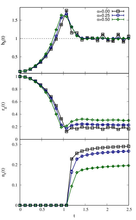
Figure 1: Ensemble-averaged temporal evolutions of the virial ratio of bound mass $b_{b}$ (top panel), the gravitational radius of bound mass $r_{g}$ (middle panel) and the fraction of ejected mass $n_{e}$ (bottom panel) for different indicated $\alpha$ with $b_{0}=0.1$ and $N=64000$. Size of error bars corresponds to the standard deviation of the mean.

We first consider the overall process of violent relaxation for different $\alpha$ and $b_{0}$. Shown in Fig. 1 are ensemble-averaged temporal evolutions of the virial ratios of bound particles $b_{b}$, the gravitational radii of bound particles $r_{g}$ and the fractions of ejected particles $n_{e}$ around the violent relaxation for different $\alpha$ with $b_{0}=0.1$ and $N=64000$. The definition of $r_{g}$ is given by

$$r_{g}=\frac{GM_{b}^{2}}{|U_{b}|}$$ (31)

where $M_{b}$ and $U_{b}$ are the mass and potential energy computed from bound particles. This radius is presented as the unit of distance in the initial value. First, we see that the virializations of the three cases are similar in the way that $b_{b}$ increases from $b_{0}$ by collapse and goes beyond $1$ at $t\sim 1$. It then relaxes down to a virialized state around $1.5\ t_{d}$. Increasing $\alpha$ makes the increment slightly faster and $b_{b}$ reaches slightly lower maximum value. The evolution of $r_{g}$ is consistent with that of $b_{b}$. From its initial value, it decreases and attains a minimum at the time when $b_{b}$ reaches its maximum. It is then brought up to its virialized value. We remark that both the minimum attained and final $r_{g}$ tend to be lower if $\alpha$ decreases, which indicates that the collapse and resulting central core are more compact as $\alpha\rightarrow 0$. This can be explained in the following way. In the fluid limit with $b_{0}=0$, we can prove that all mass is falling to the center in the global free-fall time. In a point system with $b_{0}>0$, the effects from Poissonian noise and velocity dispersion cause the free-fall times of particles to disperse, limiting the compactness from progressing close to a singularity. Furthermore, if $\alpha>0$, the individual free-fall time is longer at larger radial distance, so the time spread is even wider because of $\alpha$ than it would be from Poissonian noise alone. This factor makes the infall more prolonged, resulting in the observed variation of $r_{g}$. The degree of violent collapse also manifests itself in the final values of $n_{e}$ where the particles are ejected more as $\alpha$ decreases from $0.5$ to $0$. The ejection mechanism, described by Joyce et al. (2009), is that the late-arriving particles gain a gravitational slingshot effect from the time-varying central potential formed by the particles that arrive earlier. Thus, the variation of $n_{e}$ also reflects the concentration formed by different $\alpha$. This $\alpha$-dependence of collapse properties has been reported before by Sylos Labini et al. (2015) for $b_{0}=0$ but here we find that the similar behavior is maintained even if $b_{0}>0$.

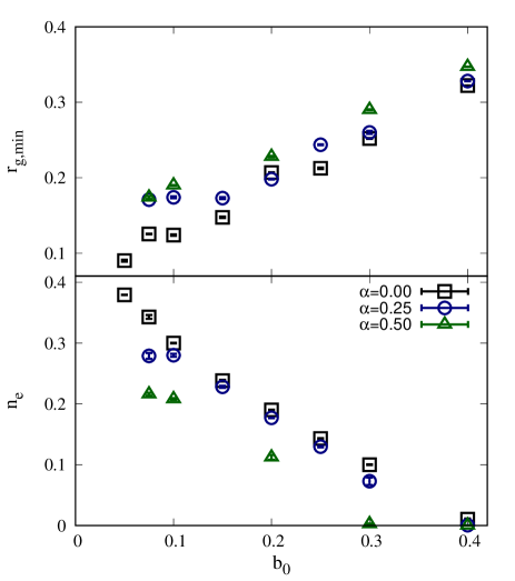
Figure 2: Ensemble-averaged minimum gravitational radius in the collapse $r_{g,min}$ (top panel) and $n_{e}$ at $9.52\ t_{d}$ (bottom panel) as function of $b_{0}$ for $N=64000$. Size of error bars correspond to the standard error of the mean.

Next, we consider the consequence of the violent relaxation from different $b_{0}$. Shown in Fig. 2 are ensemble-averages of the minimum gravitational radius in the collapse ($r_{g,min}$) and $n_{e}$ measured at $9.52\ t_{d}$, plotted as functions of $b_{0}$ for different $\alpha$. All cases include $64,000$ particles. From the overall viewpoint, the behaviors of both parameters indicate that increasing $b_{0}$ can moderate the collapse and the ejection. When $b_{0}\geq 0.2$, the calculated values between $\alpha=0$ and $0.25$ become closer to each other. This implies that the influence of mild $\alpha$ is overcome by the initial pressure. The variation of $n_{e}$ also suggests that there should be no ejection beyond $b_{0}=0.4$. With a closer perspective, we remark that the variations are indeed different at high and low $b_{0}$. When $b_{0}\geq 0.2$, both $r_{g,min}$ and $n_{e}$ vary in the way that we expect from increasing $b_{0}$ since it provides a stronger outward force against the contraction. For $b_{0}<0.2$, we remark that the plots from non-zero $\alpha$ appear to converge to certain values, which are seen more clearly from $n_{e}$ plots. This result can be explained if we consider that in the limit where the influence of $b_{0}$ is not significant, the evolutions of cloud size and concentration mainly depend on the details of density profile. This leads to the ordered infall of each mass shell from a different position. Thus, we generally expect that if $b_{0}\rightarrow 0$, the parameters should converge to non-zero values that depend strongly on $\alpha$, as suggested by Sylos Labini et al. (2015). For $\alpha=0$, there is, on the contrary, no sign of convergence as both parameters change constantly until the lowest shown $b_{0}$. The dissimilarity with previous results may possibly be related to the absence of a density gradient to control the minimum size. As we approach the cold limit, the evolution to maximum contraction is regulated by finite-$N$ fluctuations. However, as suggested by Joyce et al. (2009), it is possible that there also exists the terminal $r_{g,min}$ and $n_{e}$ that now depend on $N$. That value of $b_{0}$ at which they converge might be far below those for $\alpha>0$ since the effect of density fluctuations is much weaker than that of the density gradient. Note that the measurement of $r_{g,min}$ can be done more precisely by increasing time resolution of the snapshot since the attainment to the minimum is momentary in time unlike $n_{e}$, which is seen to be changing less once it is virialized. This issue is peripheral to our study.

4.2 Development of triaxiality for different $\alpha$

In this section, we inspect the development of triaxiality for different initial conditions. Before we start, we recall that the violent relaxation of a collapsing cloud generally yields some amount of mass ejection. We will thus consider the configuration of bound particles only. To quantify it, we define

$$\iota_{\chi}=\frac{\Lambda_{3,\chi}}{\Lambda_{1,\chi}}-1$$ (32)

to be the flattening of $\chi$ percent of most bound mass. In that expression, $\Lambda_{3,\chi}$ and $\Lambda_{1,\chi}$ correspond to the highest and lowest eigenvalues, respectively, of the moment of inertia tensor calculated from $\chi$ percent of most bound particles around their respective center of mass. The flattening of the relaxed structure calculated from $\chi=80$ has been found suitable since it excludes an amount of loosely bound particles that disrupt the calculation of the moment of inertia tensor from the majority of particles (Boily & Athanassoula, 2006; Barnes et al., 2009; Worrakitpoonpon, 2015). However, the tracking of $\iota_{\chi}$ with different $\chi$ values might still be useful as it allows us to observe the development of triaxiality at different levels.

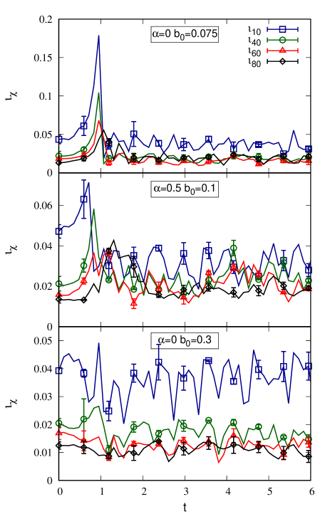
Figure 3: Temporal evolutions of ensemble-averaged different $\iota_{\chi}$ for $\alpha=0$ and $b_{0}=0.075$ (top panel); $\alpha=0.5$ and $b_{0}=0.1$ (middle panel); and $\alpha=0$ and $b_{0}=0.3$ (bottom panel). All of these cases are with $N=64,000$. Size of error bars corresponds to the standard deviation of the mean.

To verify this process, temporal evolutions of ensemble-averages of $\iota_{\chi}$ for three indicated cases with $64,000$ particles are shown in Fig. 3. For $b_{0}\leq 0.1$, $\iota_{\chi}$ is amplified in all levels by anisotropic collapse and reaches the maximum that is a few times larger than its starting value. It then relaxes down to a quasi-stationary state afterwards. Fluctuations are still present after the violent relaxation but the average flattening as evaluated from $\iota_{80}$ is clearly above its initial one. A major difference between the two cases is the time $\iota_{\chi}$ takes to attain maximum during the violent relaxation. For the uniform case, all $\iota_{\chi}$ evolve accordingly and reach their peaks almost at the same time. For $\alpha=0.5$, the peaks shift forward in time as a larger fraction is involved. The different evolutionary patterns of $\iota_{\chi}$ occur because the local free-fall time is uniform and increasing with radius for $\alpha=0$ and $0.5$, respectively. Thus, for the latter case, higher $\chi$ tends to have longer effective collapse time during which the triaxiality is amplified. An analogous plot is illustrated by Boily & Athanassoula (2006) for $b_{0}=0$ and $\alpha=0.5$ that leads to a similar statement as with our $\alpha>0$ case. Here we illustrate clearly the difference between the cases with $\alpha=0$ and $\alpha=0.5$. Otherwise, the plot for $b_{0}=0.3$ demonstrates weak or absent amplification of $\iota_{\chi}$ during the violent relaxation before it relaxes to the virialized state in a similar way. Following our proposed mechanism, the weaker asymmetric field inside, indicated by $\iota_{10}$, results in the suppressed development of $\iota_{\chi}$ for larger mass fractions during this early stage.

According to our proposal, the situations for $b_{0}\leq 0.1$ strictly conform with the original LMS scenario as we observe the effective inside-out amplification of $\iota_{\chi}$. With $b_{0}=0.3$, the core triaxiality cannot be developed much and this consequently limits the amplification of $\iota_{80}$. That the latter evolution progresses in the suppressed way affirms our hypothesis that the LMS deformation process can be inactivated by sufficiently high $b_{0}$, as discussed in Section 2.4.

4.3 Critical particle number in different cases

We will verify in this section the existence and the variation of the critical particle number following our proposition in Section 2. From the computed $\iota_{80}$ in previous section, we choose to evaluate the amplification effectiveness by comparing this parameter at the stationary state with the initial one. Given the ensemble-averaged temporal profile of $\iota_{80}$ in each case, the ratio between virialized $\iota_{80}$, averaged from $7.14$ to $9.52\ t_{d}$ over 20 time-slices, and the initial $\iota_{80}$ (designated by $\overline{\iota_{80}}/\iota_{80,0}$) as function of $N$ for different $\alpha$ and $b_{0}$ is plotted in Fig. 4. Inspecting the result in this way allows us to monitor the intrinsic efficiency more accurately as this ratio is adjusted by the initial $\iota_{80}$ that has been found to decrease as rapidly as $N^{-1/2}$ (Benhaiem & Sylos Labini, 2015). We additionally apply the time average over the period of the stationary state in order to smooth out the temporal fluctuations which is seen to be of order final $\iota_{80}$. Error bars are estimated from the time-averaged standard deviation of the mean in the same time window. The horizontal lines indicate when initial and averaged-final $\iota_{80}$ are equal. From a glance at the plot, we see that a higher $b_{0}$ can suppress more effectively the development of triaxiality, now parametrized by $\overline{\iota_{80}}/\iota_{80,0}$, which is seen in all panels and is in line with the result in Section 4.2.

Figure 4: Ratios between virialized $\iota_{80}$ and initial $\iota_{80}$ (i.e. $\overline{\iota_{80}}/\iota_{80,0}$) as functions of $N$ for different indicated $\alpha$ and $b_{0}$ (see calculation detail in text). Size of error bars corresponds to the standard deviation of the mean.

Considering its variation with $N$, $\overline{\iota_{80}}/\iota_{80,0}$ decreases for $\alpha=0$ and, as evident from this tendency, crosses the separating line at a certain $N$. The cases with no amplification even yield the ratios that are considerably below $1$ although the number of involved particles is reduced by ejection. This implies that when the amplification of triaxiality seeded by density fluctuations is masked by the pressure force, the infall of particles produces more spherical figure than the initial state. With $\alpha=0.25$, we find that $\overline{\iota_{80}}/\iota_{80,0}$ is, on average, higher than that in the previous case. The points vary in different way as they rather fluctuate and drop below the line when $N$ is equal to $32,000$. Unexpectedly, the points for $N=64,000$ and $128,000$ with $b_{0}=0.3$ are located at the upper area despite that the point for $N=32,000$ is below the line. We notice remarkably large error bar for $N=64,000$ that spans both regions. This indicates that the obtained $\overline{\iota_{80}}/\iota_{80,0}$ from two different realizations are very scattered, with one above and one below the line separating two regions. This is the outcome from the finite-$N$ fluctuations where the designation of $b_{0}$ and $N$ alone cannot determine the final triaxiality in each individual realization. Different microscopic arrangements can lead to the final triaxiality that can be either greater or lower than the initial one even with $N$ as high as $64,000$. However, when considering the mean behavior, the first $N$ where the plot crosses or gets close to the separating lines, marking the critical number $N_{c}$, is clearly reduced when $b_{0}$ is higher in both $\alpha$. This is consistent with our hypothesis. When $\alpha=0.5$, the transition is barely seen. This case yields the ratios that are greater than the two previous cases and the development of triaxiality is hardly reduced even though $b_{0}$ is as high as $0.3$: only the case with $N=128,000$ lies below the line whereas the other cases remain far above.

For $\alpha=0$, that $\iota_{80}$ decreases with increasing $b_{0}$, while still remaining above the separating line, can also be explained by an extension of our hypothesis beyond its main purpose for $N_{c}$. According to the analysis in Section 2, the distinction between gravity fluctuation- and pressure-dominated core collapse is made by comparing the values of $r_{J}$ and $\tilde{r}$. While the core collapse is still dominated by $\tilde{r}$, the increase of $b_{0}$ simply gives more resisting force, which is described mathematically by the increase of $r_{J}$ closer to $\tilde{r}$. This leaves less available space for collapse and amplification beneath $\tilde{r}$. Therefore, the amplification degree is reduced, but it is still effective. When $\alpha>0$, $\overline{\iota_{80}}/\iota_{80,0}$ is higher on average and the same variation with $N$ is not noticed because the fluctuating pattern is more prominent. The fact that increasing $\alpha$ tends to yield a more elevated ratio, albeit with a lower collapse factor (see Fig. 2), can be related to the so-called parametric resonance. This effect is summarized in Levin et al. (2014). In principle, a non-zero $\alpha$ triggers non-simultaneous collapse: the inner component falls earlier, forming a dense oscillating core in the process. The resulting oscillating field is then able to resonate with the late infall and the expansion of the outer mass shell. This magnifies the extent of the axis contrast of structure as an additional factor to the LMS instability. With higher $\alpha$, the spread of free-fall times from inside to outside mass shell is widened. So, there should be more resonances possible in the violent relaxation, resulting in higher flattening. In other words, this process of morphological evolution incorporates another $\alpha$-dependent mechanism, in the form of a boost, apart from the essential $N$-dependent LMS instability. This explains why, for $\alpha>0$, the same measured parameter fluctuates above the threshold. It is the remnant of the $\alpha$-dependent virialization. Note that the parametric resonance is also believed to account for the formation of core-halo structure, which is found to be the generic form of the quasi-stationary state achieved from violent relaxation.

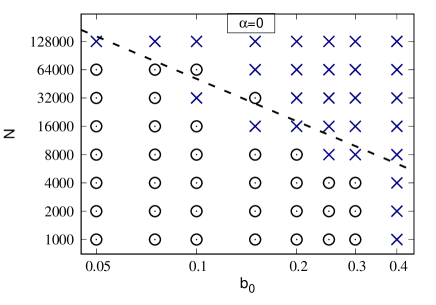
Figure 5: Summary of $\overline{\iota_{80}}/\iota_{80,0}$ in $(b_{0},N)$ space for $\alpha=0$ (top panel) and $0.25$ (bottom panel). The cases for any $b_{0}$ and $N$ with the ratios above (and below) $1.05$ are depicted in circle (and cross). Dash lines are the best-fitting theoretical predictions corresponding to $b_{0}^{-3/2}$ and $b_{0}^{-11/7}$ for $\alpha=0$ and $0.25$, respectively, with $N_{c}$ defined as the lowest $N$ where the ratio turns below the threshold. The fitting excludes the result from $b_{0}=0.4$ in both cases.

The effectiveness of symmetry breaking is summarized in $(b_{0},N)$ diagrams in Fig. 5 where the cases with $\overline{\iota_{80}}/\iota_{80,0}$ above and below $1.05$ are depicted in different ways. By defining $N_{c}$ as the lowest $N$ where the ratio falls below $1.05$, we provide the best-fitting lines of $b_{0}^{-3/2}$ and $b_{0}^{-11/7}$ functions with $N_{c}$ for $\alpha=0$ and $0.25$, respectively. This tests the validity of the hypothesis we gave in Section 2.2 and 2.3. Note that the fitting is performed from the lowest depicted $b_{0}$ to $b_{0}=0.3$. The case with $\alpha=0.5$, for which strong symmetry breaking occurs in almost all cases, is not shown because of insufficient statistics. The plot for $\alpha=0$ exhibits a clear partition by the best-fitting line between upper and lower areas, indicating ineffective and effective amplifications of triaxiality, respectively. We notice a few anomalies, one for each of $b_{0}=0.1$ and $0.15$, where $\overline{\iota_{80}}/\iota_{80,0}$ remains higher than the threshold just above $N_{c}$. Because those cases are situated near the transition line, different statistical fluctuations may lead to very different final triaxiality in each realization. Thus, the ensemble average may have a high dispersion comparing to the cases that are further away from the line. The case of $b_{0}=0.4$ is notable and requires further explanation. The amplification is weak for $N=1,000$, which is far below the prediction line. This implies over-stability. We speculate that when $b_{0}$ is high enough, the inner pressure force that diverges more rapidly than the gravitational force becomes so strong that it expels away the particles in the opposite direction to the infall. It then attenuates the strength of the triaxial field and leads to an ineffective symmetry breaking even if $N$ is as low as $1,000$.

For $\alpha=0.25$, we find that $N_{c}$ at each $b_{0}$ is higher than its $\alpha=0$ counterpart and it still fits well with the predicted separating line until $b_{0}=0.3$. Comparing it with the case of $\alpha=0$, we find a few more anomalies with $b_{0}=0.25$ and $0.3$ where the amplification degree remains high well away from $N_{c}$. The result for $b_{0}=0.4$ gives rise to more complications since, at first, it implies the same over-stability because of weak amplification that is already present with $N=1,000$. It then shows a switch between two regimes with $N$ up to $N=128,000$. Following from the discussion on Fig. 4, these complexities can be attributed to the combined effect when $\alpha>0$. In the situations where structural deformation is triggered, as described by our hypothesis, the violent relaxation of sequential collapse tends to produce higher triaxiality than that which is produced by simultaneous collapse given the same amount of initial $\iota_{80}$. Consequently, the statistical average of the relative $\iota_{80}$, calculated from the populations of strong and weak amplifications, has higher possibility to cross the threshold value. However, this does not contradict our hypothesis since Fig. 5 suggests that, with $\alpha=0.25$, it simply requires higher $N_{c}$ to meet the chosen criterion and those numbers still agree with our prediction. This proves that the proposed estimate of $N_{c}$ can still be valid even if another effect from mild $\alpha$ is incorporated in the evolution. The situation for $\alpha=0.5$ is that the suppression of symmetry breaking is captured only when $N=128,000$ with $b_{0}=0.2$ and $0.3$, also excluding $b_{0}=0.4$ due to the same over-stability referred to above. The fact that it takes place at an extremity in the simulated parameter space leads us to suspect that $N_{c}$ might be higher for this employed range of $b_{0}$. In other words, due to a stronger amplification process for $\alpha=0.5$, we possibly need to further suppress the initial seed by increasing $N$.

As a final remark in this part, we note the presence of a large dispersion even though $N$ is as high as $64,000$ or more (see, e.g., Fig. 4). This is understandable since the particles involved in determining the fate of the final triaxiality are those around $r_{J}$ or $\tilde{r}$, which account for less than $1\%$ of $N$ in a typical range of $b_{0}$. This fact has not been pointed out in many reports in the literatures that explored a simulation space comparable to our high-$N$ range (Theis & Spurzem, 1999; Roy & Perez, 2004; Boily & Athanassoula, 2006; Barnes et al., 2009).

4.4 $N$-dependence of other parameters

In the previous section, we observed the segregation between strong and weak triaxiality that occurs as consequence of different dominant factors in the core collapse. These two regimes can be discriminated efficiently by $\overline{\iota_{80}}/\iota_{80,0}$ and the transition points behave in accordance with the prediction. In this section, we consider some additional widely-employed parameters relating to the collapse and the configuration and examine whether their variations with $N$ exhibit the same transition that we reported. In Fig. 6 we show the ensemble-averaged $\iota_{80}$ and $n_{e}$ at $9.52\ t_{d}$ as functions of $N$ with various $\alpha$ and $b_{0}$. The vertical dashed lines correspond to $N_{c}$ for each case. We consider first the variation of $\iota_{80}$. The plot exhibits clearly the decay with $N$. When we inspect the final $\iota_{80}$, we see that varying $\alpha$ or $b_{0}$ does not strongly affect the results compared to the variation of $N$. Thus, it turns out that the influence of both these parameters is relatively minor below the governance from $N$ in these warm collapse experiments. This is unlike $\overline{\iota_{80}}/\iota_{80,0}$ (see Fig. 4), with which the effect from increasing $\alpha$ and $b_{0}$ can be differentiated. However, the situation is different for $b_{0}=0$ as it is found that the influence of $\alpha$ becomes prominent as reported by Sylos Labini et al. (2015). From their study, the flattening of relaxed structures can be enhanced many times by increasing $\alpha$.

While the $N$-dependence of final $\iota_{80}$ is evident in all plots, its variation does not display the transition in coherence with the vertical line. The reason why the transition cannot be spotted from direct examination on $\iota_{80}$ can be explained as follows. According to the analysis of Lin, Mestel & Shu (1965), the evolutionary track of eccentricity depends strongly on the initial value. It is thus plausible that the output triaxiality also depends on the initial strength of seed. In our set-up, the initial $\iota_{80}$ is governed by the Poissonian noise that can be scaled by $N^{-1/2}$. Therefore, a strong $N$-dependence of final $\iota_{80}$ can be understood since it involves strong $N$-dependent effects from the initial seed to its path of evolution. This explains why the measurement by $\overline{\iota_{80}}/\iota_{80,0}$ is more effective: it weights out the strength of initial fluctuations from evaluation.

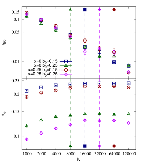
Figure 6: Ensemble-averaged $\iota_{80}$ (top panel) and $n_{e}$ (bottom panel) at $9.52\ t_{d}$ as functions of $N$ for different indicated $\alpha$ and $b_{0}$. Vertical dashed lines with filled points designate $N_{c}$ of the plotted cases in empty points with the same shapes. Size of error bars is estimated by the standard deviation of the mean.

For $n_{e}$, the fraction increases as we increase $N$ before it apparently attains the terminal value at $N\sim 16,000$. Before we consider how consistent it is with $N_{c}$, we should explain this particular pattern of $n_{e}$. First, we recall the analysis of cold collapse by Joyce et al. (2009), which demonstrates that the collapse of a uniform sphere is more condensed as $N$ increases due to smaller density fluctuations. This makes $n_{e}$ increase accordingly because of the stronger kinetic kick by $N$-dependent central condensation. This statement is presumably applicable to our low-$\alpha$ collapse with low $N$ as we observe an analogous variation of $n_{e}$. In this range, the minimal size dictated by density fluctuations is not particularly small so the system can attain this size and re-expand before the bouncing force from the initial pressure can take any action. In other words, the contraction and ejection in this regime are dominantly governed by density fluctuations that leads to the $N$-dependent consequence. When $N$ is high enough, reduced density fluctuations attempt to produce a more condensed collapse before it is eventually prevented by the pressure that limits the collapse to progress further. Thus, in this scenario, the pressure replaces the density fluctuations as the major actor in controlling the mass concentration and the amount of ejection. The fact that the pressure is independent of $N$ and that its fluctuations decay more rapidly with $N$ leads us to deduce that the achieved maximum contraction and resulting ejection are less relying on $N$ than is its low-$N$ counterpart. This explanation also applies to the plots of $n_{e}$ at high $N$.

Although the proposed mechanism to describe the plot of $n_{e}$ implies interplay between gravity and pressure, their transition points do not coincide with the lines of principal transition since these points appear to be displaced more weakly along the $N$-axis. The weak $N$-dependence of the transition points in $n_{e}$ might be because the determination of them does not fully include the fluctuations of the two counter-acting forces, both of which depend strongly on $N$. It is unlike the shape deformation instability that takes the fluctuations of all forces into consideration.

In summary, the demonstrated plots of some standard parameters emphasize once again the usefulness of $\overline{\iota_{80}}/\iota_{80,0}$ in distinguishing between different regimes to test our hypothesis. The transition is completely undetectable in some parameters such as $\iota_{80}$. Although other parameters, e.g. $n_{e}$, appear to exhibit the related transition, these points do not reflect any proximity to our proposed transition.

5 Conclusion

In this work, we numerically investigate the spherical collapse of gravitationally unstable $N$-body systems that cover a considerable range over the power-law index of density $\alpha$, the particle number $N$ and the initial virial ratio $b_{0}$. Our main objective is to resolve whether the collapse exhibits different regime of shape evolution as we vary the system parameters. In parallel, we develop the collapse model used in the pioneering Lin-Mestel-Shu theory (Lin, Mestel & Shu, 1965) by introducing the velocity dispersion to the initial state. For an unstable sphere of particles, we first evaluate the profiles of the gravitational and pressure forces and their fluctuations, involving the Poissonian noise in both spaces. By finding the balances of these forces, two effective radii are obtained. The first one fixes the size of the non-collapsing region similar to the conventional Jeans’ length while the second one indicates at which scale the density fluctuations are dominant over the pressure fluctuations. We regard the latter radius as the size of the triaxial seed from density fluctuations. Depending on which radius is dominant, two different scenarios of shape evolutions are proposed. When the latter radius is dominant, the collapsing core develops further the triaxiality from the Poissonian density fluctuations and leads to the amplification of entire structure accordingly. Otherwise, the amplification of core triaxiality is halted and the collapsing system remains weakly amplified because it lacks a strong triaxial field. The point where the two radii are equal marks the transition, which is parametrized by the critical $N$ above which the amplification turns ineffective. Although our analysis is specific to simple density profile and velocity distribution, we believe that this methodology can also be applicable to other choices of initial states as long as the Poissonian fluctuations are involved. Different distribution functions simply yield different force profiles and values of the relevant parameters.

Considering the numerical results, the tracing of the flattening of different fractions of bound mass justifies the inside-out shape evolution. To inspect more fully our hypothesis, we measure the ratio of the main flattening parameter between the virialized and initial states (or $\overline{\iota_{80}}/\iota_{80,0}$) as the main tool. This measurement proves effective as it weights out strong $N$-dependence from initial numerical value fixed by the initial density fluctuations. In doing this, many crucial results are unveiled. First, as supposed to be the utility of it, the segregation between effective and ineffective symmetry breaking by the critical particle number is definitely identified. The variation of critical $N$ as function of $b_{0}$ agrees with our prediction in the range of lowest performed $b_{0}$ to $0.3$ provided that $\alpha\leq 0.25$. As $b_{0}$ reaches $0.4$, the flattening process appears to be inactivated in almost all cases. We speculate that this is because of excessive pressure force that expels away the particles in the core. About the influence of $\alpha$, the increase of it from $0$ to $0.25$ not only produces higher flattening, as suggested by past literatures, but it also raises the critical $N$ for the same $b_{0}$. This is possibly due to another $\alpha$-dependent amplifying process from non-simultaneous infall in addition to that fuelled by the LMS instability. The fact that our prediction is still quantitatively valid despite the involvement from mild $\alpha$ assures that the hypothesis of the interplay between two competing forces at two orders in the core is applicable. The situation for $\alpha=0.5$ is more complicated but it is however comprehensible by the same speculation. In this case, the involvement from $\alpha$ plays more significant role to further elevate the ratio. Even faint triaxiality at start could end up highly flattened by the combined procedure. As consequence, almost all cases remain far from initial flattening and only few cases with highest $N$ and high $b_{0}$ are subdued. This suggests that the critical $N$ is higher.

From the conclusion, it appears that the gravitational collapse is more complicated than the proposed description that is on the basis of the self-consistent LMS framework alone. Other known astrophysical mechanisms such as the parametric resonance or the radial orbit instability might also come into play even if the initial density profile slightly deviates from homogeneity. The combined process leads to another degree of amplification. This makes us uncertain about the validity of our hypothesis beyond mildly inhomogeneous density profile since the non-LMS driving process is more prominent.

6 Discussion

In this section, we discuss the related studies in the past. From analytical point of view, we note an analogous work of Boily et al. (2002) where they also analyzed the cold collapse to determine the critical particle number. Their number indicates other transition where, exceeding this number, the Poissonian fluctuations cease to have influence on a mildly ellipsoidal collapse. Consequently, the evolution strictly follows the LMS pattern. This work has the same conception such that, above the critical particle number, the influence of Poissonian fluctuations on the violent relaxation is limited. However, without pre-adjusted ellipticity, a cold spherical collapse is always unstable according to our hypothesis since there is no pressure. Considering then the numerical results, our work demonstrates the role of $N$ in quite the same way as shown by Benhaiem et al. (2018). This group carries out the spherical collapse experiments with $\alpha=1$ and, as first expectation, obtains far greater $\iota_{80}$ compared to our $\alpha=0.5$ simulations. Similarly, they exemplify the suppression of the onset of the radial orbit instability following the collapse by increasing $N$. While the driving mechanism is different, the fact that reducing the amplitude of initial fluctuations by increasing $N$ is able to turn off the key process that breaks strongly the symmetry relates closely to our scope. However, more quantitative evaluation of the transition point has been omitted there. About the attempt to retrieve the critical values, Min & Choi (1989) have investigated the collapse of a sphere with uniform density and proposed an upper limit with $b_{0}=0.3$, below which the symmetry breaking is efficient. Next, Boily & Athanassoula (2006) have performed a similar investigation for the cases with non-uniform density profiles and reported the limiting $b_{0}=0.4$. This latter value coincides with a part of our summary but this suppression is caused by an excessive kinetic energy in the core which is out of the main scope.

Before we continue the discussion, we should make the relation between the parameters clear. Although their employed parameter to pinpoint the transition is different from ours, the diagrams in Fig. 5 suggest that these two parameters are interchangeable: we can draw either the critical $N$ at the given $b_{0}$ or the critical $b_{0}$ at the given $N$. According to our finding, it appears that some crucial points are missing in those works. First, the practice to examine the final flattening parameter without considering the initial value and then to specify an arbitrarily small value for a transition might not be sufficient to give an accountable critical point. Note that there are also the temporal and ensemble fluctuations in the relaxed states. This causes, on the one hand, the improper identification of the critical value or, on the other hand, the unawareness of the transition while varying $b_{0}$ (van Albada, 1982; McGlynn, 1984; Roy & Perez, 2004). The next point is that a certain critical $b_{0}$ is actually not applicable to all systems since we find that it changes significantly from one initial state to another. For example, given the same initial density profile, the critical $b_{0}$ significantly shifts as we simply change $N$. We would additionally mention that in some cases, e.g. the power-law density profile with high exponent, the critical number might be beyond the executable $N$, if evaluated in our way. Our results with $\alpha=0.5$ already give an example of that claim.

Data availability

The data used in this article can be shared on reasonable request to the corresponding author.

References

- Aarseth & Binney (1978) Aarseth S. J., Binney J., 1978, Mon. Not. R. Astr. Soc., 185, 227
- Aarseth et al. (1988) Aarseth S. J., Lin D. N. C., Papaloizou J. C. B., 1988, Astrophys. J., 324, 288
- Aguilar & Merritt (1990) Aguilar L. A., Merritt D., 1990, Astrophys. J., 354, 33
- Barnes et al. (2009) Barnes E. I., Lanzel P. A., Williams L. L. R., 2009, Astrophys. J., 704, 372
- Benhaiem & Sylos Labini (2015) Benhaiem D., Sylos Labini F., 2015, Mon. Not. R. Astr. Soc., 448, 2634
- Benhaiem et al. (2018) Benhaiem D., Joyce M., Sylos Labini F., Worrakitpoonpon T., 2018, Mon. Not. R. Astr. Soc., 473, 2348
- Boily & Athanassoula (2006) Boily C. M., Athanassoula E., 2006, Mon. Not. R. Astr. Soc., 369, 608
- Boily et al. (2002) Boily C. M., Athanassoula E., Kroupa P., 2002, Mon. Not. R. Astr. Soc., 332, 971
- Cannizzo & Hollister (1992) Cannizzo J. K., Hollister T. C., 1992, Astrophys. J., 400, 58
- Joyce et al. (2009) Joyce M., Marcos B., Sylos Labini F., 2009, Mon. Not. R. Astr. Soc., 397, 775
- Levin et al. (2014) Levin Y., Pakter R., Rizzato F. B., Teles T. N., Benetti F. P. C., 2014, Phys. Rep., 535, 1
- Lin et al. (1965) Lin C. C., Mestel L., Shu F. H., 1965, Astrophys. J., 142, 1431
- Lynden-Bell (1967) Lynden-Bell D., 1967, Mon. Not. R. Astr. Soc., 136, 101
- McGlynn (1984) McGlynn T. A., 1984, Astrophys. J., 281, 13
- Min & Choi (1989) Min K. W., Choi C. S., 1989, Mon. Not. R. Astr. Soc., 238, 253
- Roy & Perez (2004) Roy F., Perez J., 2004, Mon. Not. R. Astr. Soc., 348, 62
- Springel (2005) Springel V., 2005, Mon. Not. R. Astr. Soc., 364, 1105
- Springel et al. (2001) Springel V., Yoshida N., White S. D. M., 2001, New Astron., 6, 79
- Sylos Labini (2012) Sylos Labini F., 2012, Mon. Not. R. Astr. Soc., 423, 1610
- Sylos Labini (2013) Sylos Labini F., 2013, Mon. Not. R. Astr. Soc., 429, 679
- Sylos Labini et al. (2015) Sylos Labini F., Benhaiem D., Joyce M., 2015, Mon. Not. R. Astr. Soc., 449, 4458
- Theis & Spurzem (1999) Theis C., Spurzem R., 1999, Astron. Astrophys., 341, 361
- Worrakitpoonpon (2015) Worrakitpoonpon T., 2015, Mon. Not. R. Astr. Soc., 446, 1335
- de Vaucouleurs (1953) de Vaucouleurs G., 1953, Mon. Not. R. Astr. Soc., 113, 134
- van Albada (1982) van Albada T. S., 1982, Mon. Not. R. Astr. Soc., 201, 939