Conditions for indexability of restless bandits and an $\mathcal{O}(K^{3})$ algorithm to compute Whittle index

Abstract

Restless bandits are a class of sequential resource allocation problems concerned with allocating one or more resources among several alternative processes where the evolution of the process depends on the resource allocated to them. Such models capture the fundamental trade-offs between exploration and exploitation. In 1988, Whittle developed an index heuristic for restless bandit problems which has emerged as a popular solution approach due to its simplicity and strong empirical performance. The Whittle index heuristic is applicable if the model satisfies a technical condition known as indexability. In this paper, we present two general sufficient conditions for indexability and identify simpler to verify refinements of these conditions. We then revisit a previously proposed algorithm called adaptive greedy algorithm which is known to compute the Whittle index for a subclass of restless bandits. We show that a generalization of the adaptive greedy algorithm computes the Whittle index for all indexable restless bandits. We present an efficient implementation of this algorithm which can compute the Whittle index of a restless bandit with $K$ states in $\mathcal{O}(K^{3})$ computations. Finally, we present a detailed numerical study which affirms the strong performance of the Whittle index heuristic.

Nima Akbarzadeh and Aditya Mahajan

[McGill University]Nima Akbarzadeh[McGill University]Aditya MahajanDepartment of Electrical and Computer Engineering, McGill University, 3480 Rue University, Montréal, QC H3A 0E9.

90C4090C39;49M20;91B32

1 Introduction

Restless bandits are a class of sequential resource allocation problems concerned with allocating one or more resources among several alternative processes where the evolution of the process depends on the resource allocated to them. Such models arise in various applications such as machine maintenance [18], congestion control [6], healthcare [10], finance [15], channel scheduling [21], smart grid [1], and others.

Restless bandits are a generalization of classical multi-armed bandits [13], where the processes remain frozen when resources are not allocated to them. Gittins [14] showed that when a single resource is to be allocated among multiple processes, the optimal policy has a simple structure: compute an index for each process and allocate the resource to the process with the largest (or the lowest) index. In contrast, the general restless bandit problem is pspace-hard [27]. Whittle [32] showed that index-based policies are optimal for the Lagrangian relaxation of the restless bandit problem and argued that the corresponding index, now called Whittle index, is a reasonable heuristic for restless bandit problems. Subsequently, it has been shown that the Whittle index heuristic is optimal under some conditions [31, 22] and performs well in practice [4, 19, 16].

The Whittle index heuristic is applicable if a technical condition known as indexability is satisfied. Sufficient conditions for indexability have been investigated under specific modeling assumptions: two state restless bandits [21, 6]; monotone bandits [15, 4, 6]; models with right-skip free transitions [18, 19]; models with monotone or convex cost/reward [19, 4, 6, 5, 33, 7]; models satisfying partial conservation laws [23, 25]; and models arising in specific applications [16, 18, 19, 5, 7].

Nino-Mora [26, 25] proposed a generalization of Whittle index called marginal productivity index (MPI) for resource allocation problems where processes can be allocated fractional resources. In [25], he also proposed an algorithm called the adaptive greedy algorithm, to compute the MPI when the model satisfies a technical condition called partial conservation laws (PCL). For restless bandits which satisfy the PCL condition, the Whittle index can be computed using the adaptive greedy algorithm. However, for general restless bandits, there are no known efficient algorithms to exactly compute the Whittle index. It is possible to approximately compute the Whittle index by conducting a binary search over penalty for active action (or a subsidy for passive action) [29, 2] but such a binary search is computationally expensive because each step of the binary search requires solving a dynamic program.

In this paper, we revisit the restless bandit problem and present three contributions. Our first contribution is to provide general sufficient conditions for indexability which are based on an alternative characterization of the passive set. We also present easy to verify refinements of these sufficient conditions.

Our second contribution is to use a novel geometric interpretation of Whittle index to show that a refinement of the adaptive greedy algorithm proposed by Nino-Mora [25] computes the Whittle index for all indexable restless bandits. We provide a computationally efficient implementation, which computes the Whittle indices of a restless bandit with $K$ states in $\mathcal{O}(K^{3})$ computations.

Our third contributions is to present three special cases: (i) Restless bandits with optimal threshold-based policy which were previously studied in [4, 17, 6, 15, 30, 3], (ii) Stochastic monotone bandits which may be considered as a generalization of monotone bandits [15, 4, 6], and (iii) Restless bandits with controlled restarts similar to [3, 30], which is a generalizations of the restart models [18, 19]. We show that these models are always indexable and the Whittle index can be computed in closed form.

Finally, we present a detailed numerical study comparing the performance of the Whittle index policy with that of the optimal and myopic policies. Our study shows that in general, the performance of Whittle index policy is comparable to the optimal policy and considerably better than the myopic policy.

Notation

Uppercase letters ($X$, $Y$, etc.) denote random variables, lowercase letters ($x$, $y$, etc.) denote their realization, and script letters ($\mathcal{X}$, ${\cal Y}$, etc.) denote their state spaces. Subscripts denote time: so, $X_{t}$ denotes a system variable at time $t$ and $X_{1:t}$ is a short-hand for the system variables $(X_{1},\dots,X_{t})$. $\mathds{P}(\cdot)$ denotes the probability of an event, $\mathds{E}[\cdot]$ denotes the expectation of a random variable. $\mathbb{Z}$ and $\mathbb{R}$ denote the sets of integers and real numbers. Given a matrix $P$, $P_{ij}$ denotes its $(i,j)$-th element.

2 Restless bandits: problem formulation and solution concept

2.1 Restless Bandit Process

A discrete-time restless bandit process (RB) is a controlled Markov process $(\mathcal{X},\{0,1\},\allowbreak\{P(a)\}_{a\in\{0,1\}},c,x_{0})$ where $\mathcal{X}$ denotes the state space which is a finite or countable set; $\{0,1\}$ denotes the action space where the action $0$ is called the passive action and the action $1$ is the active action; $P(a)$, $a\in\{0,1\}$, denotes the transition matrix when action $a$ is chosen; $c:\mathcal{X}\times\{0,1\}\to\mathbb{R}$ denotes the cost function; and $x_{0}$ denotes the initial state. We use $X_{t}$ and $A_{t}$ to denote the action of the process at time $t$. The process evolves in a controlled Markov manner, i.e., for any realization $x_{0:t+1}$ of $X_{0:t+1}$ and $a_{0:t+1}$ of $A_{0:t+1}$, we have $\mathds{P}({X}_{t+1}={x}_{t+1}|{X}_{0:t}={x}_{0:t},{A}_{0:t}={a}_{0:t})=\mathds{P}(X_{t+1}=x_{t+1}|X_{t}=x_{t},A_{t}=a_{t})$, which we denote by $P_{x_{t}x_{t+1}}(a_{t})$.

2.2 Restless Multi-armed Bandit Problem

A restless multi-armed bandit is a collection of $n$ independent RBs $(\mathcal{X}^{i},\{0,1\},\allowbreak\{P^{i}(a)\}_{a\in\{0,1\}},c^{i},x^{i}_{0})$, $i\in{\cal N}\coloneqq\{1,\ldots,n\}$. A decision maker observes the state of all RBs, may choose to activate only $m<n$ of them, and incurs a cost equal to the sum of the cost incurred by each RB.

Let $\boldsymbol{\mathcal{X}}\coloneqq\prod_{i\in\cal N}\mathcal{X}^{i}$ and ${\mathbfcal A}(m)\coloneqq\bigl{\{}{\boldsymbol{a}}=(a^{1},\ldots,a^{n})\in{\cal A}^{n}:\sum_{i\in{\cal N}}a^{i}=m\bigr{\}}$ denote the joint state space and the feasible action space, respectively. Let ${\boldsymbol{X}}_{t}\coloneqq(X^{1}_{t},\dots X^{n}_{t})$ and ${\boldsymbol{A}}_{t}=(A^{1}_{t},\dots,A^{n}_{t})$ denote the joint state and actions at time $t$. As the RBs evolve independently, for any realization ${\boldsymbol{x}}_{0:t}$ of ${\boldsymbol{X}}_{0:t}$ and ${\boldsymbol{a}}_{0:t}$ of ${\boldsymbol{A}}_{0:t}$, we have $\mathds{P}\left({\boldsymbol{X}}_{t+1}={\boldsymbol{x}}_{t+1}|{\boldsymbol{X}}_{0:t}={\boldsymbol{x}}_{0:t},{\boldsymbol{A}}_{0:t}={\boldsymbol{a}}_{0:t}\right)=\prod_{i=1}^{n}\mathds{P}\left(X^{i}_{t+1}=x^{i}_{t+1}|X^{i}_{t}=x^{i}_{t},A^{i}_{t}=a^{i}_{t}\right).$ When the system is in state ${\boldsymbol{x}}_{t}=(x^{1}_{t},\ldots,x^{n}_{t})$ and the decision-maker chooses action ${\boldsymbol{a}}_{t}=(a^{1}_{t},\ldots,a^{n}_{t})$, the system incurs a cost $\bar{c}({\boldsymbol{x}}_{t},{\boldsymbol{a}}_{t})\coloneqq\sum_{i\in{\cal N}}c^{i}(x^{i}_{t},a^{i}_{t})$. The decision-maker chooses his actions using a time-homogeneous Markov policy ${\boldsymbol{g}}:{\mathbfcal X}\to{\mathbfcal A}(m)$, i.e., chooses ${\boldsymbol{A}}_{t}={\boldsymbol{g}}({\boldsymbol{X}}_{t})$. The performance of any Markov policy ${\boldsymbol{g}}$ is given by

$$J^{({\boldsymbol{g}})}({\boldsymbol{x}}_{0})\coloneqq(1-\beta)\mathds{E}\biggl{[}\sum_{t=0}^{\infty}\beta^{t}\bar{c}({\boldsymbol{X}}_{t},{\boldsymbol{g}}({\boldsymbol{X}}_{t}))\bigg{|}{\boldsymbol{X}}_{0}={\boldsymbol{x}}_{0}\biggr{]},$$

where $\beta\in(0,1)$ is the discount factor and ${\boldsymbol{x}}_{0}$ is the initial state of the system.

We are interested in the following optimization problem.

Problem 2.1

Given the discount factor $\beta\in(0,1)$, the total number $n$ of arms, the number $m$ of active arms, RBs $(\mathcal{X}^{i},\{0,1\},\{P^{i}(a)\}_{a\in\{0,1\}},c^{i},x^{i}_{0})$, $i\in{\cal N}$, and initial state ${\boldsymbol{x}}_{0}\in{\mathbfcal X}$, choose a Markov policy ${\boldsymbol{g}}\colon{\mathbfcal X}\to{\mathbfcal A}(m)$ that minimizes $J^{({\boldsymbol{g}})}({\boldsymbol{x}}_{0})$.

Problem 2.1 is a multi-stage stochastic control problem and one can obtain an optimal solution using dynamic programming. However, the dynamic programming solution is intractable for large $n$ since the cardinality of the state space is $\prod_{i\in{\cal N}}|\mathcal{X}^{i}|$, which grows exponentially with $n$. In the next section, we describe a heuristic known as Whittle index to efficiently obtain a suboptimal solution of the problem.

2.3 Indexability and the Whittle index

Consider a RB $(\mathcal{X},\{0,1\},\{P(a)\}_{a\in\{0,1\}},c,x_{0})$. For any $\lambda\in\mathbb{R}$, we consider a Markov decision process $\{\mathcal{X},\{0,1\},\{P(a)\}_{a\in\{0,1\}},c_{\lambda},x_{0}\}$, where

$$c_{\lambda}(x,a)\coloneqq c(x,a)+\lambda a,\quad\forall x\in\mathcal{X},\forall a\in\{0,1\}.$$ (1)

The parameter $\lambda$ may be viewed as a penalty for taking active action. The performance of any time-homogeneous policy $g:\mathcal{X}\to\{0,1\}$ is

$$J^{(g)}_{\lambda}(x_{0}):=(1-\beta)\mathds{E}\biggl{[}\sum_{t=0}^{\infty}\beta^{t}c_{\lambda}(X_{t},g(X_{t}))\bigg{|}X_{0}=x_{0}\biggr{]}.$$ (2)

Consider the following optimization problem.

Problem 2.2

Given the RB $(\mathcal{X},\{0,1\},\{P(a)\}_{a\in\{0,1\}},c_{\lambda},x_{0})$ and the discount factor $\beta\in(0,1)$, choose a Markov policy $g:\mathcal{X}\to\{0,1\}$ to minimize $J_{\lambda}^{(g)}(x_{0})$.

Problem 2.2 is also a Markov decision process and one can obtain an optimal solution using dynamic programming. Let $V_{\lambda}:\mathcal{X}\to\mathbb{R}$ be the unique fixed point of the following:

$$V_{\lambda}(x)=\min\bigl{\{}H_{\lambda}(x,0),H_{\lambda}(x,1)\bigr{\}},\quad\forall x\in\mathcal{X},$$ (3)

where

$$H_{\lambda}(x,a)=(1-\beta)c_{\lambda}(x,a)+\beta\sum_{y\in\mathcal{X}}P_{xy}(a)V_{\lambda}(y),\quad a\in\{0,1\}.$$ (4)

Let $g_{\lambda}(x)$ denote the minimizer of the right hand side of $\eqref{eqn:bllmn_vf}$ where we set $g_{\lambda}(x)=1$ if $H_{\lambda}(x,0)=H_{\lambda}(x,1)$. Then, from Markov decision theory [28], we know that the time-homogeneous policy $g_{\lambda}$ is optimal for Problem 2.2.

Define the passive set ${\Pi}_{\lambda}$ to be the set of states where passive action is optimal, i.e.,

$${\Pi}_{\lambda}\coloneqq\left\{x\in\mathcal{X}:g_{\lambda}(x)=0\right\}.$$ (5)

Definition 2.3 (Indexability)

An RB is indexable if ${\Pi}_{\lambda}$ is increasing in $\lambda$, i.e., for any $\lambda^{\prime},\lambda^{\prime\prime}\in\mathbb{R}$, $\lambda^{\prime}\leq\lambda^{\prime\prime}$ implies that ${\Pi}_{\lambda^{\prime}}\subseteq{\Pi}_{\lambda^{\prime\prime}}$.

Definition 2.4 (Whittle index)

The Whittle index of state $x$ of an indexable RB is the smallest value of $\lambda$ for which $x$ is part of the passive set ${\Pi}_{\lambda}$, i.e., $w(x)=\inf\left\{\lambda\in\mathbb{R}:x\in{\Pi}_{\lambda}\right\}.$

Alternatively, the Whittle index $w(x)$ is a value of the penalty $\lambda$ for which the optimal policy is indifferent between taking active and passive action when the RB is in state $x$.

2.4 Whittle Index Heuristic

A restless multi-armed bandit problem is said to be indexable if all RBs are indexable. For indexable problems, the Whittle index heuristic is as follows: Compute the Whittle indices of all arms offline. Then, at each time, obtain the Whittle indices of the current state of all arms and play arms with the $m$ largest Whittle indices.

As mentioned earlier, Whittle index policy is a popular approach for restless bandits because: (i) its complexity is linear in the number of alternatives and (ii) it often performs close to optimal in practice [4, 19, 16]. However, there are only a few general conditions to check indexability for general models.

2.5 Alternative characterizations of passive set

We now present alternative characterizations of passive set, which is important for the sufficient conditions of indexability that we provide later.

Let $\Sigma$ denote the family of all stopping times with respect to the natural filtration of $\{X_{t}\}_{t\geq 0}$. For any state $x\in\mathcal{X}$, penalty $\lambda\in\mathbb{R}$, and stopping time $\tau\in\Sigma$, define

$$M(x,\tau) \coloneqq\mathds{E}\bigl{[}\beta^{\tau}|X_{0}=x,\{A_{t}=0\}_{t=0}^{\tau-1}\bigr{]},$$

$$L(x,\tau) \coloneqq\mathds{E}\Big{[}\sum_{t=0}^{\tau-1}\beta^{t}c(X_{t},0)+\beta^{\tau}c(X_{\tau},1)\Bigm{|}X_{0}=x,\{A_{t}=0\}_{t=0}^{\tau-1}\Big{]},$$

$$W_{\lambda}(x) \coloneqq(1-\beta)\lambda+\beta\sum_{y\in\mathcal{X}}P_{xy}(1)V_{\lambda}(x).$$ (6)

Let $h_{\tau,\lambda}$ denote the (history dependent) policy that takes passive action up to time $\tau-1$, active action at time $\tau$, and then follows the optimal policy $g_{\lambda}$ (for Problem 2.2). We now present different characterizations of the passive set.

Proposition 2.5

The following characterizations of the passive set are equivalent.

• $\Pi^{(a)}_{\lambda}=\{x\in\mathcal{X}:g_{\lambda}(x)=0\}$

• $\Pi^{(b)}_{\lambda}=\{x\in\mathcal{X}:H_{\lambda}(x,0)<H_{\lambda}(x,1)\}$

• $\Pi^{(c)}_{\lambda}=\{x\in\mathcal{X}:\exists\sigma\in\Sigma,\sigma\neq 0,\text{such that }J^{(h_{\sigma,\lambda})}_{\lambda}(x)<J^{(h_{0})}_{\lambda}(x)\}$

• $\Pi^{(d)}_{\lambda}=\{x\in\mathcal{X}:\exists\sigma\in\Sigma,\sigma\neq 0,\text{such that }(1-\beta)\left(L(x,\sigma)-c(x,1)\right)<W_{\lambda}(x)-\mathds{E}[\beta^{\sigma}W_{\lambda}(X_{\sigma})|X_{0}=x]\}$

See Appendix A for proof.

3 Sufficient Conditions for Indexability

In this section, we identify sufficient conditions for a RB to be indexable.

3.1 Preliminary results

Consider a RB $(\mathcal{X},\{0,1\},\{P(a)\}_{a\in\{0,1\}},c,x_{0})$. For any Markov policy $g\colon\mathcal{X}\to\{0,1\}$ and $\lambda\in\mathbb{R}$, we can write

$$J^{(g)}_{\lambda}(x)=D^{(g)}(x)+\lambda N^{(g)}(x),$$ (7)

where

$$D^{(g)}(x) \coloneqq(1-\beta)\mathds{E}\bigg{[}\sum_{t=0}^{\infty}\beta^{t}c(X_{t},g(X_{t}))\bigg{|}X_{0}=x\bigg{]}$$

and

$$N^{(g)}(x) \coloneqq(1-\beta)\mathds{E}\bigg{[}\sum_{t=0}^{\infty}\beta^{t}g(X_{t})\bigg{|}X_{0}=x\bigg{]}$$

are the expected discounted total cost and the expected number of activations under policy $g$ starting at initial state $x$. $D^{(g)}(\cdot)$ and $N^{(g)}(\cdot)$ can be computed using policy evaluation formulas. In particular, define $P^{(g)}\colon\mathcal{X}\times\mathcal{X}\to\mathbb{R}$ and $c^{(g)}\colon\mathcal{X}\to\mathbb{R}$ as follows: $P^{(g)}_{xy}=P_{xy}(g(x))\text{ and }c^{(g)}_{\lambda}(x)=c_{\lambda}(x,g(x))=c^{(g)}(x,g(x))+\lambda g(x)$ for any $x\in\mathcal{X}$. We also view $g$ as an element in $\{0,1\}^{|\mathcal{X}|}$. Then, using the policy evaluation formula for infinite horizon MDPs [28], we obtain

$$D^{(g)}(x)=(1-\beta)\bigl{[}(I-\beta P^{(g)})^{-1}c^{(g)}\bigr{]}(x)\text{ and }N^{(g)}(x)=(1-\beta)\bigl{[}(I-\beta P^{(g)})^{-1}g\bigr{]}(x).$$ (8)

Figure 1: An illustration of the plot of $J^{(\cdot)}_{\lambda}(x)$ versus $\lambda$ for $g\in{\cal G}:=\{h_{1},h_{2},h_{3}\}$. Let $\lambda^{ij}_{c}$ denote the $\lambda$-value of the intersection of $J^{(h_{i})}_{\lambda}(x)$ and $J^{(h_{j})}_{\lambda}(x)$. Note that in this plot, for all $\lambda\in(-\infty,\lambda^{12}_{c}]$ the policy $h_{1}$ is optimal; for all $\lambda\in[\lambda^{12}_{c},\lambda^{23}_{c}]$ the policy $h_{2}$ is optimal; and for all $\lambda\in[\lambda^{23}_{c},\infty)$ the policy $h_{3}$ is optimal. The lower concave envelope of $J^{(h_{i})}_{\lambda}(x)$ (shown as a thick line) is the value function $V_{\lambda}(x)$, which is piecewise linear, concave, increasing and continuous.

We now provide a geometric interpretation of the value function $V_{\lambda}(x)$ as a function of $\lambda$. For any $g\in{\cal G}$, the plot of $J^{(g)}_{\lambda}(x)=D^{(g)}(x)+\lambda N^{(g)}(x)$ as a function of $\lambda$ is a straight line with $y$-intercept $D^{(g)}(x)$ and slope $N^{(g)}(x)$. By definition, $V_{\lambda}(x)=\inf_{g\in{\cal G}}J^{(g)}_{\lambda}(x).$ Thus, $V_{\lambda}(x)$ is the lower concave envelope of the family of straight lines $\{J^{(g)}_{\lambda}(x)\}_{g\in{\cal G}}$. See Fig. 1 for an illustration. Thus, we have the following:

Lemma 3.1

For any $x\in\mathcal{X}$, $V_{\lambda}(x)$ is continuous, increasing, piece-wise linear and concave in $\lambda$. Furthermore, when ${\cal X}$ is finite, $V_{\lambda}(x)$ is piecewise linear.

Proof 3.2

For any Markov policy $g$, $N^{(g)}(x)$ is non-negative. Therefore, $J^{(g)}_{\lambda}(x)=D^{(g)}(x)+\lambda N^{(g)}(x)$ is increasing and continuous in $\lambda$. Since $V_{\lambda}(x)$ is an infimization of a family of linear functions, it is concave (see Fig. 1). In addition, as monotonicity and continuity are preserved under infimization, the value function is also increasing and continuous in $\lambda$. Finally, when ${\cal X}$ is finite, there are only finite number of pieces. Thus, $V_{\lambda}(x)$ is the minimum of a finitely many linear functions and hence, piece-wise linear.

Lemma 3.3

For any $\lambda^{\prime},\lambda^{\prime\prime}\in\mathbb{R}$,

$$(\lambda^{\prime\prime}-\lambda^{\prime})N^{(g_{\lambda^{\prime\prime}})}(x)\leq V_{\lambda^{\prime\prime}}(x)-V_{\lambda^{\prime}}(x)\leq(\lambda^{\prime\prime}-\lambda^{\prime})N^{(g_{\lambda^{\prime}})}(x),\quad\forall x\in\mathcal{X}.$$

Consequently, $N^{(g_{\lambda})}(x)$ is non-increasing in $\lambda$.

Proof 3.4

Recall that $V_{\lambda}(x)=J^{(g_{\lambda})}_{\lambda}(x)\leq J^{(g_{\lambda^{\prime}})}_{\lambda}(x)$ for any $\lambda^{\prime}\neq\lambda$. Thus,

$$V_{\lambda^{\prime\prime}}(x)-V_{\lambda^{\prime}}(x) =J^{(g_{\lambda^{\prime\prime}})}_{\lambda^{\prime\prime}}(x)-J^{(g_{\lambda^{\prime}})}_{\lambda^{\prime}}(x)\leq J^{(g_{\lambda^{\prime}})}_{\lambda^{\prime\prime}}(x)-J^{(g_{\lambda^{\prime}})}_{\lambda^{\prime}}(x)$$

$$\stackrel{{\scriptstyle(a)}}{{=}}(\lambda^{\prime\prime}-\lambda^{\prime})N^{(g_{\lambda^{\prime}})}(x),$$ (9)

where $(a)$ follows from (7). Similarly, we have

$$V_{\lambda^{\prime\prime}}(x)-V_{\lambda^{\prime}}(x) =J^{(g_{\lambda^{\prime\prime}})}_{\lambda^{\prime\prime}}(x)-J^{(g_{\lambda^{\prime}})}_{\lambda^{\prime}}(x)\geq J^{(g_{\lambda^{\prime\prime}})}_{\lambda^{\prime\prime}}(x)-J^{(g_{\lambda^{\prime\prime}})}_{\lambda^{\prime}}(x)$$

$$\stackrel{{\scriptstyle(a)}}{{=}}(\lambda^{\prime\prime}-\lambda^{\prime})N^{(g_{\lambda^{\prime\prime}})}(x),$$ (10)

where $(a)$ follows from (7). The result follows from combining the above inequalities.

3.2 Sufficient conditions for indexability

Theorem 3.5

Define $\mathcal{H}=\{(g,h):g,h\colon\mathcal{X}\to\{0,1\}\text{ such that for all }x\in\mathcal{X},N^{(g)}(x)\geq N^{(h)}(x)\}$. Each of the following is a sufficient condition for Whittle indexability:

• For any $g,h\in\mathcal{H}$, we have that for every $x,z\in\mathcal{X}$,

  $$\sum_{y\in\mathcal{X}}\Bigl{\{}\bigl{[}\beta P_{zy}(1)-P_{xy}(1)\bigr{]}^{+}N^{(g)}(y)-\bigl{[}P_{xy}(1)-\beta P_{zy}(1)\bigr{]}^{+}N^{(h)}(y)\Bigr{\}}\leq\frac{(1-\beta)^{2}}{\beta}.$$ (11)

• For any $g,h\in\mathcal{H}$, we have that for every $x\in\mathcal{X}$,

  $$\sum_{y\in\mathcal{X}}\Bigl{\{}\bigl{[}P_{xy}(0)-P_{xy}(1)\bigr{]}^{+}N^{(g)}(y)-\bigl{[}P_{xy}(1)-P_{xy}(0)\bigr{]}^{+}N^{(h)}(y)\Bigr{\}}\leq\frac{1-\beta}{\beta}.$$ (12)

See Appendix B for the proof. The sufficient conditions of Theorem 3.5 can be difficult to verify. Simpler sufficient conditions are stated below.

Proposition 3.6

Each of the following is a sufficient condition for (11).

1. $\max_{x,z\in\mathcal{X}}\sum_{y\in\mathcal{X}}\bigl{[}\beta P_{zy}(1)-P_{xy}(1)\bigr{]}^{+}\leq(1-\beta)^{2}/\beta$.

2. $P_{xy}(1)=P_{zy}(1)$, for any $x,y,z\in\mathcal{X}$.

In addition, each of the following is a sufficient condition for (12).

1. $\max_{x\in\mathcal{X}}\sum_{y\in\mathcal{X}}\left[P_{xy}(0)-P_{xy}(1)\right]^{+}\leq(1-\beta)/\beta$.

2. $\beta\leq 0.5$.

See Appendix C for proof.

Some remarks

1. The sufficient conditions of Theorem 3.5 and Proposition 3.6 a, c, d may be viewed as bounds on the discount factor $\beta$ for which a RB is indexable. Numerical experiments to explore such a property are presented in [25]. A qualitatively similar result was established in [23, Corollary 5] which showed that a restless bandit process is GCL (Generalized Conservation Laws) indexable for sufficiently small discount factors. GCL indexability is a sub-class of PCL indexability, which is a sub-class of Whittle indexability. Thus, Proposition 3.6 provides a quantitative characterization of the qualitative observation made in [8] and generalizes it to a broader class of models.

2. We refer to models that satisfy the sufficient condition of Proposition 3.6.b as restless bandits with controlled restarts. Such models arise in various scheduling problems (e.g., machine maintenance, surveillance, etc.) where taking the active action resets the state according to known probability distribution. Specific instances of such models are considered in [3, 30]. The special case when the active action resets to a specific (pristine) state are considered in [18, 19].

3. A different class of restart models have been considered in [20, 7, 6] where the passive action resets the state of the arm. Note that such models do not satisfy Proposition 3.6b and additional modeling assumptions are required to establish indexability. See [20, 7, 6] for details.

4 An algorithm to compute Whittle index

Given an indexable RB, a naive method to compute Whittle index at state $x$ is to do a binary search over the penalty $\lambda$ and find the critical penalty $w(x)$ such that for $\lambda\in(-\infty,w(x))$, $g_{\lambda}(x)=0$ and for $\lambda\in[w(x),\infty)$, $g_{\lambda}(x)=1$. Although such an approach has been used in the literature [29, 2], it is not efficient as it requires a separate binary search for each state. For a sub-class of restless bandits which satisfy an additional technical condition called partial conservation law (PCL), Nino-Mora [24, 25] presented an algorithm called adaptive greedy algorithm to compute the Whittle index. In this section, we present an algorithm that may be viewed as a refinement of the adaptive greedy algorithm and show that it computes the Whittle index for all indexable RBs. The result of this section are restricted to the case of finite ${\cal X}$.

Let $K$ denote the number of states (i.e., $K=|{\cal X}|$) and $K_{D}(\leq K)$ denote the number of distinct Whittle indices. Let $\Lambda^{*}=\{\lambda_{1},\dots,\lambda_{K_{D}}\}$ where $\lambda_{1}<\lambda_{2}<\dots<\lambda_{K_{D}}$ denote the sorted list of distinct Whittle indices. Also, let $\lambda_{0}=-\infty$. For any $d\in\{0,\ldots,K_{D}\}$, let ${\cal P}_{d}:=\{x\in{\cal X}:w(x)\leq\lambda_{d}\}$ denote the set of states with Whittle index less than or equal to $\lambda_{d}$. Note that ${\cal P}_{0}=\emptyset$ and ${\cal P}_{K_{D}}={\cal X}$. Let $\Gamma_{d+1}={\cal P}_{d+1}\backslash{\cal P}_{d}$ denote the states with Whittle index $\lambda_{d+1}$.

For any subset ${\cal S}\subseteq{\cal X}$, define the policy $\bar{g}^{(\cal S)}:{\cal X}\to\{0,1\}$ as

$$\bar{g}^{(\cal S)}(x)=\begin{cases}0,~{}\text{ if }x\in{\cal S}\\ 1,~{}\text{ if }x\in{\cal X}\backslash{\cal S}.\end{cases}$$ (13)

Thus, the policy $\bar{g}^{(\cal S)}$ takes passive action in set ${\cal S}$ and active action in set ${\cal X}\backslash{\cal S}$.

Now for any $d\in\{0,\ldots,K_{D}-1\}$, and all states $y\in{\cal X}\backslash{\cal P}_{d}$, define $h_{d}=\bar{g}^{({\cal P}_{d})}$, $h_{d,y}=\bar{g}^{({\cal P}_{d}\cup\{y\})}$ and for all $x\in\Lambda_{d,y}$,

$$\Lambda_{d,y}=\{x\in{\cal X}:N^{(h_{d})}(x)\neq N^{({h}_{d,y})}(x)\},~{}\mu_{d,y}(x)=\dfrac{D^{({h}_{d,y})}(x)-D^{(h_{d})}(x)}{N^{(h_{d})}(x)-N^{({h}_{d,y})}(x)}.$$ (14)

Lemma 4.1

For an indexable RB with $d\in\{0,\ldots,K_{D}-1\}$, we have the following:

1. For all $y\in\Gamma_{d+1}$, we have $w(y)=\lambda_{d+1}$.

2. For all $y\in{\cal X}\backslash{\cal P}_{d}$ and $\lambda\in(\lambda_{d},\lambda_{d+1}]$, we have $J^{(h_{d,y})}_{\lambda}(x)\geq J^{(h_{d})}_{\lambda}(x)$ for all $x\in{\cal X}$ with equality if and only if $y\in\Gamma_{d+1}$ and $\lambda=\lambda_{d+1}$.

Proof 4.2

See Appendix D.

Theorem 4.3

For an indexable RB, the following properties hold:

1. For any $y\in\Gamma_{d+1}$, the set $\Lambda_{d,y}$ is non-empty.

2. For any $x\in\Lambda_{d,y}$, $\mu_{d,y}(x)\geq\lambda_{d+1}$ with equality if and only if $y\in\Gamma_{d+1}$.

Proof 4.4

The proof of each part is as follows:

1. We prove the result by contradiction. Suppose that there exists a $y\in\Gamma_{d+1}$, such that $\Lambda_{d,y}=\emptyset$ which means $N^{(h_{d})}(x)=N^{({h}_{d,y})}(x)$ for all $x\in{\cal X}$. By Lemma 4.1, we have that $J^{(h_{d})}_{\lambda_{d+1}}(x)=J^{({h}_{d,y})}_{\lambda_{d+1}}(x)$. Therefore, from (7) we infer $D^{(h_{d})}(x)=D^{({h}_{d,y})}(x)$ for all $x\in{\cal X}$. Since both $D^{(g)}(x)$ and $N^{(g)}(x)$ do not depend on $\lambda$, (7) implies that for any $\lambda$ and $x\in\mathcal{X}$, we have $J^{(h_{d})}_{\lambda}(x)=J^{({h}_{d,y})}_{\lambda}(x)$. This implies that the policies $h_{d}$ and $h_{d,y}$ will be optimal for the same set of $\lambda$. Now, since policy $h_{d}$ is optimal for all $\lambda\in(\lambda_{d},\lambda_{d+1}]$ (by definition), so is $h_{d,y}$. Hence $y\in\mathcal{P}_{d}$. But we started by assuming that $y\not\in\mathcal{P}_{d}$, so we have a contradiction.

2. By Lemma 4.1, part 2, for all $y\in{\cal X}\backslash{\cal P}_{d}$, $\lambda\in(\lambda_{d},\lambda_{d+1}]$ and for all $x\in\Lambda_{d,y}$, we have $J^{(h_{d,y})}_{\lambda}(x)\geq J^{(h_{d})}_{\lambda}(x)$. Then, by (7) we infer

   $$D^{(h_{d,y})}(x)+\lambda N^{(h_{d,y})}(x)\geq D^{(h_{d})}(x)+\lambda N^{(h_{d})}(x).$$

   Finally, we have $\mu_{d,y}(x)\geq\lambda$ and thus, $\mu_{d,y}(x)\geq\lambda_{d+1}$ for all $x\in\Lambda_{d,y}$. This proves the first part of the statement. To prove the second part, note that policy $h_{d}$ is an optimal policy for $\lambda\in(\lambda_{d},\lambda_{d+1}]$ and for any $y\in\mathcal{P}_{d+1}$, the policy ${h}_{d,y}$ is an optimal policy for $\lambda\in(\lambda_{d+1},\lambda_{d+2}]$. From Lemma 3.1, we know that $V_{\lambda}(x)$ is continuous in $\lambda$ for all $x\in\mathcal{X}$. Thus, for all $x\in\mathcal{X}$,

   $$\lim_{\lambda\uparrow\lambda_{d+1}}J^{(h_{d})}_{\lambda}(x)=\lim_{\lambda\uparrow\lambda_{d+1}}V_{\lambda}(x)=\lim_{\lambda\downarrow\lambda_{d+1}}V_{\lambda}(x)=\lim_{\lambda\downarrow\lambda_{d+1}}J^{(h_{d,y})}_{\lambda}(x).$$

   Thus, for all $x\in\mathcal{X}$, $J^{(h_{d})}_{\lambda_{d+1}}(x)=J^{({h}_{d,y})}_{\lambda_{d+1}}(x)$ and, therefore,

   $$D^{(h_{d})}(x)+\lambda_{d+1}N^{(h_{d})}(x)=D^{({h}_{d,y})}(x)+\lambda_{d+1}N^{(h_{d,y})}(x).$$

   As a result, $\lambda_{d+1}=\mu_{d,y}(x)$ for all $x\in\Lambda_{d,y}$.

Theorem 4.3 suggests a method for identifying the Whittle index of any indexable RB by iteratively identifying the set ${\cal P}_{d}$ and the Whittle index $\lambda_{d}$. By definition, ${\cal P}_{0}=\emptyset$ and $\lambda_{0}=-\infty$. Now suppose ${\cal P}_{0}\subset{\cal P}_{1}\subset\ldots\subset{\cal P}_{d}$ and $\lambda_{0}<\lambda_{1}<\ldots<\lambda_{d}$ have been identified. We will describe how to determine ${\cal P}_{d+1}$ and $\lambda_{d+1}$.

1. For $h_{d}={\bar{g}}^{({\cal P}_{d})}$, compute $N^{(h_{d})}$ by solving (8).

2. For all $y\in{\cal X}\backslash{\cal P}_{d}$, compute $N^{(h_{d,y})}$ where $h_{d,y}=\bar{g}^{({\cal P}\cup\{y\})}$ by solving (8) and compute $\Lambda_{d,y}$. Let $\mu^{*}_{d,y}=\min_{x\in\Lambda_{d,y}}\mu_{d,y}(x)$ where $\mu_{d,y}(x)$ is given by Theorem 4.3. Then, $\lambda_{d+1}=\min_{y\in{\cal X}\backslash{\cal P}_{d}}\mu^{*}_{d,y}$, $\Gamma_{d+1}=\arg\min_{y\in{\cal X}\backslash{\cal P}_{d}}\mu^{*}_{d,y}$, and we get ${\cal P}_{d+1}={\cal P}_{d}\cup\Gamma_{d+1}$ (recall that argmin denotes the set of all minimizers) and $w(x)=\lambda_{d+1}$, $\forall x\in\Gamma_{d+1}$.

Iteratively proceeding this way, we can compute the Whittle index for all states. The detailed algorithm is presented in Algorithm 1.

input : RB $(\mathcal{X},\{0,1\},{P(a)}_{a\in\{0,1\}},c,x_{0})$, discount factor $\beta$.

Initialize $d=0$ and $\mathcal{P}_{0}=\emptyset$.

while $\mathcal{P}_{d}\neq\mathcal{X}$ do

       Compute $\Lambda_{d,y}$ and $\mu_{d,y}(x)$ using (14), $\forall y\in\mathcal{X}\setminus\mathcal{P}_{d}$.

       Compute $\mu^{*}_{d,y}=\min_{x\in\Lambda_{d,y}}\mu_{d,y}(x)$, $\forall y\in\mathcal{X}\setminus\mathcal{P}_{d}$.

       Compute $\lambda_{d+1}=\min_{y\in{\cal X}\backslash{\cal P}_{d}}\mu^{*}_{d,y}$.

       Compute $\Gamma_{d+1}=\arg\min_{y\in{\cal X}\backslash{\cal P}_{d}}\mu^{*}_{d,y}$.

       Set $w(z)=\lambda_{d+1}$, $\forall z\in\Gamma_{d+1}$.

       Set ${\cal P}_{d+1}={\cal P}_{d}\cup\Gamma_{d+1}$.

       Set $d=d+1$.

      

Algorithm 1 Computing Whittle index of all states of an indexable RB

4.1 An efficient implementation using Sherman-Morrison formula

We now present an efficient implementation of Algorithm 1 using the Sherman-Morrison inverse formula. Suppose $A\in\mathbb{R}^{n\times n}$ is an invertible square matrix, $u,v\in\mathbb{R}^{n}$ are column vectors, such that $A+uv^{\textsf{T}}$ is invertible. Then, the Sherman-Morrison inverse formula is

$$\bigl{(}A+uv^{\textsf{T}}\bigr{)}^{-1}=A^{-1}-{\frac{A^{-1}uv^{\textsf{T}}A^{-1}}{1+v^{\textsf{T}}A^{-1}u}}.$$ (15)

Furthermore, given $b\in\mathbb{R}^{n}$, if $x$ is the solution of $Ax=b$ and $y$ is the solution $Ay=u$, then the solution of $(A+uv^{\textsf{T}})\tilde{x}=b$ is given by (see [11, Corollary 2])

$$\tilde{x}=x-\frac{v^{\mathsf{T}}x}{1+v^{\mathsf{T}}y}y.$$ (16)

Note that for any Markov policy $g$, $(I-\beta P^{(g)})$ is invertible because $\beta P^{(g)}$ is a sub-stochastic matrix and has a spectral radius less than $1$. Therefore, the conditions of using the Sherman-Morrison formula are satisfied. Hence, using (16), Eq. (8) may be written (in matrix form) as

$$D^{(g)}=(1-\beta)\Phi^{(g)}c^{(g)}\text{ and }N^{(g)}=(1-\beta)\Phi^{(g)}g.$$ (17)

Now, for any $d\in\{0,\ldots,K_{D}-1\}$ and a state $y\in{\cal X}\backslash{\cal P}_{d}$, consider policies $h_{d}=\bar{g}^{({\cal P}_{d})}$ and $h_{d,y}=\bar{g}^{({\cal P}_{d,y})}$. Let $e_{y}$ denote the unit vector with $1$ in the $y$-th location and $\rho_{y}$ be a vector given by $[\rho_{y}]_{x}=P_{yx}(1)-P_{yx}(0)$, for all $x\in{\cal X}$. Then, $P^{(h_{d,y})}=P^{(h_{d})}-e_{y}\rho^{\mathsf{T}}_{y}$. Therefore,

$$I-\beta P^{(h_{d,y})}=\bigl{(}I-\beta P^{(h_{d})}\bigr{)}+\beta e_{y}\rho^{\mathsf{T}}_{y}.$$

Let $\Phi^{(h_{d})}_{\cdot y}$ denote the $y$-th column of $\Phi^{(h_{d})}$, i.e., $\Phi^{(h_{d})}_{\cdot y}=\Phi^{(h_{d})}e_{y}$. Then, by Sherman-Morrison inverse formula (15) and (16), we have

$$\Phi^{(h_{d,y})}=\Phi^{(h_{d})}-\dfrac{\beta\Phi^{(h_{d})}e_{y}\rho^{\mathsf{T}}_{y}\Phi^{(h_{d})}}{1+\beta\rho^{\mathsf{T}}_{y}\Phi^{(h_{d})}_{\cdot y}}$$ (18)

$$D^{(h_{d,y})}=D^{(h_{d})}-\dfrac{\beta\rho^{\mathsf{T}}_{y}D^{(h_{d})}}{1+\beta\rho^{\mathsf{T}}_{y}\Phi^{(h_{d})}_{\cdot y}}\Phi^{(h_{d})}_{\cdot y},\quad N^{(h_{d,y})}=N^{(h_{d})}-\dfrac{\beta\rho^{\mathsf{T}}_{y}N^{(h_{d})}}{1+\beta\rho^{\mathsf{T}}_{y}\Phi^{(h_{d})}_{\cdot y}}\Phi^{(h_{d})}_{\cdot y}.$$ (19)

Thus, if $\Phi^{(h_{d})}$ has been computed, then $\Phi^{(h_{d,y})}$ can be computed in $\mathcal{O}(K^{2})$ computations. In addition, if $\Phi^{(h_{d})}$, $D^{(h_{d})}$ and $N^{(h_{d})}$ have been computed, then $D^{(h_{d,y})}$ and $N^{(h_{d,y})}$ can be computed in $\mathcal{O}(K)$ computations.

So, we can use (18) and (19) to implement Alg. 1 in a more efficient manner. However, there is one additional step that needs to be handled, which we explain next.

As $h_{d+1}=\bar{g}^{({\cal P}_{d}\cup{\Gamma_{d+1}})}$, we get

$$I-\beta P^{(h_{d+1})}=\bigl{(}I-\beta P^{(h_{d})}\bigr{)}+\beta\sum_{y\in\Gamma_{d+1}}e_{y}\rho^{\mathsf{T}}_{y}.$$ (20)

Thus, $I-\beta P^{(h_{d+1})}$ is a rank-$|\Gamma_{d+1}|$ update of $I-\beta P^{(h_{d})}$. When $|\Gamma_{d+1}|>1$, we can either sequentially apply equations (18) and (19) for all $y\in\Gamma_{d+1}$ or use the Woodbury formula to compute $\Phi^{(h_{d+1})}$ and compute $D^{(h_{d+1})}$ and $N^{(h_{d+1})}$ using (17). The complexity of sequentially applying the Sherman-Morrison formula is $\mathcal{O}(|\Gamma_{d+1}|K^{2})$ to compute $\Phi^{(h_{d+1})}$ and $\mathcal{O}(|\Gamma_{d+1}|K)$ to compute $D^{(h_{d+1})}$ and $N^{(h_{d+1})}$. The complexity of using the Woodbury formula is $\mathcal{O}(|\Gamma_{d+1}|^{2.807}+K^{2})$ to compute $\Phi^{(h_{d+1})}$ and $\mathcal{O}(K^{2})$ to compute $D^{(h_{d+1})}$ and $N^{(h_{d+1})}$.

We show the complete algorithm to efficiently compute the Whittle index in Algorithm 2, where we use sequential application of Sherman-Morrison formula to compute $\Phi^{(h_{d+1})}$, $D^{(h_{d+1})}$ and $N^{(h_{d+1})}$.

input : RB $(\mathcal{X},\{0,1\},{P(a)}_{a\in\{0,1\}},c,x_{0})$, discount factor $\beta$.

Initialize $d=0$, $\mathcal{P}_{0}=\emptyset$, $h_{0}=\boldsymbol{1}_{K}$.

Compute $\Phi^{(h_{0})}=(I-\beta P^{(h_{0})})^{-1}$ and $[D^{(h_{0})}\;N^{h_{0}}]=(1-\beta)\Phi^{(h_{0})}[c^{(h_{0})}\;h_{0}]$

while $\mathcal{P}_{d}\neq\mathcal{X}$ do

       forall $y\in\mathcal{X}\setminus\mathcal{P}_{d}$ do

             Compute $D^{(h_{d,y})}$ and $N^{(h_{d,y})}$ using (19).

             Compute $\Lambda_{d,y}$ and $\mu_{d,y}(x)$ for all $x\in\Lambda_{d,y}$ using (14).

             Compute $\mu^{*}_{d,y}=\min_{x\in\Lambda_{d,y}}\mu_{d,y}(x)$.

            

      Compute $\lambda_{d+1}=\min_{y\in{\cal X}\backslash{\cal P}_{d}}\mu^{*}_{d,y}$.

       Compute $\Gamma_{d+1}=\arg\min_{y\in{\cal X}\backslash{\cal P}_{d}}\mu^{*}_{d,y}$.

       Set $w(z)=\lambda_{d+1}$, $\forall z\in\Gamma_{d+1}$.

       Set ${\cal P}_{d+1}={\cal P}_{d}\cup\Gamma_{d+1}$.

       Initialize $\Phi^{(h_{d+1})}=\Phi^{(h_{d})}$, $D^{(h_{d+1})}=D^{(h_{d})}$ and $N^{(h_{d+1})}=N^{(h_{d})}$.

       forall $z\in\Gamma_{d+1}$ do

             Compute $\Phi^{(h_{d+1,z})}$, $D^{(h_{d+1,z})}$ and $N^{(h_{d+1,z})}$ by using (18) and (19).

             Update $\Phi^{(h_{d+1})}=\Phi^{(h_{d+1,z})}$, $D^{(h_{d+1})}=D^{(h_{d+1,z})}$ and $N^{(h_{d+1})}=N^{(h_{d+1,z})}$.

      Set $d=d+1$.

      

Algorithm 2 Computing Whittle index of all states of an indexable RB

Some remarks

1. The idea of computing the index by iteratively sorting the states according to their index is commonly used in the algorithms to compute Gittins index; for example, the largest-remaining-index algorithm, the state-elimination algorithm, the triangularization algorithm, and the fast-pivoting algorithm use variations of this idea. See [9] for details.

2. The computational complexity of Algorithm 2 is $\mathcal{O}(K^{3})$, which can be characterized as follows. The algorithm starts with computing $\Phi^{(h_{0})}$ which requires $\mathcal{O}(K^{2.807})$ computations (using Strassen’s algorithm) and $D^{(h_{0})}$ and $N^{(h_{0})}$ each of which requires $\mathcal{O}(K^{2})$ computations. Then, in the inner for loop, computing each of $D^{(h_{d,y})}$, $N^{(h_{d,y})}$ and $\mu^{*}_{d,y}$ requires $\mathcal{O}(K)$ computations and the inner loop is executed $|{\cal X}\backslash{\cal P}_{d}|$ times. Afterwards, updating $\Phi^{(h_{d+1})}$, $D^{(h_{d+1})}$ and $N^{(h_{d+1})}$ requires $\mathcal{O}(|\Gamma_{d+1}|K^{2})$, $\mathcal{O}(|\Gamma_{d+1}|K)$ and $\mathcal{O}(|\Gamma_{d+1}|K)$ computations, repectively. Therefore, the computational complexity of the algorithm is

   $$\hskip-10.00002pt\mathcal{O}(K^{2.807})+\mathcal{O}(K^{2})+\sum_{d=1}^{K_{D}}\left(\mathcal{O}(|{\cal X}\backslash{\cal P}_{d}|K)+\mathcal{O}(|\Gamma_{d+1}|K^{2})+\mathcal{O}(2|\Gamma_{d+1}|K)\right)$$

   $$\leq\mathcal{O}(K^{2.807})+\sum_{d=1}^{K_{D}}\mathcal{O}(K^{2})+\mathcal{O}\biggl{(}\biggl{[}\sum_{d=1}^{K_{D}}|\Gamma_{d+1}|\biggr{]}K^{2}\biggr{)}$$

   $$\leq\mathcal{O}(K^{2.807})+\mathcal{O}(K^{3})+\mathcal{O}(K^{3})\leq\mathcal{O}(K^{3}),$$

   where the first inequality uses the fact that $|\mathcal{X}\setminus\mathcal{P}_{d}|\leq K$ and the second inequality uses the fact that $\sum_{d=1}^{K_{D}}|\Gamma_{d+1}|=K$.

3. Note that Algorithm 2 computes the Whittle index exactly. In contrast, using binary search [2] computes the Whittle index approximately. Let $C_{\max}$ and $C_{\min}$ denote the upper and lower bound on the per-step cost. Then, we know that for any state $x$, $w(x)\in[C_{\min},C_{\max}]$. Now, suppose we want to compute the Whittle index to an accuracy of $\delta$. Then the interval $[C_{\min},C_{\max}]$ needs to be divided into $\log_{2}((C_{\max}-C_{\min})/\delta)$ steps. For each step of the binary search, we need to solve the dynamic program (3). Solving the dynamic program exactly using policy iterations has a complexity of $\mathcal{O}(K^{3})$. Solving it approximately using value iteration has a complexity of $\mathcal{O}(N_{\textup{VI}}K^{2})$, where $N_{\textup{VI}}$ is the number of iterations for value iteration (see [12] for bounds on $N_{\textup{VI}}$). Note that the binary search needs to be repeated for each state. Thus, using binary search to compute Whittle index to an accuracy of $\delta$ has a complexity $\mathcal{O}(\log_{2}((C_{\max}-C_{\min})/\delta)N_{\textup{VI}}K^{4})$ if the dynamic program at each step is solved exactly and has a complexity of $\mathcal{O}(\log_{2}((C_{\max}-C_{\min})/\delta)N_{\textup{VI}}K^{3})$ if the dynamic program at each step is solved approximately.

4.2 Discussion on PCL-indexability

As mentioned earlier, an algorithm very similar to Alg. 1 was proposed in [25] for computing the Whittle index for RBs that satisfy a technical condition known as PCL-indexability. The analysis in [25] is done under the assumption that the system starts from a designated start state distribution $\pi_{0}$. For any policy $g$, define $\mathsf{N}^{(g)}=\sum_{x\in\mathcal{X}}N^{(g)}(x)\pi_{0}(x)$ and define $\mathsf{D}^{(g)}=\sum_{x\in\mathcal{X}}D^{(g)}(x)\pi_{0}(x)$. Let $x_{1},\dots,x_{K}$ be a permutations of state space such that the corresponding Whittle indices are non-decreasing: $\lambda_{1}\leq\dots\leq\lambda_{K}$. For any $k\in\{1,\dots,K\}$, let $\bar{\mathcal{P}}_{k}$ denote the set $\{x_{1},\dots,x_{k}\}$.

Now for any $k\in\{1,\dots,K\}$, and all states $y\in\mathcal{X}\setminus\bar{\mathcal{P}}_{k}$, define $\bar{h}_{k}=\bar{g}^{(\bar{\mathcal{P}}_{k})}$, $\bar{h}_{k,y}=\bar{g}^{(\bar{\mathcal{P}}_{k}\cup\{y\})}$, and define

$$\bar{\mu}_{k,y}=\frac{\mathsf{D}^{(\bar{h}_{k,y})}-\mathsf{D}^{(\bar{h}_{k})}}{\mathsf{N}^{(\bar{h}_{k})}-\mathsf{N}^{(\bar{h}_{k,y})}}.$$ (21)

In [25] an algorithm, called the adaptive greedy algorithm, is presented to iteratively identify the sets $\bar{\mathcal{P}}_{k}$ and compute the corresponding Whittle indices. This algorithm is shown in Alg. 3.

input : RB $(\mathcal{X},\{0,1\},{P(a)}_{a\in\{0,1\}},c,x_{0})$, discount factor $\beta$.

Initialize $k=0$ and $\mathcal{P}_{0}=\emptyset$

while $k\neq K$ do

       forall $y\in\mathcal{X}\setminus\mathcal{P}_{k}$ do

             Compute $\bar{\mu}_{d,y}$ using (21)

            

      Pick $x_{k+1}\in\arg\min_{y\in{\cal X}\backslash\bar{\cal P}_{k}}\bar{\mu}_{k,y}$

       Set $w(s_{k+1})=\min_{y\in{\cal X}\backslash\bar{\cal P}_{k}}\bar{\mu}_{k,y}$ and $\bar{\cal P}_{k+1}=\bar{\cal P}\cup\{x_{k}\}$

       $k=k+1$

      

Algorithm 3 The Adaptive Greedy Algorithm of [25]

A RB to be PCL-indexable [25] if it satisfies the following conditions:

1. For any ${\cal S}\subseteq{\cal X}$ and $y\in{\cal X}\backslash{\cal S}$, we have $\mathsf{N}^{(\bar{g}^{({\cal S})})}-\mathsf{N}^{(\bar{g}^{({\cal S}\cup\{y\})})}>0$.

2. The sequence of index values produced by the adaptive greedy algorithm is monotonically non-decreasing.

Finally, the following result is established:

Theorem 4.5 (Theorem 1 of [25])

A PCL-indexable RB is indexable and the adaptive greed algorithm gives its Whittle indices.

The main differences between our result and [25] are as follows:

1. An implication of the first condition in the definition of PCL indexability is that the denominator in (21) is never zero. In contrast, we do not impose such a restriction and work with the non-empty subset of states for which the denominator in (14) is non-zero.

2. In Alg. 3, the sets $\{\bar{\cal P}_{k}\}_{k=1}^{K}$ are constructed by adding states one-by-one, even when $\bar{\mu}_{k,y}$ has multiple argmins. In contrast, in Alg. 1, the sets $\{\mathcal{P}_{d}\}_{d=1}^{K_{D}}$ are constructed by adding all states which have the same Whittle index at once.

3. In Alg. 3, one has to check that the indices are generated in a nondecreasing order (which is the second condition of PCL-indexability). In contrast, Alg. 1, the indices are always generated in an increasing order and, therefore, condition 2 of PCL-indexability is always satisfied.

4. Finally, Theorem 4.5 only guarantees that Alg. 3 computes the Whittle index for RBs which satisfy PCL-indexability. Moreover, the second condition in PCL-indexability can only be checked after running Alg. 3. In contrast, Theorem 4.3 guarantees that Alg. 1 computes the Whittle index for all indexable RBs.

We conclude this discussion by revisiting an example from [25] which is an indexable RB but not PCL-indexable. For this example, $\mathcal{X}=\{1,2,3\}$, the transition matrices are $P(0)=\left[\begin{smallmatrix}0.3629&0.5028&0.1343\\ 0.0823&0.7534&0.1643\\ 0.2460&0.0294&0.7246\end{smallmatrix}\right]$ and $P(1)=\left[\begin{smallmatrix}0.1719&0.1749&0.6532\\ 0.0547&0.9317&0.0136\\ 0.1547&0.6271&0.2182\end{smallmatrix}\right]$, the per-step cost is $c(x,0)=0$ for all $x\in\mathcal{X}$ and $c(1,1)=-0.44138$, $c(2,1)=-0.8033$, $c(3,1)=-0.14257$ , and $\beta=0.9$. and the corresponding Whittle indices are $[0.18,0.8,0.57]$.

This model is not PCL-indexable since if $g=[1,1,0]$ and $h=[0,1,0]$, then $N^{(g)}=[5.66,8.24,4.23]$ and $N^{(h)}=[6.65,8.59,4.88]$. Therefore, for any initial state distribution $\pi_{0}$, $\mathsf{N}^{(g)}<\mathsf{N}^{(h)}$.

However, as the problem is indexable, we can still apply Alg. 1 to compute Whittle indices without any limitations. The steps are as follows:

1. Initialize $d=0$ and have ${\cal P}_{0}=\emptyset$. Thus ${\bar{g}}^{({\cal P}_{0})}=[1,1,1]$ and we compute $N^{({\bar{g}}^{({\cal P}_{0})})}=[10,10,10]$ and $D^{({\bar{g}}^{({\cal P}_{0})})}=[-6.43,-7.43,-6.51]$.

2. There are three possibilities for $y\in\mathcal{X}\setminus\mathcal{P}_{0}=\{1,2,3\}$:

   • For $y=1$, $h_{0,1}=[0,1,1]$. We compute $N^{(h_{0,1})}=[7.88,9.29,9.13]$ and $D^{(h_{0,1})}=[-6.05,-7.30,-6.35]$. Therefore, $\Lambda_{0,1}=\{x\in\mathcal{X}:N^{(\bar{g}(\mathcal{P}_{0})}(x)\neq N^{(h_{0,1})}(x)\}=\{1,2,3\}$. Now for each $x\in\Lambda_{0,1}$, we compute $\mu_{0,1}(1)=\mu_{0,1}(2)=\mu_{0,1}(3)=0.18$. Therefore, $\mu^{*}_{0,1}=0.18$.

   • For $y=2$, $h_{0,2}=[1,0,1]$. We compute $N^{(h_{0,2})}=[4.58,2.93,4.10]$ and $D^{(h_{0,2})}=[-1.27,-0.7,-0.89]$. Therefore, $\Lambda_{0,2}=\{x\in\mathcal{X}:N^{(\bar{g}^{(\mathcal{P}_{0})}}(x)\neq N^{(h_{0,2})}(x)\}=\{1,2,3\}$. Now for each $x\in\Lambda_{0,2}$, we compute $\mu_{0,2}(1)=\mu_{0,2}(2)=\mu_{0,2}(3)=0.95$. Therefore, $\mu^{*}_{0,2}=0.95$.

   • For $y=3$, $h_{0,3}=[1,1,0]$. We compute $N^{(h_{0,3})}=[5.66,8.24,4.23]$ and $D^{(h_{0,3})}=[-3.64,-6.30,-2.79]$. Therefore, $\Lambda_{0,3}=\{x\in\mathcal{X}:N^{(\bar{g}^{(\mathcal{P}_{0})}}(x)\neq N^{(h_{0,3})}(x)\}=\{1,2,3\}$. Now for each $x\in\Lambda_{0,3}$, we compute $\mu_{0,3}(1)=\mu_{0,3}(2)=\mu_{0,3}(3)=0.64$. Therefore, $\mu^{*}_{0,3}=0.64$.

   Now $\lambda_{1}=\min\{\mu^{*}_{0,1},\mu^{*}_{0,2},\mu^{*}_{0,3}\}=0.18$. Therefore, ${\cal P}_{1}=\{1\}$, $w(1)=0.18$, ${\bar{g}}^{({\cal P}_{1})}=[0,1,1]$. We have already computed $N^{({\bar{g}}^{({\cal P}_{1})})}=[7.88,9.29,9.13]$ and $D^{({\bar{g}}^{({\cal P}_{1})})}=[-6.05,-7.30,-6.35]$.

3. There are two possibilities for $y\in\mathcal{X}\setminus\mathcal{P}_{1}=\{2,3\}$:

   • For $y=2$, $h_{1,2}=[0,0,1]$. We compute $N^{(h_{1,2})}=[1.48,1.52,2.57]$ and $D^{(h_{1,2})}=[-0.21,-0.22,-0.37]$. Therefore, $\Lambda_{1,2}=\{x\in\mathcal{X}:N^{(\bar{g}^{(\mathcal{P}_{1})}}(x)\neq N^{(h_{1,2})}(x)\}=\{1,2,3\}$. Now for each $x\in\Lambda_{1,2}$, we compute $\mu_{1,2}(1)=\mu_{1,2}(2)=\mu_{1,2}(3)=0.91$. Therefore, $\mu^{*}_{1,2}=0.91$.

   • For $y=3$, $h_{1,3}=[0,1,0]$. We compute $N^{(h_{1,3})}=[6.65,8.59,4.88]$ and $D^{(h_{1,3})}=[-1.22,-0.66,-0.83]$. Therefore, $\Lambda_{1,3}=\{x\in\mathcal{X}:N^{(\bar{g}^{(\mathcal{P}_{1})}}(x)\neq N^{(h_{1,3})}(x)\}=\{1,2,3\}$. Now for each $x\in\Lambda_{1,3}$, we compute $\mu_{1,3}(1)=\mu_{1,3}(2)=\mu_{1,3}(3)=0.57$. Therefore, $\mu^{*}_{1,3}=0.57$.

   Now $\lambda_{2}=\min\{\mu^{*}_{1,2},\mu^{*}_{1,3}\}=0.57$. Therefore, ${\cal P}_{2}=\{1,3\}$, $w(3)=0.57$, ${\bar{g}}^{({\cal P}_{2})}=[0,1,0]$. We have already computed $N^{({\bar{g}}^{({\cal P}_{2})})}=[6.65,8.59,4.88]$ and $D^{({\bar{g}}^{({\cal P}_{2})})}=[-1.22,-0.66,-0.83]$.

4. There is only one possibility for $y\in\mathcal{X}\setminus\mathcal{P}_{2}=\{2\}$:

   • For $y=3$, $h_{3,2}=[0,0,0]$, $N^{(h_{3,2})}=[0,0,0]$ and $D^{(h_{3,2})}=[-0.21,-0.22,-0.37]$. Therefore, $\Lambda_{3,2}=\{x\in\mathcal{X}:N^{(\bar{g}^{(\mathcal{P}_{2})}}(x)\neq N^{(h_{3,2})}(x)\}=\{1,2,3\}$. Now for each $x\in\Lambda_{3,2}$, we compute $\mu_{3,2}(1)=\mu_{3,2}(2)=\mu_{3,2}(3)=0.8$. Therefore, $\mu^{*}_{3,2}=0.8$.

   Now $\mu^{*}_{3,2}=0.57$. Therefore, ${\cal P}_{3}=\{1,2,3\}$ and $w(2)=0.8$.

Finally, the Whittle indices are $[0.18,0.8,0.57]$.

5 Some special cases

In this section, we refine the results developed in this paper to some special cases.

5.1 Restless bandits with optimal threshold-based policy

Consider a RB $(\mathcal{X},\{0,1\},\allowbreak\{P(a)\}_{a\in\{0,1\}},c,x_{0})$ where the state space $\mathcal{X}$ is a totally ordered set, i.e., ${\cal X}=\{1,\ldots,K\}$. Let $\mathcal{X}_{0}=\{0,\dots,K\}$ and let $\mathcal{X}_{\geq\ell}$ denotes the set of states greater than or equal to state $\ell$ and $\mathcal{X}_{\leq\ell}$ denotes the set of states less than or equal to state $\ell$. We suppose that the model satisfies the following assumption:

• There exists a non-decreasing family of thresholds $\{\ell_{\lambda}\}_{\lambda\in\mathbb{R}}$, $\ell_{\lambda}\in\mathcal{X}_{0}$, such that the threshold policy $g^{(\ell_{\lambda})}$ is optimal for Problem 2.2 with activation cost $\lambda$.

Several models where (P) holds have been considered in the literature [4, 17, 6, 15, 30, 3]. A key implication of property (P) is the following:

Lemma 5.1

Suppose a RB defined on a totally ordered state space satisfies property (P). Then, the restless bandit is indexable and the Whittle index $w(\ell)$ is non-decreasing in $\ell\in{\cal X}$.

Proof 5.2

Note that property (P) implies that the passive set $\Pi_{\lambda}=\{x\in\mathcal{X}:g_{\lambda}(x)=0\}=\mathcal{X}_{\leq\ell_{\lambda}}$, which is increasing in $\lambda$. Hence the RB is indexable. Moreover, for any state $\ell$, the Whittle index $w(\ell)$ is the smallest value of $\lambda$ such that $\ell_{\lambda}=\ell$. Therefore, by Property (P), $w(\ell)$ is non-decreasing in $\ell$.

As in Section 4, we assume that there are $K_{D}(\leq K)$ distinct Whittle indices given by $\Lambda^{*}=\{\lambda_{1},\dots,\lambda_{K_{D}}\}$ where $\lambda_{1}<\lambda_{2}<\dots\lambda_{K_{D}}$. We also let $\lambda_{0}=-\infty$ and for any $d\in\{0,\dots,K_{D}\}$, let $\mathcal{P}_{d}=\{x\in\mathcal{X}:w(x)\leq\lambda_{d}\}$. As stated in the proof of Lemma 5.1 property (P) implies that $\mathcal{P}_{d}=\mathcal{X}_{\leq\ell_{\lambda_{d}}}$. Therefore, $\Gamma_{d+1}=\{\ell_{\lambda_{d}}+1,\dots,\ell_{\lambda_{d+1}}\}$. Thus, Theorem 4.3 simplifies as follows:

Corollary 5.3

Suppose a RB defined on a totally ordered state space satisfies property (P). Then, the following properties hold:

1. For any $y\in\Gamma_{d+1}$, the set $\Lambda_{d,y}$ is non-empty.

2. For any $x\in\Lambda_{d,y}$, $\mu_{d,y}(x)\geq\lambda_{d+1}$ with equality if and only if $y\in\Gamma_{d+1}$.

Thus, based on Corollary 5.3, for models that satisfy property (P), we can simplify Algorithm 2 as shown in Algorithm 4. Instead of computing $\mu^{*}_{d,y}$ for all $y\in\mathcal{X}\setminus\mathcal{P}_{d}$, we can compute it sequentially and break the loop when $\mu^{*}_{d,y}\neq\lambda_{d+1}$. Note that this simplification does not change the asymptotic complexity of the algorithm, which is still $\mathcal{O}(K^{3})$.

input : RB $(\mathcal{X},\{0,1\},{P(a)}_{a\in\{0,1\}},c,x_{0})$, discount factor $\beta$.

Initialize $d=0$, $\ell=0$, $h_{0}=\boldsymbol{1}_{K}$.

Compute $\Phi^{(h_{0})}=(I-\beta P^{(h_{0})})^{-1}$, $[D^{(h_{0})}\;N^{h_{0}}]=(1-\beta)\Phi^{(h_{0})}[c^{(h_{0})}\;h_{0}]$

while $\ell\leq K$ do

       forall $y\in\{\ell+1,\dots,K\}$ do

             Compute $D^{(h_{d,y})}$ and $N^{(h_{d,y})}$ using (19).

             Compute $\Lambda_{d,y}$ and $\mu_{d,y}(x)$ for all $x\in\Lambda_{d,y}$ using (14).

             Compute $\mu^{*}_{d,y}=\min_{x\in\Lambda_{d,y}}\mu_{d,y}(x)$.

             if $y=\ell+1$ then

                   Set $\lambda_{d+1}=\mu^{*}_{d,y}$ and $\Gamma_{d+1}=\{y\}$

                   Set $w(y)=\lambda_{d+1}$

                  

            else

                   if $\lambda_{d+1}=\mu^{*}_{d,y}$ then

                        Update $\Gamma_{d+1}=\Gamma_{d+1}\cup\{y\}$

                         Set $w(y)=\lambda_{d+1}$

                        

                  else

                        Set $\ell=y$

                         break

                  

            

      Initialize $\Phi^{(h_{d+1})}=\Phi^{(h_{d})}$, $D^{(h_{d+1})}=D^{(h_{d})}$ and $N^{(h_{d+1})}=N^{(h_{d})}$.

       forall $z\in\Gamma_{d+1}$ do

             Compute $\Phi^{(h_{d+1,z})}$, $D^{(h_{d+1,z})}$ and $N^{(h_{d+1,z})}$ by using (18) and (19).

             Update $\Phi^{(h_{d+1})}=\Phi^{(h_{d+1,z})}$, $D^{(h_{d+1})}=D^{(h_{d+1,z})}$ and $N^{(h_{d+1})}=N^{(h_{d+1,z})}$.

      Set $d=d+1$.

      

Algorithm 4 Whittle index for RB with optimal threshold-based policy

Remark 5.4

Note that if the model satisfies additional assumptions such that it is known upfront that no two states have the same Whittle index, then we don’t need the inner for loop (over $y$) in Algorithm 4, and can simply compute the Whittle index of state $\ell$ as

$$w(\ell)=\min\frac{D^{(\bar{g}^{(\mathcal{X}_{\leq\ell+1})})}(x)-D^{(g^{(\mathcal{X}_{\leq\ell})})}(x)}{N^{(\bar{g}^{(\mathcal{X}_{\leq\ell})})}(x)-N^{(g^{(\mathcal{X}_{\leq\ell+1})})}(x)},$$

where the minimum is over all $x$ such that the denominator is no zero.

In the next section, we present a new model called stochastic monotone bandits, which may be considered as a generalization of monotone bandits [15, 4, 6], and show that these models satisfy property (P).

5.2 Stochastic monotone bandits

We say that the RB is stochastic monotone if it satisfies the following conditions.

1. For any $a\in\{0,1\}$, $P(a)$ is stochastically monotone, i.e., for any $x,y\in\mathcal{X}$ such that $x<y$, we have $\sum_{w\in\mathcal{X}_{\geq z}}P_{xw}(a)\leq\sum_{w\in\mathcal{X}_{\geq z}}P_{yw}(a)$ for any $z\in\mathcal{X}$.

2. For any $z\in\mathcal{X}$, $S_{zx}(a):=\sum_{w\in\mathcal{X}_{\geq z}}P_{xw}(a)$ in submodular in $(x,a)$.

3. For any $a\in\{0,1\}$, $c(x,a)$ is non-decreasing in $x$.

4. $c(x,a)$ is submodular in $(x,a)$.

For ease of notation, for any $\ell\in\mathcal{X}_{0}$, we let $g^{(\ell)}=\bar{g}^{(\mathcal{X}_{\leq\ell})}$ denote a policy with threshold $\ell$ (where $\bar{g}^{(\cal S)}$ is as defined in (13)).

Lemma 5.5

A stochastic monotone RB satisfies the following properties:

1. For any $\lambda\in\mathbb{R}$, there exists a threshold $\ell_{\lambda}\in\mathcal{X}^{*}$ such that the thershold policy $g^{(\ell_{\lambda})}$ is optimal for Problem 2.2. If there are multiple such thresholds, we use $\ell_{\lambda}$ to denote the largest threshold.

2. If, for any $x\in\mathcal{X}$, $N^{(g^{(\ell)})}(x)$ is non-increasing in $\ell$, then $\ell_{\lambda}$ is non-decreasing with $\lambda$. Therefore, the model satisfies property (P) and is, therefore, indexable.

Proof 5.6

For the first part, we note that conditions (D1)–(D4) are the same as the properties of [28, Theorem 4.7.4], which implies that there exists a threshold based

For the second part, we first show that for any $\ell\in\mathcal{X}^{*}$, $J^{(g^{(\ell)})}_{\lambda}(x)$ is submodular in $(\ell,\lambda)$ for all $x\in\mathcal{X}$. In particular, for any $k<\ell$, we have

$$J^{(g^{(\ell)})}_{\lambda}(x)-J^{(g^{(k)})}_{\lambda}(x)=D^{(g^{(\ell)})}_{\lambda}(x)-D^{(g^{(k)})}_{\lambda}(x)+\lambda(N^{(g^{(\ell)})}_{\lambda}(x)-N^{(g^{(k)})}_{\lambda}(x)).$$

Now (D5) implies that the difference $J^{(g^{(\ell)})}_{\lambda}(x)-J^{(g^{(k)})}_{\lambda}(x)$ is non-increasing in $\lambda$. Therefore, $J^{(g^{(\ell)})}_{\lambda}(x)$ is submodular in $(\ell,\lambda)$. Consequently, from [28, Theorem 2.8.2], $\ell_{\lambda}=\max\{\ell^{\prime}\in\arg\min_{\ell\in\mathcal{X}^{*}}J^{(g^{(\ell)})}_{\lambda}(x)\}$ is non-decreasing in $\lambda$.

5.3 Restless bandits with controlled restarts

Consider restless bandits with controlled restarts (i.e., models where $P_{xy}(1)$ does not depend on $x$). By Proposition 3.6c, such models are indexable. In this section, we explain how to simplify the computation of the Whittle index for such models. For ease of notation, we use $P_{xy}$ to denote $P_{xy}(0)$ and $Q_{y}$ to denote $P_{xy}(1)$.

Define $\mathsf{D}^{(g)}=\sum_{x\in\mathcal{X}}Q_{x}D^{(g)}(x)\quad\text{and}\quad\mathsf{N}^{(g)}=\sum_{x\in\mathcal{X}}Q_{x}N^{(g)}(x).$ Now, following the discussion of Sec. 4, we can show that the result of Theorem 4.3 continues to holds when $\mu_{d,y}$ is replaced by

$$\hat{\mu}_{d,y}=\dfrac{\mathsf{D}^{(h_{y})}-\mathsf{D}^{(\bar{g}^{({\cal P}_{d})})}}{\mathsf{N}^{(\bar{g}^{({\cal P}_{d})})}-\mathsf{N}^{(h_{y})}}.$$

Therefore, we can replace $\mu_{d,y}(x)$ in Algorithm 1 by $\hat{\mu}_{d,y}$. Our key result for this section is $\mathsf{D}^{(g)}$ and $\mathsf{N}^{(g)}$ can be computed efficiently for models with controlled restarts.

For that matter, given any policy $g$, let $\tau_{g}$ denote the hitting time of the set $\Pi^{(g)}=\{x\in\mathcal{X}:g(x)=1\}$. Let

$$\mathsf{L}^{(g)}\coloneqq\mathds{E}\Bigl{[}\sum_{t=0}^{\tau_{g}}\beta^{t}c(X_{t},g(X_{t}))\Bigm{|}X_{0}\sim Q\Bigr{]}\quad\text{and}\quad\mathsf{M}^{(g)}\coloneqq\mathds{E}\Bigl{[}\sum_{t=0}^{\tau_{g}}\beta^{t}\Bigm{|}X_{0}\sim Q\Bigr{]}$$

denote the expected discounted cost and expected discounted time for hitting $\Pi^{(g)}$ starting with an initial state distribution of $Q$. Then, using ideas from renewal theory, we can show the following.

Theorem 5.7

For any policy $g$,

$$\mathsf{D}^{(g)}=\dfrac{\mathsf{L}^{(g)}}{\mathsf{M}^{(g)}}\quad\text{and}\quad\mathsf{N}^{(g)}=\dfrac{1}{\beta\mathsf{M}^{(g)}}-\dfrac{1-\beta}{\beta}.$$

Proof 5.8

The proof follows from standard ideas in renewal theory. By strong Markov property, we have

$$\mathsf{D}^{(g)} =\mathds{E}\Big{[}(1-\beta)\sum_{t=0}^{\tau_{g}}\beta^{t}c(X_{t},g(X_{t}))+\beta^{\tau_{g}+1}\mathsf{D}^{(g)}\Bigm{|}X_{0}\sim Q\Big{]}$$

$$=(1-\beta)\mathsf{L}^{(g)}+\mathds{E}[\beta^{\tau_{g}+1}|X_{0}\sim Q]\mathsf{D}^{(g)}.$$ (22)

Using $\mathsf{M}^{(g)}$ definition, we have $\mathds{E}[\beta^{\tau_{g}+1}|X_{0}\sim Q]=1-(1-\beta)\mathsf{M}^{(g)}$. Substituting this in (22) and rearranging the terms we get $\mathsf{D}^{(g)}=\mathsf{L}^{(g)}/\mathsf{M}^{(g)}$.

For $\mathsf{N}^{(g)}$, by strong Markov property we have

$$\mathsf{N}^{(g)} =\mathds{E}\Big{[}(1-\beta)\beta^{\tau_{g}}+\beta^{\tau_{g}+1}\mathsf{N}^{(g)}\Bigm{|}X_{0}\sim Q\Big{]}$$

$$=\mathds{E}[\beta^{\tau_{g}}|X_{0}\sim Q](1-\beta+\beta\mathsf{N}^{(g)})=\dfrac{1-(1-\beta)\mathsf{M}^{(g)}}{\beta}(1-\beta+\beta\mathsf{N}^{(g)}).$$

Therefore, we get $\mathsf{N}^{(g)}=\bigl{(}1-(1-\beta)\mathsf{M}^{(g)}\bigr{)}/\beta\mathsf{M}^{(g)}$.

Given any policy $g$, we can efficiently compute $\mathsf{L}^{(g)}$ and $\mathsf{M}^{(g)}$ using standard formulas for truncated Markov chains. For any vector $v$, let $v^{(g)}$ denote the vector with components indexed by the set $\{x\in\mathcal{X}:g(x)=0\}$ and $\tilde{v}^{(g)}$ denote the remaining components. For example, if $\mathcal{X}=\{1,2,3,4\}$, $g=(1,0,1,0)$, and $v=[1,2,3,4]$, then $v^{(g)}=(2,4)$ and $\tilde{v}^{(g)}=(1,3)$. Similarly, for any square matrix $Z$, let $Z^{[g]}$ denote the square sub-matrix corresponding to elements $\{x\in\mathcal{X}:g(x)=0\}$, and $\tilde{Z}^{[g]}$ denote the sub-matrix with rows $\{x\in\mathcal{X}:g(x)=0\}$ and columns $\{x\in\mathcal{X}:g(x)=1\}$. . Then, from standard formulas for truncated Markov chains, we have the following.

Proposition 5.9

For any policy $g$, let $c_{0}$ and $c_{1}$ denote column vectors corresponding to $c(\cdot,0)$ and $c(\cdot,1)$. Then,

$$\mathsf{L}^{(g)} =Q^{(g)}(I-\beta P^{[g]})^{-1}(c_{0}^{(g)}+\beta\tilde{P}^{[g]}\tilde{c}^{(g)}_{1})+\tilde{Q}^{(g)}\tilde{c}^{(g)}_{1},$$

$$\mathsf{M}^{(g)} =Q^{(g)}(I-\beta P^{[g]})^{-1}(\mathbf{1}^{(g)}+\beta\tilde{P}^{[g]}\tilde{\mathbf{1}}^{(g)})+\tilde{Q}^{(g)}\tilde{\mathbf{1}}^{(g)}.$$

This gives us an efficient method to compute $\mathsf{L}^{(g)}$ and $\mathsf{M}^{(g)}$, which can in turn be used to compute $\mathsf{D}^{(g)}$ and $\mathsf{N}^{(g)}$ and used in a modified version of Algorithm 1 as explained.

6 Numerical Experiments

In this section, we evaluate how well the Whittle index policy (wip) performs compared to the optimal policy (opt) as well as to a baseline policy known as the myopic policy (myp) (shown in Algorithm 5). The code is also available.

input : Set $\mathcal{N}$ of arms; arms $m$ to be activated

foreach time $t$ do

       let $\ell=0$, $\mathcal{M}=\emptyset$, and $\mathcal{Z}=\mathcal{N}$.

       foreach $\ell\in\{0,\ldots,m\}$ do

             $i^{*}_{\ell}\in\arg\min_{i\in\mathcal{Z}}\sum_{j\in\mathcal{Z}\setminus\{i\}}\{c^{j}(X^{j}_{t},0)+c^{i}(X^{i}_{t},1)\}$

              // Pick any arg min

             let $\mathcal{M}=\mathcal{M}\cup\{i^{*}_{\ell}\}$, $\mathcal{Z}=\mathcal{Z}\setminus\{i^{*}_{\ell}\}$

            

      Activate arms in $\mathcal{Z}$

      

Algorithm 5 Myopic Heuristic

6.1 Experimental Setup

In our experiments, we consider restart bandits with $P(1)=[\mathbf{1},\mathbf{0},\dots,\mathbf{0}]$. There are two other components of the model: The transition matrix $P(0)$ and the cost function $c$. We choose these components as follows.

6.1.1 The choice of transition matrices.

We have three setups for choosing $P(0)$. The first setup is a family of $4$ types of structured stochastic monotone matrices, which we denote by ${\cal P}_{\ell}(p)$, $\ell\in\{1,\ldots,4\}$, where $p\in[0,1]$ is a parameter of the model. The second setup is a randomly generated stochastic monotone matrices which we denote by ${\cal R}(d)$, where $d\in[0,1]$ is a parameter of the model. In the third setup, we generate random stochastic matrices using Levy distribution. The details of these models are presented in the supplementary material.

6.1.2 The choice of the cost function.

For all our experiments we choose $c(x,0)=(x-1)^{2}$ and $c(x,1)=0.5(|\mathcal{X}|-1)^{2}$.

6.2 Experimental details and result

We conduct different experiments to compare the performance of Whittle index with the optimal policy and the myopic policy for different setups (described in Section 6.1) and for different sizes $|\mathcal{X}|$ of the state space, the number $n$ of the arms, and the number $m$ of active arms. For all experiments we choose the discount factor $\beta=0.95$.

We evaluate the performance of a policy via Monte Carlo simulations over $S$ trajectories, where each trajectory is of length $T$. In all our experiments, we choose $S=2500$ and $T=250$.

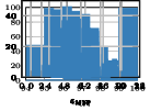
(a) $m=1$.

(b) $m=2$.

Figure 2: Relative performance $\alpha_{\textsc{opt}}$ of wip versus opt for Experiment $2$.

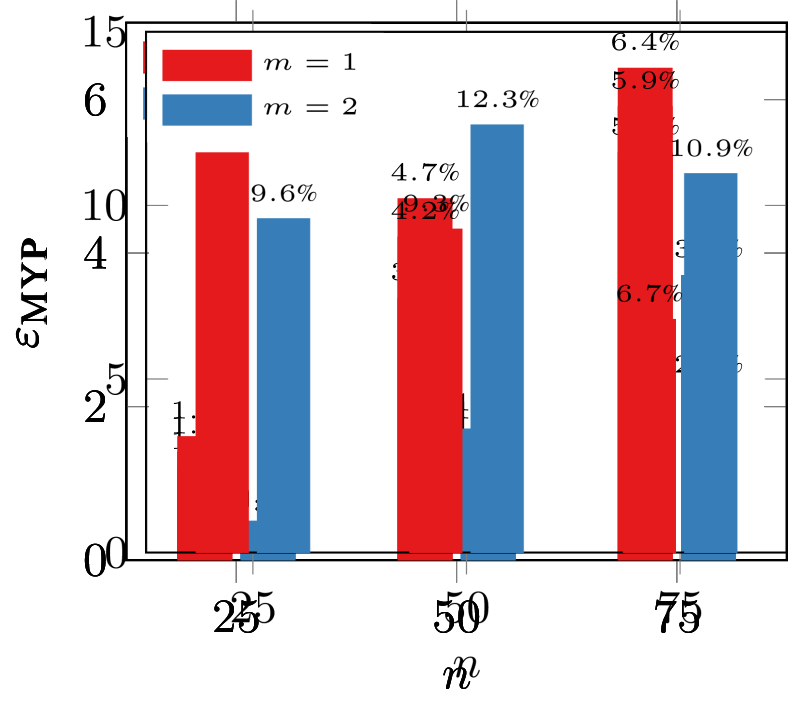
(a) $\ell=1$

(b) $\ell=2$

(c) $\ell=3$

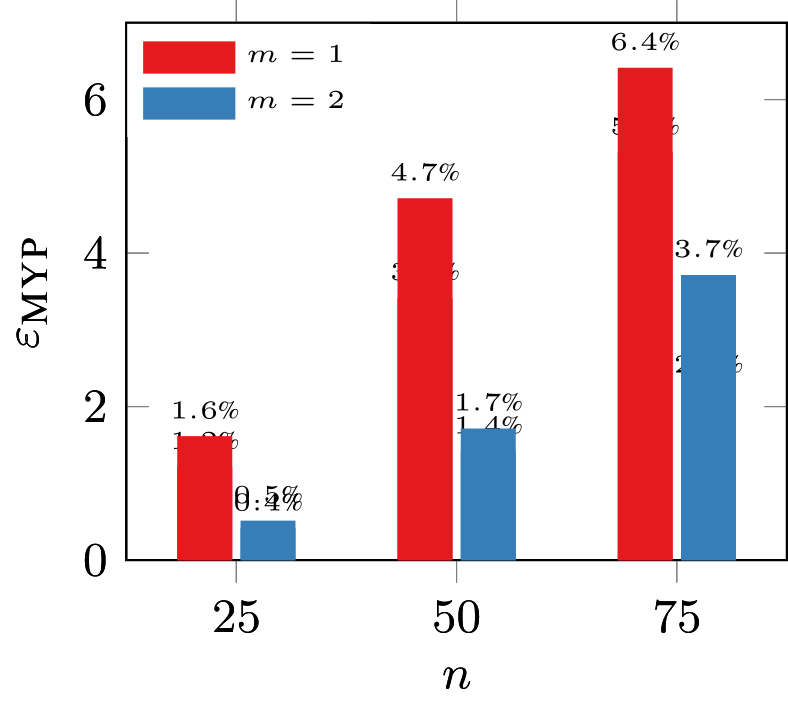
(d) $\ell=4$

Figure 3: Relative improvement $\varepsilon_{\textsc{myp}}$ of wip vs. myp for Experiment $3$.

Experiment 1) Comparison of Whittle index with the optimal policy for structured models.

The optimal policy is computed by solving the MDP for Problem 2.1, which is feasible only for small values of $|\mathcal{X}|$ and $n$. We choose $|\mathcal{X}|=5$ and $n=5$ and compare the two policies for model ${\cal P}_{\ell}(\cdot)$, $\ell\in\{1,\ldots,4\}$ and $m\in\{1,2\}$.

For a given value of $n$ and $\ell$, we pick $n$ equispaced points $(p_{1},\dots,p_{n})$ in the interval $[0.35,1]$ and choose $\mathcal{P}_{\ell}(p_{i})$ as the transition matrix of arm $i$. We observed that $\alpha_{\textsc{opt}}=J(\textsc{opt})/J(\textsc{wip})$, the relative (percentage) performance improvement of wip compared to opt, was in the range of 99.95%–100% for all parameters.

Experiment 2) Comparison of Whittle index with the optimal policy for randomly sampled models.

As before, we pick $|\mathcal{X}|=5$ and $n=5$ so that it is feasible to calculate the optimal policy. For each arm, we sample the transition matrix from ${\cal R}(5/|\mathcal{X}|)$ and repeat the experiment $250$ times. The histogram of $\alpha_{\textsc{opt}}$ over experiments for $m\in\{1,2\}$ is shown in Fig 2, which show that wip performs close to opt in all cases.

Experiment 3) Comparison of Whittle index with the myopic policy for structured models.

We generate the structured models as in Experiment $1$ but for $|\mathcal{X}|=25$, $n\in\{25,50,75\}$, and $m\in\{1,2,5\}$. In this case, let $\varepsilon_{\textsc{myp}}=(J(\text{{myp}})-J(\text{{wip}}))/J(\text{{myp}})$ denote the relative improvement of wip compared to myp. The results of $\varepsilon_{\textsc{myp}}$ for different choice of the parameters are shown in Fig 3.

In Fig 3, we observe that wip performs considerably better than myp. In addition to that, performance of wip is better with respect to myp when $\ell=4$ which is more complicated than models where $\ell\in\{1,2,3\}$. However, increasing $m$ doesn’t necessarily contribute to better $\varepsilon_{\textsc{myp}}$ as overlap between the choices of the two policies may increase. Note that as ${\cal P}_{4}(\cdot)$ is very different from the rest of the models, the trend of bars in Fig 3(d) with respect to $n$ varies differently from the rest of the models.

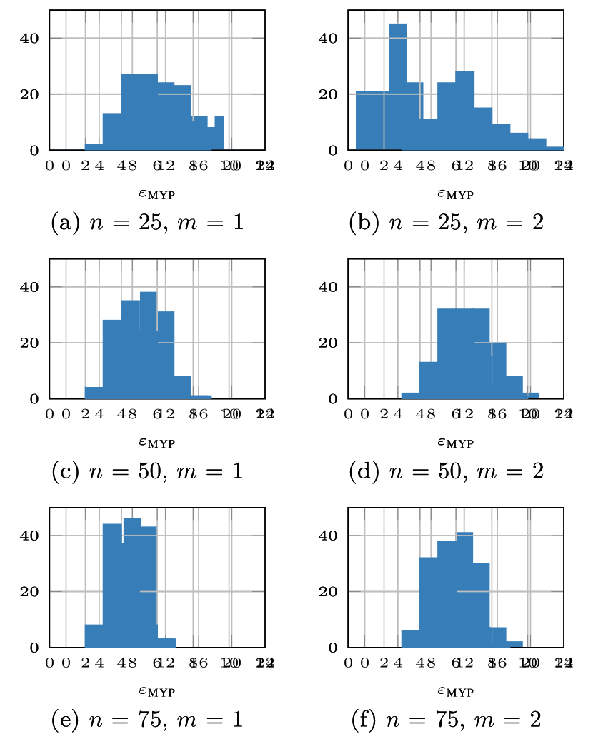
Figure 4: Relative improvement $\varepsilon_{\textsc{myp}}$ of wip vs. myp for Experiment $4$.

Figure 5: Relative improvement $\varepsilon_{\textsc{myp}}$ of wip vs. myp for Experiment $5$.

Experiment 4) Comparison of Whittle index with the myopic policy for randomly sampled models

We generate $250$ random models as described in Experiment $2$ but for $|\mathcal{X}|=25$ and larger values of $n$. For each case, $\varepsilon_{\textsc{myp}}$ is computed. The histogram of $\varepsilon_{\textsc{myp}}$ for different choices of the parameters are shown in Fig 5.

The result shows that on average, wip performs considerably better than myp and this improvement is guaranteed as the concentration of data for the sampled models is mostly on positive values of $\varepsilon_{\textsc{myp}}$.

Experiment 5) Comparison of Whittle index with the myopic policy for restart models.

We generate $250$ random stochastic matrices for $P(0)$. We set $|\mathcal{X}|=25$ and $n\in\{25,50,75\}$ and $m\in\{1,2\}$. For each case, $\varepsilon_{\textsc{myp}}$ is computed and the histogram of $\varepsilon_{\textsc{myp}}$ for different choices of the parameters is shown in Fig 5.

7 Conclusion

We present two general sufficient conditions for restless bandit processes to be indexable. The first condition depends only on the transition matrix $P(1)$ while the second condition depends on both $P(0)$ and $P(1)$. These sufficient conditions are based on alternative characterizations of the passive set, which might be useful in general as well. We also present refinements of these sufficient conditions that are simpler to verify. Two of these simpler conditions are worth highlighting: models where the active action resets the state according to a known distribution and models where the discount factor is less than $0.5$.

We then present a generalization of a previous proposed adaptive greedy algorithm, which was developed to compute the Whittle index for a sub-class of restless bandits known as PCL indexable bandits. We show that the generalized adaptive greedy algorithm computes the Whittle index for all indexable bandits. We provide a computationally efficient implementation of our algorithm, which computes the Whittle indices of a restless bandit with $K$ states in $\mathcal{O}(K^{3})$ computations.

Finally, we show how to refine the results for two classes for restless bandits: stochastic monotone bandits and restless bandits with controlled restarts. We also present a detailed numerical study which shows that Whittle index policy performs close to the optimal policy and considerably better than a myopic policy.

Appendix A Proof of Proposition 2.5

We first present a preliminary result.

Lemma A.1

For $\tau=0$, the policy $h_{0}$ satisfies $J^{(h_{0})}_{\lambda}(x)=H_{\lambda}(x,1)=(1-\beta)c(x,1)+W_{\lambda}$.

Proof A.2

Consider the stopping time $\tau=0$. The policy $h_{0},$ takes the active action at time $0$ and follows the optimal policy afterwards. Thus, for any $x\in\mathcal{X}$, $J^{(h_{0})}(x)=(1-\beta)(c(x,1)+\lambda)+\beta\sum_{y\in\mathcal{X}}P_{xy}(1)V_{\lambda}(y)=H_{\lambda}(x,1)$. By (4) and (6) we have $H_{\lambda}(x,1)=(1-\beta)c(x,1)+W_{\lambda}(x)$.

We now proceed with the proof of Proposition 2.5. By definition, $\Pi^{(a)}_{\lambda}=\Pi_{\lambda}$. We establish the equality of other characterizations.

1. $\Pi^{(a)}_{\lambda}=\Pi^{(b)}_{\lambda}$. We have $x\in\Pi_{\lambda}\overset{(a)}{\iff}g_{\lambda}(x)=0\overset{(b)}{\iff}H_{\lambda}(x,0)<H_{\lambda}(x,1)$ where $(a)$ follows from (5) and $(b)$ follows from the dynamic program (3).

2. $\Pi^{(b)}_{\lambda}\subseteq\Pi^{(c)}_{\lambda}$. Let $\sigma$ denote the hitting time of $\mathcal{X}\setminus\Pi_{\lambda}$. If we start in state $x\in\Pi^{(b)}_{\lambda}=\Pi_{\lambda}$, then the policy $h_{\sigma,\lambda}$ is same as the optimal policy. Hence, $J^{(h_{\sigma,\lambda})}_{\lambda}(x)=H_{\lambda}(x,0)$. Thus, for any $x\in\Pi^{(b)}_{\lambda}=\Pi_{\lambda}$, $J^{(h_{\sigma,\lambda})}_{\lambda}(x)=H_{\lambda}(x,0)\overset{(a)}{<}H_{\lambda}(x,1)\overset{(b)}{=}J^{(h_{0})}_{\lambda}(x)$ where $(a)$ follows from fact that $x\in\Pi^{(b)}_{\lambda}$ and $(b)$ from Lemma A.1.

3. $\Pi^{(c)}_{\lambda}\subseteq\Pi^{(b)}_{\lambda}$. Let $x\in\Pi^{(c)}_{\lambda}$ and $\sigma\in\Sigma$ denote a stopping time such that $J^{(h_{\sigma,\lambda})}_{\lambda}(x)<J^{(h_{0})}_{\lambda}(x)$. Now, the optimal policy performs at least as well as policy $h_{\sigma,\lambda}$. Therefore, $V_{\lambda}(x)\leq J^{(h_{\sigma,\lambda})}_{\lambda}(x)$. Combining this result with Lemma A.1 we have $V_{\lambda}(x)<H_{\lambda}(x,1)$. Thus, we must have $V_{\lambda}(x)=H_{\lambda}(x,0)$ which results in $H_{\lambda}(x,0)<H_{\lambda}(x,1)$ which implies $x\in\Pi^{(b)}_{\lambda}$.

4. $\Pi^{(c)}_{\lambda}=\Pi^{(d)}_{\lambda}$. According to the definitions of $L(x,\tau)$ and $W_{\lambda}(x)$ we have

   $$J^{(h_{\tau,\lambda})}_{\lambda}(x)=(1-\beta)L(x,\tau)+\mathds{E}[\beta^{\tau}W_{\lambda}(X_{\tau})|X_{0}=x].$$ (23)

   Thus, $J^{(h_{\sigma,\lambda})}_{\lambda}(x)<J^{(h_{0})}_{\lambda}(x)$ if and only if

   $$(1-\beta)L(x,\sigma)+\mathds{E}[\beta^{\sigma}W_{\lambda}(X_{\sigma})|X_{0}=x]<(1-\beta)c(x,1)+W_{\lambda}(x)$$ (24)

   where we have used (23) for $J^{(h_{\sigma,\lambda})}_{\lambda}(x)$ and Lemma A.1 for $J^{(h_{0})}_{\lambda}(x)$. Rearranging the terms of (24) we get the expression in $\Pi^{(d)}_{\lambda}$. Hence, $\Pi^{(c)}_{\lambda}=\Pi^{(d)}_{\lambda}$.

Appendix B Proof of Theorem 3.5

B.1 Proof of Theorem 3.5.a

We first present a preliminary result. Let $\Delta_{\lambda}:=\lambda^{\prime\prime}-\lambda^{\prime}$ for any

Lemma B.1

Under (11), for any $\lambda^{\prime\prime}>\lambda^{\prime}$ and $\sigma\in\Sigma$, $\sigma\neq 0$, we have that for any $x\in\mathcal{X}$,

$$W_{\lambda^{\prime}}(x)-\mathds{E}[\beta^{\sigma}W_{\lambda^{\prime}}(X_{\sigma})|X_{0}=x]\leq W_{\lambda^{\prime\prime}}(x)-\mathds{E}[\beta^{\sigma}W_{\lambda^{\prime\prime}}(X_{\sigma})|X_{0}=x],$$

Proof B.2

By (6), we have for any $x\in\mathcal{X}$,

$$(W_{\lambda^{\prime\prime}}(x)-\mathds{E}[\beta^{\sigma}W_{\lambda^{\prime\prime}}(X_{\sigma})|X_{0}=x])-(W_{\lambda^{\prime}}(x)-\mathds{E}[\beta^{\sigma}W_{\lambda^{\prime}}(X_{\sigma})|X_{0}=x])\\ =(1-\beta)\Delta_{\lambda}\bigl{(}1-M(x,\sigma)\bigr{)}+\beta\mathds{E}\biggl{[}\sum_{y\in\mathcal{X}}\bigl{(}P_{xy}(1)-\beta^{\sigma}P_{X_{\sigma}y}(1)\bigr{)}\bigl{(}V_{\lambda^{\prime\prime}}(y)-V_{\lambda^{\prime}}(y)\bigr{)}\biggm{|}X_{0}=x\biggr{]}$$ (25)

Now since $\sigma\geq 1$, $M(x,\sigma)\leq\beta$ and,

$$(1-\beta)\Delta_{\lambda}(1-M(x,\sigma))\geq\Delta_{\lambda}(1-\beta)^{2}$$ (26)

Now consider,

$$\hskip-10.00002pt\beta\mathds{E}\biggl{[}\sum_{y\in\mathcal{X}}\bigl{(}P_{xy}(1)-\beta^{\sigma}P_{X_{\sigma}y}(1)\bigr{)}\bigl{(}V_{\lambda^{\prime\prime}}(y)-V_{\lambda^{\prime}}(y)\bigr{)}\biggm{|}X_{0}=x\biggr{]}$$

$$\stackrel{{\scriptstyle(a)}}{{\geq}}\beta\mathds{E}\biggl{[}\sum_{y\in\mathcal{X}}\bigl{(}P_{xy}(1)-\beta P_{X_{\sigma}y}(1)\bigr{)}\bigl{(}V_{\lambda^{\prime\prime}}(y)-V_{\lambda^{\prime}}(y)\bigr{)}\biggm{|}X_{0}=x\biggr{]}$$

$$\stackrel{{\scriptstyle(b)}}{{\geq}}\beta\Delta_{\lambda}\mathds{E}\biggl{[}\sum_{y\in\mathcal{X}}\Bigl{\{}\bigl{[}P_{xy}(1)-\beta P_{X_{\sigma}y}(1)\bigr{]}^{+}N^{(g_{\lambda^{\prime\prime}})}(y)$$

$$\hskip 60.00009pt+\bigl{[}P_{xy}(1)-\beta P_{X_{\sigma}y}(1)\bigr{]}^{-}N^{(g_{\lambda^{\prime}})}(y)\Bigr{\}}\bigg{|}X_{0}=x\biggr{]}$$

$$\stackrel{{\scriptstyle(c)}}{{\geq}}-\Delta_{\lambda}(1-\beta)^{2},$$ (27)

where $(a)$ holds due to $\sigma\geq 1$ and $(b)$ holds by Lemma 3.3 and $(c)$ follows from (11). Substituting (26) and (27) in (25), we get the result of the Lemma.

We now proceed with the proof of Theorem 3.5a. Consider $\lambda^{\prime}<\lambda^{\prime\prime}$. Suppose $x\in\Pi_{\lambda^{\prime}}$. By Proposition 2.5.d, there exists a $\sigma\neq 0$ such that $(1-\beta)\left(L(x,\sigma)-c(x,1)\right)<W_{\lambda^{\prime}}(x)-\mathds{E}[\beta^{\sigma}W_{\lambda^{\prime}}(X_{\sigma})|X_{0}=x].$ Combining this result with the result of Lemma B.1, we infer $(1-\beta)\left(L(x,\sigma)-c(x,1)\right)<W_{\lambda^{\prime\prime}}(x)-\mathds{E}[\beta^{\sigma}W_{\lambda^{\prime\prime}}(X_{\sigma})|X_{0}=x].$ Thus, $x\in\Pi_{\lambda^{\prime\prime}}$. Hence, $\Pi_{\lambda^{\prime}}\subseteq\Pi_{\lambda^{\prime\prime}}$ and the RB is indexable.

B.2 Proof of Theorem 3.5.b

Consider $\lambda^{\prime}<\lambda^{\prime\prime}$. A RB is indexable if $\Pi_{\lambda^{\prime}}\subseteq\Pi_{\lambda^{\prime\prime}}$ or equivalently, for any $x$ such that $H_{\lambda^{\prime}}(x,0)<H_{\lambda^{\prime}}(x,1)$ then $H_{\lambda^{\prime\prime}}(x,0)<H_{\lambda^{\prime\prime}}(x,1)$. A sufficient condition for that is to show that $H_{\lambda^{\prime}}(x,1)-H_{\lambda^{\prime}}(x,0)\leq H_{\lambda^{\prime\prime}}(x,1)-H_{\lambda^{\prime\prime}}(x,0)$, or equivalently, show that $H_{\lambda^{\prime\prime}}(x,0)-H_{\lambda^{\prime}}(x,0)\leq H_{\lambda^{\prime\prime}}(x,1)-H_{\lambda^{\prime}}(x,1)$. We prove this inequality as follows.

Let $\Delta_{\lambda}=\lambda^{\prime\prime}-\lambda^{\prime}$. By (4), we have for any $x\in\mathcal{X}$,

$$\hskip-10.00002pt\left(H_{\lambda^{\prime\prime}}(x,1)-H_{\lambda^{\prime}}(x,1)\right)-\left(H_{\lambda^{\prime\prime}}(x,0)-H_{\lambda^{\prime}}(x,0)\right)$$

$$=\Delta_{\lambda}(1-\beta)+\beta\sum_{y\in\mathcal{X}}(P_{xy}(1)-P_{xy}(0))(V_{\lambda^{\prime\prime}}(y)-V_{\lambda^{\prime}}(y))$$

$$\stackrel{{\scriptstyle(a)}}{{\geq}}\Delta_{\lambda}\Bigl{(}1-\beta+\beta\sum_{y\in\mathcal{X}}\left[P_{xy}(1)-P_{xy}(0)\right]^{+}N^{(g_{\lambda^{\prime\prime}})}(y)+\left[P_{xy}(1)-P_{xy}(0)\right]^{-}N^{(g_{\lambda^{\prime}})}(y)\Bigr{)}\stackrel{{\scriptstyle(b)}}{{\geq}}0$$

where $(a)$ follows from Lemma 3.3 and $(b)$ holds by (12). Therefore the RB is indexable.

Appendix C Proof of Proposition 3.6

We prove the result of each part separately.

1. This follows from observing that

   $$\hskip-10.00002pt\sum_{y\in\mathcal{X}}\Bigl{\{}\bigl{[}\beta P_{zy}(1)-P_{xy}(1)\bigr{]}^{+}N^{(g)}(y)-\bigl{[}P_{xy}(1)-\beta P_{zy}(1)\bigr{]}^{+}N^{(h)}(y)\Bigr{\}}$$

   $$\stackrel{{\scriptstyle(a)}}{{\leq}}\sum_{y\in\mathcal{X}}\bigl{[}\beta P_{zy}(1)-P_{xy}(1)\bigr{]}^{+}N^{(g)}(y)$$

   $$\stackrel{{\scriptstyle(b)}}{{\leq}}\sum_{y\in\mathcal{X}}\bigl{[}\beta P_{zy}(1)-P_{xy}(1)\bigr{]}^{+}\leq\max_{x,z\in\mathcal{X}}\sum_{y\in\mathcal{X}}\bigl{[}\beta P_{zy}(1)-P_{xy}(1)\bigr{]}^{+}$$

   where we are ignoring negative terms in $(a)$ and using $N^{(g)}(x)\leq 1$ in $(b)$.

2. For any $x,y,z\in\mathcal{X}$, $P_{xy}(1)-\beta P_{zy}(1)=(1-\beta)P_{xy}(1)$. Thus,

   $$\hskip-10.00002pt\sum_{y\in\mathcal{X}}\Bigl{\{}\bigl{[}\beta P_{zy}(1)-P_{xy}(1)\bigr{]}^{+}N^{(g)}(y)-\bigl{[}P_{xy}(1)-\beta P_{zy}(1)\bigr{]}^{+}N^{(h)}(y)\Bigr{\}}$$

   $$=-\sum_{y\in\mathcal{X}}(1-\beta)P_{xy}(1)N^{(h)}(y)\leq 0<\frac{(1-\beta)^{2}}{\beta}.$$

3. This follows from observing that

   $$\hskip-10.00002pt\sum_{y\in\mathcal{X}}\Bigl{\{}\bigl{[}P_{xy}(0)-P_{xy}(1)\bigr{]}^{+}N^{(g)}(y)-\bigl{[}P_{xy}(1)-P_{xy}(0)\bigr{]}^{+}N^{(h)}(y)\Bigr{\}}$$

   $$\stackrel{{\scriptstyle(a)}}{{\leq}}\sum_{y\in\mathcal{X}}\bigl{[}P_{xy}(0)-P_{xy}(1)\bigr{]}^{+}N^{(g)}(y)$$

   $$\stackrel{{\scriptstyle(b)}}{{\leq}}\sum_{y\in\mathcal{X}}\bigl{[}P_{xy}(0)-P_{xy}(1)\bigr{]}^{+}\leq\max_{x\in\mathcal{X}}\sum_{y\in\mathcal{X}}\bigl{[}P_{xy}(0)-P_{xy}(1)\bigr{]}^{+}$$

   where we are ignoring negative terms in $(a)$ and using $N^{(g)}(x)\leq 1$ in $(b)$.

4. $\beta\leq 0.5$ implies that

   $$\dfrac{1-\beta}{\beta}\geq 1\geq\max_{x\in\mathcal{X}}\bigl{[}P_{xy}(0)-P_{xy}(1)\bigr{]}^{+}$$

   which is the same as sufficient condition (c) established above.

Appendix D Proof of Lemma 4.1

The proof of each part is as follows:

1. Since the model is indexable and $y\in\Gamma_{d+1}$, $w(d)=\lambda_{d+1}$. Therefore, the optimal policy is indifferent between choosing the active and the passive action at $\lambda=\lambda_{d+1}$.

2. By definition, for any $\lambda\in(\lambda_{d},\lambda_{d+1}]$, $h_{d}$ is an optimal policy. Therefore, we have $J^{({h}_{d,y})}_{\lambda}(x)\geq J^{(h_{d})}_{\lambda}(x)$ with $y\in{\cal X}\backslash{\cal P}_{d}$, for all $x\in{\cal X}$ with equality if $y\in\Gamma_{d+1}$ and $\lambda=\lambda_{d+1}$.

References

• [1] Abad, C. and Iyengar, G. (2016). A near-optimal maintenance policy for automated DR devices. 7, 1411–1419.
• [2] Akbarzadeh, N. and Mahajan, A. (2019). Dynamic spectrum access under partial observations: A restless bandit approach. In Canadian Workshop on Information Theory. IEEE. pp. 1–6.
• [3] Akbarzadeh, N. and Mahajan, A. (2019). Restless bandits with controlled restarts: Indexability and computation of whittle index. In Conf. Decision Control. pp. 7294–7300.
• [4] Ansell, P. S., Glazebrook, K. D., Niño-Mora, J. and O’Keeffe, M. (2003). Whittle’s index policy for a multi-class queueing system with convex holding costs. Math. Operat. Res. 57, 21–39.
• [5] Archibald, T. W., Black, D. P. and Glazebrook, K. D. (2009). Indexability and index heuristics for a simple class of inventory routing problems. Operat. Res. 57, 314–326.
• [6] Avrachenkov, K., Ayesta, U., Doncel, J. and Jacko, P. (2013). Congestion control of TCP flows in internet routers by means of index policy. Computer Networks 57, 3463–3478.
• [7] Ayesta, U., Erausquin, M. and Jacko, P. (2010). A modeling framework for optimizing the flow-level scheduling with time-varying channels. Performance Evaluation 67, 1014–1029.
• [8] Bertsimas, D. and Niño-Mora, J. (1996). Conservation laws, extended polymatroids and multiarmed bandit problems; a polyhedral approach to indexable systems. Math. Operat. Res. 21, 257–306.
• [9] Chakravorty, J. and Mahajan, A. (2014). Multi-armed bandits, gittins index, and its calculation. Methods and applications of statistics in clinical trials: Planning, analysis, and inferential methods 2, 416–435.
• [10] Deo, S., Iravani, S., Jiang, T., Smilowitz, K. and Samuelson, S. (2013). Improving health outcomes through better capacity allocation in a community-based chronic care model. Operat. Res. 61, 1277–1294.
• [11] Egidi, N. and Maponi, P. (2006). A Sherman–Morrison approach to the solution of linear systems. Journal of computational and applied mathematics 189, 703–718.
• [12] Feinberg, E. A. and He, G. (2020). Complexity bounds for approximately solving discounted MDPs by value iterations. Operations Research Letters 48, 543–548.
• [13] Gittins, J., Glazebrook, K. and Weber, R. (2011). Multi-armed bandit allocation indices. John Wiley & Sons.
• [14] Gittins, J. C. (1979). Bandit processes and dynamic allocation indices. Journal of the Royal Statistical Society. Series B 148–177.
• [15] Glazebrook, K., Hodge, D. and Kirkbride, C. (2013). Monotone policies and indexability for bidirectional restless bandits. Adv. Appl. Prob. 45, 51–85.
• [16] Glazebrook, K. and Mitchell, H. (2002). An index policy for a stochastic scheduling model with improving/deteriorating jobs. Naval Research Logistics 49, 706–721.
• [17] Glazebrook, K. D., Kirkbride, C. and Ouenniche, J. (2009). Index policies for the admission control and routing of impatient customers to heterogeneous service stations. Operat. Res. 57, 975–989.
• [18] Glazebrook, K. D., Mitchell, H. M. and Ansell, P. S. (2005). Index policies for the maintenance of a collection of machines by a set of repairmen. Euro. J. Operat. Res. 165, 267–284.
• [19] Glazebrook, K. D., Ruiz-Hernandez, D. and Kirkbride, C. (2006). Some indexable families of restless bandit problems. Adv. Appl. Prob. 38, 643–672.
• [20] Jacko, P. (2012). Optimal index rules for single resource allocation to stochastic dynamic competitors. In Conf. Perf. Eval. Method. Tools. ACM.
• [21] Liu, K. and Zhao, Q. (2010). Indexability of restless bandit problems and optimality of whittle index for dynamic multichannel access. 56, 5547–5567.
• [22] Lott, C. and Teneketzis, D. (2000). On the optimality of an index rule in multichannel allocation for single-hop mobile networks with multiple service classes. Probability in the Engineering and Informational Sciences 14, 259–297.
• [23] Niño-Mora, J. (2001). Restless bandits, partial conservation laws and indexability. Adv. Appl. Prob. 33, 76–98.
• [24] Nino-Mora, J. (2002). Dynamic allocation indices for restless projects and queueing admission control: a polyhedral approach. Mathematical programming 93, 361–413.
• [25] Niño-Mora, J. (2007). Dynamic priority allocation via restless bandit marginal productivity indices. TOP 15, 161–198.
• [26] Niño-Mora, J. (2006). Restless bandit marginal productivity indices, diminishing returns, and optimal control of make-to-order/make-to-stock M/G/1 queues. Math. Operat. Res. 31, 50–84.
• [27] Papadimitriou, C. H. and Tsitsiklis, J. N. (1999). The complexity of optimal queuing network control. Math. Operat. Res. 24, 293–305.
• [28] Puterman, M. L. (2014). Markov decision processes: discrete stochastic dynamic programming. John Wiley & Sons.
• [29] Qian, Y., Zhang, C., Krishnamachari, B. and Tambe, M. (2016). Restless poachers: Handling exploration-exploitation tradeoffs in security domains. In Int. Conf. on Autonomous Agents & Multiagent Systems. pp. 123–131.
• [30] Wang, J., Ren, X., Mo, Y. and Shi, L. (2020). Whittle index policy for dynamic multichannel allocation in remote state estimation. IEEE Transactions on Automatic Control 65, 591–603.
• [31] Weber, R. R. and Weiss, G. (1990). On an index policy for restless bandits. J. Appl. Prob. 27, 637–648.
• [32] Whittle, P. (1988). Restless bandits: Activity allocation in a changing world. J. Appl. Prob. 25, 287–298.
• [33] Yu, Z., Xu, Y. and Tong, L. (2018). Deadline scheduling as restless bandits. 63, 2343–2358.