Optically-Thin Spatially-Resolved Mg ii Emission Maps the Escape of Ionizing Photons

Abstract

Early star-forming galaxies produced copious ionizing photons. A fraction of these photons escaped gas within galaxies to reionize the entire Universe. This escape fraction is crucial for determining how the Universe became reionized, but the neutral intergalactic medium precludes direct measurement of the escape fraction at high-redshifts. Indirect estimates of the escape fraction must describe how the Universe was reionized. Here, we present new Keck Cosmic Web Imager spatially-resolved spectroscopy of the resonant Mg ii 2800 Å doublet from a redshift 0.36 galaxy, J1503+3644, with a previously observed escape fraction of 6%. The Mg ii emission has a similar spatial extent as the stellar continuum, and each of the Mg ii doublet lines are well-fit by single Gaussians. The Mg ii is optically thin. The intrinsic flux ratio of the red and blue Mg ii emission line doublet, $R=F_{2796}/F_{2803}$, is set by atomic physics to be two, but Mg⁺ gas along the line of sight decreases $R$ proportional to the Mg ii optical depth. Combined with the metallicity, $R$ estimates the neutral gas column density. The observed $R$ ranges across the galaxy from 0.8-2.7, implying a factor of 2 spatial variation of the relative escape fraction. All of the ionizing photons that escape J1503+3644 pass through regions of high $R$. We combine the Mg ii emission and dust attenuation to accurately estimate the absolute escape fractions for ten local Lyman Continuum emitting galaxies and suggest that Mg ii can predict escape fraction within the Epoch of Reionization.

1 Introduction

At redshifts between 6–10 the first galaxies emitted a sufficient number of photons with $\lambda<912$ (or Lyman Continuum, LyC, photons) to reionize all of the neutral hydrogen between galaxies in the Universe (Becker et al., 2001; Fan et al., 2006; Bañados et al., 2018). This "Epoch of Reionization" (EoR) marked the first time that galaxies exerted their influence over the entire Universe. However, observations have not established how galaxies reionized the universe because the sources of ionizing photons from within these first galaxies are, at the moment, observationally unconstrained.

The two major sources of ionizing photons are massive stars and accretion onto black holes (Active Galactic Nuclei or AGN). The total emissivity ($j_{\text{ion}}$[photon s^-1 Mpc^-3]) of either AGN or star-forming galaxies can be observationally estimated as the product of their FUV luminosity function ($\rho_{\text{UV}}$[erg s^-1 Hz^-1 Mpc^-3]), the intrinsic production of ionizing photons per FUV luminosity for each source ($\xi_{\text{ion}}$[photon erg^-1 Hz]), and the fraction of ionizing photons that escape a galaxy (the escape fraction; $f_{\text{esc}}$$\left({\rm LyC}\right)$). Numerically, this is

$$j_{\text{ion}}=\text{$f_{\text{esc}}$$\left({\rm LyC}\right)$}\xi_{\text{ion}}\rho_{\text{UV}}.$$ (1)

If $f_{\text{esc}}$$\left({\rm LyC}\right)$, $\xi_{\text{ion}}$, and $\rho_{\rm UV}$ can all be measured then observations can determine $j_{\text{ion}}$ of both star-forming galaxies and AGN within the EoR. A direct comparison to the cosmological matter density, with an assumption about the clumpiness of the early Universe, determines whether a given source produces sufficient ionizing photons to reionize the Universe. High-redshift AGN are an appealing source of ionizing photons because their high-ionization and high-luminosity means that $f_{\text{esc}}$$\left({\rm LyC}\right)$ $\approx 100$%. However, current observations find too few AGN (low $\rho_{\text{UV}}$) to reionize the Universe (Hopkins et al., 2008; Willott et al., 2010; Ricci et al., 2017; Onoue et al., 2017; Matsuoka et al., 2018; Shen et al., 2020), but there may be numerous unobserved, low-luminosity AGN (Giallongo et al., 2015; Grazian et al., 2016; Matsuoka et al., 2019).

Meanwhile, vigorously star-forming galaxies must also have large reservoirs of cold neutral gas. Neutral gas efficiently absorbs ionizing photons, reducing the number of ionizing photons that escape a typical star-forming galaxy. As such $f_{\text{esc}}$$\left({\rm LyC}\right)$ is often observed to be less than 5% in the local Universe (Grimes et al., 2009; Vanzella et al., 2010; Leitherer et al., 2016; Naidu et al., 2018). However, models using typical estimates of $\xi_{\rm ion}$ and $\rho_{\text{UV}}$ indicate that $f_{\text{esc}}$$\left({\rm LyC}\right)$ must be $>$5-20% for star-forming galaxies to reionize the universe (Ouchi et al., 2009b; Robertson et al., 2013; Robertson et al., 2015; Finkelstein et al., 2019; Naidu et al., 2020). These escape values are only found in the most extreme local galaxies (Leitet et al., 2011; Borthakur et al., 2014; Izotov et al., 2016b, a; Izotov et al., 2018a; Izotov et al., 2018b).

Recently, there has been tremendous success in directly measuring $f_{\text{esc}}$$\left({\rm LyC}\right)$ from extremely compact, high-ionization, star-forming galaxies (Leitet et al., 2011; Borthakur et al., 2014; Izotov et al., 2016a, b; Vanzella et al., 2016; Shapley et al., 2016; Izotov et al., 2018a; Izotov et al., 2018b; Steidel et al., 2018; Fletcher et al., 2019; Rivera-Thorsen et al., 2019; Wang et al., 2019), demonstrating that star-forming galaxies can emit ionizing photons. The physical parameters of the recently discovered local emitters of ionizing photons ( low stellar mass, high specific star formation rate SFR/M_∗, compact, low-metallicity, and low dust attenuation) are similar to the expected properties of the first galaxies (Schaerer & de Barros, 2010). However, it is challenging to be certain whether low-redshift galaxies are actually analogs to EoR galaxies. Direct observations of $f_{\text{esc}}$$\left({\rm LyC}\right)$ must determine the sources of reionization.

Direct observations of $f_{\text{esc}}$$\left({\rm LyC}\right)$ above $z\sim 4$ are statistically unlikely because the neutral intergalactic medium (IGM) surrounding these galaxies efficiently absorbs LyC photons (Worseck et al., 2014). This high IGM opacity means that we will not directly observe the LyC of star-forming galaxies during the EoR. A major goal for the upcoming James Webb Space Telescope (JWST) is to determine the sources of cosmic reionization, but to accomplish this requires indirect methods to determine $f_{\text{esc}}$$\left({\rm LyC}\right)$.

The two major sinks of ionizing photons are photoelectric absorption by neutral hydrogen and dust; both can remove similar amounts of ionizing photons (Chisholm et al., 2018). Ideal indirect $f_{\text{esc}}$$\left({\rm LyC}\right)$ methods must be: unaffected by the high-redshift neutral IGM, bright enough to be observed at high-redshift, and trace H⁰ column density variations between 10^16-17.2 cm^-2 where H⁰ becomes optically thin to the ionizing continuum. There are currently a number of prospects of indirect indicators of ionizing photon escape (Heckman et al., 2011; Alexandroff et al., 2015; Verhamme et al., 2006; Henry et al., 2015; Chisholm et al., 2018; Henry et al., 2018; Steidel et al., 2018; McKinney et al., 2019; Berg et al., 2019). However, each has their own drawbacks: Ly$\alpha$ is bright but the neutral IGM can absorb a large portion of the Ly$\alpha$ profile at high-redshifts (Verhamme et al., 2017); the Lyman Series absorption lines are within the Ly$\alpha$ forest at high-redshift and are challenging to disentangle from foreground IGM absorption; and metal-absorption lines require deep observations to detect the stellar continuum (Steidel et al., 2018; Chisholm et al., 2018; Jaskot et al., 2019).

The ionization state of the strong Mg ii 2800 Å doublet overlaps with H⁰ ( the Mg ii ionization potential is 15 eV), such that Mg ii emission traces neutral gas and may be an ideal indirect indicator of $f_{\text{esc}}$$\left({\rm LyC}\right)$ (Henry et al., 2018). Depending on the metallicity of the intervening gas, H⁰ gas column densities $N_{\rm H^{0}}<10^{17}$ cm^-2 lead to optically thin Mg ii absorption profiles (see Section 6). Thus, the absence of Mg ii absorption suggests a neutral gas column density low enough to transmit ionizing photons. Further, Mg ii emission of low-metallicity galaxies can be 10-60% of the observed H$\beta$ flux (Guseva et al., 2013), indicating that Mg ii emission may be sufficiently bright to observe with upcoming facilities in the distant universe. Thus, Mg ii emission may help determine the sources of cosmic reionization.

Here, we present new spatially-resolved spectroscopic observations of the Mg ii 2796, 2803 Å doublet from a previously-confirmed LyC emitter, J1503+3644 (Izotov et al., 2016a). We use these observations to explore the neutral gas properties within this source of ionizing photons and test whether Mg ii emission traces the escape of ionizing photons. The outline of the paper is as follows: Section 2 describes the data reduction and analysis. We then explore the spatially integrated (Section 3) and spatially resolved (Section 4) Mg ii emission line properties. The physical implications of the spatial distribution and kinematics of the Mg ii emission and neutral gas is discussed in Section 5. Section 6 explores the relationship between the Mg ii emission and the neutral gas column densities that we use in Section 7 to indirectly infer the $f_{\text{esc}}\left(\text{Mg\,{ii}}\right)$ and $f_{\text{esc}}$$\left({\rm LyC}\right)$. Section 7.4 describes the future prospects to detect Mg ii at high-redshift to determine the sources of cosmic reionization.

2 DATA

Table 1: Properties of J1503 from Izotov et al. (2016a). The first row gives the redshift, the second row gives the logarithm of the stellar mass, the third row gives the O⁺⁺ temperature, the forth row gives the electron density, the fifth row gives the nebular metallicity determined from the [O iii] 4363 Å line (using the T_e method), the sixth and seventh row give the H$\beta$ and [O iii] 5007 Å restframe equivalent width, and the eighth row gives the [O iii] 5007 Å to [O ii] 3727 Å flux ratio.

Property	Value
z	0.3557
log(M∗/M⊙)	8.22
T(O iii)	14850 K
ne	280 cm-3
12+log(O/H)	7.95
H$\beta$ Equivalent width	297 Å
$[$O iii$]$ 5007 Equivalent width	1403Å
$F$[O iii] 5007 / $F$[O ii] 3727	4.9

2.1 Observations and Data Reduction

We selected SDSS J150342.83+364450.75 (hereafter J1503; Izotov et al., 2016a) because the galaxy has the largest Mg ii 2800 Å emission flux from public Sloan Digital Sky Survey (SDSS) observations (Alam et al., 2015) in the Izotov et al. (2016a) LyC emitting sample. At $z=0.3557$, the Mg ii 2800Å doublet is observed at wavelengths of 3789.90 and 3799.63Å, respectively, within the wavelength range of the blue sensitive Integral Field Spectrograph Keck Cosmic Web Imager (KCWI) on the Keck ii telescope (Morrissey et al., 2018). KCWI is an image slicer that is highly optimized to measure faint diffuse emission, and ideally suited to map the extended Mg ii structure in J1503.

KCWI is highly configurable and contains an array of beam-slicers and gratings. The different configurations trade off between field of view, wavelength coverage, spatial sampling, and spectral resolution. J1503 is a compact star-forming galaxy that is unresolved by the SDSS and NUV imaging (Izotov et al., 2016a), thus a large field of view is not as important as spatial sampling. Similarly, we are predominately interested in spectrally resolving the Mg ii lines. Thus, we used the small image-slicer, the BM grating with a central wavelength of 4000 Å, and 1x1 binning to afford a field of view of 8.4″ $\times$ 20.4″, a spatial sampling of 0.35″ perpendicular to the slice direction (seeing limited along the slice direction), a full restframe wavelength coverage of 2700–3300 Å, and a spectral resolution of R $=8000$ (37 km s^-1).

On the night of January 31^st 2019, we obtained a total of 65 on-source minutes (3900 s) using an AABB dither pattern with a dither separation of 1″and an average airmass of 1.07. The individual exposures were processed through the standard KCWI KDERP pipeline Version 1.1.0 (Morrissey et al., 2018). The eight major steps of this reduction include: (1) bias, over-scan, and cosmic ray removal, (2) dark and scattered light subtraction; (3) geometric transformation and wavelength calibration using a ThAr arc lamp in each image slice with a mean RMS scatter of the calibration emission of 0.042 Å about the reference values, below the expected 0.2Å for the BM grating; (4) flat fielding each slice by creating a master-flat using 6 dome flats; (5) standard sky subtraction, (6) collapsing the individual slices into spatial intensity and variance cubes in air wavelengths; (7) a differential atmospheric refraction correction based upon the observed airmass of J1503; and (8) flux calibrating the J1503 observations using the standard star BD+26 2606. Below, we provide additional specifics for a few of these steps.

We used the standard sky subtraction which uses a B-spline to generate a 2-dimensional sky model. Emission from astronomical objects within the field of view were excluded using a 1$\sigma$ clipping. Since J1503 is small on the sky (Figure 1), the 8.4″ $\times$ 20.4″field of view contains a sufficient amount of emission-free regions to accurately model the sky emission. We tested whether providing a mask around the galaxy before creating the sky model improved the sky-subtraction, but we found negligible differences. After the sky-subtraction, we checked multiple regions within the 2-D data cube for sky over-subtraction and did not find any such indication.

The four individual reduced exposures were shifted into the reference frame of the first exposure and the three subsequent exposures were combined with an inverse variance weighting. With the small slicer and 1x1 binning, the spatial-pixels (spaxels) in the resultant data cubes have sizes that are 0.35″$\times$0.147″ in the Right Ascension and Declination directions. This leads to the rectangular pixels shown in the spatial plots.

Immediately after the J1503 science observations, we observed the standard star BD+26 2606. This blue A5V star is one of the KWCI standard stars and is sufficiently blue to flux calibrate the observed wavelengths. We ran the KCWI pipeline in interactive mode, setting the standard star fitting regions by hand to minimize the residuals, while paying special attention to mask out the stellar Balmer absorption features and sky emission lines. The final inverse sensitivity curves were inspected to ensure continuity and proper fits to the stellar continuum. Finally, the total spatially-integrated, flux-calibrated spectrum of J1503 was compared to the SDSS spectrum. We found a factor of 1.4 difference in the total flux, but the overall spectral shape of the KCWI observations nicely matched the SDSS spectrum. Also, the relative wavelength calibration was excellent between the two spectra, such that the Mg ii emission peaks were consistent within the spectral resolution. The spatially integrated KCWI spectrum was multiplied by a factor of 1.4 to align with the SDSS to complete the flux calibration. Only the relative fluxing of the KCWI observations matter because we only use observables within the KCWI observations which have the same flux calibration.

In the spectral dimension, we corrected the observed frame spectra for foreground Milky Way reddening using the Cardelli et al. (1989) attenuation curve and the reddening value of E(B-V) = 0.013 from Green et al. (2015). We then shifted the spectrum into the restframe of the galaxy, $\lambda_{\rm rest}=\lambda_{\rm obs}/(1+z)$, using $z=0.3557$ as measured from the SDSS spectrum (Izotov et al., 2016a).

We subtracted the continuum from the spatial cube using the Common Astronomy Software Applications (casa; McMullin et al., 2007) routine imcontsub, using a first order polynomial. We tested different orders and found that orders higher than 1 produced similar results. For the Mg ii emission region, we fit the continuum in spectral regions that, by eye, avoided two [Fe iv] emission lines at 2829.4 and 2835.7 Å, respectively, and Mg i 2852 Å. The continuum was fit at $\lambda_{\rm rest}=2766-2791$ Å and $\lambda_{\rm rest}=2808-2825$ Å (see blue regions in Figure 2). Similarly, we fit a first-order polynomial between restframe wavelengths of 3171–3182 Å and 3194–3200 Å for the He i 3188 Å line to avoid possible contributions from the weakly detected He ii 3202 Å line. This produced wavelength-calibrated, flux-calibrated, continuum-subtracted cubes from which we analyzed the data.

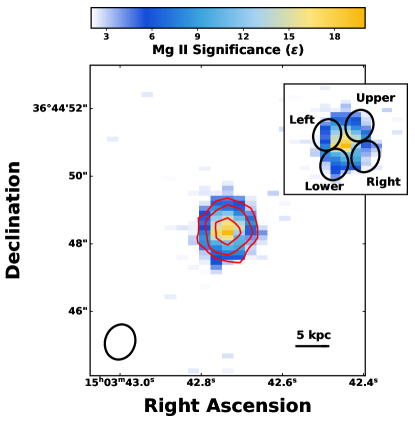
Figure 1: Spatial map of the integrated, continuum-subtracted Mg ii emission (the 2796 plus the 2803 Å transitions) from J1503, in units of the Mg ii statistical significance: $\epsilon=1.5\times 10^{-18}$ erg s^-1 cm^-2 per spaxel. Red contours are the 2, 5, and 10 $\epsilon$ contours of the stellar continuum with $\epsilon_{\rm s}=1.4\times 10^{-19}$erg s^-1 cm^-2 Å^-1 per spaxel. The measured 1.04″$\times$ 0.92″ seeing, from the standard star observation, is given by the black circle in the lower left. A scale bar is given in the lower right and this figure is a 9″$\times$9″cutout of the full 8.4″$\times$20.4″ KCWI field of view. The inset shows the location of the four spatial distinct apertures used in Table 3.

To quantify the observed spatial resolution, we fit the size of the standard star, BD+26 2606, in the KCWI cubes using the casa two-dimensional fitting tool at the same wavelength as the Mg ii emission ($\lambda_{\rm obs}\approx 3790$ Å). We measured the size of the standard star to be $1.04\pm 0.01$″$~{}\times~{}0.92\pm 0.01$″ at 177^∘. This is consistent with the 1-1.2″ seeing reported by the DIMM seeing at the telescope that remained relatively stable during the observations. A single slice width in this configuration is 0.35″, such that there are at least 2.6 spaxels per seeing PSF. We find a similar standard star size for the spectral region near the He i 3188 Å line. We use this as our spatial resolution and denote it as a black circle in the bottom left of our spatial plots (e.g., Figure 1).

We also compare the KCWI observed-frame optical spectrum to the HST/COS G160M (Green et al., 2012) far-ultraviolet spectrum of J1503 (HST project ID: 13744, PI: Thuan; Izotov et al., 2016a; Verhamme et al., 2017). We downloaded the data from MAST and extracted the spectrum following the methods outlined in Worseck et al. (2016) that carefully consider the pulse-heights of the extraction region to optimize the extraction of faint objects. The G160M data have nominal spectral resolution of 20 km s^-1, similar to the KCWI observations.

2.2 Line Profile Fitting

We calculated the inferred Mg ii emission line properties in two ways. The first method used the casa immoments routine to create continuum-subtracted Mg ii 2800 Å and He i 3188 Å integrated intensity maps. For the Mg ii integrated intensity map, we integrated over both of the Mg ii emission lines to boost the signal-to-noise ratio (Figure 1). We also obtained a continuum image of each spaxel using the imsubcont casa routine, which compares the spatial extent of the stellar continuum and the emission lines (red contours in Figure 1). We calculated the error ($\epsilon$) of the integrated intensity maps by taking the standard deviation of off-source regions within the integrated intensity maps. The integrated Mg ii map has $\epsilon=1.5\times 10^{-18}$ erg s^-1 cm^-2 per spaxel and the continuum map has $1.4\times 10^{-19}$erg s^-1 cm^-2 Å^-1 per spaxel (or $\sim 23$ mag arcsec^-2 in the U-band).

Secondly, we fit the emission lines in each spaxel using single Gaussian profiles. As discussed in Section 6, the non-trivial observation that the Mg ii emission lines are well-fit by single Gaussians indicates the lack of resonant absorption and scattering. We fit for the velocity offset ($v$) from zero-velocity as established by the SDSS redshift, total velocity width ($\sigma_{\text{tot}}$), continuum flux (F_cont), and total integrated flux ($F$) of each Gaussian profile as

$$G(\lambda)=\frac{F}{\sqrt{2\pi}\sigma_{\rm tot}}e^{-\frac{v^{2}}{2\sigma_{\text{tot}}^{2}}}+F_{\rm cont}.$$ (2)

The intrinsic velocity width, $\sigma_{\text{int}}$, of each emission line is determined from $\sigma_{\text{tot}}$ by subtracting the instrumental broadening of 37 km s^-1  in quadrature (i.e., $\sigma_{\text{tot}}^{2}=\sigma_{\rm int}^{2}+\sigma_{\rm inst}^{2}$). We take the Mg ii restframe wavelengths in air, $\lambda_{0}=$ 2795.528 and 2802.704 Å, from the NIST database (Kramida et al., 2018) to establish the restframe wavelength of each Mg ii emission line. We fit for $v$, $\sigma$, $F_{\rm cont}$, and $F$ using the Levenberg-Marquardt linear-least squares fitting routine mpfit (Markwardt, 2009). The properties ($v$, $\sigma$, $F$) of the 2796 Å and 2803 Å Mg ii emission lines were fit independently, but simultaneously, to allow for the properties to vary distinctly from transition-to-transition (see Section 6). We also fit the He i 2945 Å and He i 3188 Å profiles with single Gaussians. This spaxel-by-spaxel fitting enables the determination of the emission properties at each spatial location. Whenever we plot the Mg ii properties, we only include spaxels that have a signal-to-noise ratio (S/N) greater than 2 for the Mg ii emission line ratio ($F_{2796}/F_{2803}$).

3 Spatially integrated Mg ii emission

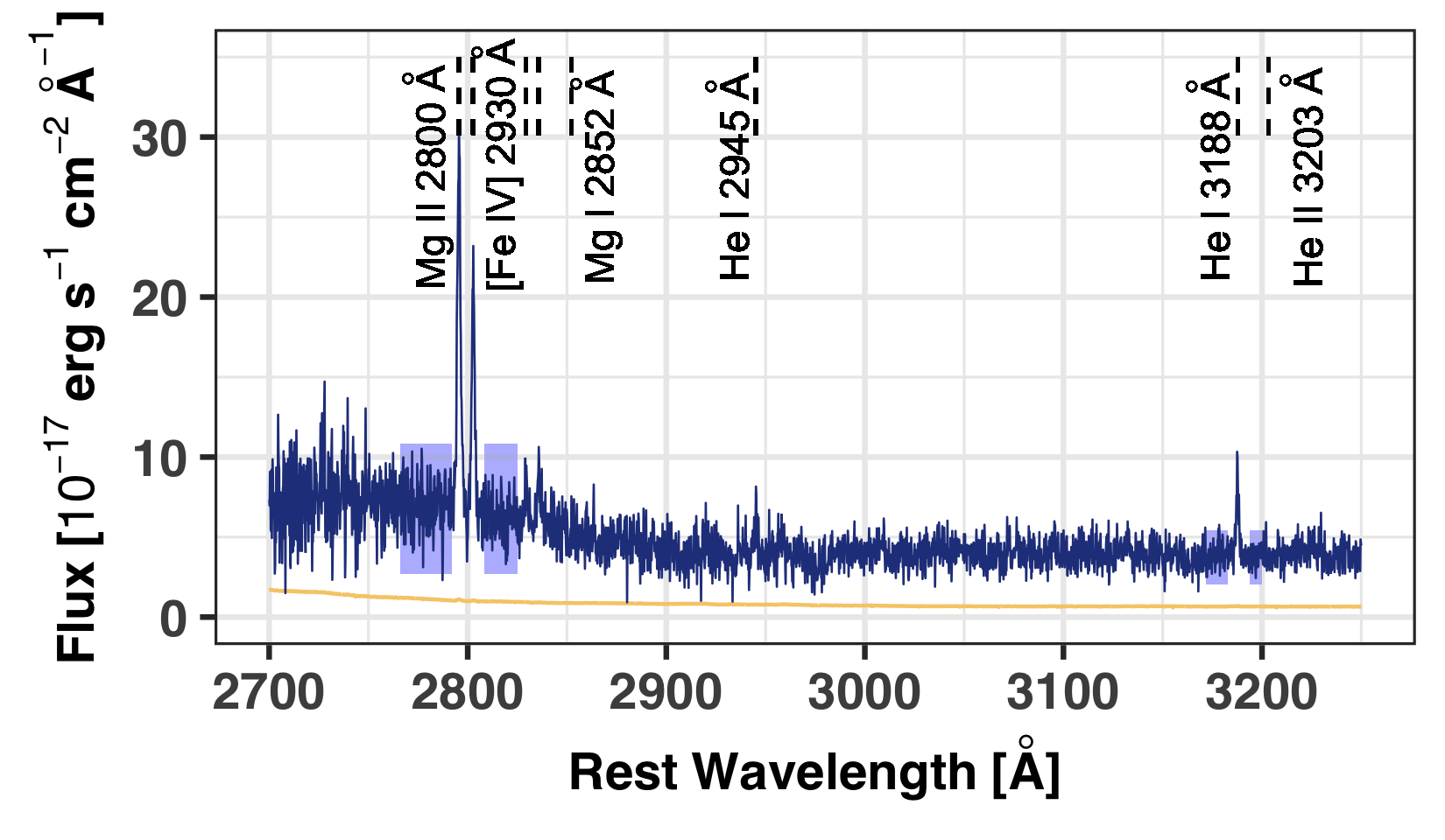
Figure 2: The spatially-integrated restframe spectrum extracted from a 3.0″ diameter region centered on the bright emission peak in Figure 1. The gold line shows the extracted 1$\sigma$ error on the flux. Emission lines are labelled above the spectrum. Strong Mg ii 2796, 2803 Å and He i 3188 Å, along with weak [Fe iv] 2829, 2836 Å and He i 2945 Å, emission lines are detected. We do not detect Mg i absorption at any significance. The shaded blue regions are the regions used to subtract the continuum from the spectrum.

Figure 2 shows the integrated spectrum extracted from an aperture with a 3″diameter centered on the brightest emission peak from J1503. Even though integrating removes spatial information, summing the spaxels produces a high S/N spectrum of the galaxy (the Mg ii 2796 Å line is detected at the 21$\sigma$ significance) that is comparable to previous SDSS and HST observations. Figure 2 shows a strong Mg ii 2800 Å doublet along with moderately strong He i 3188 Å recombination emission. Among the weaker lines, the high S/N spectrum also shows a weak [Fe iv] 2830 Å doublet, He i 2945 Å, and He ii 3202 Å lines. Notably absent from the spectrum is the Mg i 2852 Å absorption line. This contrasts with galaxies with strong Mg ii absorption, which often also have strong Mg i absorption (Tremonti et al., 2007; Weiner et al., 2009; Martin et al., 2012; Rubin et al., 2014; Finley et al., 2017). Mg i has an ionization potential of 7.6 eV; the non-detection indicates that there is negligible gas in lower ionization states than Mg ii in J1503 (see Section 6).

The overall spatially-integrated Mg ii emission flux is comparable to the SDSS flux. Using the same internal extinction correction as Izotov et al. (2016a) ($E(B-V)$ = 0.09), we find a total observed Mg ii 2796 Å flux of $8.5\pm 0.4\times 10^{-16}$ erg s^-1 cm^-2 while Izotov et al. (2016a) measured $9\pm 1\times 10^{-16}$ erg s^-1 cm^-2. To put the strength of these Mg ii lines into perspective: the integrated extinction-corrected Mg ii 2796+2803 Å emission is 40, 53, and 8$\%$ of the SDSS [O ii] 3727 Å, H$\beta$, and [O iii] 5007 Å fluxes, respectively.

Figure 3 shows the single Gaussian fit to the continuum subtracted Mg ii doublet from the spatially-integrated profile. The single Gaussian fits match the observed Mg ii profile. We do not observe any absorption signatures nor do we find strong line profile asymmetries typical of radiatively scattered resonant emission lines (Verhamme et al., 2006; Prochaska et al., 2011; Verhamme et al., 2015; Scarlata & Panagia, 2015; Orlitová et al., 2018; Kakiichi & Gronke, 2019). This is especially apparent in the weaker Mg ii 2803 Å. The Mg ii 2796 Å profile has a slight emission excess at the highest positive velocities ($\sim+200$ km s^-1). However, the slight emission excess is only statistically discrepant from the fits at the 2$\sigma$ significance level for two pixels (20 km s^-1 ), less than the spectral resolution. On a whole, the fit residuals of 89.6% (86 of 96) and 99.0% (95 of 96) of the pixels in the Mg ii region are less than 2$\sigma$ and 3$\sigma$ discrepant, respectively, in agreement with the expectation of a Gaussian distribution. Therefore, all observed deviations from the fit are fully consistent within the noise of the observations.

The fitted Gaussian parameters, listed in Table 2, further describe the relative shapes of the line profiles. The stronger Mg ii 2796 Å line is broader than the Mg ii 2803 Å line at 2.5$\sigma$ significance, but both are centered at zero velocity. These Mg ii emission line characteristics are not necessarily true for all observed Mg ii profiles. Henry et al. (2018) observed 10 Green Pea galaxies (9 currently without available LyC observations), and all of those Mg ii profiles were offset to the red from zero velocity. Some of those galaxies also have asymmetric profiles and most are not well-fit by a single Gaussian. Unlike the Gaussian Mg ii profiles of J1503, the Mg ii profiles from Henry et al. (2018) are heavily modified by resonant scattering.

Table 2: The fitted properties of the emission lines from the 3.0″ in diameter spatially-integrated region from J1503+3644. The second column is the velocity offset of the emission lines from the SDSS redshift ($v$), the third column is the spectral-resolution-corrected intrinsic velocity width ($\sigma_{\text{int}}$), and the last column is the total integrated flux of the emission line (flux-corrected to match the SDSS flux values). The fluxes have been corrected for Milky Way attenuation. No internal attenuation correction has been made.

Line	$v$	$\sigma_{\text{int}}$	Integrated flux
	[km s-1]	[km s-1]	[10-16 erg s-1 cm-2]
Mg ii 2796Å	$4\pm 4$	$91\pm 2$	$6.4\pm 0.3$
Mg ii 2803Å	$7\pm 4$	$78\pm 3$	$3.7\pm 0.3$
He i 3188Å	$-10\pm 5$	$57\pm 5$	$1.0\pm 0.2$
Mg ii Doublet Flux Ratio	$1.7\pm 0.1$

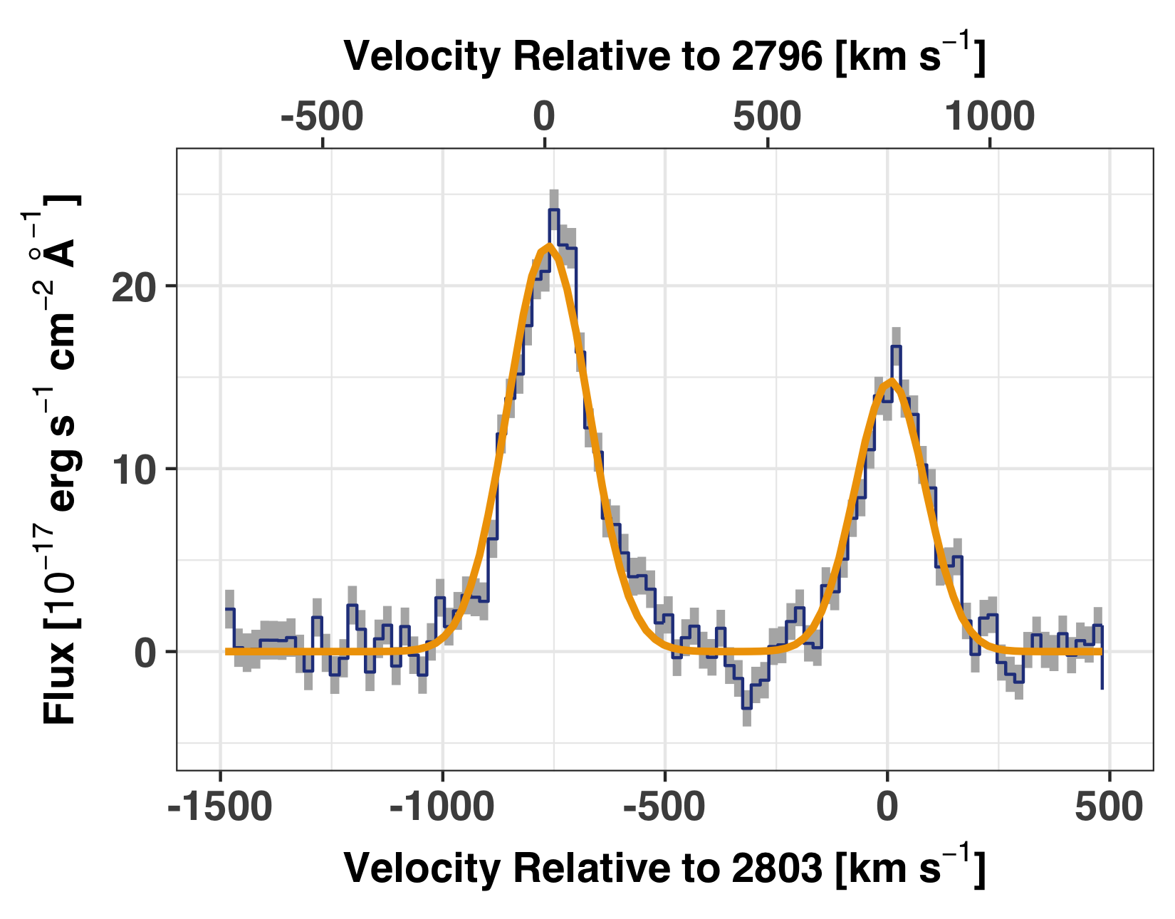
Figure 3: Zoom-in on the spatially integrated, continuum-subtracted Mg ii 2796, 2803 Å doublet (blue) with a gray ribbon showing the 1$\sigma$ error on the flux. The lower x-axis shows the velocity relative to the Mg ii 2803 Å line (the right emission line) and the upper x-axis shows the velocity relative to the Mg ii 2796 Å line (the left emission line). The gold line shows a single Gaussian fit to each Mg ii emission line. Both Mg ii emission lines are within 2$\sigma$ of zero velocity, relative to the optical emission lines from the SDSS spectra (which has a 5 km s^-1  redshift error), and well fit by a single Gaussian.

Finally, in Section 6, we use the Mg ii doublet flux ratio to constrain the optical depth of the Mg ii gas. We define the doublet flux ratio as

$$R=\frac{F_{2796}}{F_{2803}},$$ (3)

where we measure $R=1.7\pm 0.1$ in the spatially integrated spectrum.

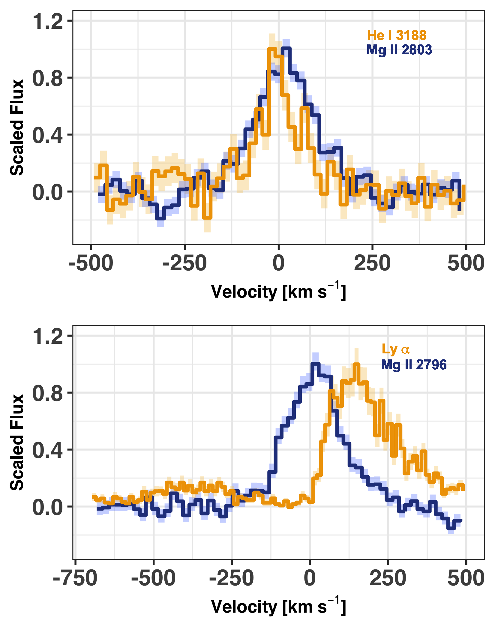
Figure 4: Comparison of the Mg ii emission lines (blue) to the nebular He i 3188 Å (upper panel) and Ly$\alpha$ from HST/COS observations (lower panel). Each profile is normalized by the peak flux of the emission line. The 1$\sigma$ errors are shown by a lighter ribbon of the same color. The red portion of the Mg ii emission is slightly broader than the He i emission. The Mg ii does not resemble the Ly$\alpha$ emission.

We compare the spatially-integrated Mg ii  2803 Å  to the nebular emission line He i 3188 Å in the top panel of Figure 4. We compare to the 2803 Å transition because it has a lower $f$-value than the 2796 Å transition, and is, thus, a better comparison to the He i line. With an intrinsic line width of $\sigma_{\text{int}}=57\pm 5$ km s^-1, the He i is spectrally resolved, but narrower than the Mg ii 2803 Å line at 2.6$\sigma$ significance. The two line profiles are fairly consistent over the blue portion of their profiles, while they diverge slightly in the red portion. Conversely, the moderate-resolution HST/COS G160M Ly$\alpha$ profile in the bottom panel of Figure 4 has a very different profile shape from the Mg ii 2796 Å emission line. Through the metallicity, there is a factor of $\sim$10⁵ larger neutral hydrogen column density than Mg⁺ column density, such that Ly$\alpha$ is more strongly impacted by resonant scattering (Neufeld, 1990; Dijkstra et al., 2006; Verhamme et al., 2006; Gronke et al., 2015; Kakiichi & Gronke, 2019; Michel-Dansac et al., 2020). Radiative transfer effects are seen in the shape of the Ly$\alpha$ profile from J1503: the main emission peak is redshifted by $+140$ km s^-1  from line center, while a weak blue peak is $-290$ km s^-1  from line center (Verhamme et al., 2017). Meanwhile, the Mg ii emission does not show these radiative transfer effects: it is centered at zero-velocity and well-fit by a single Gaussian profile.

In summary, the spatially-integrated Mg ii emission-line profiles are well-fit by single Gaussians that are centered at zero velocity (Figure 3). The fairly symmetric Mg ii line profiles resemble slightly broader versions of the nebular He i profiles and are markedly different from the double-peaked Ly$\alpha$ profiles (Figure 4). Importantly, the flux ratio of the Mg ii doublet lines is $R=1.7\pm 0.1$. This ratio will be discussed fully in Section 6.

4 Spatially resolved Mg II emission

Here we explore the Mg ii properties on a spaxel-by-spaxel basis. The main goal of this analysis is to determine the spatial extent of the Mg ii emission (Section 4.1) and the variation of the Mg ii properties (Section 4.2), with special attention paid to $R$, the doublet flux ratio (Section 4.3). $R$ encodes information on the Mg ii optical depth (Section 6) and the fraction of Mg ii (and LyC) emission that escapes J1503 (see Section 7.1).

4.1 The Spatial Extent of Mg ii Emission

Mg ii emission, in Figure 1, is extended beyond the 1.04″$\times$0.92″ seeing disk (compare the contours to the black circle in the bottom). We fit a 2-dimensional profile to the continuum subtracted Mg ii profile and measure a FHWM of $1.32\pm 0.04$″$\times 1.21\pm 0.04$″ at 175^∘. In comparison, the nebular He i 3188 Å in Figure 5 is not spatially extended, although it does peak at the same location as the Mg ii emission. Note that the nebular He i emission is faint and the peak of the emission is only detected at the 5$\sigma$ significance level, substantially less than the 21 $\epsilon$ of the Mg ii 2796 Å emission. Additionally, we do not detect any statistically significant Mg i – in absorption or emission – in any of the integrated spectra or individual spaxels.

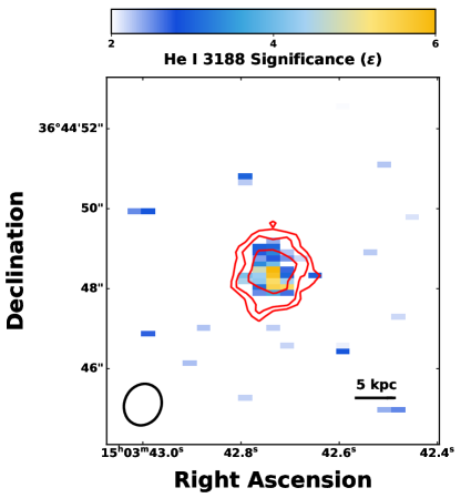
Figure 5: Spatial map of the integrated continuum-subtracted He i 3188Å emission, in units of the He i significance: $\epsilon=5.8\times 10^{-19}$ erg s^-1 cm^-2 per spaxel. The measured 1.04″ $\times$ 0.92″ seeing is given by the black circle in the lower left, and a 1.0″ scale bar is given in the lower right (with the projected physical size of 1.0″ at $z=0.3557$). The red contours are the 3, 5, and 10$\epsilon$ integrated Mg ii emission contours. These contours are not the same as in Figure 1. The He i and Mg ii emission are both centered in the same location.

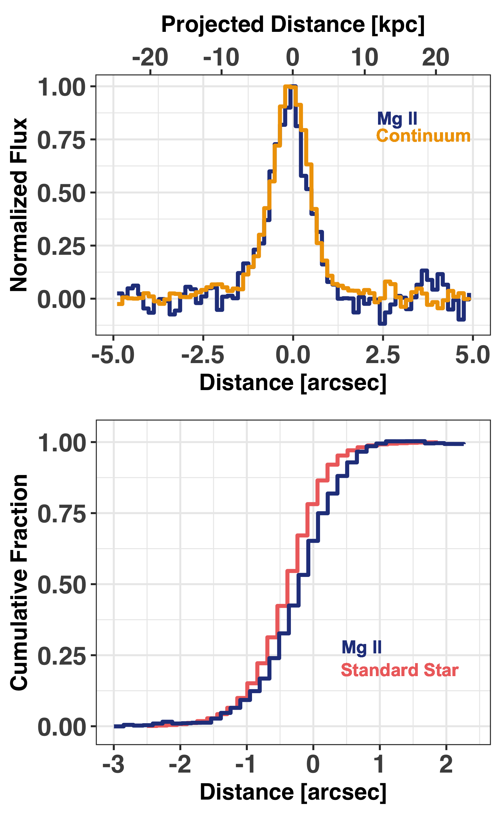
Figure 6: Upper Panel: The surface brightness profiles of the continuum-subtracted Mg ii 2796+2803 Å emission (from Figure 1; blue line) and the stellar continuum (gold line). Both surface brightness profiles are extracted from the same vertical line through the brightest Mg ii emission spaxel. The Mg ii and stellar continuum have similar light profiles. The upper x-axis shows the projected physical size at $z=0.3557$. Lower Panel: The cumulative distribution of the continuum-subtracted Mg ii emission. The pink line compares the Mg ii cumulative distribution to the standard star cumulative distribution. While the Mg ii is slightly spatially extended, the 3.0″diameter SDSS fibers captures all of the Mg ii emission.

Table 3: Fitted emission line properties of four spatially distinct regions within the KCWI observations. Each spectrum was extracted from a region with size equal to the measured seeing, separated from the brightest emission peak, and distinct from the other three regions ( see the inset in Figure 1). The first column gives the region location relative to the main Mg ii emission peak, the second and third columns give the fitted intrinsic velocity width, corrected for the spectral resolution ($\sigma_{\text{int}}$), of the Mg ii 2803 Å and Mg ii 2796 Å lines, respectively. The forth column is the doublet ratio $R=F_{2796}/F_{2803}$. The fifth column gives the inferred column density of neutral hydrogen and column six gives the resultant relative escape fraction. The relative escape fraction is calculated using the Mg ii flux ratio and the ISM metallicity, but ignores the effects of dust attenuation (see Equation 23).

Region	$\sigma_{2803}$	$\sigma_{2796}$	$R$	$N_{\mathrm{H^{0}}}$	$f_{\rm esc}^{\rm rel}$
	[km s-1]	[km s-1]		[1016 cm-2]	[%]
Left	$79\pm 3$	$108\pm 2$	$1.5\pm 0.2$	$6\pm 3$	$69\pm 13$
Right	$80\pm 3$	$81\pm 2$	$1.7\pm 0.2$	$3\pm 2$	$83\pm 10$
Upper	$85\pm 4$	$108\pm 3$	$1.8\pm 0.2$	$2\pm 2$	$88\pm 10$
Lower	$65\pm 3$	$96\pm 3$	$2.1\pm 0.3$	$<2$	$>88$

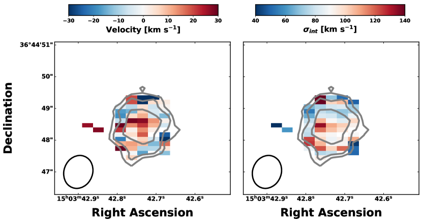
Figure 7: Left Panel: The spatial distribution of the fitted Mg ii 2796 Å velocity centroid. There is no obvious coherent velocity distribution and the mean velocity of the individual spaxels is $3\pm 15$ km s^-1 . Right Panel: The spatial distribution of the estimated intrinsic velocity width ($\sigma_{\text{int}}$) of the Mg ii 2796 Å emission line. The gray contours are the 2, 5, and 10$\epsilon$ significance levels of the integrated Mg ii emission. The 1.04″$\times$ 0.92″ seeing disk is included in the lower left of each panel.

The red contours in Figure 1 demonstrate that the stellar continuum closely follows the shape of the Mg ii emission. To better quantify the spatial relation between the Mg ii and the stellar continuum, Figure 6 shows their surface brightness profiles. The Mg ii emission peaks at the same location as the stellar continuum, both have similar FWHMs, and both are roughly symmetric. Both the Mg ii and stellar continuum are concentrated within a projected physical distance of $\pm 5$ kpc. The cumulative Mg ii flux distribution, shown in the bottom panel of Figure 6, illustrates that the Mg ii is highly centrally concentrated, but is slightly extended beyond the 1.04″$\times$ 0.92″ seeing disk of the standard star (pink line).

4.2 Spatially-resolved Emission Properties

Using the spaxel-by-spaxel emission line fits, we can explore the spatial variation of the Mg ii emission. Large-scale galactic outflows from compact galaxies have been observed with Mg ii emission out to 100 kpc (Rubin et al., 2014; Rupke et al., 2019; Burchett et al., 2020). Similarly, if the gas within J1503 rotates then we would expect to observe coherent spatial velocity gradients (Micheva et al., 2019). We do not find strong spatial variations in the Mg ii 2796 Å velocity (left panel of Figure 7, the 2803 Å velocity does not show spatial trends either). The Mg ii emission does not show signatures of coherent rotation nor ordered structure. The Mg ii velocities range between $-31$ and $+46$ with a median of $3\pm 15$ km s^-1. Similarly, the right panel of Figure 7 shows the Mg ii 2796 Å intrinsic velocity width ($\sigma_{2796}$), measured to have a mean value of $88\pm 24$ km s^-1. The median $v$ and $\sigma_{\rm int}$ values from all of the spaxels are similar to the values determined by fitting the spatially-integrated profile (Table 2). This indicates that the spatially-integrated value is representative of the median spaxel-by-spaxel values.

The final parameter that we study spatially is the Mg ii doublet flux ratio, $R=F_{2796}/F_{2803}$. As described below, $R$ traces the Mg ii optical depth and the spatially-resolved emission maps the Mg⁺ column density distribution. The left panel of Figure 8 shows that $R$ varies from 0.8 to 2.7 with a median of $1.7\pm 0.4$. The median value of the spatial distribution agrees with the value measured from the integrated profile. To test the seeing impact and spatially correlated noise on the $R$ distribution, the right panel of Figure 8 shows the $R$ distribution convolved with a 2-dimensional Gaussian that has the same parameters as the fitted seeing. While edge effects of the convolution make the outer regions appear at lower $R$ than physical, there are distinct $R$ variations in the inner regions of J1503. Even smoothed to the seeing resolution, there is significant structure in the observed $R$ values.

Figure 9 shows the Mg ii profiles for two spatially-distinct spaxels within J1503. The Mg ii emission line profiles change from spaxel-to-spaxel, and equivalently from location-to-location, within the galaxy. The Mg ii 2803 Å line has similar strength in both spaxels, but the Mg ii 2796 Å is stronger for the blue profile. This leads to $R=2$ for the blue profile and $R=1.3$ for the gold profile. Figure 10 compresses the individual spaxels from the spatial $R$ map of Figure 8 into a histogram. The median value, the dashed gray line, splits the distribution in half, but the distribution does not peak there. Rather, the $R$ distribution is broad with a possible slight double-peaked distribution: one near $R=2$ and one near $R=1.5$. However, the median measured error on individual pixels is 0.3, precluding a definitive confirmation of this morphology. Thus, this distribution could be equally-well explained as a uniform distribution.

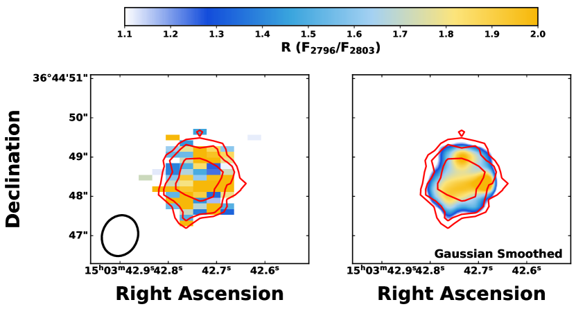
Figure 8: Left Panel: Spatial map of the Mg ii doublet flux ratio, $R=F_{2796}/F_{2803}$. There is spatial variation: the upper left regions have lower $R$ values on average than the lower right regions. The contours show the 2, 5, and 10$\epsilon$ flux levels of the integrated Mg ii emission. The 1.04″$\times$ 0.92″ seeing disk is included as a circle in the lower left. Right Panel: The same $R$ spatial map as in the left, but convolved with a Gaussian the size of the seeing disk. Note that edge effects artificially cause the outer regions to appear to have lower $R$ values.

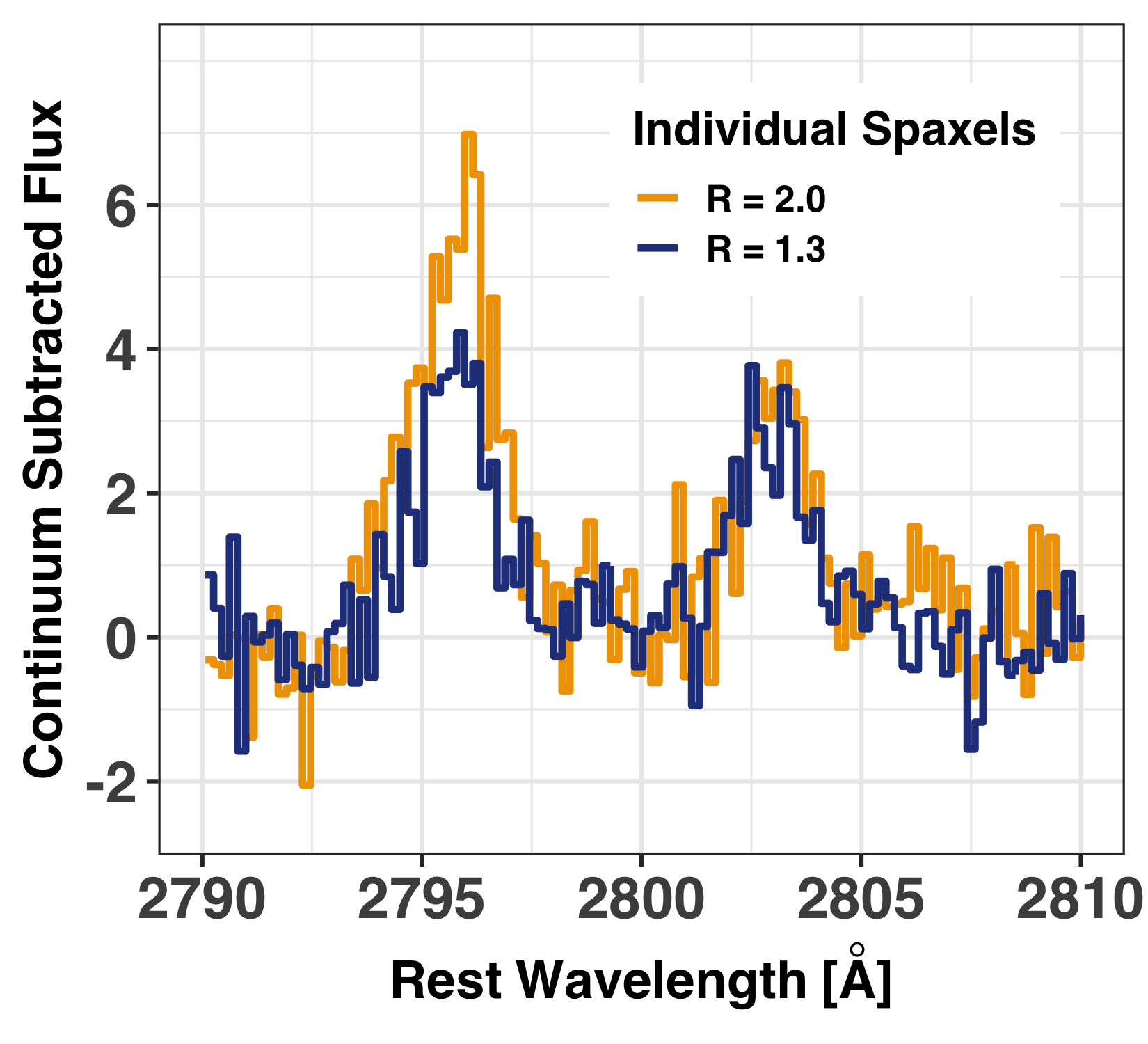
Figure 9: Two individual spaxel s separated by more than the seeing. Each spaxel shows a different flux ratio of the 2796 and 2803 Å emission feature ($R=F_{2796}/F_{2803}$). These two individual spatial locations within the galaxy have different $R$ values: $2.0\pm 0.3$ ( gold) and $1.3\pm 0.3$ ( blue).

To further explore the impact of spatial resolution and seeing on the spatial variation of $R$, we extracted four spectra from regions with an aperture size equal to the seeing disk and spatially distinct from each other. These regions are above, below, to the left, and to the right of the bright Mg ii peak in Figure 1, but do not include the peak. Fitting these four spatially distinct regions finds that the lower and the left quadrants have the largest $R$ differences of $2.1\pm 0.3$ and $1.5\pm 0.2$, respectively (see Table 3). This is seen in both panels of Figure 8: the lower portion is largely gold, while the spaxels in the left quadrant are largely blue.

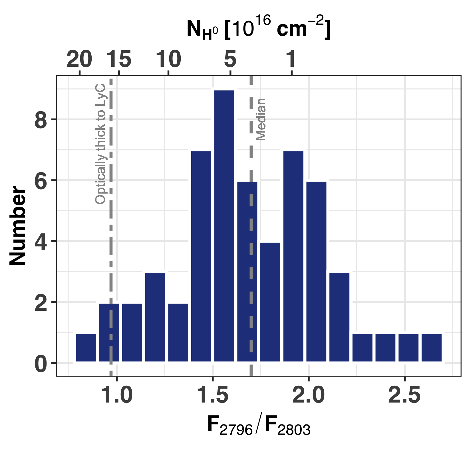
Figure 10: Histogram of the Mg ii flux ratio, $R=F_{2796}/F_{2803}$, for all of the S/N $>2$ spaxels within J1503. High $R$ regions imply lower H⁰ column densities, as marked by the upper x-axis, assuming the gas-phase metallicity of J1503 and a constant dust depletion (see Equation 15). The dashed line marks the median of the $R$ distribution (1.7) and the dot-dashed line is the column density where H⁰ becomes optically thick to ionizing photons. Note that the typical per spaxel uncertainty on $R$ is 0.3 (two bins), and the distribution could be uniformly distributed. Spaxels with $R>2$ have large errors such that they are statistically consistent with 2.

4.3 Averaging Based on the Doublet Ratio

In Section 6 and Section 7, we emphasize the utility of $R$ to determine the Mg⁺ and H⁰ optical depths and column densities. To explore the relation between the Mg ii emission lines and optical depth at high S/N, we determine the average spectra of high and low $R$ regions by averaging all individual spaxels with a measured $R>1.7$ and all spaxels with $R<1.7$. We call these averaged spectra the High and Low $R$ spectra, respectively.

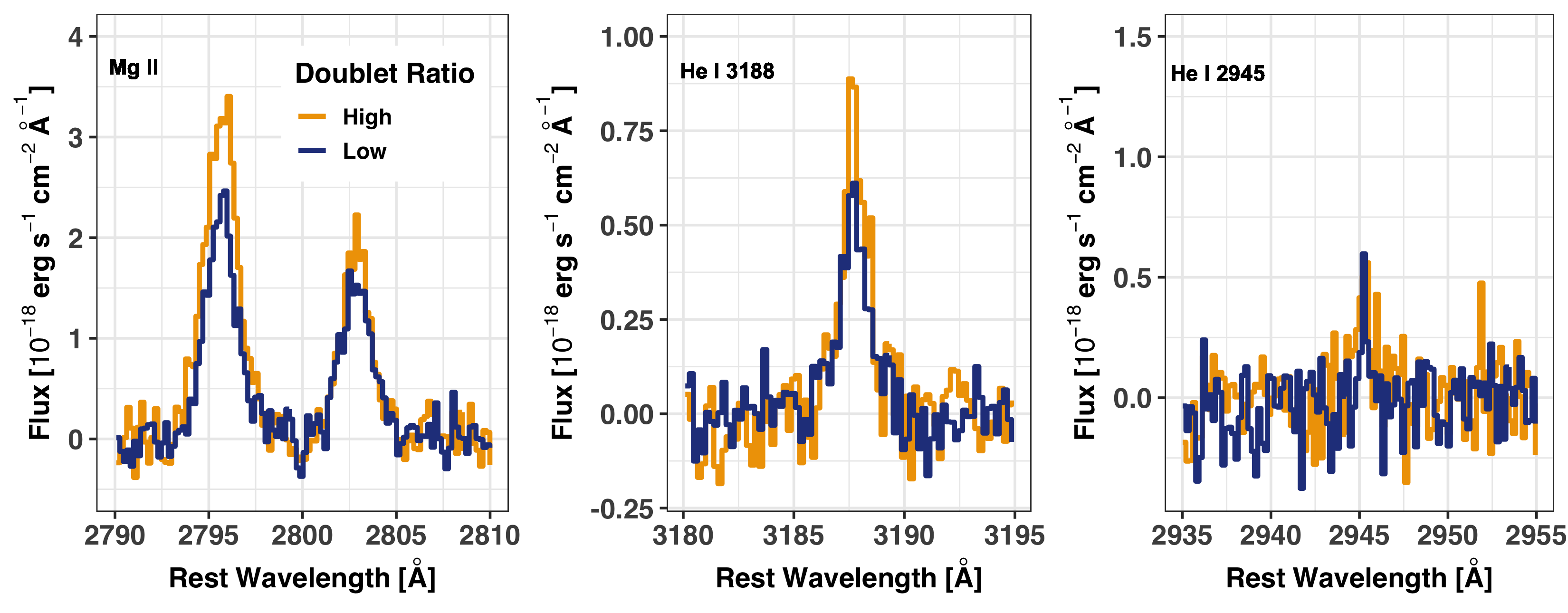
Figure 11: Mean continuum subtracted emission profiles of all spaxels split based upon whether the Mg ii 2796 to 2803Å flux ratio ($R=F_{2796}/F_{2803}$) is greater than 1.7 (High; blue line) or less than 1.7 (Low; gold line). The three panels are different nebular emission lines: Mg ii, He i 3188 Å, and He i 2945Å (from left to right). High $R$ spaxels have a stronger Mg ii 2796 Å integrated flux, but nearly the same Mg ii 2803 Å flux. The High $R$ composite also has marginally stronger He i 3188 Å emission.

The left panel of Figure 11 shows the mean Mg ii emission line profiles of the High (blue) and Low (gold) $R$ regions. The Mg ii emission properties, listed in Table 4, show statistical variation between the two composites. By construction, the High $R$ composite has $R$ values that are consistent with 2, while the Low $R$ composite is 1.43. In the Low $R$ composite, the 2803 and 2796 Å line widths are statistically similar, while the 2796 Å line is significantly broader than the 2803 Å line in regions with High $R$. We do not observe statistically significant differences in the Mg ii velocity centroids.

The middle and right panels of Figure 11 show two He i emission lines, 3188 and 2945 Å, respectively. He i 3188 Å is strongly detected in both composites, with the Low $R$ having weaker average He i than the High $R$ composite. The He i 2945 Å line is weak in both composites, but moderately stronger in the High $R$ composite.

Table 4: Fitted line profile properties of two composites of individual spaxels below (Low $R$; Column 2) and above (High $R$; Column 3) the median $R$ value of 1.7. Parameters above the second horizontal line are derived from the Mg ii profiles, while parameters below it are derived using a combination of the Mg ii, the He i 3188 Å, and the He i 2945 Å emission lines (the He i emission flux ratio, the gas-phase attenuation, the inferred relative escape fraction, and the inferred absolute escape fraction).

Property	Low $R$	High $R$
v2796 [km s-1]	$6\pm 4$	$6\pm 4$
v2803 [km s-1]	$9\pm 4$	$7\pm 4$
$\sigma_{2796}$ [km s-1]	$90\pm 3$	$97\pm 4$
$\sigma_{2803}$ [km s-1]	$95\pm 3$	$82\pm 4$
F2796/F2803	$1.43\pm 0.07$	$1.96\pm 0.08$
F3188/F2945	$4.26\pm 1.07$	$2.17\pm 0.30$
E$($B-V$)$ [mag]	3	0.13
$f_{\rm esc}^{\rm rel}$(LyC)	$63\pm 4$	$97\pm 6$
$f_{\text{esc}}$$\left({\rm LyC}\right)$	0	19

5 Neutral gas within and surrounding a galaxy that emits ionizing photons

The Mg ii emission from J1503 is not spatially extended beyond the stellar continuum and is centrally concentrated with a FWHM of 1.32″ $\times$ 1.21″ (6–6.6 kpc in physical units; Figure 1), considerably smaller than the KCWI field of view of 8.4″ $\times$ 20.4″. As shown in Section 6, Mg ii emission is closely connected to the neutral gas properties in the galaxy. The combination of the small spatial distribution and the relationship between Mg ii and neutral gas implies that the bulk of the dense metal-bearing neutral gas is not extended beyond the 13 kpc of the stellar continuum (Figure 6). Since ionizing photons are observed to escape from this galaxy, it is perhaps not surprising that the circum-galactic medium of J1503 is devoid of neutral hydrogen: there must be a paucity of gas along the line-of-sight for ionizing photons to escape.

However, a diminished neutral hydrogen circum-galactic medium is in stark contrast to galaxies observed at moderate (Steidel et al., 2011; Östlin et al., 2014; Hayes et al., 2014; Cantalupo et al., 2014; Erb et al., 2018; Cai et al., 2019) and high-redshift (Ouchi et al., 2009a; Sobral et al., 2015) with Ly$\alpha$ emission. At $z\sim 3$, studies find Ly$\alpha$ halos around Lyman Break Galaxies that are upwards of 15 times larger than the stellar continuum (Steidel et al., 2011; Wisotzki et al., 2016). Some of these galaxies have since been confirmed to emit ionizing photons (Steidel et al., 2018). However, these galaxies are either more massive or more spatially extended than J1503.

Without ordered rotational motion (Figure 7), there is not a stable disk within J1503 and the gaseous dynamics are completely dispersion dominated. Given the low stellar mass and compact size of the galaxy (log(M_∗/M${}_{\odot})=8.22$), it is perhaps not surprising that the rotational velocities are small (or not observed), although the 5 kpc spatial resolution likely inhibits detection of rotational motion. However, the observed $\sigma_{\text{int}}\sim 50-80$ km s^-1 is much larger than typically found in local galaxies with similar stellar mass (typically $\sim 10$ km s^-1; Walter et al., 2008; Hunter et al., 2012; Ott et al., 2012; Pardy et al., 2014). For instance, Blue Compact Dwarfs have resolvable rotation curves with $v_{\rm rot}$ up to 92 km s^-1, but with velocity dispersions of only 5–10 km s^-1 (van Zee et al., 1998, 2001). Extreme $\sigma_{\rm int}/v$ values have been observed in some local extremely compact star-forming galaxies (Micheva et al., 2019) and are reminiscent of the dispersion dominated systems found at $z\sim 1-6$ (Genzel et al., 2011; Swinbank et al., 2012; Leethochawalit et al., 2016; Swinbank et al., 2017; Smit et al., 2018; Girard et al., 2018, 2019).

The kinematic properties suggest that J1503 did not form as a rotationally supported disk. Rather, intense gravitational instabilities, possibly generated by a large accretion event, could have formed this local LyC emitter (Genzel et al., 2011; Swinbank et al., 2012; Girard et al., 2018). This rapid assembly of J1503 is strengthened by the very young observed stellar age from both the FUV stellar continuum and the large observed H$\beta$ equivalent width (Izotov et al., 2016a). Future observations of the stellar kinematics, which cannot be probed by the current observations, may help to explain the formation of sources of ionizing photons at high-redshift.

6 Expected Mg ii Emission Properties

Table 5: The inferred escape fractions ($f_{\rm esc}$). The upper section gives the $f_{\text{esc}}$$\left({\rm LyC}\right)$ measured directly from the LyC observations (Izotov et al., 2016a). The middle section gives the Mg ii 2803 Å escape fraction calculated using the photoionization models of Henry et al. (2018). We also give the $f_{\text{esc}}$$\left({\rm LyC}\right)$ inferred by applying the FUV dust attenuation to $f_{\text{esc}}\left(2803\right)$. The bottom section gives the values inferred from the spatially integrated Mg ii spectrum, including: the Mg ii 2803 Å optical depth ($\tau_{2803}$), the Mg⁺ column density ($N_{\rm Mg^{+}}$), the relative LyC escape fraction (not accounting for dust), and the absolute LyC escape fractions.

Escape Fraction	Value
Measured Directly
$f_{\text{esc}}$$\left({\rm LyC}\right)$	$5.8\pm 0.6$
Inferred from photoionization models
$f_{\text{esc}}\left(2803\right)$	$95\pm 14$
$f_{\text{esc}}$$\left({\rm LyC}\right)$	$8\pm 1$
Inferred from the Mg ii doublet ratio
$\tau_{2803}$	$0.16\pm 0.07$
log($N_{\rm Mg^{+}}$ [cm-2])	$10.9\pm 0.2$
$f_{\text{esc}}\left(2803\right)$	$85\pm 7$
$f_{\rm esc}^{\rm rel}\left({\rm LyC}\right)$	$80\pm 7$
$f_{\rm esc}\left({\rm LyC}\right)$	$5.9\pm 0.4$

6.1 Producing Mg ii Emission

In Section 4.1, we found that the total Mg ii emission from J1503 has a similar spatial distribution as the stellar continuum (Figure 1 and Figure 6) and the nebular He i emission (Figure 4). We do not observe Mg i or Mg ii absorption in any spaxel, nor in any composites. Each of the Mg ii emission lines are well-fit by single Gaussians (Figure 3). All of these observations suggest that the resonant Mg ii doublet traces neutral gas that is not strongly impacted by resonant absorption. In other words, the Mg⁺ gas is optically thin. Meanwhile, the Mg ii doublet emission ratio, $R=F_{2796}/F_{2803}$, has a broad range between 0.8–2.7 (Figure 10). In this section we explore the physical origin and implication of $R$.

Mg ii 2796 and 2803 Å are strong resonance lines produced when Mg⁺ electrons transition between the ²P^3/2,1/2 upper levels (hereafter refereed to as levels 2), respectively, and a common ²S^1/2 ground state (level 1). Each transition can be treated as a two level system, where electrons in the ground state (level 1) can be collisionally excited by free electrons or radiatively excited by photons into either of the excited states (levels 2) with 4.4 eV of energy. These resonant transitions have large Einstein A coefficients (A${}_{21}\sim 2.6\times 10^{8}$ s^-1), such that downward transitions exclusively occur through spontaneous decay unless the electron densities are greater than 10⁸ cm^-3. Thus, the rate that Mg⁺ electrons are excited from level 1 in level 2 is given as

$$\begin{split}\frac{dn_{2}}{dt}&=\text{Collisions up}+\text{Absorption Up}-\text{Spontaneous Decay}\\ &=C_{\rm coll}n_{\rm e}n_{1}+JB_{12}n_{1}-A_{21}n_{2},\end{split}$$ (4)

where $C_{\rm coll}$ is the collisional rate coefficient, $n_{1}$ and $n_{2}$ are the density of the Mg⁺ electrons in the ground state and excited states, $n_{\rm e}$ is the electron density, $J$ is the mean radiation field, and B₁₂ is the absorption coefficient.

The observed resonant Mg ii emission lines do not show prominent absorption signatures. This leads to the hypothesis that collisions dominate the Mg⁺ excitation within J1503 ($C_{\rm coll}n_{\rm e}>JB_{12}$; see Appendix B). When collisions dominate the excitation of the Mg⁺ gas (or in the optically-thin limit), the intrinsic flux ratio of the two Mg ii emission lines is the ratio of their emissivities, $j$ (see Appendix A). The intrinsic emissivity ratio of the 2796 to 2803 Å emission lines is

$$R_{\rm int}=\frac{{F}_{\rm 2796,int}}{{F}_{\rm 2803,int}}=\frac{j_{2796}}{j_{2803}}=\frac{C_{2796}}{C_{2803}}=\frac{g_{2796}}{g_{2803}}=2,$$ (5)

where $C$ and $g$ are the collisional rate coefficient and quantum degeneracy factors ($g=2J+1$) of each upper level (see Appendix B; Mendoza, 1981; Sigut & Pradhan, 1995). When the Mg⁺ excitation is dominated by collisional excitation the intrinsic $R$ will be constant and equal to 2. This $R=2$ is confirmed by cloudy photoionization modeling (see Appendix B; Henry et al., 2018). If the excitation is dominated instead by photon absorption, the emission flux ratio would be set by the ratio of the Einstein A values instead of the $g$ values. Since both Mg ii lines have similar A₂₁ values, this would lead to $R$ values near 1 instead of 2 (see the flux values in table 4 from the radiative transfer model in Prochaska et al., 2011).

However, we observe $R$ values that vary between 0.8–2.7. The values above 2 are consistent with 2 at the 1$\sigma$ significance level, but 40% of the spaxels are statistically less than two and greater than 1. This departure from a constant $R=2$ observed in Figure 8 and Figure 10 suggests that collisional excitation creates intrinsic emission that is then incident on a small foreground screen of Mg ii gas that imprints optical depth variations onto the $R$ ratio. Intervening Mg⁺ gas absorbs and scatters the intrinsic light, removing a portion of the emission, and decreasing the transmitted light. In turn, these optical depth effects reduce $R$ from the intrinsic value of 2 to the observed $R$ values.

Broadly speaking, there are two optical depth geometrical effects that could impact the Mg ii emission: a uniform column density of Mg⁺ gas (Section 6.2) or a porous distribution of optically thick Mg⁺ (Section 6.3). Reality likely resides in a combination of the two scenarios, where lower column density Mg⁺ channels exist between relatively higher column density Mg⁺ regions (Section 6.4). The low column density gas regions likely transmit the Mg ii and LyC emission, while the high column density regions absorb and scatter the Mg ii. In the next three sub-sections we explore each scenario, the implied physical properties, and their impact on the observed Mg ii emission lines.

6.2 Mg ii escape through optically thin gas

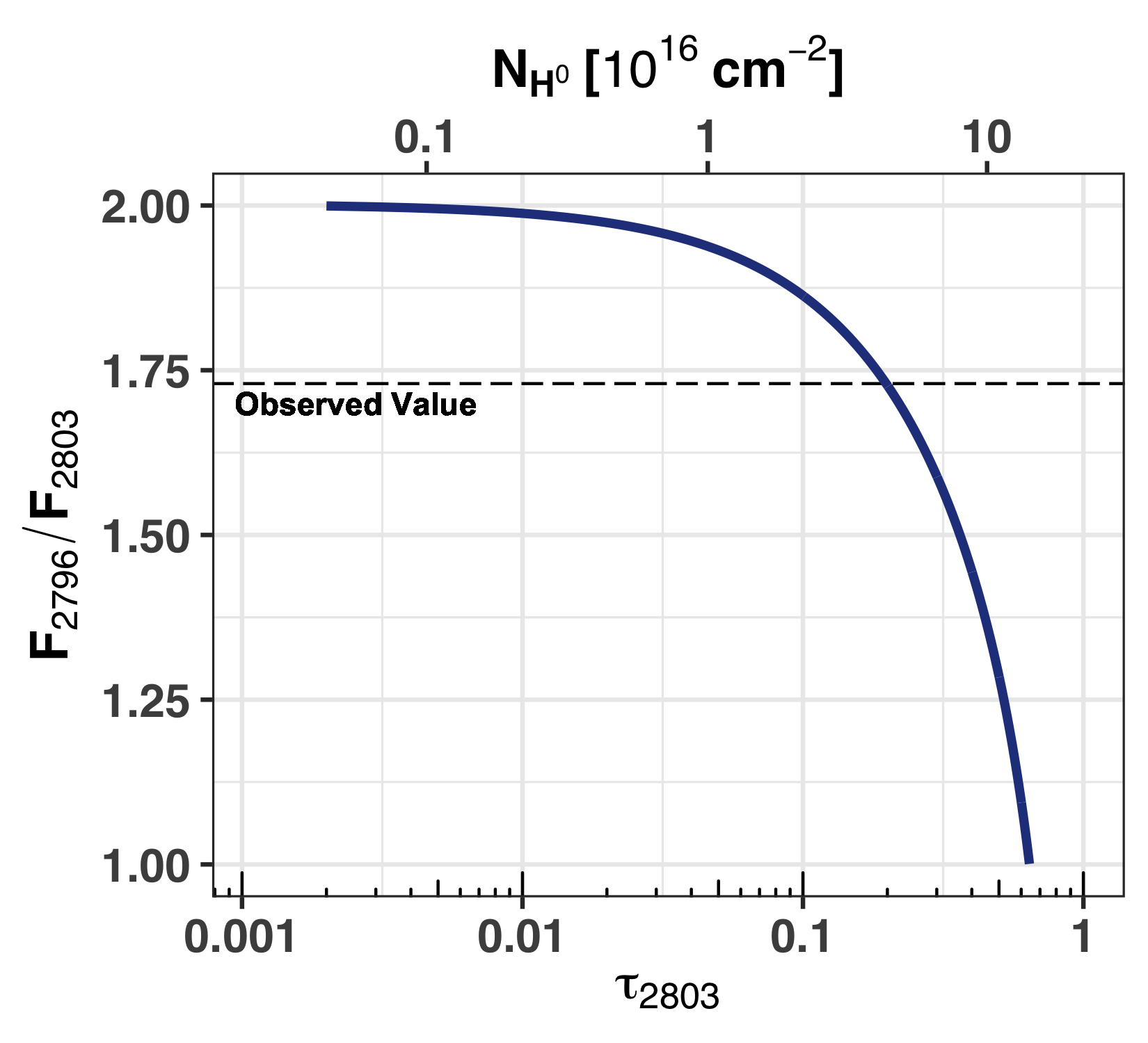
Figure 12: The change of the Mg ii doublet flux ratio, $R=F_{2796}/F_{2803}$, with the optical depth of the Mg ii 2803 Å line ($\tau_{2803}$) for a simple synthetic line profile that assumes that the nebular Mg ii emission is much brighter than the continuum emission (Section 6.2). The observed $R=1-2$ values from J1503 correspond to $\tau_{2803}$ values of 0.01–0.6, along the rapidly changing portion of the curve. The $R$ of optically thin Mg ii emission strongly varies with H⁰ column densities (upper x-axis, assuming the metallicity of J1503 and a typical dust depletion). Mg ii emission with $R>1$ corresponds to H⁰ column densities less than 10^17.2 cm^-2. Optically-thin Mg ii emission ($\tau_{2803}<1$) sensitively probes neutral gas column densities that allow ionizing photons to escape galaxies.

The first scenario envisions a uniform distribution of dustless, low column density Mg⁺ gas residing in the foreground along the line-of-sight to a background continuum plus Mg ii emission source (see Section 7 for the impact of dust). A small fraction of the incident light excites the Mg⁺ electrons into excited states. The Mg⁺ electrons then de-excite and emit Mg ii photons in random directions, predominately not along the line of sight. Since the Mg ii profile of J1503 indicates that the Mg⁺ is optically thin, these re-emitted Mg ii photons propagate through the Mg⁺ gas without being reabsorbed and are removed from along the line of sight to the observer. The transmitted Mg ii flux decreases, with the observed flux ($F_{\rm obs}$) given as

$$F_{\rm obs}=\left(F_{\rm int}+F_{\rm cont}\right)e^{-\tau}\approx F_{\rm int}e^{-\tau},$$ (6)

where $F_{\rm cont}$ is the background continuum and $F_{\rm int}$ is the background intrinsic Mg ii collisionally-excited nebular flux. Here we have approximated the intrinsic flux as being dominated by the Mg ii emission rather than the continuum flux (see Appendix C). $\tau$ is the optical depth of the transition integrated over the line profile, defined as

$$\tau=\frac{\pi e^{2}}{m_{\rm e}c^{2}}f\lambda N_{\rm Mg^{+}},$$ (7)

where $e$ and $m_{\rm e}$ are the electron charge and mass, $c$ is the speed of light, $\lambda$ is the restframe wavelength, and $f$ is oscillator strength of the transition. The $\tau$ ratio of the two Mg ii transitions is equal to the ratio of the $f$ values. $f_{2796}$ is twice that of the Mg ii 2803 Å transition, such that

$$\tau_{2796}=2\tau_{2803}.$$ (8)

Thus, if the intrinsic two-to-one Mg ii emission escapes through optically-thin Mg⁺ gas, $R$ is a function of $\tau_{2803}$ as

$$R=\frac{F_{\rm 2796,obs}}{F_{\rm 2803,obs}}=\frac{F_{\rm 2796,int}}{F_{\rm 2803,int}}e^{-\tau_{2796}+\tau_{2803}}=2e^{-\tau_{2803}}.$$ (9)

$R$ varies depending on $\tau_{2803}$ of the foreground Mg ii, and, through Equation 7, the Mg⁺ column density along the line of sight.

To illustrate how $R$ varies with $\tau_{2803}$ we created mock line profiles in three steps: (1) created a flat unity continuum level (consistent with the O-star dominated continuum spectrum of J1503), (2) added a Mg ii emission profile to the continuum with an $R_{\rm int}=2$, and (3) multiplied the resultant profiles by an absorption doublet profile with $\tau_{2803}$ (and $\tau_{2796}=2\tau_{2803}$). We assumed that both the emission and absorption profiles have the same velocities and widths. We then calculated $R$ the same way we did for the data. This process was repeated for a large range of $\tau_{2803}$ values to derive a distribution of $R$ values.

Figure 12 shows the change in $R$ with $\tau_{2803}$ for these mock spectra. As $\tau_{2803}\rightarrow 0$ the flux ratio tends to the intrinsic value of $R=2$ because there is no Mg⁺ gas along the line of sight to absorb Mg ii photons. As $\tau_{2803}$ increases, Mg⁺ removes a factor of $e^{\tau_{2803}}$ more flux from the 2796 Å line than from the 2803 Å line (Equation 9), resulting in a declining $R$ with increasing $\tau_{2803}$. Realistically observable $R$ values between $1-2$ probe $\tau_{2803}$ values between $0.6-0.01$, where extremely high-quality observations are required to estimate very low $\tau_{2803}$ values. This is the observed $R$ parameter space from J1503.

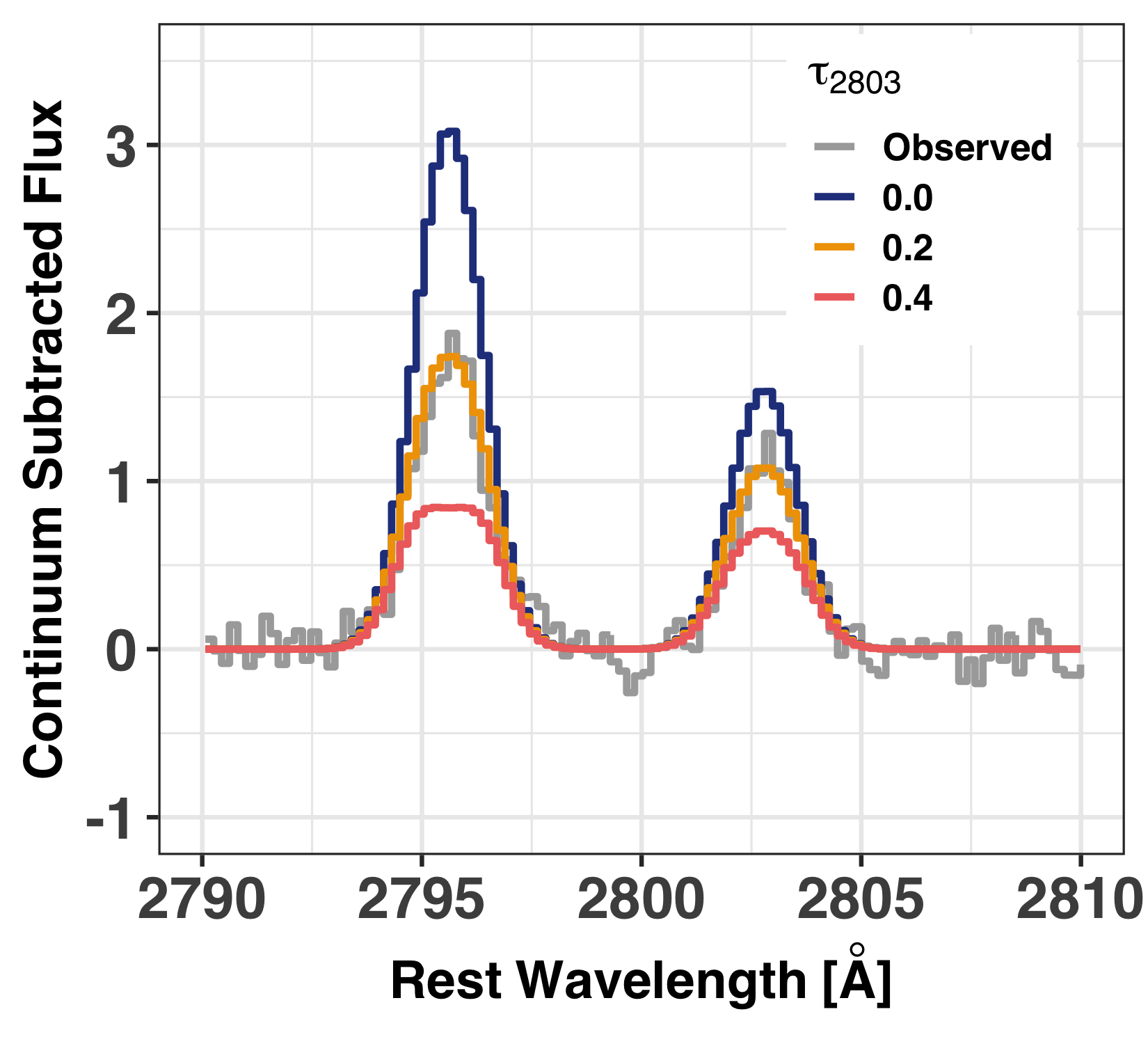
Figure 13: Simulated Mg ii doublet emission profiles for three different Mg ii 2803 Å optical depths ($\tau_{2803}$): 0 (blue), 0.2 (gold), and 0.4 (red). At $\tau_{2803}=0$, the line profiles have a flux ratio of 2. As $\tau_{2803}$ increases, the Mg ii 2796 Å line weakens by a factor of $e^{\tau_{2803}}$ more than the Mg ii 2803 Å line because the oscillator strength of the Mg ii 2796 Å is twice that of the Mg ii 2803 Å transition. The spatially integrated Mg ii profile from J1503 is included in gray and is consistent with the $\tau_{2803}=0.2$ model.

Mock spectra, with parameters tailored to the J1503 observations (Table 2), are shown in Figure 13. At $\tau_{2803}=0$ (dark blue line), the Mg ii profile is the intrinsic emission profile with a stronger Mg ii 2796 Å line than the Mg ii 2803 Å line and $R=2$. As $\tau_{2803}$ increases the 2796 Å profile decreases in strength until at $\tau_{2803}\sim 0.4-0.6$ the two Mg ii lines have similar strength (red line). In between $\tau_{2803}=0$ and $0.4$, the 2796 Å line is still stronger than the 2803 Å transition (gold line), but the relative strength of the two lines has noticeably decreased.

The observed spatially integrated Mg ii profile is included as a grey line in Figure 13. The mock profiles explain a few of the key observations. First, a small, optically-thin $\tau_{2803}$ of 0.2 (gold line) reproduces the spatially-integrated emission profile. The optically thin nature of Mg ii is consistent with the observations that the Mg ii emission is not spatially extended beyond the stellar or nebular emission (Figure 4 and Figure 6) and that the Mg ii line profiles are well-fit by single Gaussians centered at zero-velocity ( Figure 3). Second, the individual pixels (Figure 9) and the $R$ composites (Figure 11) show that decreasing the 2796 Å flux drives the $R$ from 2 to $\sim 1.3$, while the Mg ii 2803 Å line remains nearly constant. The mock spectra explain this shift because the 2796 Å transition has a larger oscillator strength and is reduced by a factor of $e^{\tau_{2803}}$ more than the 2803 Å transition.

Optical depth variations describe the foreground neutral gas properties in J1503 through which ionizing photons must pass through to escape the galaxy. First, Equation 9 directly infers $\tau_{2803}$ from the observed $R$ as

$$\tau_{2803}=-\ln\left(R/2\right).$$ (10)

Using the average value of $R=1.7$ from the spatially-integrated line profile, $\tau_{2803}=0.16$ over the entire galaxy of J1503 (Table 5). At these low optical depths, most of the $F_{\rm int}$ escapes the optically thin gas. Ignoring scattering because there are no observational signatures of either scattering or absorption, the amount of Mg ii emission that escapes J1503 can be inferred from Equation 6 as the escape fraction as

$$f_{\rm esc}\left({\rm\text{Mg\,{ii}}}\right)=\frac{F_{\rm obs}}{F_{\rm int}}=e^{-\tau}.$$ (11)

A $\tau_{2803}=0.16$ leads to $f_{\rm esc}\left(2803\right)=85\pm 7$% (Table 5).

Photoionization models can also predict $F_{\rm int}$ in Equation 11 by using multiple strong optical emission lines that are set by the ionization structure, metallicity, density, and ionizing continua of a hypothetical nebula (Erb et al., 2012; Guseva et al., 2013). Henry et al. (2018) used cloudy photoionization models (Ferland et al., 2017) to determine a relationship between the extinction-corrected [O iii] 5007 Å and [O ii] 3727 Å emission lines and $F_{\rm int}$(Mg ii) (their Eq. 2). Comparing $F_{\rm int}$ to the observed SDSS Mg ii 2803 Å line fluxes (Equation 11) suggests that J1503 transmits $95\pm 14$% of the Mg ii 2803 Å photons (Table 5). This is consistent with the $f_{\text{esc}}\left(\text{Mg\,{ii}}\right)$ estimated with $R$ above.

From Equation 7, the total Mg⁺ column density, $N_{{\rm Mg}^{+}}$, can be estimated in terms of $\tau_{2803}$ as

$$\begin{split}{N}_{{\rm Mg}^{+}}&=3.8\times 10^{14}~{}{\rm cm}^{-2}~{}\text{\AA}\frac{\tau_{2803}}{f\lambda}\\ &=4.4\times 10^{11}~{}{\rm cm}^{-2}~{}\tau_{2803},\end{split}$$ (12)

where we used the oscillator strength ($f=0.303$ for the 2803 Å transition) and the restframe wavelength (in Å). This is cast in terms of $R$ using Equation 10 as

$$N_{{\rm Mg}^{+}}=-4.4\times 10^{11}~{}{\rm cm}^{-2}~{}\ln\left(R/2\right).$$ (13)

Equation 13 implies that the spatially-integrated Mg⁺ column density in J1503 is $N_{{\rm Mg}^{+}}$ = $7\pm 3\times 10^{10}$ cm^-2.

The main goal of this paper is to relate the Mg ii emission to the LyC escape through the H⁰ column density. The Mg⁰ and Mg⁺ ionic phases overlap with H⁰ and their column densities can be converted into H⁰ column densities using the Mg/H abundance of the galaxy. There are two complications with this: (1) a rather uncertain fraction of Mg is depleted onto dust ($\delta_{\rm Mg}$) and (2) the Mg/H abundance must be determined. First, we assume that $\delta_{\rm Mg}=27$%, or that 27% of Mg is in the gas phase in the warm neutral medium (Jenkins, 2009). The Mg depletion factor has appreciable scatter, but a general trend is not observed with metallicity and the depletion only depends on the ionization for the most highly ionized galaxies (Guseva et al., 2019). Secondly, while the Mg/H abundance is challenging to observe, the O/H abundance is readily observable from multiple optical oxygen emission lines, some of which are temperature sensitive (e.g., [O iii] 4363 Å). Since both oxygen and magnesium are $\alpha$ elements that are primarily produced by core-collapse supernova (Johnson, 2019), the Mg/O value should not appreciably vary (except for dust depletion differences). Thus, we estimate the Mg/H abundance using the observed O/H abundance (see Table 1) and a solar O/Mg abundance of O/Mg $=12.3$ (Asplund et al., 2009). The H⁰ column density can then be approximated as:

$$\begin{split}{\rm N}_{{\rm H}^{0}}&=\frac{\rm H}{\rm O}\frac{\rm O}{\rm Mg}\frac{1}{\delta_{\rm Mg}}\left({\rm N}_{\rm Mg^{+}}+{\rm N}_{\rm Mg^{0}}\right)\approx 46\frac{\text{H}}{\text{O}}{\rm N}_{\rm Mg^{+}}\\ &\approx-2\times 10^{13}~{}{\rm cm}^{-2}~{}\frac{\rm H}{\rm O}\ln\left(R/2\right),\end{split}$$ (14)

where we neglected the contribution of Mg⁰ because the Mg i 2852 Å line is undetected in all our observations (individual spaxels or composites). Using the O/H of J1503, the assumed dust depletion, and Equation 13, the neutral hydrogen column density is expressed as

$$\begin{split}{\rm N}_{{\rm H}^{0}}&=5.1\times 10^{5}~{}{\rm cm}^{-2}~{}{\rm N}_{{\rm Mg}^{+}}\\ &=-2.2\times 10^{17}~{}{\rm cm}^{-2}\ln\left(R/2\right).\end{split}$$ (15)

Thus, the Mg ii doublet ratio and the gas-phase metallicity can infer the H⁰ column density. Equation 15 enables an unprecedented study of one of the chief sinks of ionizing photons within LyC emitters: the neutral hydrogen column density. The integrated H⁰ average column density over the entire galaxy of J1503 is $N_{\mathrm{H^{0}}}$ $=4\pm 1\times 10^{16}$ cm^-2.

Inverting Equation 15 provides guidelines for which $R$ values correspond to neutral gas that is optically thin to ionizing photons, assuming the nebular metallicity of J1503 and that dust destroys a negligible amount of ionizing photons (we refer to this as the relative escape fraction, $f_{\rm esc}^{\rm rel}$, see Section 7 for the importance of dust). Galaxies become optically thin to ionizing radiation at H⁰ column densities less than 10^17.2 cm^-2, which corresponds to an $R>0.97$ in J1503.

The metallicity crucially impacts the interpretation of whether Mg ii traces LyC escape. At a lower metallicity of 12+log(O/H) = 7.5, $R>1.6$ corresponds to a LyC emitter because there are fewer Mg atoms per hydrogen atom. Conversely, at solar metallicities (12+log(O/H) = 8.69; Asplund et al., 2009) galaxies with $R>0$ will be optically thin to ionizing radiation. Regardless of the gas-phase metallicity, $R\sim 2$ and Mg ii line profiles without signatures of scattering likely indicate H⁰ gas that is optically thin to ionizing radiation.

While this simple optical depth framework provides intuition for the propagation of ionizing photons through low column density neutral gas, some previous observations require further exploration. Namely, the Lyman Series of J1503 is strong (Gazagnes et al., 2018, 2020), implying a significant H⁰ column density. Strong saturated Lyman Series absorption is not just found in J1503, but other confirmed LyC emitting galaxies (Steidel et al., 2018).

6.3 Mg ii escape through a clumpy geometry

A possible solution is to have highly clumped neutral gas within the galaxy (Heckman et al., 2011; Zackrisson et al., 2013). Mg ii (and LyC) photons that encounter the dense clouds are absorbed and are not transmitted along the line of sight. Meanwhile, the channels between the clumps have zero column density and allow the photons to pass through these channels without being absorbed. Either large-scale gaseous instabilities (Kakiichi & Gronke, 2019) or massive star feedback (Jaskot et al., 2019) could inject the energy and momentum required to redistribute the optically-thick gas and create evacuated channels for the photons to pass through.

Envision that a fraction of the total area along the line of sight (called the covering fraction; $C_{f}$) is covered by high column density gas and 1-$C_{f}$ of the area is completely free of gas. Therefore, a fraction, 1-$C_{f}$, of the background radiation escapes the gas without being absorbed by Mg⁺, while the complement, $C_{f}$, of the light is absorbed by high column density Mg$+$ with an optical depth of $\tau\gg 1$. The radiative transfer equation (Equation 6; still neglecting dust) then takes the form of

$$F_{\rm obs}=F_{\rm int}\times\left[\left(1-C_{f}\right)+C_{f}e^{-\tau}\right]=F_{\rm int}\times\left(1-C_{f}\right),$$ (16)

where the simplistic geometry assumes that the gaseous regions are optically thick ($\tau\gg 1$). In this idealized scenario, all of the Mg ii photons that originate in optically thick regions are destroyed, either by dust or through scattering out of the line of sight. The observed Mg ii doublet flux ratio, which traces lines of sight through the empty channels, becomes simply

$$R=\frac{F_{\rm 2796,obs}}{F_{\rm 2803,obs}}=\frac{F_{\rm 2796,int}}{F_{\rm 2803,int}}=2,$$ (17)

because both transitions have the same $C_{f}$ at $\tau\gg 1$. The extremely clumpy scenario predicts that $R$ does not vary from the intrinsic $R$. Rather, any Mg ii emission that escapes the neutral gas has the flux ratio equal to the intrinsic ratio. However, the observations of J1503 demonstrate a variation of $R$ values. Thus, neither of these overly-simplified physical scenarios match all of the observations.

6.4 Mg ii escapes through low column density channels surrounded by high column density regions

Both of the proposed scenarios above reproduce portions of the observations, but neither satisfies all the constraints. A slight modification of the extremely clumpy scenario is that the channels that photons pass through have a low column density medium, with $\tau_{\rm chan}$, while the optically-thick regions, with $\tau_{\rm thick}$, absorb all of the photons incident upon them (Gazagnes et al., 2020). This modifies the radiative transfer equation in Equation 16 to become

$$F_{\rm obs}=F_{\rm int}\times\left[\left(1-C_{f}\right)e^{-\tau_{\rm chan}}+C_{f}e^{-\tau_{\rm thick}}\right].$$ (18)

If $\tau_{\rm thick}\gg 1$, the Mg ii doublet flux ratio becomes

$$\frac{F_{\rm 2796,obs}}{F_{\rm 2803,obs}}=\frac{F_{\rm 2796,int}}{F_{\rm 2803,int}}\frac{\left(1-C_{f}\right)e^{-2\tau_{\rm 2803,chan}}}{\left(1-C_{f}\right)e^{-\tau_{\rm 2803,chan}}}$$ (19)

and the observed $R$ becomes

$$R=2e^{-\tau_{\rm 2803,chan}}.$$ (20)

This equation is nearly identical to the $R$-relation found in the optically thin scenario (Equation 9) but with the important physical clarification that the Mg ii flux ratio is entirely determined by the optical depth of the low column density channels. All of the derivations in Section 6.2 that relate Mg ii emission to the H⁰ properties hold, but have the crucial physical distinction that they only correspond to the gas within the low column density channels.

Is this scenario of low column density gas in between higher column density clouds consistent with the Lyman Series observations? Gazagnes et al. (2018) and Gazagnes et al. (2020) used the observed Ly$\beta$, Ly$\gamma$, Ly$\delta$, and Ly5 absorption lines of J1503 to determine that the Lyman series is saturated, but the fitted Lyman Series covering fraction is $0.72\pm 0.06$. Ly$\beta$ is the strongest transition fit by Gazagnes et al. (2020), and Ly$\beta$ saturates at $N_{\mathrm{H^{0}}}$ $\gtrsim 8\times 10^{15}$ cm^-2. In other words, the Gazagnes et al. (2020) observations indicate that 72% of the area of the stellar continuum is covered by neutral gas with $N_{\mathrm{H^{0}}}$ $\gtrsim 8\times 10^{15}$ cm^-2. Using Equation 15, we find that 67% of the stellar continuum in J1503 is covered by Mg ii gas with $R<1.928$ (the $R$ that corresponds to $8\times 10^{15}$ cm^-2), similar to the observed Lyman Series covering fraction. This suggests that the Mg ii emission can serve as a proxy of the neutral gas properties.

Likewise, the covering fraction of optically thick Mg⁺ gas can be estimated by combining Equation 11 and Equation 18 as

$$\text{$f_{\text{esc}}\left(\text{Mg\,{ii}}\right)$}=\left(1-C_{f}(\text{\text{Mg\,{ii}}})\right)e^{-\tau_{\rm chan}}.$$ (21)

If $f_{\text{esc}}\left(\text{Mg\,{ii}}\right)$ is measured using photoionization models (such as from Henry et al., 2018) and $\tau_{\rm chan}$ is estimated using $R$ (which is independent of $C_{f}$; see Equation 20), the Mg ii covering fraction can be approximated as

$$C_{f}(\text{\text{Mg\,{ii}})}=1-\text{$f_{\text{esc}}\left(\text{Mg\,{ii}}\right)$}e^{\tau_{\rm chan}}.$$ (22)

Using the spatially-integrated values (Table 5), this leads to a $C_{f}(\text{\text{Mg\,{ii}})}=-0.11\pm 0.05$. At a 2$\sigma$ significance level, this $C_{f}(\text{\text{Mg\,{ii}})}$ is a non-physical $C_{f}$ that is less than zero. This implies that either $f_{\text{esc}}\left(\text{Mg\,{ii}}\right)$ is over-estimated or $\tau_{\rm chan}$ is slightly under-estimated. The mis-estimate could possibly arise from either the effects of absorption subsequently followed by re-emission (or scattering, which is not accounted for here) or issues with the photoionization models. Regardless, the low inferred $C_{f}$ agrees with the fact that we do not observe any spaxels with $R<0.7$, which corresponds to $\tau_{\rm chan}=1$, and that $C_{f}(\text{\text{Mg\,{ii}})}\approx 0$. Thus, a small $C_{f}(\text{\text{Mg\,{ii}})}$ can be inferred from both the spatially resolved and spatially-unresolved observations.

Meanwhile, $C_{f}(\text{H}^{0})$ is required to estimate the LyC escape fraction. The $C_{f}$ inferred from the Lyman Series or the metal absorption lines does not properly quantify the covering of H⁰ related to LyC escape because these transitions become optically thick at different column densities than the LyC. Equation 18 defines $C_{f}$ as the fraction of the total sight lines with $\tau\gg 1$. For LyC emission, this can be recast in terms of the fraction of sightlines that intersect H⁰ gas with $N_{\mathrm{H^{0}}}$ $>10^{17.2}$ cm^-2. Figure 10 indicates that no observed spaxel has Mg ii emission that suggests $\tau_{\text{\rm{H}${}^{0}$}}\gg 1$ and only 1.6% of the spaxels have $R<0.97$ and $\tau_{\text{\rm{H}${}^{0}$}}\gtrsim 1$. This implies that, at least for J1503, $C_{f}(\text{\rm{H}${}^{0}$})\approx 0$ for gas that is optically thick to the LyC.

The neutral gas covering fraction can be approximated using $\tau_{\rm chan}$ and $f_{\text{esc}}\left(\text{Mg\,{ii}}\right)$, if the abundance is such that Mg ii becomes optically thick at the same $N_{\mathrm{H^{0}}}$ as the Lyman Break (10^17.2 cm^-2). For J1503, $R>1.0$ corresponds to optically thin neutral hydrogen and $R>0.7$ corresponds to optically thin Mg ii. Thus, $C_{f}(\text{\text{Mg\,{ii}})}$ provides an upper limit for $C_{f}(\text{\rm{H}${}^{0}$})$ in J1503.

Meanwhile, at a slightly higher 12+log(O/H) = 8.1, the Mg ii covering fraction exactly equals the H⁰ covering fraction. If the Mg ii covering fraction differs from the H⁰ covering fraction, $C_{f}(\text{\text{Mg\,{ii}})}$ can only provide limits for $C_{f}(\text{\rm{H}${}^{0}$})$. If $C_{f}(\text{\text{Mg\,{ii}})}$ is large, then the neutral gas covering fraction must be accounted for when estimating the $f_{\text{esc}}$$\left({\rm LyC}\right)$. Conversely, if $C_{f}(\text{\text{Mg\,{ii}})}$ is small, then the covering fraction can be approximated as zero.

This is not to say that LyC passes through the low column density channels unabsorbed, rather the LyC optical depth is less than 1. The strong correlations between the $C_{f}$ of the Lyman Series and $f_{\text{esc}}$$\left({\rm LyC}\right)$ and the Ly$\alpha$ properties (Steidel et al., 2018; Gazagnes et al., 2020) could arise because the $N_{\mathrm{H^{0}}}$ distribution within a galaxy is rather broad (Figure 10). The LyC escapes through the lowest column density gas, and the fraction of H⁰ that is optically thin to LyC depends on the median and shape of the $N_{\mathrm{H^{0}}}$ distribution. Thus, if $N_{\mathrm{H^{0}}}$ is low on average, fewer total sight lines would have optically thick Lyman Series absorption lines and the $C_{f}$ will be lower.

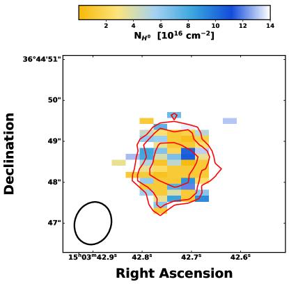
Figure 14: The spatial distribution of the H⁰ column density in J1503 calculated using the Mg ii doublet flux ratio and assuming a constant nebular metallicity and dust depletion (Equation 15). The contours show the 2, 5, and 10$\epsilon$ contours of the integrated Mg ii emission. Gold regions correspond to low H⁰ column density and are patchy over the face of the galaxy. The low column density regions are likely the channels through which the ionizing photons escape J1503.

Thus, the Mg ii observations suggest that J1503 emits ionizing photons due to a combination of the two proposed scenarios: the H⁰ column density is low (a spatially averaged value of $4\times 10^{16}$ cm^-2), but the column density also has a broad spatial distribution. Figure 14 shows the spatial map of $N_{\mathrm{H^{0}}}$ and depicts a factor of more than 10 variation in the H⁰ column density. This clumpy H⁰ distribution suggests that ionizing photons escape through the regions of relatively low H⁰ column density (the light blue regions in Figure 14) with sizes smaller than, or on the order of, the 5 kpc spatial resolution of the observations.

7 An ideal Lyman Continuum tracer

A chief goal of this study is to provide an indirect method for future observations to infer the absolute escape fraction of ionizing photons, $f_{\text{esc}}$$\left({\rm LyC}\right)$, from galaxies within the Epoch of Reionization. Above we proposed the combination of the Mg ii doublet and nebular metallicities as an ideal tracer of the H⁰ column density. The combination of $N_{\mathrm{H^{0}}}$ and dust attenuation then provides an estimate of the absolute LyC escape fraction. In this section we walk through the process of inferring $f_{\text{esc}}$$\left({\rm LyC}\right)$ from the Mg ii observations of J1503 (Section 7.1), and how $f_{\text{esc}}$$\left({\rm LyC}\right)$ spatially varies (Section 7.2). We then calculate $f_{\text{esc}}$$\left({\rm LyC}\right)$ using literature Mg ii observations of 6 other known LyC emitters (Section 7.3). In Section 7.4, we comment on the possibility of observing Mg ii with JWST and ELTs to constrain the sources of cosmic reionization.

7.1 The LyC escape fraction of J1503

Ionizing radiation is absorbed by two main sinks: H⁰ gas and dust. Breaking up the contributions of the two simplifies the determination of the absolute escape fraction, or $f_{\text{esc}}$$\left({\rm LyC}\right)$. The fraction of ionizing photons that pass through a dustless neutral medium, sometimes referred to as the relative escape fraction, is

$$\begin{split}f_{\rm esc}^{\rm rel}&=e^{-N_{{\rm\textsc{H}}^{0}}\sigma_{\rm phot}}\\ &\approx e^{2.2\times 10^{17}~{}{\rm cm}^{-2}\sigma_{\rm phot}\ln{R/2}},\end{split}$$ (23)

where $\sigma_{\rm phot}=6.3\times 10^{-18}$ cm² is the photoionization cross-section of H⁰ at 912 Å. Using $N_{\mathrm{H^{0}}}$ $=3.6\times 10^{16}$ cm^-2, the average column density inferred from the spatially-integrated Mg ii emission from Equation 15, 80% of the intrinsic ionizing photons pass through the dustless neutral gas in J1503. For the metallicity of J1503, $f_{\rm esc}^{\rm rel}$ and $f_{\text{esc}}\left(2803\right)$ are statistically consistent with each other (Table 5). However, this will not always be true and will depend on the metallicity of the gas.

Dust is the second sink of ionizing photons. The fraction of ionizing photons at 912 Å that pass through a dusty medium without being absorbed is given as

$$f_{\rm esc}^{\rm Dust}=10^{-0.4{\rm E(B-V)k(912)}}.$$ (24)

Gazagnes et al. (2020) used the Reddy et al. (2016) attenuation law, with k(912) $=$ 12.87, to fit theoretical stellar continuum models to the observed FUV stellar continuum features of J1503. The FUV stellar continuum is best-fit with E(B-V) = 0.22 mag. This can be compared to the E(B-V) $=0.09$ that Izotov et al. (2016a) calculated for J1503 using the Balmer emission lines. However, the Izotov et al. (2016a) value was determined using the Cardelli et al. (1989) attenuation law with $R_{V}=2.3$, whereas we used the Reddy et al. (2016) law. If we calculate E(B-V) using the observed H$\alpha$/H$\beta$, H$\gamma$/H$\beta$ and H$\delta$/H$\beta$ flux ratios from Izotov et al. (2016a) and the Reddy et al. (2016) attenuation law, we estimate E(B-V)$=0.14,0.21,0.23$ mag, respectively. Thus, the stellar and nebular attenuations are similar when similar attenuation laws are used. This relatively large inferred E(B-V) means that dust removes a large fraction of the ionizing photons; only 7% of the ionizing photons escape the galaxy without being absorbed by dust ($f_{\rm esc}^{\rm Dust}$). As stressed by Chisholm et al. (2018), dust is the major sink of ionizing photons in J1503.

The total, or absolute, $f_{\text{esc}}$$\left({\rm LyC}\right)$ is equal to the product of the relative escape fraction and the fraction unabsorbed by dust such that

$$f_{\rm esc}\left({\rm LyC}\right)=e^{-N_{{\rm\textsc{H}}^{0}}\sigma_{\rm ph}}\times 10^{-0.4\text{E(B-V) k(912)}}.$$ (25)

This leads to an absolute $f_{\text{esc}}$$\left({\rm LyC}\right)$ $=5.9\pm 0.4$% from the spatially-integrated observations. This is consistent with the $f_{\text{esc}}$$\left({\rm LyC}\right)$ directly observed from the LyC of $5.8\pm 0.6$% (Izotov et al., 2016a). Thus, the escape fraction of ionizing photons from J1503 can be recovered using the Mg ii doublet flux ratio and the dust attenuation.

Note that the covering fraction does not appear in the estimation of $f_{\text{esc}}$$\left({\rm LyC}\right)$, even though we assumed a highly clumpy, non-uniform geometry. As discussed in Section 6.4, this is because hardly any of the observed spaxels have Mg ii emission properties that indicate optically thick H⁰. This effectively means that $C_{f}(\text{\rm{H}${}^{0}$})~{}=~{}0$. The Mg ii covering fraction (Equation 22) from spatially unresolved observations can be used as a guide for whether the neutral covering fraction must be included, but only if the abundance is close to 12+log(O/H) = 8.1, Mg⁺ is the dominant neutral ionization state, and the dust depletion is similar to our assumptions (see Section 6.4).

Further, the Mg ii emission profile itself indicates that the individual spaxels have near zero covering fractions of optically thick gas because there are no strong indications of absorption or scattering, with only minor, <3$\sigma$ significant, deviations from the single Gaussian fit (Figure 3, Figure 9, and Figure 11). If there was both optically thin and optically thick gas along the line of sight, a complex profile, with absorption and emission, would be observed. Such complex Mg ii profiles have been observed in galaxy spectra at moderate redshifts (Erb et al., 2012; Guseva et al., 2013; Martin et al., 2013; Rubin et al., 2014; Finley et al., 2017; Feltre et al., 2018; Burchett et al., 2020), but are not observed from J1503. Further, at larger Mg ii optical depths, radiative transfer effects will impact the resultant Mg ii emission profiles: shifting the velocities of emission lines away from zero velocity, broadening the lines, decreasing $f_{\text{esc}}\left(\text{Mg\,{ii}}\right)$, and leading to non-Gaussian profiles (Henry et al., 2018). Any of these more complex profiles would strongly suggest that either $\tau_{2803}$ or $C_{f}(\text{Mg\,{ii}})$ are large, indicating that $R$ cannot be used to robustly determine $\tau_{2803}$ and $f_{\text{esc}}$$\left({\rm LyC}\right)$.

7.2 The LyC escape fraction in different regions of J1503

In Section 4 we found that the Mg ii doublet flux ratio, $R$, varies spatially in J1503. Combined with the hypothesis that ionizing photons escape through low column density channels in a denser medium (Section 6.4), this spatial $R$ variation suggests that $f_{\rm esc}^{\rm rel}$ varies from location-to-location within J1503. Here we first explore the spatial variation of the higher S/N composites and then the individual spaxel-by-spaxel variations.

The $N_{\mathrm{H^{0}}}$ values in the High and Low $R$ composites are $4\pm 8\times 10^{15}$ and $7\pm 1\times 10^{16}$ cm^-2 (Figure 11 and Table 4). This is a factor of 18 difference (with a 4$\sigma$ separation) in H⁰ column density between the two composites that translates to relative escape fractions of 97 and 63%, respectively, if we assume that there is a constant metallicity and dust depletion. Similarly, the four spatially distinct integrated regions (Table 3) have relative escape fractions between $>88$ and 67%. While this difference in the relative escape fraction is significant, it does not fully explain total the spatial variation of the absolute $f_{\text{esc}}$$\left({\rm LyC}\right)$.

Dust attenuation can also strongly vary spatially, especially if the dust column density is related to the total neutral column density through a dust-to-gas ratio. In Section 7.1, we used stellar fits to the FUV stellar continuum to determine the dust reddening for spatially integrated FUV observations. Another common way to measure the dust attenuation is the ratio of recombination emission lines that have intrinsic intensity ratios set by atomic physics. The Balmer emission lines are the most typical way to infer the reddening from emission lines, but our narrow wavelength regime does not contain Balmer lines. However, the He i 3188 Å and He i 2945 Å lines are both He i recombination lines whose intrinsic ratios are set by atomic physics, if the electron temperature and density are constrained (Table 1). The He i lines are not ideal to trace the attenuation because their intrinsic strength varies more with temperature and density than Balmer lines, and future observations will explore this limitation. The intrinsic He i 3188 Å to He i 2945 Å flux ratio, for the observed temperatures and densities (Benjamin et al., 1999), is

$$\frac{F_{\rm 3188,int}}{F_{\rm 2945,int}}=2.1.$$ (26)

The He i 2945 Å emission in the High and Low $R$ composites are weak, but the He i flux ratio is different at the $1.5\sigma$ significance levels in the two stacks (Table 4). The flux ratio for the High $R$ stack is nearly 2.1, while the Low $R$ stack has a larger He i flux ratio. This rough comparison implies that the High $R$ stack has less dust attentuation than the Low $R$ stack.

We estimate E(B-V) values for both composites by assuming the Reddy et al. (2016) reddening law and comparing the observed and intrinsic $F_{3188}/{F_{2945}}$ (Table 5). This suggests that the Low $R$ composite has higher $N_{\mathrm{H^{0}}}$ regions and more dust attenuation. When we determine the absolute escape fraction of the Low $R$ regions with these inferred dust attenuations, we find that it is zero. The combination of the higher dust attenuation and H⁰ column density in these more optically thick regions means that all of the ionizing photons are absorbed. Meanwhile, the High $R$ composite has both lower dust attenuation and lower $N_{\mathrm{H^{0}}}$, such that 19% of the ionizing photons escape the galaxy. This suggests that all of the ionizing photons that escape J1503 come from the High $R$ regions.

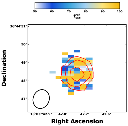
Figure 15: The spatial variation of the relative escape fraction of ionizing photons, or the escape fraction without accounting for dust. The red contours are the 2, 5, and 10$\epsilon$ stellar continuum flux. There is a factor of two difference between regions of high (gold) and low (blue) relative escape fractions. The LyC escape fraction varies spatially across the galaxy. The black circle gives the observed seeing.

Another way to demonstrate the spatial variation is to consider $f_{\rm esc}^{\rm rel}$. Figure 15 shows that $f_{\rm esc}^{\rm rel}$ varies spatially by a factor of two, where gold regions have relative escape fraction near 100% and blue regions are as low as a 44%. The stellar continuum (red contours in Figure 15) weighted relative escape fraction is 83%, consistent with the relative escape fraction of 80% calculated from the spatially-integrated Mg ii line profiles (Section 7.1). Thus, the spatially resolved escape fraction for J1503 is similar to the spatially-integrated value.

The Mg ii observations suggest that ionizing photons escape from J1503 through regions of low H⁰ column density that are embedded within regions of slightly higher, but still relatively low, H⁰ column density. As stressed in Section 6.4, the escape fraction determined by the Mg ii emission lines is only through these low column density channels. The variations in the $N_{\mathrm{H^{0}}}$ and dust attenuation in these low column density channels imprint spatial variations on the escape fraction of ionizing photons (Figure 15). This introduces a crucial orientation effect for the interpretation of the observed escape fractions: whether the observer is along a line of sight to low column density dust-free channel or high column density dusty region determines whether LyC is observed (Zackrisson et al., 2013; Micheva et al., 2018, 2019; Fletcher et al., 2019).

7.3 Mg ii reproduces the LyC escape fraction

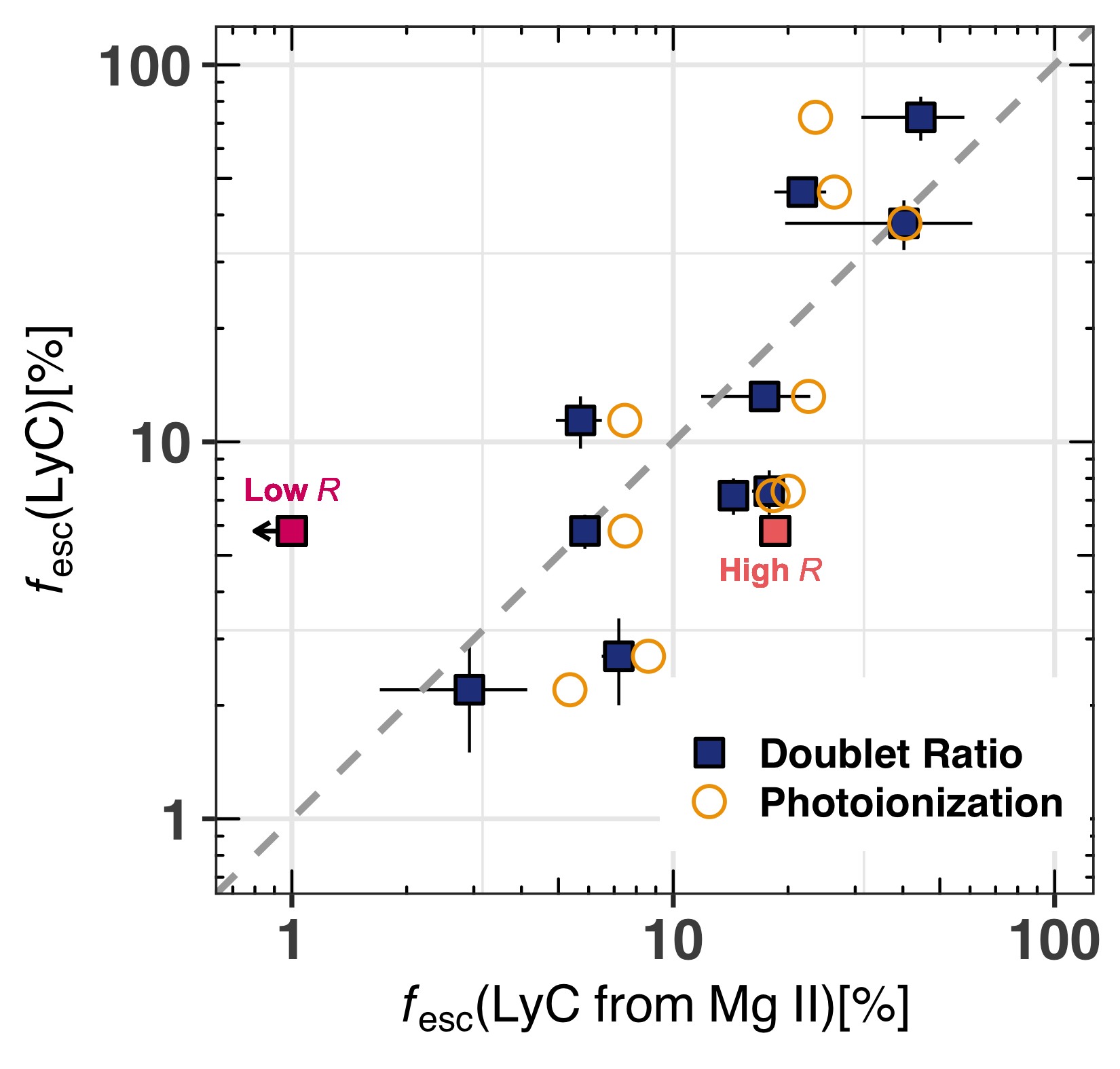
Figure 16: The directly observed absolute LyC escape fraction ($f_{\text{esc}}$$\left({\rm LyC}\right)$) versus the escape fraction predicted using the Mg ii emission and the FUV stellar continuum attenuation (see Section 7.1) for 10 confirmed LyC emitters from the literature (listed in Table 6; Izotov et al., 2016a, b; Izotov et al., 2018a; Izotov et al., 2018b; Guseva et al., 2020) . We predicted the escape fraction in two ways: using the Mg ii doublet flux ratio (blue squares) and the photoionization models from Henry et al. (2018) (gold circles). The predicted LyC escape fractions from both methods accurately reproduce $f_{\text{esc}}$$\left({\rm LyC}\right)$ (see the gray dashed one-to-one line). This suggests that the Mg ii emission, nebular metallicity, and dust continuum attenuation can be used to predict $f_{\text{esc}}$$\left({\rm LyC}\right)$ of high-redshift galaxies. The red points are the LyC escape fraction observed from composites of spaxels with Low and High $R$, demonstrating that all of the ionizing photons in J1503 escape through regions with High $R$. Regions with Low $R$ have $f_{\text{esc}}$$\left({\rm LyC}\right)$ $\sim$ 0.

Table 6: Properties of LyC emitting galaxies from Izotov et al. (2016a), Izotov et al. (2016b), Izotov et al. (2018a), and Izotov et al. (2018b) used to infer the LyC escape fractions using the Mg ii emission doublet. The first column gives the galaxy’s name. The second column gives the nebular oxygen abundance. The third column gives the Mg ii doublet flux ratio ($R$) from the SDSS (Izotov et al., 2016b, a; Izotov et al., 2018a; Izotov et al., 2018b), from Guseva et al. (2020) (for J1154+2443, J1011+1947, J1442-0209, J0925+1403, and J0901+2119), or the KCWI observations presented here (for J1503+3644). The forth column gives the attenuation of the FUV stellar continuum (Gazagnes et al., 2020). The fifth column gives the [O iii]/[O ii] flux ratio (O₃₂) that has been corrected for internal extinction using the value from the Balmer ratio (Izotov et al., 2016a, b; Izotov et al., 2018a; Izotov et al., 2018b; Guseva et al., 2020). The sixth column gives the Mg ii 2803 Å to [O iii] 5007 Å flux ratio corrected for internal attenuation with the nebular Balmer-line extinction correction. Columns 7-9 are the directly observed absolute LyC escape fraction ($f_{\text{esc}}$$\left({\rm LyC}\right)$; Izotov et al., 2016a, b; Izotov et al., 2018a; Izotov et al., 2018b), the LyC escape fraction inferred from the Mg ii doublet flux ratio ($f_{\rm esc}$(LyC from Mg ii); Equation 25), and the LyC escape fraction inferred using the photoionization models of Henry et al. (2018) (using columns 5 and 6 and their Eq. 2; $f_{\rm esc}(\rm phot)$). Both $f_{\rm esc}$(LyC from Mg ii) and $f_{\rm esc}(\rm phot)$ have been corrected with the same FUV dust attenuation from Gazagnes et al. (2020).

Name	12+log(O/H)	$F_{2796}/F_{2803}$	E(B-V)	O32	log(Mg/[O iii])	$f_{\text{esc}}$$\left({\rm LyC}\right)$	$f_{\rm esc}\left({\rm LyC~{}from~{}\text{Mg\,{ii}}}\right)$	$f_{\rm esc}\left({\rm phot}\right)$
(1)	(2)	(3)	(4)	(5)	(6)	(7)	(8)	(9)
J1243+4646	7.89	$2.5\pm 0.8$	0.10	13.5	-1.44	73	$45\pm 13$	24
J1154+2443	7.75	$1.9\pm 0.3$	0.12	11.5	-1.93	46	$14\pm 3.5$	26
J1256+4504	7.87	$2.0\pm 1.0$	0.08	16.3	-1.92	38	$40\pm 21$	40
J1152+3400	8.00	$1.9\pm 0.6$	0.14	5.4	-1.91	13	$17\pm 5.5$	23
J1011+1947	7.97	$1.8\pm 0.2$	0.23	27.1	-2.39	11	$5.7\pm 0.8$	7.4
J1442-0209	7.99	$1.9\pm 0.2$	0.14	6.7	-1.70	7.4	$24\pm 17$	20
J0925+1403	8.12	$2.0\pm 0.2$	0.16	5.0	-1.92	7.2	$14\pm 1.0$	18
J1503+3644	7.95	$1.7\pm 0.1$	0.22	4.9	-1.52	5.8	$5.9\pm 0.4$	7.5
J0901+2119	8.05	$2.0\pm 0.2$	0.22	8.0	-1.96	2.7	$7.2\pm 0.7$	7.4
J1248+4259	7.64	$1.7\pm 0.7$	0.25	11.8	-1.95	2.2	$2.9\pm 1.2$	5.4

J1503 is just a single example of a LyC emitting galaxy with Mg ii emission. Of the 11 galaxies with confirmed LyC emission in the Izotov et al. (2016a), Izotov et al. (2016b), Izotov et al. (2018a), and Izotov et al. (2018b) samples, five are at redshifts $z>0.34$ where Mg ii is redshifted into the SDSS DR15 wavelength regime. For four of the five SDSS spectra, we take the literature extinction-corrected $R$ and metallicity measurements, while we downloaded the SDSS data for J1243+4646 and measured the extinction-corrected Mg ii values ourselves (Table 6). An additional five have been observed with xshooter on the VLT and have strong Mg ii detections (Guseva et al., 2020). Thus, we have a sample of 10 galaxies with both Mg ii emission and LyC detections.

We use the HST/COS FUV stellar continuum observations to determine the dust attenuation following the methods Chisholm et al. (2019) and published in Gazagnes et al. (2020). These measurements estimate the absolute LyC escape fraction using the Mg ii doublet and dust attenuation the same way we did in Section 7.1. The inferred $f_{\text{esc}}$$\left({\rm LyC}\right)$ from the Mg ii, the blue squares in Figure 16, strongly follow the $f_{\text{esc}}$$\left({\rm LyC}\right)$ directly observed from the LyC with a 3$\sigma$ statistical significance (p-value < 0.001; Pearson’s correlation coefficient of 0.88).

Similarly, photoionization models from Henry et al. (2018) and the FUV attenuation can predict $f_{\text{esc}}$$\left({\rm LyC}\right)$ in a manner that is complementary to $R$ (gold circles). We use the dust corrected [O iii] 5007 Å and [O ii] 3727 Å values from Izotov et al. (2016a), Izotov et al. (2016b), Izotov et al. (2018a), Izotov et al. (2018b), and Guseva et al. (2020) to estimate the intrinsic Mg ii 2803 Å emission using the photoionization models of Henry et al. (2018) (their Eq. 2). We then compare the observed Mg ii emission fluxes to the expected intrinsic Mg ii emission to determine $f_{\text{esc}}\left(2803\right)$ (Equation 11). We then dust correct the $f_{\text{esc}}\left(2803\right)$ ratios in the same exact way as we did when calculating $f_{\text{esc}}$$\left({\rm LyC}\right)$ using $R$. The only difference between the blue squares and gold circles in Figure 16 is the determination of $F_{\rm int}$ (either with $R$ or photoionization models). Comparing the two methods indicates that both reasonably reproduce the absolute LyC escape fraction. While a small sample-size, the sample of Mg ii and LyC emitters spans the full observed range of $f_{\text{esc}}$$\left({\rm LyC}\right)$ from 2-73%, suggesting that the Mg ii doublet and the dust attenuation can infer the LyC escape fraction over a wide $f_{\text{esc}}$$\left({\rm LyC}\right)$.

7.4 The Mg ii Doublet May Determine the Escape Fraction of EoR Galaxies

J1503 is a local LyC emitter with a $z\sim 0.3$. The Mg ii observations presented here provide a template to constrain the escape fraction of ionizing photons from galaxies within the Epoch of Reionization. In the next 5–10 years the advent of the James Webb Space Telescope (JWST) and 20–40 m class Extremely Large Telescopes (ELTs) will provide the necessary collecting area and reduced FIR backgrounds to definitively measure the Mg ii doublet ratio, the dust attenuation, and the nebular metallicities of these distant galaxies. The methods presented in Section 7.3 can then determine $f_{\text{esc}}$$\left({\rm LyC}\right)$ of galaxies within the Epoch of Reionization. These inferences will be the first indirect constraints on the LyC escape fraction of star-forming galaxies during the Epoch of Reionization, testing crucial galaxy and AGN formation and evolution models.

Is it feasible to empirically infer the escape fractions of ionizing photons using Mg ii and the next generation of telescopes? Recent observational campaigns with HST have found galaxies within the EoR with F160W (mean wavelength of 1.5 $\mu$m) magnitudes near 25 mag (Livermore et al., 2017; Oesch et al., 2018). When the Spitzer imaging is included, the Spectral Energy Distributions require mean [O iii]+H$\beta$ equivalent widths near 650 Å and extreme values up to 2600 Å (Labbé et al., 2013; Smit et al., 2015; De Barros et al., 2019). Assuming that the stellar continuum is flat in $F_{\nu}$ and that the H$\beta$ equivalent width is 0.2 times the combined H$\beta$+[O iii] equivalent width (for a mean H$\beta$ equivalent of 215Å, consistent with J1503), the average (extreme) of these $z\sim 7$ galaxies would have observed H$\beta$ fluxes of $2\times 10^{-18}$ ($8\times 10^{-18}$) erg s^-1 cm^-2. With $F$(Mg ii 2796) $=1/3F$(H$\beta$) from J1503, we expect these bright $z\sim 7$ galaxies to have $F$(Mg ii 2796) = $6\times 10^{-19}$ ($3\times 10^{-18}$) erg s^-1 cm^-2. Note that Guseva et al. (2013) find galaxies in the local Universe with Mg ii/H$\beta$ flux ratios as high as 0.6. J1503 could be a conservative estimate.

The JWST NIRSpec Exposure Time Calculator predicts that a 10 hr observation would detect Mg ii 2796 Å with a S/N of 5 (17) per pixel with a resolving power of $\sim 2000$, or $\sim 150$ km s^-1, at 2.2 $\mu$m using the G235H grating. These spectral resolutions are required to resolve the Mg ii emission properties and rule out possible impacts of absorption and scattering. Combining the Mg ii observations with a measured dust attenuation and metallicity will determine the absolute escape fraction of galaxies within the Epoch of Reionzation. A 10 hr integration is large, but the Multi-Object Spectroscopy capabilities of JWST enables for $f_{\text{esc}}$$\left({\rm LyC}\right)$ to be simultaneously inferred for multiple $z\sim 6-10$ galaxies. Similarly, future ELTs will have extreme collecting areas coupled with the next generation of Adaptive Optics. This will enable Mg ii observations in the K-band out to $z\sim 7.5$. From the ground, these observations will determine the $R$ values for galaxies within the Epoch of Reionization which can be combined with restframe FUV continuum observations in the observed Y and H-bands to determine the escape fractions of galaxies within the Epoch of Reionization.

8 Summary

Here we presented Keck Cosmic Web Imager (KCWI) spatially-resolved spectroscopic observations of the Mg ii 2796, 2803 Å doublet from J1503+3644. J1503+3644 is a $z\sim 0.36$ Lyman Continuum emitter with a spatially averaged 6% escape fraction of ionizing photons. Mg ii is a resonant transition with an ionization potential of 15 eV that overlaps in ionization state with H⁰. Thus, Mg ii provides an opportunity to determine the properties of the neutral gas that ionizing photons must propagate through to escape the galaxy. These observations are a test-case for indirectly determining the escape fraction of ionizing photons from galaxies within the Epoch of Reionization.

The resonant Mg ii emission is not spatially-extended beyond the observed stellar continuum (Figure 1 and Figure 6). We find that both the spatially integrated and spatially-resolved Mg ii line profiles are centered at zero-velocity, well-fit by a single Gaussian (Figure 3), and marginally broader than the observed nebular He i emission (Figure 4). Further, we do not detect any Mg i emission or absorption (Figure 2); Mg⁺ is the only observed ionization state overlapping with H⁰. The strong emission profiles suggest that the resonant Mg ii emission lines trace the neutral gas in this Lyman Continuum emitter and are not significantly impacted by absorption or scattering.

We observe spatial variations of the Mg ii emission doublet $R=F_{2796}/F_{2800}$. The median $R=1.7$, with a spatial range of 0.8–2.7 (Figure 10). To emphasize the spatial variation, we integrated four spatially-distinct regions (e.g. separated by more than the observed seeing) within the galaxy and measured statistically different $R$ values from region-to-region (Table 3). We then created composites of High and Low $R$ spectra by averaging all spaxels above and below the median $R$. High $R$ regions have $R=1.96\pm 0.08$, while lower $R$ spaxels have ratios of $1.43\pm 0.07$ (Figure 11).

In Section 6, we discussed the physical origin of the $R$ variation. In the optically thin limit, the Mg ii doublet is collisionally excited and has a constant flux ratio of $R=2$. As the Mg ii optical depth increases, the Mg ii 2796 Å line is reduced more than the Mg ii 2803 Å transition because it has a larger oscillator strength (Figure 13). Thus, the Mg ii doublet becomes optically-thin as $R$ approaches 2. As $R$ decreases the transition becomes more optically thick. This qualitatively describes the observed $R$ spatial variations (Figure 12).

Using the observed gas-phase metallicity, the $R$ values are inversely related to the H⁰ column density ($N_{\mathrm{H^{0}}}$; Equation 15), such that higher $R$ corresponds to lower $N_{\mathrm{H^{0}}}$. Optically thin Mg ii profiles correspond to regions with low H⁰ column densities that transmit ionizing photons (10^15-17 cm^-2, depending on the ISM metallicity; Figure 12). This ensures that Mg ii emission sensitively probes the gaseous conditions required for ionizing photons to escape star-forming galaxies.

The $N_{\mathrm{H^{0}}}$ inferred from $R$ in most spaxels (98.4%) of J1503+3644 is optically thin to ionizing photons, with a median value of $N_{\mathrm{H^{0}}}$ $=~{}4\pm 1\times 10^{16}$ cm^-2 (Figure 10). However, we also observe spaxel-to-spaxel variations in $N_{\mathrm{H^{0}}}$. There is a factor of 18 difference between High $R$ regions (which have low $N_{\mathrm{H^{0}}}$) and Low $R$ regions (which have high $N_{\mathrm{H^{0}}}$).

The relative escape fraction, or without accounting for dust attenuation, varies from spaxel-to-spaxel by more than a factor of 2 (Figure 15). To test the spatial variation of the absolute LyC escape fraction, we approximated the dust attenuation in the High and Low $R$ composites using He i emission lines. Regions with high $R$ have lower $N_{\mathrm{H^{0}}}$ and lower dust attenuation, while regions with lower $R$ have higher $N_{\mathrm{H^{0}}}$ and higher dust attenuation. The escape fraction of Low $R$ regions is 0%, while High $R$ regions emit 19% of the ionizing photons. Finally, we used the $N_{\mathrm{H^{0}}}$ inferred from the Mg ii emission and the dust reddening from the FUV stellar continuum to estimate the spatially-integrated absolute LyC escape fraction. The estimated value, $5.9\pm 0.4$%, is consistent with the value directly observed.

The combination of Mg ii emission and FUV dust attenuation accurately estimates the LyC escape fraction for the seven LyC emitters from the literature with Mg ii observations (Figure 16). The Mg ii flux is 10-35% of the H$\beta$ flux, which will be observable from redshift $6-10$ galaxies with $\sim 10$ hr integrations with the James Webb Space Telescope and Extremely Large Telescopes (Section 7.4). Combining these observations with dust attenuations and metallicities will empirically determine the escape fraction of galaxies within the Epoch of Reionization to discriminate whether star-forming galaxies emitted a sufficient number of ionizing to reionize the early universe.

Data Availability

The data underlying this article will be shared on request to the corresponding author.

Appendix A The Radiative Transfer Equation with a Uniform Source Function in a Plane-Parallel Geometry

An implicit assumption made to determine the neutral gas properties in Section 6 is that the Mg ii emission flux ratio is best described as a background source incident upon a foreground screen of Mg⁺ gas. However, there are alternative geometries and scenarios that could complicate the interpretation of the Mg ii emission lines. Here, we explore the next more complex possibility: a flat continuum source, incident on a parcel of Mg⁺ gas that both absorbs the background continuum and is also collisionally excited to emit Mg ii photons. In this scenario, the Mg⁺ gas produces the Mg ii photons along the path length of the observations.

In this situation, the radiative transfer equation becomes

$$\frac{d{\rm I}}{d\tau}=-I+S$$ (27)

Where $I$ is the intensity of the light, $\tau$ is the optical depth, and $S$ is the source function of the parcel of gas. The source function is defined as the ratio of the emissivity (emission added per volume by the Mg⁺ gas; $j$) to the absorption coefficient ($\alpha$) as

$$S=\frac{j}{\alpha}.$$ (28)

$\alpha$ is defined as

$$\alpha=\frac{d\tau}{dl}$$ (29)

where $l$ is the total path length of a ray traced through the Mg⁺ gas.

Solving the radiative transfer equation to account for the source function requires assumptions about the geometry of the Mg⁺ gas as well as the variation of the source function. If we assume that the source function is spatially uniform ($j$ and $\alpha$ are constant and $\alpha=\tau/l$), and that the geometry is plane parallel, then Equation 27 can be solved to be

$${I}_{\rm obs}={I}_{\rm int}e^{-\tau}+S\left(1-e^{-\tau}\right)$$ (30)

Which describes the flux ratio of the observed Mg ii emission lines as

$$R=\frac{F_{2796}}{F_{2803}}=\frac{F_{\rm int}e^{-\tau_{2796}}+S_{2796}\left(1-e^{-\tau_{2796}}\right)}{F_{\rm int}e^{-\tau_{2803}}+S_{2803}\left(1-e^{-\tau_{2803}}\right)}.$$ (31)

We can make two approximations to understand how Equation 31 relates to the relations given in Section 6. First, as $\tau\rightarrow 0$ we can expand $e^{-\tau}$ as a Taylor Series such that $e^{-\tau}\approx 1-\tau$. This is to approximate the low optical depth observed from the Mg ii emission lines. Second, we assume that $S\gg F_{\rm int}$, or that the Mg ii emission is stronger than the background continuum (Appendix C below discusses this assumption). In this approximation, Equation 31 becomes

$$R\approx\frac{S_{2796}\tau_{2796}}{S_{2803}\tau_{2803}}$$ (32)

If we substitute the definitions of $S$ (Equation 28) back into Equation 32 we find that

$$R=\frac{\tau_{2796}\left(j_{2796}/\alpha_{2796}\right)}{\tau_{2803}\left(j_{2803}/\alpha_{2803}\right)}.$$ (33)

However, $\alpha=\tau/l$ and

$$R=\frac{j_{2796}}{j_{2803}}.$$ (34)

As the optical depth goes to zero, the ratio of the Mg ii emission lines only depends on the ratio of the emissivities. Thus, even in a plane-parallel geometry with a constant source function, the intrinsic emission ratio of the Mg ii doublet is set by the ratio of the two emissivities.

Appendix B The impact of absorption on the emissivities

One of the assumption that we made in Section 6 is that collisions dominate the excitation of the Mg⁺ electrons. However, there are other excitation possibilities: photo-excitation (also called photon pumping) or radiative cascades due to recombination. To test the dominant excitation source for J1503, we created cloudy photoionization models (using V17.01; Ferland et al., 2017) with a 3 Myr, 0.2 Z_⊙, starburst99 stellar continuum model as the continuum source Leitherer et al. (2014), a fixed hydrogen density of 280 cm^-3 (measured from the S ii lines), and the measured metallicity (12+log(O/H) = 7.95; Izotov et al., 2016a). We then varied the ionization parameter to give a range in [O iii]/[O ii], or, equivalently, the ionization parameter (ratio of the photon density to gas density).

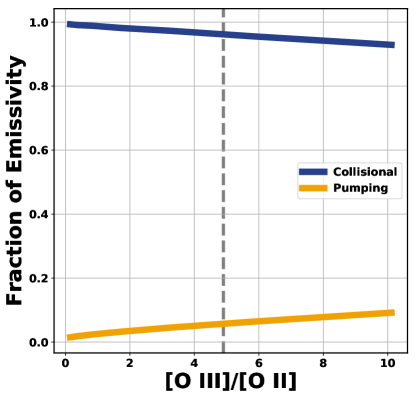
Figure 17: Plot of the fraction of the total Mg ii 2796 Å emissivity contributed by collisional excitation (blue) and photon pumping (gold) versus the [O iii] 5007 Å/[O ii] 3727 Å emission ratio from cloudy photoionization models. The dashed gray line shows the observed [O iii] 5007 Å/[O ii] 3727 Å flux ratio in J1503. The total Mg ii emissivity from galaxies with conditions similar to J1503 is dominated by collisional excitation ($>95$%).

Figure 17 uses the cloudy models to decompose the fractional impact of the total emissivity due to collisions (blue) and photon pumping of the Mg ii 2796 Å transition. cloudy does not predict other excitation mechanisms (e.g. recombination) to contribute to the Mg ii emissivity. This shows that the Mg ii emissivity is overwhelmingly ($>95$%) dominated by collisional excitation at the observed [O iii]/[O ii] values of J1503 (gray line), and photon pumping does not largely contribute to the emissivity until much higher photon densities or lower gas densities (characterized by log(U)). These cloudy models also confirm that $R_{\rm int}=2$, when collisions dominate the emissivity. This is the assumed $R_{\rm int}$ to determine $f_{\text{esc}}\left(\text{Mg\,{ii}}\right)$ throughout the paper (Equation 5).

We caution that the cloudy documentation warns that the inferred emission fluxes of resonant lines dominated by photon pumping will not include line-of-sight absorption. Therefore, cloudy will over-estimate the total contribution of photon pumping to observed resonant emission line fluxes because, in reality, absorption will decrease the transmitted flux. The contribution of photon pumping to the Mg ii emissivity will depend on the geometry of the situation (Section 16.44.3 of Hazy v17). In the geometry where the line of sight to the observer includes the continuum source, the absorption will reduce the pumping contribution to the emissivity, with the resultant line profile becoming a combination of emission plus absorption.

Appendix C The impact of the background continuum on the optical depth

In Section 6, we solved the radiative transfer equation to determine the Mg ii optical depth and column density. These Mg ii properties were combined with the gas-phase metallicity to determine $N_{\mathrm{H^{0}}}$. One simplifying assumption that we made was that the Mg ii emission was much brighter than the continuum, such that Equation 6 became

$$F_{\rm obs}=\left(F_{\rm int}+F_{\rm cont}\right)e^{-\tau}\approx F_{\rm int}e^{-\tau}.$$ (35)

However, this simplification is not necessary if the continuum can be accurately measured. If the continuum emission (F_cont), and the flux of both Mg ii emission lines is measured, Equation 35 can be turned into a system of two equations and two unknowns (where $\tau_{2803}=1/2\tau_{2796}$ and F${}_{\rm 2803,int}=1/2F_{\rm 2796,int}$ from Equation 7 and Equation 3). This system of equations can be solved, assuming that both the continuum and emission lines have the same optical depth, to give three real solutions. The only solution that leads to a positive, non-zero $\tau_{\rm 2803,cont}$ is

$$\tau_{\rm 2803,cont}=\ln{\left(\frac{F_{2803}+\sqrt{F_{2803}^{2}-F_{2796}F_{\rm cont}}}{F_{2796}}\right)}.$$ (36)

If $F_{\rm cont}=0$, this reduces to the previous $\tau_{2803}=-\ln(R/2)$ relation, given in Equation 9.

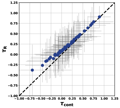
Figure 18: Plot of the optical depth calculated assuming that the Mg ii emission is much stronger than the continuum ($\tau_{R}$) versus the optical depth calculated solving the full radiative transfer equation (Equation 36). The values follow the one-to-one line over nearly the entire $\tau$ range. The values slightly deviate at low optical depth, but remain consistent within the errors. Thus, our simplification throughout the paper that $F_{\rm int}\gg F_{\rm cont}$ is valid.

Figure 18 compares the Mg ii optical depth calculated assuming that the Mg ii is much brighter than the continuum ($\tau_{\rm R}$, the value used in the paper) and explicitly accounting for the continuum attenuation ($\tau_{\rm cont}$; Equation 36). The optical depths are nearly identical for most $\tau$, and marginally deviate at the lowest $\tau$. However, the two $\tau$ values always remain statistically consistent with each other. The behavior at low optical depth is expected from Equation 36, where $F_{2803}$ must be less than $F_{2796}$ and $F_{2803}^{2}<<F_{2796}F_{\rm cont}$ to produce a low $\tau_{\rm 2803,cont}$. This indicates that $F_{\rm cont}$ impacts $\tau$ the most when the $\tau$ is low. The assumption that $F_{\rm int}\gg F_{\rm cont}$, and the subsequent results relating $R$ and $N_{\mathrm{H^{0}}}$, is valid for J1503.

References

- Alam et al. (2015) Alam S., et al., 2015, ApJS, 219, 12
- Alexandroff et al. (2015) Alexandroff R. M., Heckman T. M., Borthakur S., Overzier R., Leitherer C., 2015, ApJ, 810, 104
- Asplund et al. (2009) Asplund M., Grevesse N., Sauval A. J., Scott P., 2009, ARA&A, 47, 481
- Bañados et al. (2018) Bañados E., et al., 2018, Nature, 553, 473
- Becker et al. (2001) Becker R. H., et al., 2001, AJ, 122, 2850
- Benjamin et al. (1999) Benjamin R. A., Skillman E. D., Smits D. P., 1999, ApJ, 514, 307
- Berg et al. (2019) Berg D. A., Chisholm J., Erb D. K., Pogge R., Henry A., Olivier G. M., 2019, ApJ, 878, L3
- Borthakur et al. (2014) Borthakur S., Heckman T. M., Leitherer C., Overzier R. A., 2014, Science, 346, 216
- Burchett et al. (2020) Burchett J. N., Rubin K. H. R., Prochaska J. X., Coil A. L., Rickards Vaught R., Hennawi J. F., 2020, arXiv e-prints, p. arXiv:2005.03017
- Cai et al. (2019) Cai Z., et al., 2019, ApJS, 245, 23
- Cantalupo et al. (2014) Cantalupo S., Arrigoni-Battaia F., Prochaska J. X., Hennawi J. F., Madau P., 2014, Nature, 506, 63
- Cardelli et al. (1989) Cardelli J. A., Clayton G. C., Mathis J. S., 1989, ApJ, 345, 245
- Chisholm et al. (2018) Chisholm J., et al., 2018, A&A, 616, A30
- Chisholm et al. (2019) Chisholm J., Rigby J. R., Bayliss M., Berg D. A., Dahle H., Gladders M., Sharon K., 2019, ApJ, 882, 182
- De Barros et al. (2019) De Barros S., Oesch P. A., Labbé I., Stefanon M., González V., Smit R., Bouwens R. J., Illingworth G. D., 2019, MNRAS,
- Dijkstra et al. (2006) Dijkstra M., Haiman Z., Spaans M., 2006, ApJ, 649, 14
- Erb et al. (2012) Erb D. K., Quider A. M., Henry A. L., Martin C. L., 2012, ApJ, 759, 26
- Erb et al. (2018) Erb D. K., Steidel C. C., Chen Y., 2018, ApJ, 862, L10
- Fan et al. (2006) Fan X., et al., 2006, AJ, 132, 117
- Feltre et al. (2018) Feltre A., et al., 2018, A&A, 617, A62
- Ferland et al. (2017) Ferland G. J., et al., 2017, Rev. Mex. Astron. Astrofis., 53, 385
- Finkelstein et al. (2019) Finkelstein S. L., et al., 2019, ApJ, 879, 36
- Finley et al. (2017) Finley H., et al., 2017, A&A, 608, A7
- Fletcher et al. (2019) Fletcher T. J., Tang M., Robertson B. E., Nakajima K., Ellis R. S., Stark D. P., Inoue A., 2019, ApJ, 878, 87
- Gazagnes et al. (2018) Gazagnes S., Chisholm J., Schaerer D., Verhamme A., Rigby J. R., Bayliss M., 2018, A&A, 616, A29
- Gazagnes et al. (2020) Gazagnes S., Chisholm J., Schaerer D., Verhamme A., Izotov Y., 2020, A&A, 639, A85
- Genzel et al. (2011) Genzel R., et al., 2011, ApJ, 733, 101
- Giallongo et al. (2015) Giallongo E., et al., 2015, A&A, 578, A83
- Girard et al. (2018) Girard M., et al., 2018, A&A, 613, A72
- Girard et al. (2019) Girard M., Dessauges-Zavadsky M., Combes F., Chisholm J., Patrício V., Richard J., Schaerer D., 2019, A&A, 631, A91
- Grazian et al. (2016) Grazian A., et al., 2016, A&A, 585, A48
- Green et al. (2012) Green J. C., et al., 2012, ApJ, 744, 60
- Green et al. (2015) Green G. M., et al., 2015, ApJ, 810, 25
- Grimes et al. (2009) Grimes J. P., et al., 2009, ApJS, 181, 272
- Gronke et al. (2015) Gronke M., Bull P., Dijkstra M., 2015, ApJ, 812, 123
- Guseva et al. (2013) Guseva N. G., Izotov Y. I., Fricke K. J., Henkel C., 2013, A&A, 555, A90
- Guseva et al. (2019) Guseva N. G., Izotov Y. I., Fricke K. J., Henkel C., 2019, A&A, 624, A21
- Guseva et al. (2020) Guseva N. G., et al., 2020, arXiv e-prints, p. arXiv:2007.11977
- Hayes et al. (2014) Hayes M., et al., 2014, ApJ, 782, 6
- Heckman et al. (2011) Heckman T. M., et al., 2011, ApJ, 730, 5
- Henry et al. (2015) Henry A., Scarlata C., Martin C. L., Erb D., 2015, ApJ, 809, 19
- Henry et al. (2018) Henry A., Berg D. A., Scarlata C., Verhamme A., Erb D., 2018, ApJ, 855, 96
- Hopkins et al. (2008) Hopkins P. F., Hernquist L., Cox T. J., Kereš D., 2008, ApJS, 175, 356
- Hunter et al. (2012) Hunter D. A., et al., 2012, AJ, 144, 134
- Izotov et al. (2016a) Izotov Y. I., Schaerer D., Thuan T. X., Worseck G., Guseva N. G., Orlitová I., Verhamme A., 2016a, MNRAS, 461, 3683
- Izotov et al. (2016b) Izotov Y. I., Orlitová I., Schaerer D., Thuan T. X., Verhamme A., Guseva N. G., Worseck G., 2016b, Nature, 529, 178
- Izotov et al. (2018a) Izotov Y. I., Schaerer D., Worseck G., Guseva N. G., Thuan T. X., Verhamme A., Orlitová I., Fricke K. J., 2018a, MNRAS, 474, 4514
- Izotov et al. (2018b) Izotov Y. I., Worseck G., Schaerer D., Guseva N. G., Thuan T. X., Fricke A. V., Orlitová I., 2018b, MNRAS, 478, 4851
- Jaskot et al. (2019) Jaskot A. E., Dowd T., Oey M. S., Scarlata C., McKinney J., 2019, ApJ, 885, 96
- Jenkins (2009) Jenkins E. B., 2009, ApJ, 700, 1299
- Johnson (2019) Johnson J. A., 2019, Science, 363, 474
- Kakiichi & Gronke (2019) Kakiichi K., Gronke M., 2019, arXiv e-prints, p. arXiv:1905.02480
- Kramida et al. (2018) Kramida A., Yu. Ralchenko Reader J., and NIST ASD Team 2018, NIST Atomic Spectra Database (ver. 5.6.1), [Online]. Available: https://physics.nist.gov/asd [2019, September 3]. National Institute of Standards and Technology, Gaithersburg, MD.
- Labbé et al. (2013) Labbé I., et al., 2013, ApJ, 777, L19
- Leethochawalit et al. (2016) Leethochawalit N., Jones T. A., Ellis R. S., Stark D. P., Richard J., Zitrin A., Auger M., 2016, ApJ, 820, 84
- Leitet et al. (2011) Leitet E., Bergvall N., Piskunov N., Andersson B.-G., 2011, A&A, 532, A107
- Leitherer et al. (2014) Leitherer C., Ekström S., Meynet G., Schaerer D., Agienko K. B., Levesque E. M., 2014, ApJS, 212, 14
- Leitherer et al. (2016) Leitherer C., Hernandez S., Lee J. C., Oey M. S., 2016, ApJ, 823, 64
- Livermore et al. (2017) Livermore R. C., Finkelstein S. L., Lotz J. M., 2017, ApJ, 835, 113
- Markwardt (2009) Markwardt C. B., 2009, in Bohlender D. A., Durand D., Dowler P., eds, Astronomical Society of the Pacific Conference Series Vol. 411, Astronomical Data Analysis Software and Systems XVIII. p. 251 (arXiv:0902.2850)
- Martin et al. (2012) Martin C. L., Shapley A. E., Coil A. L., Kornei K. A., Bundy K., Weiner B. J., Noeske K. G., Schiminovich D., 2012, ApJ, 760, 127
- Martin et al. (2013) Martin C. L., Shapley A. E., Coil A. L., Kornei K. A., Murray N., Pancoast A., 2013, ApJ, 770, 41
- Matsuoka et al. (2018) Matsuoka Y., et al., 2018, ApJ, 869, 150
- Matsuoka et al. (2019) Matsuoka Y., et al., 2019, ApJ, 872, L2
- McKinney et al. (2019) McKinney J. H., Jaskot A. E., Oey M. S., Yun M. S., Dowd T., Lowenthal J. D., 2019, ApJ, 874, 52
- McMullin et al. (2007) McMullin J. P., Waters B., Schiebel D., Young W., Golap K., 2007, in Shaw R. A., Hill F., Bell D. J., eds, Astronomical Society of the Pacific Conference Series Vol. 376, Astronomical Data Analysis Software and Systems XVI. p. 127
- Mendoza (1981) Mendoza C., 1981, Journal of Physics B Atomic Molecular Physics, 14, 2465
- Michel-Dansac et al. (2020) Michel-Dansac L., Blaizot J., Garel T., Verhamme A., Kimm T., Trebitsch M., 2020, A&A, 635, A154
- Micheva et al. (2018) Micheva G., Oey M. S., Keenan R. P., Jaskot A. E., James B. L., 2018, ApJ, 867, 2
- Micheva et al. (2019) Micheva G., Christian Herenz E., Roth M. M., Östlin G., Girichidis P., 2019, A&A, 623, A145
- Morrissey et al. (2018) Morrissey P., et al., 2018, ApJ, 864, 93
- Naidu et al. (2018) Naidu R. P., Forrest B., Oesch P. A., Tran K.-V. H., Holden B. P., 2018, MNRAS, 478, 791
- Naidu et al. (2020) Naidu R. P., Tacchella S., Mason C. A., Bose S., Oesch P. A., Conroy C., 2020, ApJ, 892, 109
- Neufeld (1990) Neufeld D. A., 1990, ApJ, 350, 216
- Oesch et al. (2018) Oesch P. A., Bouwens R. J., Illingworth G. D., Labbé I., Stefanon M., 2018, ApJ, 855, 105
- Onoue et al. (2017) Onoue M., et al., 2017, ApJ, 847, L15
- Orlitová et al. (2018) Orlitová I., Verhamme A., Henry A., Scarlata C., Jaskot A., Oey M. S., Schaerer D., 2018, A&A, 616, A60
- Östlin et al. (2014) Östlin G., et al., 2014, ApJ, 797, 11
- Ott et al. (2012) Ott J., et al., 2012, AJ, 144, 123
- Ouchi et al. (2009a) Ouchi M., et al., 2009a, ApJ, 696, 1164
- Ouchi et al. (2009b) Ouchi M., et al., 2009b, ApJ, 706, 1136
- Pardy et al. (2014) Pardy S. A., et al., 2014, ApJ, 794, 101
- Prochaska et al. (2011) Prochaska J. X., Kasen D., Rubin K., 2011, ApJ, 734, 24
- Reddy et al. (2016) Reddy N. A., Steidel C. C., Pettini M., Bogosavljević M., 2016, ApJ, 828, 107
- Ricci et al. (2017) Ricci F., Marchesi S., Shankar F., La Franca F., Civano F., 2017, MNRAS, 465, 1915
- Rivera-Thorsen et al. (2019) Rivera-Thorsen T. E., et al., 2019, Science, 366, 738
- Robertson et al. (2013) Robertson B. E., et al., 2013, ApJ, 768, 71
- Robertson et al. (2015) Robertson B. E., Ellis R. S., Furlanetto S. R., Dunlop J. S., 2015, ApJ, 802, L19
- Rubin et al. (2014) Rubin K. H. R., Prochaska J. X., Koo D. C., Phillips A. C., Martin C. L., Winstrom L. O., 2014, ApJ, 794, 156
- Rupke et al. (2019) Rupke D. S. N., et al., 2019, Nature, 574, 643
- Scarlata & Panagia (2015) Scarlata C., Panagia N., 2015, ApJ, 801, 43
- Schaerer & de Barros (2010) Schaerer D., de Barros S., 2010, A&A, 515, A73
- Shapley et al. (2016) Shapley A. E., Steidel C. C., Strom A. L., Bogosavljević M., Reddy N. A., Siana B., Mostardi R. E., Rudie G. C., 2016, ApJ, 826, L24
- Shen et al. (2020) Shen X., Hopkins P. F., Faucher-Giguère C.-A., Alexander D. M., Richards G. T., Ross N. P., Hickox R. C., 2020, MNRAS, 495, 3252
- Sigut & Pradhan (1995) Sigut T. A. A., Pradhan A. K., 1995, Journal of Physics B Atomic Molecular Physics, 28, 4879
- Smit et al. (2015) Smit R., et al., 2015, ApJ, 801, 122
- Smit et al. (2018) Smit R., et al., 2018, Nature, 553, 178
- Sobral et al. (2015) Sobral D., Matthee J., Darvish B., Schaerer D., Mobasher B., Röttgering H. J. A., Santos S., Hemmati S., 2015, ApJ, 808, 139
- Steidel et al. (2011) Steidel C. C., Bogosavljević M., Shapley A. E., Kollmeier J. A., Reddy N. A., Erb D. K., Pettini M., 2011, ApJ, 736, 160
- Steidel et al. (2018) Steidel C. C., Bogosavljević M., Shapley A. E., Reddy N. A., Rudie G. C., Pettini M., Trainor R. F., Strom A. L., 2018, ApJ, 869, 123
- Swinbank et al. (2012) Swinbank A. M., Sobral D., Smail I., Geach J. E., Best P. N., McCarthy I. G., Crain R. A., Theuns T., 2012, MNRAS, 426, 935
- Swinbank et al. (2017) Swinbank A. M., et al., 2017, MNRAS, 467, 3140
- Tremonti et al. (2007) Tremonti C. A., Moustakas J., Diamond-Stanic A. a. M., 2007, ApJ, 663, L77
- Vanzella et al. (2010) Vanzella E., et al., 2010, ApJ, 725, 1011
- Vanzella et al. (2016) Vanzella E., et al., 2016, ApJ, 825, 41
- Verhamme et al. (2006) Verhamme A., Schaerer D., Maselli A., 2006, A&A, 460, 397
- Verhamme et al. (2015) Verhamme A., Orlitová I., Schaerer D., Hayes M., 2015, A&A, 578, A7
- Verhamme et al. (2017) Verhamme A., Orlitová I., Schaerer D., Izotov Y., Worseck G., Thuan T. X., Guseva N., 2017, A&A, 597, A13
- Walter et al. (2008) Walter F., Brinks E., de Blok W. J. G., Bigiel F., Kennicutt Robert C. J., Thornley M. D., Leroy A., 2008, AJ, 136, 2563
- Wang et al. (2019) Wang B., Heckman T. M., Leitherer C., Alexandroff R., Borthakur S., Overzier R. A., 2019, ApJ, 885, 57
- Weiner et al. (2009) Weiner B. J., et al., 2009, ApJ, 692, 187
- Willott et al. (2010) Willott C. J., et al., 2010, AJ, 139, 906
- Wisotzki et al. (2016) Wisotzki L., et al., 2016, A&A, 587, A98
- Worseck et al. (2014) Worseck G., et al., 2014, MNRAS, 445, 1745
- Worseck et al. (2016) Worseck G., Prochaska J. X., Hennawi J. F., McQuinn M., 2016, ApJ, 825, 144
- Zackrisson et al. (2013) Zackrisson E., Inoue A. K., Jensen H., 2013, ApJ, 777, 39
- van Zee et al. (1998) van Zee L., Skillman E. D., Salzer J. J., 1998, AJ, 116, 1186
- van Zee et al. (2001) van Zee L., Salzer J. J., Skillman E. D., 2001, AJ, 122, 121