Granular rheology: a tale of three time scales

Abstract

The law of $\mu(\mathcal{I})$ rheology has proven very successful to describe the rheology of granular liquids. It however lacks theoretical support. From the granular integration through transient formalism, we extract a simplified model that expresses the rheology of granular liquids as a competition between three time scales. In particular, this model allows to derive the $\mu(\mathcal{I})$ law within a well defined theoretical framework. Outside of the Bagnold flow regime, this framework predicts a non-trivial behavior of the effective friction coefficient. Furthermore, the extension of the model to the case of granular particles suspended in a viscous liquid provides an explanation of the similarities observed experimentally between the evolution of the friction coefficient in the suspension and the $\mu(\mathcal{I})$ law of dry granular liquids.

I Introduction

Granular fluids are omnipresent in our everyday life. The study of their behavior is important for many industrial applications, but it is also crucial to the understanding of some geological processes such as avalanches Savage (1979); Savage and Hutter (1989); Savage (1998); Pouliquen (1999); Pouliquen and Forterre (2002), pyroclastic and debris flows Kelfoun et al. (2008, 2009); Gueugneau et al. (2017); Ogburn and Calder (2017); Salmanidou et al. (2017), and sediment transport Frey and Church (2009, 2010); Pähtz et al. (2020), as well as gravisensors in plants Bérut et al. (2018); Forterre and Pouliquen (2018), and specific animal behavior Rühs et al. (2020).

Despite the absence of attractive force in the simplest granular flows, three distinct flow regimes can be identified depending on the granular fluid’s density Andreotti et al. (2013): at low density, collisions are relatively scarce, this is the gaseous regime; at higher densities — typically $0.4\lesssim\varphi\lesssim 0.6$ — the grains experience very frequent collisions, which significantly affect their qualitative behavior, this regime is called the liquid regime; finally, close to the jamming transition, interparticle friction becomes relevant with deep consequences Staron et al. (2010); DeGiuli et al. (2016); DeGiuli and Wyart (2017a, b). Most examples of granular flows on Earth are in the liquid regime Andreotti et al. (2013), this study focuses on this latter one.

When a granular liquid is in the Bagnold flow regime — which is generally the case when no external source of driving power other than shear is present — its rheology is described by a phenomenological law, called the $\mu(\mathcal{I})$ law, that has been determined by the fitting a huge data set including flows in numerous geometries GDR MiDi (2004). Since then, the $\mu(\mathcal{I})$ law has been tested against even more data, from a wide variety of flow configurations (from a simple shear experiment to the collapse of a granular column), and has shown a remarkable agreement with the experimental and numerical data both at the qualitative and the quantitative level da Cruz et al. (2005); Jop et al. (2005); Cassar et al. (2005); Jop et al. (2006); Pouliquen et al. (2006); Forterre and Pouliquen (2008); Peyneau and Roux (2008); Lagrée et al. (2011); Tankeo et al. (2013); Clavaud et al. (2017); Fullard et al. (2017); Delannay et al. (2017); Pähtz et al. (2019), even in the most recent studies Tapia et al. (2019). This formula still has one weakness however; it remains so far only phenomenological Forterre and Pouliquen (2018), the physical origin of this simple rheology has not been found out yet.

In a recent study Coquand et al. (2020), it has been shown that the Granular Integration Through Transients (GITT) formalism provides a set of fundamental equations which, once numerically solved, yield results showing a satisfactory agreement with the predictions of the $\mu(\mathcal{I})$ law, with parameter values compatible with the experimental results. Here, we show that the fundamental GITT equations can be reduced to a simpler toy-model in which the rheology of granular liquids is explained as a competition between three time scales associated to the relevant physical processes at play in the system (diffusion, shear advection and structural relaxation). This model not only allows to derive the $\mu(\mathcal{I})$ law within a theoretical framework with a well identified set of hypotheses, but also gives non-trivial predictions as for the behavior of the effective friction coefficient $\mu$ — a central rheological quantity — outside of the Bagnold regime. Furthermore, it can be easily generalized to the case of high density granular suspensions thereby providing a model for the evolution of $\mu$ in a regime where the search for such a law is under active investigation Courrech du Pont et al. (2003); Cassar et al. (2005); Boyer et al. (2011); DeGiuli et al. (2015); Guazzelli and Pouliquen (2018); Tapia et al. (2019); Pähtz et al. (2019); Suzuki and Hayakawa (2019).

The paper is organized as follows: in the first section, we present the toy-model and show that general properties of granular liquid flows can be explained through the competition between two time scales. Then, in a second section, we introduce the third time scale, derive the evolution of the effective friction coefficient, and generalize the model to granular suspensions, identifying the various flow regimes through the relative strength of the involved time scales. Finally, we conclude.

II Definition of the Toy model

Before entering the details of the toy-model, let us first recall the main properties of the GITT formalism from which it is built.

II.1 The Granular Integration Through Transients formalism

Let us consider a granular liquid consisting of $N$ infinitely hard particles, of restitution coefficient $\varepsilon$. For the sake of simplicity, we restrict ourselves to the case of an incompressible planar shear flow.

The dynamics of the system is taken to be given by the Mode-Coupling Theory (MCT), which accounts for the slow down of the relaxation of correlation functions due to the cage effect caused by clogging of particles at high density Götze (2008). The general form of the MCT equation is that of a Mori-Zwanzig equation for the dynamical structure factor $\Phi_{q}$, which is nothing but the normalized density correlation function in Fourier space: $\Phi_{q}(t)=\left<\rho_{q}(t)\rho_{-q}\right>/S_{q}$, $S_{q}=\left<\rho_{q}\rho_{-q}\right>$ being the static structure factor. The general form of this equation is given below:

$$\begin{split}\ddot{\Phi}_{q}(t)&+\nu_{q}\dot{\Phi}_{q}(t)+\Omega_{q}^{2}\Phi_{q}(t)+\Omega_{q}^{2}\int_{0}^{t}\!\!d\tau\,m_{q}(t,\tau)\dot{\Phi}_{q}(\tau)=0\>.\end{split}$$ (1)

The first three terms of Eq. (1) describe a simple relaxation of $\Phi_{q}(t)$ controlled by the two characteristic frequencies $\nu_{q}$ and $\Omega_{q}$, as for simple liquids. They express the weakening of the initial correlations through time and space. These are the terms dominating at moderate enough densities where the granular medium is in the Newtonian liquid regime. The last term accounts for the memory effects that arise when the liquid becomes supercooled, and can be expressed in the frame of the Mode-Coupling approximation. The expression of those quantities are not needed in our derivation. For details, the reader is referred to the previous papers on GITT Kranz et al. (2018, 2020); Coquand et al. (2020).

Whereas it has been shown that MCT tends to overestimate the importance of cage-effect in the vicinity of the glass transition, we are only concerned here with the dense liquid regime. In particular GITT assumes that shear-heating is always sufficient to make the granular material yield, so that we never consider a true glass phase. The regime of parameters under consideration is thus the one where the MCT has proven to provide an accurate description of the physics at play.

Given the complexity of Eq. (1), the expression of $\Phi_{q}(t)$ is not known in general, even in very simple cases. In order to understand the MCT picture of the ideal glass transition, it is useful to simplify this function thanks to the Vineyard approximation Vineyard (1958) combined with a Gaussian ansatz for the self-interacting part of the dynamical structure factor:

$$\Phi_{q}(t)\simeq S_{q}\,e^{-q^{2}\Delta r^{2}(t)}\,,$$ (2)

where $\Delta r^{2}(t)=\left<\mathbf{r}(t).\mathbf{r}(0)\right>$ is the mean-squared displacement (MSD). Hence, in the liquid phase, most particles obey a diffusive behavior of diffusion constant $D$, so that $\Delta r^{2}(t)=6Dt$, and $\Phi_{q}(t)$ shows a simple exponential relaxation (see Fig. 1). When going deeper into the supercooled regime on the other hand, the MSD develops a plateau: most particles are trapped by their neighbors and cannot escape a small region, this is the cage effect. It then follows from Eq. (2) that $\Phi_{q}(t)$ also develops a plateau (see Fig. 1). Furthermore, as long as the system is not in the ideal MCT glass phase, the plateau is followed by a final decay at later times. Note that in this picture the overall $S_{q}$ factor does not play any major role.

Finally, $\Phi_{q}(t)$ is related to rheological quantities through the Integration Through Transients (ITT) formalism Fuchs and Cates (2002, 2009), that can be used to express the shear stress $\sigma$ and the pressure $P$ in the out-of-equilibrium steady state as integrals over the values of $\Phi_{q}(t)$ at former times (see Kranz et al. (2020); Coquand et al. (2020) for more details):

$$\begin{split}&\sigma=\frac{1}{60\pi^{2}}\int_{0}^{+\infty}dt\frac{1}{\sqrt{1+\frac{(\dot{\gamma}t)^{2}}{3}}}\int_{0}^{+\infty}dq\,F_{1}(q,t)\\ &P(\dot{\gamma})=P(\dot{\gamma}=0)\\ &\quad+\frac{1}{36\pi^{2}}\int_{0}^{+\infty}dt\frac{(\dot{\gamma}t)}{\sqrt{1+\frac{(\dot{\gamma}t)^{2}}{3}}}\int_{0}^{+\infty}dq\,F_{1}(q,t)\\ &\quad+\frac{1}{12\pi^{2}}\int_{0}^{+\infty}dt\frac{(\dot{\gamma}t)}{\sqrt{1+\frac{(\dot{\gamma}t)^{2}}{3}}}\int_{0}^{+\infty}dq\,F_{2}(q,t)\,,\end{split}$$ (3)

where the kernels in the time integrals are given below:

$$\begin{split}&F_{1}(q,t)=-q^{4}\,\dot{\gamma}T\left(\frac{1+\varepsilon}{2}\right)\Phi^{2}_{q(-t)}\frac{S^{\prime}_{q(-t)}S_{q}^{\prime}}{S_{q}^{2}}\\ &F_{2}(q,t)=-q^{3}\,\dot{\gamma}T\left(\frac{1+\varepsilon}{2}\right)\Phi^{2}_{q(-t)}\frac{S^{\prime}_{q(-t)}}{S_{q}^{2}}(S_{q}^{2}-S_{q})\,.\end{split}$$ (4)

In all these expressions, the dynamical structure factor is evaluated in a time dependent wave vector $q(-t)$. This is a consequence of advection caused by the shear flow: the shear flow imposes some average motion to the particles (with a linear velocity profile in this particular case, see Fig. 2), which is antagonistic to the cage effect. The time integrals therefore reproduce the competition between the slow MCT relaxation and the shear advection.

The limit $\varepsilon\rightarrow 1$ can be taken in the above formulas to recover usual expressions in non-dissipative systems. Therefore, although we will be mostly concerned with granular flows in the following, this formalism encompasses the rheology of colloidal suspensions as a particular case.

All in all, in GITT the rheology of granular liquids is described in terms of integrals over the advected dynamical structure factor $\Phi_{q(t)}(t)$, whose dynamical evolution is described by MCT. This method has proven successful to describe the rheology of dry granular liquids Coquand et al. (2020). However, the involved structure of the equations makes it difficult to understand precisely how the underlying physical processes at play impact the end result. It is the main purpose of this paper to design a simplified version of the GITT equations that allow to recover the characteristic features of the granular rheology.

II.2 Reduction of the ITT integrals

One of the main sources of complexity in the GITT equations is the coupling between the time and wave number dependencies of $\Phi_{q}(t)$; this can be simplified. Indeed, in the MCT, the ideal glass transition is described as a bifurcation process characterized by a number of universal quantities describing the dynamics in the vicinity of the plateau of $\Phi_{q}(t)$. It is thus possible to build a class of models, called schematic models in which equivalent bifurcations apply to a function $\Phi(t)$ that is only a function of time. Consequently, the MCT equation Eq. (1) can be highly simplified, what allows for analytical studies of some of the asymptotic properties of $\Phi(t)$ when $t$ is very large. Such approach has for example been successfully applied to the rheology of colloidal suspensions Fuchs and Cates (2002, 2003); Henrich et al. (2005); Varnik and Henrich (2008); Brader et al. (2009), where it was shown that the relaxation from the plateau is dominated by the shear advection term.

However, even in the simplest schematic MCT models the full time evolution of $\Phi$ does not have a simple analytical form. Consequently, we decided in this work to go even one step further and replace $\Phi_{q}(t)$ by a simple relaxation function $\exp(-\Gamma t)$, where $1/\Gamma$ is the time scale associated with the structural relaxations, namely the scale controlling the decay of $\Phi$ to 0. In the liquid phase, $\Gamma$ is typically related to the time scales appearing in the first three terms of Eq. (1), whereas when going closer to the ideal glass transition, the memory terms are more and more important and $\Gamma\rightarrow 0$. As we will show throughout this paper, this drastic simplification is sufficient to capture the leading behavior of the system.

By taking away the $q$-dependence of $\Phi$, we also simplify all the wave vector dependences in the integrals in Eq. (3), which reduce to mere constants. However, the term appearing in the integrand is not $\Phi_{q}(t)$ but $\Phi_{q(-t)}(t)$, and although we can safely ignore the wave vector dependence of $\Phi_{q}(t)$, the effect of advection is crucial insofar as it accounts for the effect of shear which is required to liquefy the system at high densities. Hence, let us apply the Vineyard formula to $\Phi_{q(t)}(t)$ foo (a):

$$\begin{split}\Phi_{q(t)}(t)&\simeq S_{q(t)}e^{-q(t)^{2}\Delta r^{2}(t)}\\ &=S_{q(t)}e^{-q^{2}\Delta r^{2}(t)}e^{-q^{2}(\dot{\gamma}t)^{2}\Delta r^{2}(t)/3}\,.\end{split}$$ (5)

The time dependence appears on two levels: (i) in the static structure factor, but this effect is very mild and can be safely neglected at our level of approximation Henrich et al. (2007); and (ii) at the level of the Gaussian factor. The formula Eq. (5) is useful to understand the effect of shear advection on $\Phi_{q}(t)$: close to the MCT glass transition, $\Phi_{q}(t)$ develops a plateau that extends over many decades in time. However, it is not a mere function of time, it also has a spatial structure which typically decays like a Gaussian over a length given by the MSD. When the granular medium is sheared, the advection introduces an additional time-dependence in the spatial structure of $q(t)$, and therefore of $\Phi_{q(t)}(t)$. Thus, even if the MSD were constant, the large time behavior would always be $\Phi_{q}(t)\rightarrow 0$, namely, the system would be shear molten.

In our toy-model, $\Phi$ has no $q$-dependence anymore, but shear melting is required. Therefore, we choose to replace the advected $\Phi_{q(t)}(t)$ by the product of $\Phi(t)$ and a Gaussian factor $\exp(-(\dot{\gamma}t)^{2}/\gamma_{c}^{2})$, where $\gamma_{c}$ is a typical strain scale of the system. Note that this is a bit different from the choice made by Fuchs and Cates in their study of colloidal suspensions Fuchs and Cates (2003), where the advection was accounted for in the schematic model by a factor with a Lorentzian rather than Gaussian prefactor. As we are going to show in the following, the main role of the advection factor is to provide a cutoff to the time integral at a typical scale $1/\dot{\gamma}$. At our level of approximation, the precise form of this cutoff function is not important. We chose to keep the Gaussian profile because it yields simple expressions for the ITT integrals.

Finally, we can simplify the fundamental ITT integrals appearing in Eq. (3), noted $\mathcal{K}_{0}$ and $\mathcal{K}_{1}$ in the following. The fact that we reduced the $q$-dependence leads to drastic simplifications foo (b):

$$\begin{split}\mathcal{K}_{0}&=\dot{\gamma}\int_{0}^{+\infty}dt\int_{0}^{+\infty}dq\frac{F_{1}(q,t)}{\sqrt{1+(\dot{\gamma}t)^{2}/3}}\\ &\simeq\frac{\overline{\gamma}_{c}}{2}\,\frac{1}{1+u\,\overline{\gamma}_{c}}\,,\end{split}$$ (6)

where $\overline{\gamma}_{c}=\sqrt{\pi/2}\gamma_{c}$, and $u=\Gamma/\dot{\gamma}$. Similarly,

$$\begin{split}\mathcal{K}_{1}&=\dot{\gamma}\int_{0}^{+\infty}dt(\dot{\gamma}t)\int_{0}^{+\infty}dq\frac{F_{1}(q,t)}{\sqrt{1+(\dot{\gamma}t)^{2}/3}}\\ &\simeq\frac{\gamma_{c}^{2}}{4}\,\frac{1}{1+u\,\overline{\gamma}_{c}}\,.\end{split}$$ (7)

At this level of approximation, there is no major difference between the two types of ITT integrals. Details about the derivation of these formulas can be found in appendix A.

All in all, all the ITT integrals can be reduced to simple functions of a single dimensionless parameter $u$ controlled by the competition between the structural relaxation time scale $1/\Gamma$ and the shear advection time scale $1/\dot{\gamma}$.

II.3 Rheology as a competition between two time scales

Let us examine the evolution of the shear stress $\sigma$. From Eq. (3), it is basically proportional to $\mathcal{K}_{0}$. In our toy-model, it can therefore be expressed as:

$$\sigma=\frac{\sigma_{y}}{1+\overline{\gamma}_{c}\,u}\,,$$ (8)

where $\sigma_{y}$ is some constant that accounts both for the prefactor in Eq. (6), and a compensation for the $q$-dependent terms in the ITT integral. The competition between the times scales in $u$ generates different flow regimes:

• $\Gamma\gg\dot{\gamma}$: structural relaxation dominate.
  In this regime, $u\gg 1$, therefore:

  $$\sigma\simeq\frac{\sigma_{y}}{\overline{\gamma}_{c}u}=\eta\,\dot{\gamma}\,,$$ (9)

  which describes the flow of a Newtonian fluid of viscosity $\eta=\sigma_{y}/(\overline{\gamma}_{c}\Gamma)$.

  In the language of our toy-model, in this regime the shear time scale is much larger than the scale of structural relaxation. Consequently, the relaxation time depends only on the characteristic quantities of the liquid, and does not depend on the Peclet number. This behavior can be checked to show up in the numerical solution of the full GITT equations displayed in Fig. 1 in the green insert: on the left panel, the time axis is made dimensionless through the collision frequency $\omega_{c}$, all curves collapse, whereas it can be checked on the right panel, where the dimensionless time is $\dot{\gamma}t$ that different Peclet numbers are represented.

• $\dot{\gamma}\gg\Gamma$: advection dominated regime.
  Here, we must discriminate two different scenarios, because there are two separate causes that can lead the system into such a regime.

  • $\Gamma\rightarrow 0$: yielding regime.

    If $\varphi>\varphi_{g}$, where $\varphi_{g}$ is the location of the ideal MCT granular glass transition in the equivalent unsheared system Kranz et al. (2010, 2013), the structural relaxations become infinitely slow foo (c). Hence, whatever the value of $\dot{\gamma}$, the condition $u\ll 1$ is always respected. In that case,

    $$\sigma\simeq\sigma_{y}\,,$$ (10)

    which is the behavior of a yielding material of yield stress $\sigma_{y}$.

    The corresponding evolution is displayed in Fig. 1 in the red insert. Comparing the left and the right panels shows that the final relaxation time (the one corresponding to the decay of $\Phi$ to 0) is entirely determined by the Peclet number (namely by $\dot{\gamma}$), and does not depend on the collision frequency.

  • Strong shear rate regime:
    

    Even far away from the MCT granular glass transition, it is always possible to reach the regime in which $\dot{\gamma}\gg\Gamma$ if the system is sheared strongly enough. Here, we must remember that the granular medium is a dissipative system. Therefore, the existence of an out-of-equilibrium steady state requires a balance between the injected power, and the power dissipated by the medium. Whereas this balance is present in all flow regimes, in the particular case where no additional forcing is present, all the energy is injected by the shear, and dissipated by the collision, which leads to the Bagnold equation:

    $$\sigma\dot{\gamma}=\Gamma_{d}\,\omega_{c}T\,,$$ (11)

    where $\Gamma_{d}$ is a dimensionless dissipation rate (see Kranz et al. (2020) for more details). Its expression is not important here. Since $\omega_{c}\propto\sqrt{T}$, this yields $T\propto(\sigma\dot{\gamma})^{2/3}$. Then, in virtue of Eq. (3), we can write $\sigma_{y}=\hat{\sigma}_{y}T$. The equation (8), thus yields:

    $$\sigma=B\dot{\gamma}^{2}\,,$$ (12)

    where $B=\hat{\sigma}_{y}^{3}/\Gamma_{d}^{2}$ is the Bagnold coefficient of the granular fluid. Due to power balance Eq. (11), the Peclet number Pe$=\dot{\gamma}/\omega_{c}$, playing the role of a dimensionless shear rate, cannot be increased further.

    Note that while $\sigma_{y}$ has a very weak dependence on $\varepsilon$, the dissipation rate typically behaves as $\Gamma_{d}\propto(1-\varepsilon^{2})$, so that $B$ is singular in the elastic limit.

    The evolution of $\Phi_{q}$ in GITT in the Bagnold regime is represented in the blue insert in Fig. 1. As expected in an advection dominated regime, the final relaxation time is controlled by $\dot{\gamma}$.

Finally, following the reasoning of Fuchs and Cates Fuchs and Cates (2003) in the case of colloidal suspensions, we can understand the toy-model’s result Eq. (8) in the context of the viscoelastic Maxwell model. There is one subtlety related to the fact that the toy-model involves not only one, but two time scales: $\tau=1/\Gamma$ related to the structural relaxations, and $\tau_{\gamma}=\gamma_{c}/\dot{\gamma}$ related to advection. We can use them to build a total time scale $\tau_{M}$ through $1/\tau_{M}=1/\tau+1/\tau_{\gamma}$, so that Eq. (8) can be interpreted as the shear stress of a Maxwell material of shear modulus $G(t)=G_{\infty}e^{-t/\tau_{M}}$, with a short-time shear modulus $G_{\infty}$ related to the yield stress through the following Hooke’s law:

$$\sigma_{y}=G_{\infty}\overline{\gamma}_{c}\,.$$ (13)

Despite a different choice of advection term in the ITT integrals (Gaussian instead of Lorentzian), it is interesting to note that the non-linear Maxwell model of Fuchs and Cates (2003), which proved successful in the description of the rheology of colloidal suspensions, is recovered as a particular case of our toy-model (details in appendix B).

A summary of the two-time scales toy-model can be found in Fig. 1. The dominating time scale ($1/\Gamma$ or $1/\dot{\gamma}$) determines whether collisions ($u\gg 1$) or advection ($u\ll 1$) control the final decay of $\Phi(t)$ to 0. Inserts show which time scale controls the decay in three flow regimes.

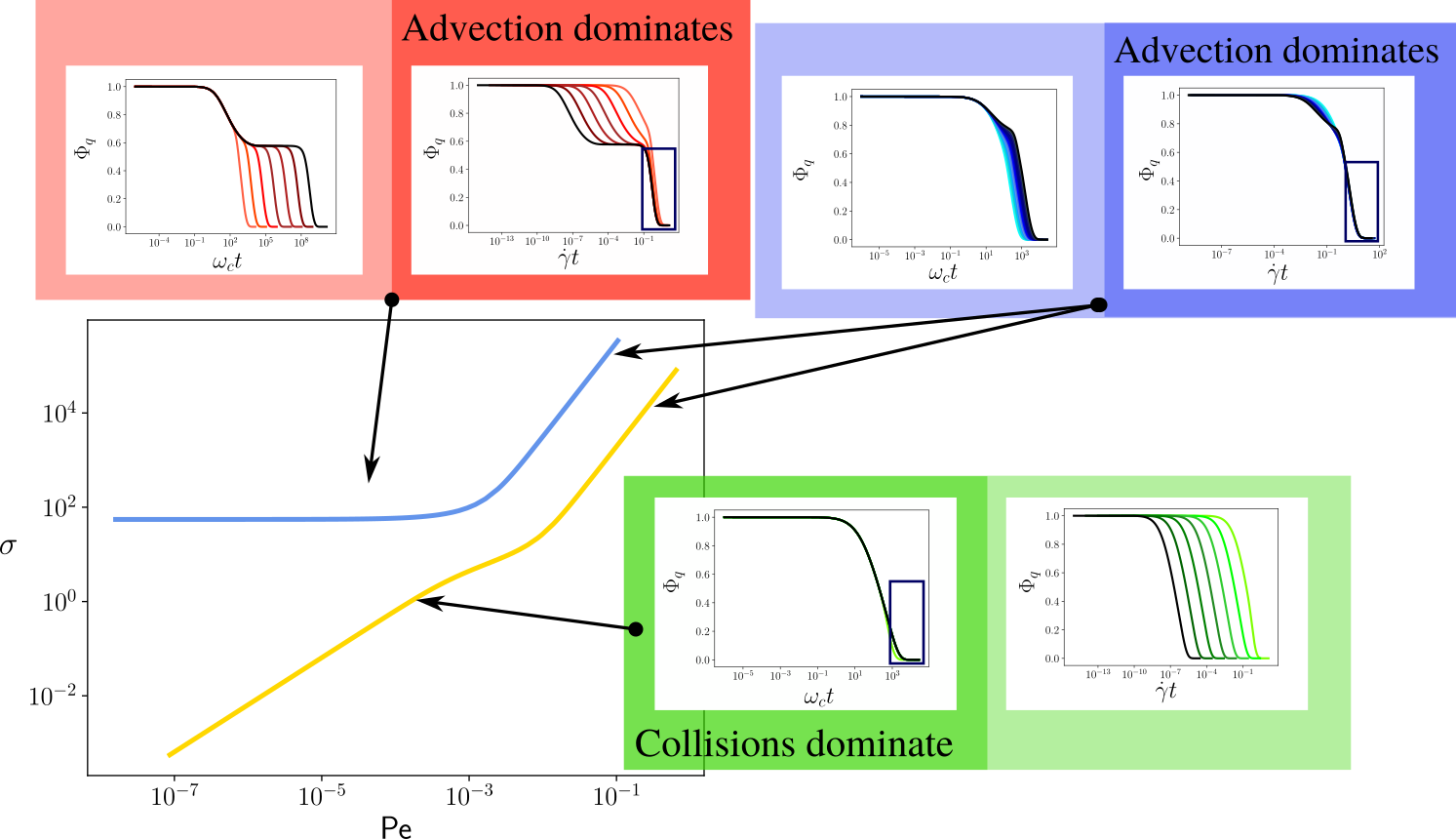
Figure 1: Evolution of the shear stress $\sigma$ as a function of the Peclet number both below the MCT granular glass transition $\varphi\leqslant\varphi_{g}$ (yellow), and above it (blue). Three inserts display the evolution of the dynamical structure factor $\Phi_{q}(t)$, computed by GITT, in the three different flow regimes (Newtonian $\sigma\propto\dot{\gamma}$ (green), yielding $\sigma\propto\dot{\gamma}^{0}$ (red), or Bagnold $\sigma\propto\dot{\gamma}^{2}$ (blue)). Each time, the left panel has a time axis rescaled by the collision frequency $\omega_{c}$ whereas it is rescaled by the shear rate $\dot{\gamma}$ on the right panel. Different curves in one insert correspond to different values of Pe. A blue rectangle indicates on which panel the different curves collapse for the final decay of $\Phi_{q}$. If the collapse is in the left panel (Newtonian regime), $\omega_{c}$ controls the decay; if it is in the right panel (yielding or Bagnold regimes), advection controls the decay.

III Effective friction

III.1 Presentation

Granular liquids are complex liquids that share some behaviors with liquids, and other with solids. A useful way to quantify how far away from these two limits the system lies, is to define its effective friction $\mu$. This coefficient, inspired from soil mechanics, describes the ability of the system to yield in a Mohr-Coulomb fashion Savage and Hutter (1989). By analogy with the Coulomb criterion of solid friction, $\mu$ is the ratio of the tangential constraint applied to the liquid over its normal constraint. In our case, it is simply $\mu=\sigma/P$. A small value of $\mu$ means that the system yields very easily, much like a liquid, whereas as $\mu$ gets closer to 1, the behavior becomes more and more solid-like.

In order to determine $\mu$ in our toy-model, we need to determine the pressure. From Eq. (3), it consists of two types of terms: the unsheared pressure $P(\dot{\gamma}=0)$ which does not depend on advection and is therefore a mere constant (denoted $P_{0}$) in our toy-model, and the ITT correction given by the two next terms (see Coquand et al. (2020) for more details). As discussed before, since the $q$-structure has been reduced to mere constant prefactors, both terms have the form of $\mathcal{K}_{1}$ given by Eq. (7). The pressure can thus be written in a form very similar to $\sigma$:

$$P=P_{0}+\frac{P_{1}}{1+\overline{\gamma}_{c}\,u}\,.$$ (14)

In particular, deep in the liquid phase in the regime dominated by $\Gamma$, the ITT correction to the pressure is very weak, whereas is goes stronger in the yielding regime, a feature consistent with the GITT numerical data Coquand et al. (2020).

Finally, the effective friction coefficient can be written as follows:

$$\mu=\frac{M_{1}}{1+M_{2}\,u}\,,$$ (15)

where $M_{1}=\sigma_{y}/(P_{0}+P_{1})$ is the limit of $\mu$ in the yielding regime and $M_{2}=\overline{\gamma}_{c}\cdot P_{0}/(P_{0}+P_{1})$. Hence, in the $\Gamma$-dominated regime, $\mu\rightarrow 0$, whereas in the yielding regime, $\mu$ reaches a constant non-zero value independent of $\dot{\gamma}$. This is all the more interesting as it has been shown that pyroclastic flows have a much lower $\mu$ than typical values predicted by the $\mu(\mathcal{I})$ law. Indeed, some processes have been suggested to explain that such flow are not in the Bagnold regime where the $\mu(\mathcal{I})$ law applies Gueugneau et al. (2017). Our toy-model confirms that some parameter ranges (corresponding to the Newtonian flow regime) are compatible with arbitrarily low values of $\mu$.

The predictions of the toy-model can be tested against the evolution of $\mu$ with the Peclet number Pe $=\dot{\gamma}/\omega_{c}$ computed with GITT (see Fig. 2). The following behavior is observed in the numerical data: for $\varphi\leqslant\varphi_{g}$, $\mu$ asymptotically goes to 0 when Pe decreases, whereas it saturates to a finite value around $0.4$ for $\varphi>\varphi_{g}$. This is consistent with the prediction of the toy-model: below the MCT granular glass transition, $\Gamma$ is finite, and when decreasing Pe, it is always possible to reach the regime $\Gamma\gg\dot{\gamma}$ where $\mu$ can be arbitrarily small; above $\varphi_{g}$ however, the structural relaxations become infinitely slow, and the system stays in the yielding regime where $u\ll 1$. At this order of approximation, our two-time-scales toy-model therefore reproduces exactly the behavior observed in GITT.

This result is a bit disturbing though since it means that in the yielding regime, $\mu$ does not depend on $u$. While this seems satisfactory at lowest order, as can be seen in Fig. 2, when looking at individual curves like in Fig. 3, $\mu$ clearly depends on Pe even in the yielding regime, even if its variations are much milder (they are all the weaker that $\varphi$ is large).

The origin of this is easy to understand: in the GITT curves, the behavior of $\mu$ is studied when Pe $\rightarrow 0$. In the Newtonian regime, $\Gamma\propto\omega_{c}$, so that Pe $\propto 1/u$ and the identification between the toy-model and the GITT data is easy to make. In the yielding regime however, $u\ll 1$ whatever small Pe is. This is because in this regime, the plateau in the time evolution of $\Phi$ is very long (see the upper-left quadrant on Fig. 2), the internal dynamics is very slow due to a strong cage effect, and the condition $\Gamma\ll\dot{\gamma}$ can be maintained even at very low values of $\dot{\gamma}$. The identification between $u$ and Pe therefore breaks down in this regime. Indeed, as pinpointed in Coquand et al. (2020), the rheology of granular liquids is not defined in terms of one, but two dimensionless ratios of time scales: the Peclet number Pe, and the Weissenberg number Wi $=\dot{\gamma}/\Gamma$.

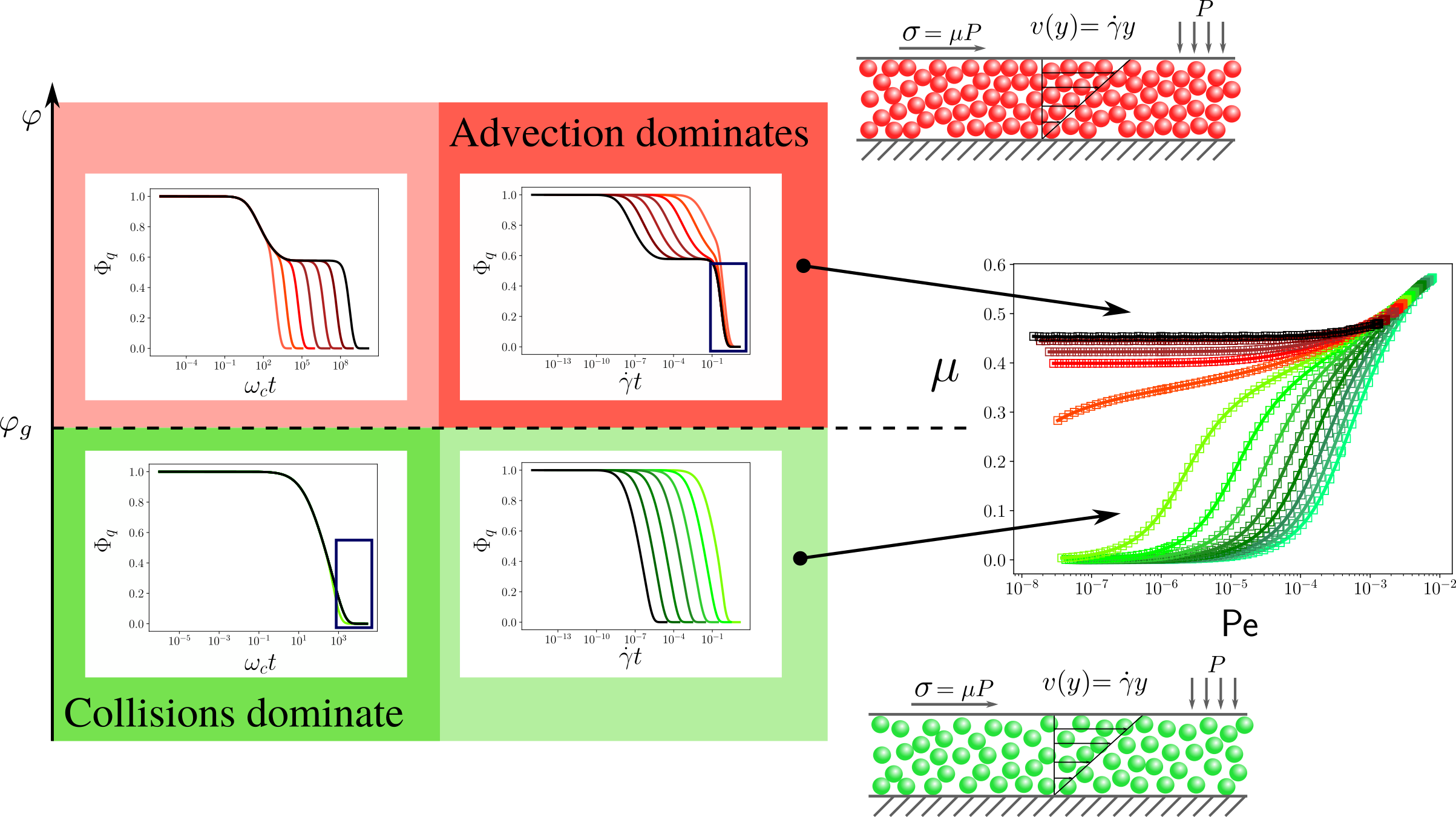
Figure 2: The left part of the figures recalls the shape of the dynamical structure factor’s evolution with time. On the left panel, the time axis is rescaled by $\omega_{c}$, whereas on the right panel, it is rescaled by $\dot{\gamma}$. This allows to identify the process that controls the decay of $\Phi_{q}$: collisions under the MCT granular glass transition (at $\varphi=\varphi_{g}$), and advection above. On the right side, the flow geometry is recalled, and the evolution of $\mu$ with Pe is displayed for various values of $\varphi$. Depending on the process controlling the decay of $\Phi_{q}$, the Pe $\rightarrow 0$ limit of $\mu$ is either 0 or a finite value.

III.2 The three-time-scales rheology

As stated before, the rheology of granular liquids depends on two dimensionless numbers: Pe that describes the competition between diffusion and advection, and Wi that in that case describe the competition between cage effect and advection. A consequence of the existence of three fundamental time scales — for diffusion, advection, and structural relaxations — can be seen on the time evolutions of $\Phi_{q}(t)$ (see Fig. 1 and Fig. 2). In the Newtonian regime, the cage effect is weak, most of the physics is captured by the competition between diffusion and advection, and $\Phi_{q}(t)$ follows a simple decay. Closer to the MCT granular glass transition, the time scales associated to diffusion and structural relaxations separate and $\Phi_{q}(t)$ follows a two-step decay.

Changing from a one-step to a two-step decay can be done simply by assuming that $\Phi(t)$ does not follow a simple exponential relaxation, but is rather a combination of two such processes: $\Phi(t)=\lambda^{(1)}\exp(-\Gamma^{(1)}t)+\lambda^{(2)}\exp(-\Gamma^{(2)}t)$, with $\Gamma^{(1)}$ associated to the short-time diffusion process, whereas $\Gamma^{(2)}$ is associated to the long-time decay process. By linearity of the ITT integrals foo (d), it can be checked that the resulting shear stress can be decomposed as $\sigma=\sigma^{(1)}+\sigma^{(2)}$, each $\sigma^{(i)}$ having the form Eq. (8), with two respective time scales ratios $u^{(i)}=\Gamma^{(i)}/\dot{\gamma}$. Following the above discussion, $u^{(1)}\propto 1/$Pe and $u^{(2)}\propto 1/$Wi. The same procedure can be applied to $P$ and to $\mu$.

The success of the two-time scales toy-model hints that the long-time relaxation process is associated with the more drastic variations of the rheological quantities (such as the shift from a $\mu\rightarrow 0$ limit to a finite value of $\mu$ when Pe $\ll 1$). In the cases where the decay of $\Phi$ is done in two well separated steps, the changes associated to the first step of the decay are milder, subleading variations.

We therefore split $\mu$, in this fashion, introducing two separate contributions $\mu^{(1)}$ and $\mu^{(2)}$ coming respectively from the short and the long time scales controlling the decays,

$$\mu=\mu^{(1)}+\mu^{(2)}=\frac{M_{1}^{(1)}}{1+M_{2}^{(1)}\,u^{(1)}}+\frac{M_{1}^{(2)}}{1+M_{2}^{(2)}\,u^{(2)}}\,.$$ (16)

As can be seen in Fig. 2, the short-time decay is completely fixed by $\omega_{c}$, and $u^{(1)}\propto 1/$ Pe. In the yielding regime, the long-time decay becomes infinitely large, so that $u^{(2)}=0$. Our previous paradox is therefore solved: $\mu$ does possess a contribution from yielding that stays constant and fixes the leading behavior, but it also encompasses a second term, due to the short-time decay, which is still of form Eq. (15), and explains the remaining subleading variation.

This model is tested against GITT data in Fig. 3. In the Newtonian regime, the two time scales collapse on each other, $u^{(1)}=u^{(2)}$, and $\mu$ has the form of Eq. (15). When going closer to the ideal granular glass transition, the two time scales separate, as in Fig. 2, and $\mu^{(2)}$ gets closer to a constant, while $\mu^{(1)}$ still depends on Pe. Fitting the GITT data with such a model yields the red curves in Fig. 3. The agreement between the numerical data and the model is satisfactory.

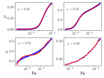
Figure 3: Evolution of $\mu$ with Pe computed numerically with GITT (blue circles). The red curve is the result of the fitting of the data with our toy-model Eq. (16).

III.3 The $\mu(I)$ regime

In the previous section, we did not discuss the last regime of dry granular flows: the Bagnold regime. In this regime it has been established experimentally that $\mu$ follows a phenomenological law, and depends on only one dimensionless quantity, the inertial number $\mathcal{I}=\dot{\gamma}d\sqrt{n/P}$ — $n$ being the particle’s density and $d$ their diameter — which can be understood as the ratio of two time scales Cassar et al. (2005): the advection time scale $t_{\gamma}=1/\dot{\gamma}$, and the time scale of free-fall in a pressure field $P$, $t_{ff}$ , which is the characteristic scale of the ballistic short time motion. The $\mu(\mathcal{I})$ law writes:

$$\mu(\mathcal{I})=\mu_{1}+\frac{\mu_{2}-\mu_{1}}{1+\mathcal{I}_{0}/\mathcal{I}}\,,$$ (17)

where $\mathcal{I}_{0}$, $\mu_{1}$ and $\mu_{2}$ are adjustable parameters. This law has been tested in a wide variety of flow geometries GDR MiDi (2004); Lagrée et al. (2011); Pähtz et al. (2020), and has proven to be successful, even in very recent experiments Forterre and Pouliquen (2018); Tapia et al. (2019). This is crucial insofar as it means that the law Eq. (17) provides knowledge about intrinsic properties of granular liquids.

Let us examine the $\mu(\mathcal{I})$ law in the light of our toy-model. As explained before, in the Bagnold regime, the shear rate is strong enough so that the system lies in the advection dominated regime $u\ll 1$. Therefore the long time scale ratio $u^{(2)}$ is very small, and the contribution $\mu^{(2)}$ is roughly constant. This is consistent with the fact that in typical experiments, the variation of $\mu$ over the whole $\mathcal{I}$ range is mild — it typically varies between $0.4$ and $0.65$. The subleading variations thus come from the change of short-time decay scale, that can be observed in Fig. 1.

By definition, $u^{(1)}$ is the ratio of the time scale associated with the short-time motion of the particle, which in this case can be identified with $t_{ff}$. Therefore, $u^{(1)}\propto 1/\mathcal{I}$.

Let us now examine a bit more in details the different regimes. The behavior of the system is controlled by three independent time scales: the advection time scale $t_{\gamma}$, the free fall time scale $t_{ff}$, and the scale of the structural relaxations $t_{\Gamma}$. In the Bagnold regime, the final relaxation is always controlled by advection, therefore $t_{\gamma}\ll t_{\Gamma}$. Hence, three different regimes can be defined depending on the values of $t_{ff}$:

• $t_{ff}\ll t_{\gamma}\ll t_{\Gamma}$: Quasi-static regime.
  In this regime, $t_{ff}$ is the smallest time scale, $\mathcal{I}=t_{ff}/t_{\gamma}\ll 1$. From what we established before, $u^{(2)}\ll 1$ and $u^{(1)}\gg 1$. The effective friction, given by Eq. (16) is thus dominated by the long-time contribution $\mu^{(2)}$. By analogy with Eq. (17), we can identify,

  $$\mu\simeq\mu^{(2)}\simeq M_{1}^{(2)}=\mu_{1}\,.$$ (18)

  This corresponds to the black curve in Fig. 2, where the two relaxation time scales are clearly separated.

  Let us emphasize that our result only hold for moderately low values $\mathcal{I}\gtrsim 10^{-3}$, beyond that interparticle friction plays the dominant role, and defines the physics of the jamming transition Staron et al. (2010); DeGiuli et al. (2015, 2016); DeGiuli and Wyart (2017b).

• $t_{\gamma}\simeq t_{ff}\ll t_{\Gamma}$: $\mu(\mathcal{I})$ regime.
  This is the regime where $\mu$ varies between its two limiting values $\mu_{1}$ and $\mu_{2}$. In this regime, the two relaxation time scales get closer and closer to each other until they finally merge into one. The decay of $\Phi$ is controlled by $t_{ff}\simeq t_{\gamma}$.

• $t_{\gamma}\ll t_{ff}\simeq t_{\Gamma}$: Dilute liquid limit.
  In the limit of the lowest packing fractions accessible to the granular liquid phase, the advection time scale becomes even smaller than the internal relaxation time scale. In such a regime, both $u^{(1)}\ll 1$ and $u^{(2)}\ll 1$. Comparing the toy-model $\mu$ Eq. (16) and the experimental law Eq. (17) leads to:

  $$\mu\simeq M_{1}^{(1)}+M_{1}^{(2)}=\mu_{2}\,,$$ (19)

  which together with Eq. (18) leads to $M_{1}^{(1)}=\mu_{2}-\mu_{1}$.

Finally, defining $\mathcal{I}_{0}=M_{2}^{(1)}\,u^{(1)}\,\mathcal{I}$,

$$\mu^{(1)}=\frac{\mu_{2}-\mu_{1}}{1+\mathcal{I}_{0}/\mathcal{I}}\,,$$ (20)

so that recalling that in the Bagnold regime $u^{(2)}\ll 1$ is always true, this equation combined with Eq. (18) show that Eq. (16) is exactly equivalent to Eq. (17).

It is also interesting to interpret the above results in terms of Maxwell’s model. Since $\sigma=\int dt\dot{\gamma}G(t)$, we can identify $G(t)$ with $\Phi(t)^{2}$, which leads to the following equation for the time dependent shear modulus:

$$G(t)=\left[(G_{0}-G_{\infty})e^{-2\Gamma^{(1)}t}+G_{\infty}e^{-2\Gamma^{(2)}t}\right]e^{-(\dot{\gamma}t)^{2}/\gamma_{c}^{2}}\,,$$ (21)

where, recalling that $G(t)$ follows a two-step decay similar to that of $\Phi(t)$, $G_{0}$ is the initial value of the shear modulus, and $G_{\infty}$ that of the plateau $1/\Gamma^{(1)}\ll t\ll 1/\Gamma^{(2)}$. Accordingly, $G_{0}\geqslant G_{\infty}$. This model differs from the above non-linear Maxwell model because of two features: (i) it is expressed in terms of not only one but two characteristic shear moduli, which allows for a richer phenomenology, and (ii) the contribution of the advection time $\tau_{\gamma}=\gamma_{c}/\dot{\gamma}$ is now quadratic instead of linear. Consequently, the shear stress can be written:

$$\sigma=\frac{\sigma_{y}\left(\frac{G_{0}}{G_{\infty}}-1\right)}{1+\overline{\gamma}_{c}u^{(1)}}+\frac{\sigma_{y}}{1+\overline{\gamma}_{c}u^{(2)}}\,,$$ (22)

where $\sigma_{y}$ and $G_{\infty}$ are related by Eq. (13). The pressure can also be decomposed:

$$P=P_{0}+\frac{P_{1}}{1+\overline{\gamma}_{c}u^{(1)}}+\frac{P_{2}-P_{1}}{1+\overline{\gamma}_{c}u^{(2)}}\,,$$ (23)

what finally leads to the following expressions for $\mu_{1}$ and $\mu_{2}$:

$$\mu_{1}=\frac{G_{\infty}\overline{\gamma}_{c}}{P_{0}+P_{1}}\ ,\ \mu_{2}=\frac{G_{0}\overline{\gamma}_{c}}{P_{0}+P_{2}}\,.$$ (24)

Hence, $\mu_{1}$ corresponds to the plateau elastic response of the viscoelastic fluid, whereas $\mu_{2}$ is associated with its initial value before the first step of the decay. Consistently with $G_{0}\geqslant G_{\infty}$, $\mu_{1}\leqslant\mu_{2}$ always holds.

Finally, the identification of $\mu_{1}$ and $\mu_{2}$ with the model of $\dot{\gamma}$-dependent friction of Savage and Hutter Savage and Hutter (1989) (see details in appendix C) allows us to identify $\mu_{1}=\tan(\delta_{S})$ and $\mu_{2}=\tan(\delta_{D})$, where $\delta_{S}$ and $\delta_{D}$ that delimit the regime in which steady shear flow can develop down slopes.

All in all, the $\mu(\mathcal{I})$ law is recovered as a particular case of our toy-model. It is deduced from the fundamental equation Eq.(16) by the additional constraint that in the Bagnold regime the final relaxation process is always controlled by shear advection, in which case $\mu^{(2)}$ is a mere constant. It was discussed in a previous studies Peyneau and Roux (2008); Clavaud et al. (2017); Pähtz et al. (2020); Coquand et al. (2020) that $\mu_{1}$ was not related to the interparticle friction, but arose rather from collective effects. What the present study adds to this picture is the relation between the non-zero value of $\mu_{1}$ and the separation of time scales in the relaxation of $\Phi$ towards 0.

III.4 Granular suspensions

In a series of recent studies, striking similarities between the laws governing the flow of dry granular liquids and granular suspensions Courrech du Pont et al. (2003); Cassar et al. (2005); Boyer et al. (2011); DeGiuli et al. (2015); Guazzelli and Pouliquen (2018); Tapia et al. (2019); Pähtz et al. (2019); Suzuki and Hayakawa (2019). For the sake of consistency, let us let aside the considerations about the regime close to the jamming transition DeGiuli et al. (2015); Tapia et al. (2019), and focus on the dense liquid regime.

The main results can be summarized as follows: in presence of a viscous liquid, a new time scale related to the steady motion of particles submitted to a drag force proportional to its velocity, called $t_{\eta}$, must be taken into account Courrech du Pont et al. (2003); Cassar et al. (2005); foo (e). The ratio of this time scale and the advection time scale defines a new dimensionless number $\mathcal{J}=\eta_{\infty}\dot{\gamma}/P$ foo (f), where in accordance with our previous notations $\eta_{\infty}$ is the viscosity of the surrounding fluid.

It was then observed that $\mu$ follows a law, similar to Eq. (17), but where $\mathcal{J}$ rather than $\mathcal{I}$ plays the role of dimensionless number. More precisely, it was proposed in Boyer et al. (2011) that $\mu(\mathcal{J})$ writes in the following form:

$$\begin{split}\mu(\mathcal{J})&=\mu^{c}(\mathcal{J})+\mu^{h}(\mathcal{J})\\ &=\mu_{1}+\frac{\mu_{2}-\mu_{1}}{1+\mathcal{I}_{0}/\mathcal{J}}+\mu^{h}(\mathcal{J})\,.\end{split}$$ (25)

In the above expression two kinds of terms are identified: a collisional contribution which form is very similar to Eq. (17), and a hydrodynamic term that is tailored to reproduce Einstein’s viscosity at low density.

Let us examine this result in the light of our toy-model. As explained above, the main effect of the surrounding fluid is to introduce a new time scale $t_{\eta}$ that will compete with $t_{ff}$, $t_{\Gamma}$ and $t_{\gamma}$ to determine the leading behavior of $\mu$.

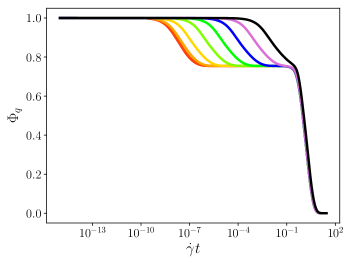
Figure 4: Dynamical structure factor of granular suspensions for Pe=$10^{-9}$, $\varphi=0.58$ and Pe₀ between $2.10^{-5}$ (red) and $2.10^{3}$ (black) obtained as a numerical solution of the GITT equations. The curves for Pe${}_{0}<10^{-5}$ all collapse on the red one.

A good way to understand how the various time scales relate to each other is to first look at the numerical data from GITT. On Fig. 4 are displayed various profiles of $\Phi$. In order to visualize better the effect of $t_{\eta}$, which is a short-time scale, we choose a high $\varphi$ and a very low $\dot{\gamma}$, so that the long-time decay is delayed as much as possible. Two main regimes can be distinguished: if the Peclet number of the surrounding fluid Pe${}_{0}=\dot{\gamma}d^{2}/D$ — $D$ being the diffusion coefficient in this fluid — is small enough, all curves collapse as far as the first step of the decay is concerned, namely the first step of the decay is controlled by $\omega_{c}$ independent of the presence or absence of bathing fluid. This is the dry granular liquid regime studied before, that extends to suspensions in a fluid with a low enough $\eta_{\infty}$. Then, for higher Pe₀’s, $t_{\eta}$ determines the scale associated to the first decay until it merges with $t_{\Gamma}$. This is the viscous suspension regime.

Short-time decay	Long-time decay	Flow regime
Dry granular liquid:   $t_{\eta}\ll t_{ff}$	$t_{\gamma}\gg t_{\Gamma}$	$t_{\Gamma}\simeq t_{ff}$: Newtonian
		$t_{\Gamma}\gg t_{ff}$ : Strongly coupled
	$t_{\Gamma}\gg t_{\gamma}$	$t_{\gamma}\gg t_{ff}$ : Quasi-static
		$t_{\gamma}\simeq t_{ff}$ : Dense liquid
		$t_{\gamma}\ll t_{ff}$ : Dilute liquid
Granular suspension:      $t_{\eta}\gg t_{ff}$	$t_{\gamma}\gg t_{\Gamma}$	$t_{\Gamma}\simeq t_{\eta}$: Newtonian
		$t_{\Gamma}\gg t_{\eta}$ : Strongly coupled
	$t_{\Gamma}\gg t_{\gamma}$	$t_{\gamma}\gg t_{\eta}$ : Quasi-static
		$t_{\gamma}\simeq t_{\eta}$ : Dense liquid
		$t_{\gamma}\ll t_{\eta}$ : Dilute viscous

Table 1: Summary of the different regimes determined by the various time scales in granular suspensions.

A summary of all the different regimes accessible to the system is given in Tab. 1. There are four competing time scales, but not all possible combinations are allowed. The short time decay is controlled either by $t_{\eta}$ or $t_{ff}$. When the liquid is Newtonian, which corresponds to memory effects playing a negligible role in the MCT equation Eq. (1), the short-time scale is equal to $t_{\Gamma}$. Note that by definition, $t_{\Gamma}\geqslant t_{\eta},t_{ff}$.

If $t_{\Gamma}\ll t_{\gamma}$, the long-time decay is independent of advection. Thus, the liquid can be either Newtonian, or strongly coupled if the density is high enough so that the cage effect becomes important and the two relaxation scales separate from each other.

The remaining regimes are the regimes controlled by advection, which can be either Bagnold or yielding. In the case $t_{\eta}\ll t_{ff}$, the $\mu(\mathcal{I})$ rheology is recovered. If $t_{\eta}\gg t_{ff}$ on the other hand, the short-time decay is determined by $\eta_{\infty}$. By a reasoning similar to the one we used previously, the ratio $u^{(1)}$ in Eq. (16) is thus $u^{(1)}\propto 1/\mathcal{J}$. This explains the strong similarities between the functional form of $\mu$ in the dry and suspended cases: what changes is simply the nature of the short-time scale; $\mu$ is still determined in the same fashion by the competition of a two-step decay profile, and advection.

For example, let us consider the case of a dense granular suspension in the Bagnold regime. Strictly speaking, adding a viscous fluid changes the Bagnold equation since motion in the liquid adds a new source of energy dissipation in the system. However, the power dissipated by Stokes’ force scales as $T$, whereas the power dissipated by collisions scales as $T^{3/2}$. Therefore, at high enough density, we can reasonably expect that collisions are the primary source of energy dissipation. Hence, the large time contribution $\mu^{(2)}$ should be unchanged compared to the dry case, that is: $\mu^{(2)}=\mu_{1}$. As for $\mu^{(1)}$, the only change is the nature of $u^{(1)}$ which is now $\propto 1/\mathcal{J}$. All in all,

$$\mu=\mu_{1}+\frac{\mu_{2}-\mu_{1}}{1+\mathcal{J}_{0}/\mathcal{J}}\,,$$ (26)

where $\mathcal{I}_{0}$ has been changed into $\mathcal{J}_{0}$ to account for the fact that the factor relating $u^{(1)}$ to $1/\mathcal{I}$ or $1/\mathcal{J}$ may differ; but the other coefficients are unchanged. In particular, in Eq. (26) only the collisional part $\mu^{c}$ contributes. This is consistent with the experimental findings of Cassar et al. (2005). It also means that the value of $\mu$ in the quasi-static limit should be the same in the dry and the suspended cases, which is also consistent with experiments Cassar et al. (2005); Guazzelli and Pouliquen (2018); Tapia et al. (2019); foo (g).

When going away from this particular case, $\mu^{(2)}$ acquires a non-trivial structure which should account for $\mu^{h}$ foo (h). We cannot however test our model against the particular form of $\mu^{h}$ used in Boyer et al. (2011) because (i) our toy-model expresses everything in terms of ratios of time scales, whereas Boyer et al. (2011) fits a known $\varphi$-dependent function, and (ii) there is no guarantee that the low $\varphi$ limit of our model, built to be precise for $\varphi\gtrsim 0.4$, has the Einstein’s viscosity as a natural limit as this expression is expected to be precise only up to $\varphi\simeq 0.03$ Petford (2009).

Finally, an important feature of non-Brownian suspensions by opposition to dry granular liquids is the dilute liquid limit in which $\mu$ saturates in dry liquids, but continues to increase in suspensions Boyer et al. (2011). This goes a little bit beyond the frame of our model insofar as the regime in which $\mu$ really saturates is rarely reached by experiments, which means that the dense-liquid approach may break down before $\mu$ saturates, and the remaining variations can be accounted for by the difference between $\mathcal{I}_{0}$ and $\mathcal{J}_{0}$. Indeed, whereas in dry granular liquids when $\varphi$ is sufficiently decreased the stress is not well transmitted through the whole fluid, in the case of suspensions in a viscous enough liquid, the surrounding fluid can carry the stress to all particles and maintain the average velocity profile. Therefore, it is not even clear that the validity of our approach in the dilute limit extends to the same boundaries in the dry and suspended cases.

IV Conclusion

All in all, we have shown that most of the rheology of granular liquids can be explained by a competition between fundamental time scales. A first two-time scales version of the toy-model, based on the competition between structural relaxations and advection successfully explains the main features of the rheology, such as the behavior of $\sigma$ in the different flow regimes, the viscoelastic properties of the liquid, and the bifurcation separating a small $\mu$ to a finite $\mu$ limit when $\varphi$ is varied. The addition of a third time scale in the diffusion-advection-structural relaxation toy-model allows to account for additional milder variations of the rheological parameters, and explain the $\mu(\mathcal{I})$ law. Furthermore, the understanding of the physics as a competition between the time scales controlling both the first and the second steps of the decays of $\Phi$ yields a generalization of the model to the case of granular suspensions, where it gives predictions as for the values of the hydrodynamic contribution to the effective friction.

Appendix A Reduction of the ITT integrals

This appendix contains some details on the derivation of Eq. (6) and Eq. (7).

First, we implement the approximation of the toy-model: we replace $\Phi_{q}(t)$ by an exponential decay, and add the advection Gaussian factor:

$$\begin{split}\mathcal{K}_{0}&=\dot{\gamma}\int_{0}^{+\infty}dt\int_{0}^{+\infty}dq\frac{F_{1}(q,t)}{\sqrt{1+(\dot{\gamma}t)^{2}/3}}\\ &\simeq\dot{\gamma}\int_{0}^{+\infty}dt\,e^{-2\Gamma t-2(\dot{\gamma}t)^{2}/\gamma_{c}^{2}}\\ &=\frac{\gamma_{c}\sqrt{\pi}}{2\sqrt{2}}\,e^{\Gamma^{2}\gamma_{c}^{2}/(2\dot{\gamma}^{2})}\text{erfc}\left(\frac{\Gamma\gamma_{c}}{\dot{\gamma}\sqrt{2}}\right)\,.\end{split}$$ (27)

Rigorously speaking, $\mathcal{K}_{0}$ includes an additional overall factor that accounts for the wave number integral.

Then, we can replace $\exp(x^{2})\text{erfc}(x)$ by $1/(1+x\sqrt{\pi})$ that shares the same $x\ll 1$ and $x\gg 1$ behaviors at leading order, and represents a satisfactory approximation of the whole function (see Fig. 5), which gives

$$\mathcal{K}_{0}\simeq\frac{\overline{\gamma}_{c}}{2}\,\frac{1}{1+\overline{\gamma}_{c}\,u}\,.$$ (28)

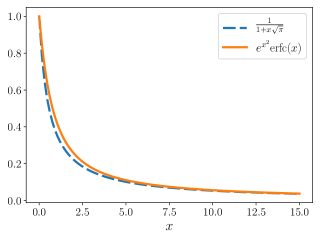
Figure 5: Comparison of the functions $x\mapsto 1/(1+x\sqrt{\pi})$ (dashed line) and $x\mapsto e^{x^{2}}\text{erfc}(x)$ (full line).

The second ITT integrals appears in the expression of the correction to the pressure due to the shear foo (i):

$$\begin{split}\mathcal{K}_{1}&=\dot{\gamma}\int_{0}^{+\infty}dt(\dot{\gamma}t)\int_{0}^{+\infty}dq\frac{F_{1}(q,t)}{\sqrt{1+(\dot{\gamma}t)^{2}/3}}\\ &\simeq\frac{\gamma_{c}^{2}}{4}\left(1-\overline{\gamma}_{c}\,u\,e^{u^{2}\gamma_{c}^{2}/2}\text{erfc}\left(u\,\gamma_{c}/\sqrt{2}\right)\right)\,.\end{split}$$ (29)

At this stage, the first option is to apply the same approximation as for $\mathcal{K}_{0}$, which gives the formula Eq. (7).

However, using this replacement for $\mathcal{K}_{1}$ is not as precise as it was for $\mathcal{K}_{0}$. Indeed, when $u\gg 1$, the two leading order terms in the expression Eq. (29) cancel against each other, so that $\mathcal{K}_{1}$ is $O(1/u^{2})$, and not $O(1/u)$ as predicted by Eq. (7).

A better approximation can be built by relating $\mathcal{K}_{1}$ to $\mathcal{K}_{0}$:

$$\begin{split}\mathcal{K}_{1}&\simeq\dot{\gamma}\int_{0}^{+\infty}dt(\dot{\gamma}t)\,e^{-2\Gamma t-2(\dot{\gamma}t)^{2}/\gamma_{c}^{2}}\\ &=-\frac{\dot{\gamma}}{2}\frac{d}{d\Gamma}\left(\int_{0}^{+\infty}dt\,e^{-2\Gamma t-2(\dot{\gamma}t)^{2}/\gamma_{c}^{2}}\right)\\ &=-\frac{\dot{\gamma}}{2}\frac{d\mathcal{K}_{0}}{d\Gamma}\\ &=\frac{\overline{\gamma}_{c}^{2}}{4}\frac{1}{(1+\overline{\gamma}_{c}\,u)^{2}}\,.\end{split}$$ (30)

This expression can be used to replace Eq. (7) throughout the reasoning presented in this article. It yields higher order terms with higher powers of $\mathcal{I}$ in the $\mu(\mathcal{I})$ law.

Given the excellent agreement between the $\mu(\mathcal{I})$ law and the available experimental data, we preferred to keep the simpler Eq. (7) in our derivation. However, this computation reminds us that this law is only approximate.

Appendix B The non-linear Maxwell model

In their study of the rheology of colloidal suspensions Fuchs and Cates (2003), Fuchs and Cates designed a simple toy-model which reproduces the ability of the complex colloidal liquid to interpolate between the Newtonian and the yielding regimes. In the Maxwell model of viscoelastic fluids in which the shear rate is decomposed into a solid-like and a liquid-like contributions, it can be established that the dynamical shear modulus $G(t)$ follows an evolution of type $G(t)=G_{\infty}e^{-t/\tau}$. In colloidal suspensions, as in the case of granular fluids, there are two characteristic time scales in competition: the structural relaxation time scale $\tau$, and the advection time scale $\tau_{\gamma}=c/\dot{\gamma}$ ($c$ being an unimportant constant). Fuchs and Cates then proposed to replace the time scale in the Maxwell model of viscoelasticity by $\tau_{M}$ defined as:

$$\frac{1}{\tau_{M}}=\frac{1}{\tau}+\frac{1}{\tau_{\gamma}}\,,$$ (31)

what leads to the following expression for the shear stress:

$$\sigma=\dot{\gamma}\left(\eta_{\infty}+\frac{G_{\infty}\,\tau}{1+\dot{\gamma}\tau/c}\right)\,,$$ (32)

where $\eta_{\infty}$ is the viscosity of the surrounding fluid.

The interpretation of Eq. (32) goes as follows: at low density, $\dot{\gamma}\tau\ll 1$, so that $\sigma\simeq\eta_{\infty}\dot{\gamma}$, namely the role of colloidal particles is negligible; whereas as the density increases, the internal relaxation becomes very slow, so that $\dot{\gamma}\tau\gg 1$, and $\sigma\simeq G_{\infty}c$, which corresponds to a material of yield stress $\sigma_{c}=G_{\infty}c$.

Since our toy-model also applies to colloidal suspensions after taking the elastic limit $\varepsilon\rightarrow 1$, it is instructive to compare it to the non-linear Maxwell model of Fuchs and Cates. In our setup, the scale of structural relaxation is given by $\Gamma$, leading to the identification $\Gamma=1/\tau$. From Eq. (10), the yield stress corresponds to $\sigma_{y}$, so that $\sigma_{y}=G_{\infty}c$. From Eq. (9), we can further identify $c$ and $\overline{\gamma}_{c}$, what allows us to interpret $c$ in the Fuchs and Cates model as a natural strain scale. Plugging this back into Eq. (8) yields:

$$\sigma=\frac{\sigma_{y}}{1+\overline{\gamma}_{c}\Gamma/\dot{\gamma}}=\dot{\gamma}\,\frac{G_{\infty}\,\tau}{1+\dot{\gamma}\tau/c}\,,$$ (33)

which is almost exactly identical to Eq. (32), except for the first term. Note that such term does not derive naturally from the Maxwell model either, and has to be added afterwards. In our model however, it is possible to understand its origin.

Indeed, as discussed above, the rheology is not governed by a competition between two, but three time scales. While for dense colloidal suspensions the main effects are described by the second term in Eq. (32), as $\varphi$ decreases, the influence of the short-time decay of $\Phi$ become more and more important. In colloidal suspensions, the short-time dynamics is determined by the motion in the viscous fluid, with a time scale $\tau_{\eta}\propto\eta_{\infty}$. Furthermore, since the surrounding liquid is not supercooled, we can suppose that the short-time contribution $\sigma^{(1)}$ in the Newtonian regime, so that, according to Eq. (9), $\sigma^{(1)}=\eta_{\infty}\dot{\gamma}$. Finally, with $\sigma^{(2)}$ given by Eq. (33), the initial model of Fuchs and Cates Eq. (32) is recovered.

Appendix C The Savage and Hutter model

In Savage and Hutter (1989), Savage and Hutter proposed a model of $\dot{\gamma}$-dependent friction, defined in terms of two universal functions $f_{1}(\varphi)$ and $f_{2}(\varphi)$ that writes:

$$\mu^{SH}=\tan(\delta)=\frac{P_{0}(\varphi)\tan(\delta_{S})+f_{2}(\varphi)\dot{\gamma}^{2}}{P_{0}(\varphi)+f_{1}(\varphi)\dot{\gamma}^{2}}\,,$$ (34)

where $\delta_{S}$ is the minimal angle for a steady flow to be sustained on a given slope. The expression Eq. (34) is justified as follows: the numerator is the shear stress that can be decomposed as a yield stress that survives in the limit $\dot{\gamma}\rightarrow 0$, $\sigma_{y}^{SH}=P_{0}\tan(\delta_{S})$, and a correction that typically goes as $\dot{\gamma}^{2}$ in the Bagnold regime. The denominator is nothing but the similar expression for the pressure.

In order to make the comparison with our model easier, let us forget about the $\varphi$ dependence, and introduce the following coefficients: $\mu_{1}^{SH}=\tan(\delta_{S})$ — the effective friction coefficient in the $\dot{\gamma}\ll 1$ regime — $\alpha=f_{1}/P_{0}$ and $\mu_{2}^{SH}=f_{2}/f_{1}$. Eq. (34) can thus be rewritten:

$$\begin{split}\mu^{SH}&=\frac{\mu_{1}^{SH}}{1+\alpha\,\dot{\gamma}^{2}}+\frac{\mu_{2}^{SH}}{1+1/(\alpha\dot{\gamma}^{2})}\\ &=\mu_{1}^{SH}+\frac{(\mu_{2}^{SH}-\mu_{1}^{SH})(1+\alpha\dot{\gamma}^{2})}{2+\alpha\dot{\gamma}^{2}+1/(\alpha\dot{\gamma}^{2})}\,.\end{split}$$ (35)

This expression describes an evolution qualitatively similar to $\mu(\mathcal{I})$ between two finite limits $\mu_{1}$ and $\mu_{2}$ when $\dot{\gamma}$ is varied. Since Eq. (35) is written in the Bagnold regime, the possibility to have a Newtonian fluid as in our toy-model is excluded.

Finally, in the model of Savage and Hutter, $\mu_{1}^{SH}$ and $\mu_{2}^{SH}$ define two friction angles $\delta_{S}$ and $\delta_{D}$ that separate different flow regimes down a slope of angle $\zeta$: (i) if $\zeta<\delta_{S}$, the flow stops at some point because of the friction inside the complex fluid; (ii) if $\delta_{S}\leqslant\zeta\leqslant\delta_{D}$, the fluid reaches a steady flow regime if let to flow for a long enough time; (iii) if $\zeta>\delta_{D}$, the flow is continuously accelerated. Note that $\delta_{S}\leqslant\delta_{D}$ is consistent with $\mu_{1}\leqslant\mu_{2}$.

References

- Savage (1979) S. Savage, J. Fluid. Mech. 92, 53 (1979).
- Savage and Hutter (1989) S. Savage and K. Hutter, J. Fluid. Mech. 199, 177 (1989).
- Savage (1998) S. Savage, J. Fluid. Mech. 377, 1 (1998).
- Pouliquen (1999) O. Pouliquen, Physics of Fluids 11, 542 (1999).
- Pouliquen and Forterre (2002) O. Pouliquen and Y. Forterre, J. Fluid Mech. 453, 133 (2002).
- Kelfoun et al. (2008) K. Kelfoun, T. Druitt, B. van Wyk de Vries, and M.-N. Guilbaud, Bull. Volcanol. 70, 1169 (2008).
- Kelfoun et al. (2009) K. Kelfoun, P. Samaniego, P. Palacios, and D. Barba, Bull. Volcanol. 71, 1057 (2009).
- Gueugneau et al. (2017) V. Gueugneau, K. Kelfoun, O. Roche, and L. Chupin, Geophys. Res. Lett. 44, 2194 (2017).
- Ogburn and Calder (2017) S. Ogburn and E. Calder, Frontiers in Earth science 5, 83 (2017).
- Salmanidou et al. (2017) D. Salmanidou, S. Guillas, A. Georgiopoulou, and F. Dias, Proc. R. Soc. A 473, 20170026 (2017).
- Frey and Church (2009) P. Frey and M. Church, Science 325, 1509 (2009).
- Frey and Church (2010) P. Frey and M. Church, earth Surf. Process. landforms 36, 58 (2010).
- Pähtz et al. (2020) T. Pähtz, A. Clark, M. Valyrakis, and O. Durán, Reviews of Geophysisc 58, e2019RG000679 (2020).
- Bérut et al. (2018) A. Bérut, H. Chauvet, V. Legué, B. Moulia, O. Pouliquen, and Y. Forterre, PNAS 115, 5123 (2018).
- Forterre and Pouliquen (2018) Y. Forterre and O. Pouliquen, C. R. Physique 19, 271 (2018).
- Rühs et al. (2020) P. Rühs, J. Bergfreund, P. Bertsch, S. Gstöhl, and P. Fischer, arXiv:2005.00773[physics.bio-ph] (2020).
- Andreotti et al. (2013) B. Andreotti, Y. Forterre, and O. Pouliquen, Granular Media: Between Fluid and Solid (Cambridge University Press, Cambridge, 2013).
- Staron et al. (2010) L. Staron, P. Lagrée, C. Josserand, and D. Lhuillier, Phys. Fluids 22, 113303 (2010).
- DeGiuli et al. (2016) E. DeGiuli, J. N. McElwaine, and M. Wyart, Phys. Rev. E 94, 012904 (2016).
- DeGiuli and Wyart (2017a) E. DeGiuli and M. Wyart, Powders and Grains 140, 01003 (2017a).
- DeGiuli and Wyart (2017b) E. DeGiuli and M. Wyart, PNAS 114, 9284 (2017b).
- GDR MiDi (2004) GDR MiDi, Eur. Phys. J. E 14, 341 (2004).
- da Cruz et al. (2005) F. da Cruz, S. Emam, M. Prochnow, J.-N. Roux, and F. Chevoir, Phys. Rev. E 72, 021309 (2005).
- Jop et al. (2005) P. Jop, Y. Forterre, and O. Pouliquen, J. Fluid Mech. 541, 167 (2005).
- Cassar et al. (2005) C. Cassar, M. Nicolas, and O. Pouliquen, Phys. Fluids 17, 103301 (2005).
- Jop et al. (2006) P. Jop, Y. Forterre, and O. Pouliquen, Nature Letters 441, 727 (2006).
- Pouliquen et al. (2006) O. Pouliquen, C. Cassar, P. Jop, Y. Forterre, and M. Nicolas, J. Stat. Mech. p. P07020 (2006).
- Forterre and Pouliquen (2008) Y. Forterre and O. Pouliquen, Annu. Rev. Fluid Mech. 40, 1 (2008).
- Peyneau and Roux (2008) P. Peyneau and J. Roux, Phys. Rev. E 78, 011307 (2008).
- Lagrée et al. (2011) P.-Y. Lagrée, L. Staron, and S. Popinet, J. Fluid Mech. 686, 378 (2011).
- Tankeo et al. (2013) M. Tankeo, P. Richard, and E. Canot, Granular Matter 15, 881 (2013).
- Clavaud et al. (2017) C. Clavaud, A. Bérut, B. Metzger, and Y. Forterre, PNAS 114, 5147 (2017).
- Fullard et al. (2017) L. Fullard, E. Breard, C. Davies, P. Lagreée, S. Popinet, and G. Lube, Powders & Grains 140, 11002 (2017).
- Delannay et al. (2017) R. Delannay, A. Valance, A. Mangeney, O. Roche, and P. Richard, J. Phys. D: Appl. Phys. 50, 053001 (2017).
- Pähtz et al. (2019) T. Pähtz, O. Durán, D. de Klerk, I. Govender, and M. Trulsson, Phys. Rev. Lett. 123, 048001 (2019).
- Tapia et al. (2019) F. Tapia, O. Pouliquen, and E. Guazzelli, Phys. Rev. Fluids 4, 104302 (2019).
- Coquand et al. (2020) O. Coquand, M. Sperl, and W. Kranz, arXiv:2006.04151 (2020).
- Courrech du Pont et al. (2003) S. Courrech du Pont, P. Gondret, B. Perrin, and M. Rabaud, Phys. Rev. Lett. 90, 044301 (2003).
- Boyer et al. (2011) F. Boyer, E. Guazzelli, and O. Pouliquen, Phys. Rev. Lett. 107, 188301 (2011).
- DeGiuli et al. (2015) E. DeGiuli, G. Düring, E. Lerner, and M. Wyart, Phys. Rev. E 91, 062206 (2015).
- Guazzelli and Pouliquen (2018) E. Guazzelli and O. Pouliquen, J. Fluid Mech. 852, P1 (2018).
- Suzuki and Hayakawa (2019) K. Suzuki and H. Hayakawa, J. Fluid Mech. 864, 1125 (2019).
- Götze (2008) W. Götze, Complex dynamics of Glass-forming liquids (Oxford University Press, Oxford, 2008), ISBN 9780199235346.
- Kranz et al. (2018) W. Kranz, F. Frahsa, A. Zippelius, M. Fuchs, and M. Sperl, Phys. Rev. Lett. 121, 148002 (2018).
- Kranz et al. (2020) W. Kranz, F. Frahsa, A. Zippelius, M. Fuchs, and M. Sperl, Phys. Rev. Fluids 5, 024305 (2020).
- Vineyard (1958) G. Vineyard, Phys. Rev. 110, 999 (1958).
- Fuchs and Cates (2002) M. Fuchs and M. Cates, Phys. Rev. Lett. 89, 248304 (2002).
- Fuchs and Cates (2009) M. Fuchs and M. Cates, J. Rheol. 53(4), 957 (2009).
- Fuchs and Cates (2003) M. Fuchs and M. Cates, Faraday Discuss. 123, 267 (2003).
- Henrich et al. (2005) O. Henrich, F. Varnik, and M. Fuchs, J. Phys.: Condens. Matter 17, S3625 (2005).
- Varnik and Henrich (2008) F. Varnik and O. Henrich, Phys. Rev. B 73, 174209 (2008).
- Brader et al. (2009) J. Brader, T. Voigtmann, M. Fuchs, R. Larson, and M. Cates, PNAS 106, 15186 (2009).
- foo (a) In the following expression, we have used the expression of the advected wave vector’s norm valid for the simple shear flow.
- Henrich et al. (2007) O. Henrich, O. Pfeifroth, and M. Fuchs, J. Phys.: Condens. Matter 19, 205132 (2007).
- foo (b) The square root term, even though seemingly dependent on time only originates from the wave vector structure Kranz et al. (2020). It has therefore been neglected as well. It is to be noted that its profile decreases anyway much slower than the Gaussian factor coming from advection.
- Kranz et al. (2010) W. Kranz, M. Sperl, and A. Zippelius, Phys. Rev. Lett. 104, 225701 (2010).
- Kranz et al. (2013) W. Kranz, M. Sperl, and A. Zippelius, Phys. Rev. E 87, 022207 (2013).
- foo (c) Note that since the system is always shear molten, the existence of a true MCT glass transition, or an avoided transition with no diverging time scale, is irrelevant. As a matter of fact, as long as , fixes the scale of the decay of towards 0, independently of the existence of another process that may cause a decay at later time in the unsheared system.
- foo (d) Because the term involved in the integral is and not , the operation is not rigorously linear, but as in our model, we either face the case or , the mixed term does not play any meaningful role.
- foo (e) In the original paper Cassar et al. (2005) another regime was considered where the drag force is proportional to the square of the particle’s velocity. This large Reynolds number regime is not considered here.
- foo (f) In paper Cassar et al. (2005) and additional coeffcient related to the Darcy law was included in the definition of . We chose to give here the most widely used notation.
- foo (g) Note however that some caution is required. indeed in the deep quasi-static regime, friction becomes important DeGiuli et al. (2015) and could induce significant changes to the picture presented here.
- foo (h) The additional, higher order contributions to exhibited in appendix A should also enter the hydrodynamic component.
- Petford (2009) N. Petford, Mineralogical Magazine 73(2), 167 (2009).
- foo (i) At our level of approximation it is not necessary to discriminate between and .