A Newton interpolation based predictor-corrector numerical method for fractional differential equations with an activator-inhibitor case study

Abstract

This paper presents a new predictor-corrector numerical scheme suitable for fractional differential equations. An improved explicit Atangana-Seda formula is obtained by considering the neglected terms and used as the predictor stage of the proposed method. Numerical formulas are presented that approximate the classical first derivative as well as the Caputo, Caputo-Fabrizio and Atangana-Baleanu fractional derivatives. Simulation results are used to assess the approximation error of the new method for various differential equations. In addition, a case study is considered where the proposed scheme is used to obtained numerical solutions of the Gierer-Meinhardt activator-inhibitor model with the aim of assessing the system’s dynamics.

1 Introduction

Over the last century, ordinary and partial differential equations have been shown to produce accurate models of real life phenomena spanning a range of different scientific and engineering disciplines. Based on these models, researchers are able to infer the characteristics of these phenomena and devise effective control strategies. Such characteristics include the existence and boundedness of solutions, blow-up time, asymptotic behavior, and more. Since these models can be quite complicated and analytical solutions are not always attainable, numerical analysis became a useful tool that helps obtain approximate solutions and give indications on the behavior of these models. The simplest numerical methods reported in the literature and suitable for linear systems are based on linear interpolation, which has been around for over 2000 years. For the nonlinear case, well established interpolation techniques include Newton’s method, Lagrange interpolation polynomials, Gaussian elimination, and Euler’s method [1, 2, 3, 4].

In recent years, an apparent shift has been observed from classic models involving integer-order derivatives to fractional ones. This shift may be attributed to the many benefits associated with fractional derivatives including their infinite memory and wider dynamical range. Numerical methods had to evolve in order for researchers to investigate these fractional models. Several numerical schemes have been proposed for solving fractional ordinary differential equations, especially nonlinear ones including [5, 6, 7, 8, 9, 10]. To the best of the authors’ knowledge, the most widely accepted scheme is the Adams-Bashforth method developed with a Lagrange interpolation polynomial basis [11, 12]. In recent years, studies have shown that on average, Newton’s method is superior to Lagrange polynomials taking into consideration a wide range of polynomial functions [13, 14]. A numerical method suitable for both integer and fractional ordinary differential systems was proposed by Atangana and Seda by replacing the Lagrange polynomial interpolation of the Adams-Bashforth scheme with Newton quadratic interpolation in [15, 16]. The authors derived iterative numerical formulas for the standard and fractal versions of the Caputo, Caputo-Fabrizio, and Atangana-Baleanu fractional derivatives. This method was applied to chaotic systems and showed promising results [17, 18, 19]. The method was also extended to partial differential equations with integer and non-integer orders [20].

Over the last few decades a class of numerical methods called predictor-corrector emerged and became the center of attention for many researchers [21, 22, 23]. It is well known that numerical methods are generally divided into implicit and explicit types and that the implicit type is more stable and efficient but difficult to solve due to the fact that the unknown appears on both sides of the formula. Predictor-corrector methods work in two steps. An initial explicit approximation (predictor) of the solution is obtained and substituted into right side of the implicit formula (corrector). A predictor-corrector Adams-Bashforth method was introduced in [24]. In this method, the explicit one-step Adams–Bashforth rule and the implicit one-step Adams-Moulton method are used as predictor and corrector, respectively. Other more recent works include [25, 26, 27, 28]. In this paper, we propose a new predictor-corrector method where an improved version of the Atangana-Seda method of [15, 16] is used as the predictor. We derive iterative formulas for the classical as well as the Caputo, Caputo-Fabrizio and Atangana-Baleanu fractional derivative scenarios. Numerical examples are presented to evaluate the effectiveness of the proposed methods.

2 Important Definitions

Before we delve into the main concern of the paper, let us describe the fractional integrals and derivatives that will be used in our work. For more on these definitions, the reader may wish to refer to [15, 29, 30, 31, 32].

Definition 1

The $\alpha$–order Riemann–Liouville fractional integral of a function $x(t)$ is defined as

$${}_{0}I_{t}^{\alpha}x\left(t\right)=\frac{1}{\Gamma\left(\alpha\right)}\int_{0}^{t}\left(t-s\right)^{\alpha-1}x(s)ds,$$ (1)

where $\alpha>0$ and $\Gamma\left(\alpha\right)$ is the Gamma function defined as

$$\Gamma\left(\alpha\right)=\int_{0}^{+\infty}e^{-t}t^{\alpha-1}dt,$$ (2)

for $Re(\alpha)>0$.

Definition 2

The $\alpha$–order Caputo fractional derivative of a function $x(t)$ is defined as

$${}_{0}^{C}D_{t}^{\alpha}x\left(t\right)=\left\{\begin{array}[]{l}{}_{0}I_{t}^{n-\alpha}\left\{\frac{d^{n}}{dt^{n}}x\left(t\right)\right\}\text{, if }n-1<\alpha<n\in\mathbb{N,\vskip 6.0pt plus 2.0pt minus 2.0pt}\\ \frac{d^{n}}{dt^{n}}x\left(t\right)\text{, if }\alpha=n\in\mathbb{N}.\end{array}\right.$$ (3)

Definition 3

The Caputo-Fabrizio fractional integral of a function $x(t)$ is defined as

$${}_{0}^{CF}I_{t}^{\alpha}x\left(t\right)=\frac{1-\alpha}{M(\alpha)}x(t)+\frac{\alpha}{M(\alpha)}\int_{0}^{t}x(s)ds,$$ (4)

where $\alpha\in(0,1)$, and $M(\alpha)$ is a normalization function satisfying $M(0)=M(1)=1$.

Definition 4

Let $x\in H^{1}\left([0,T]\right)$, $T>0$, and $\alpha\in(0,1)$. The Caputo-Fabrizio fractional derivative of a function $x(t)$ is defined as

$${}_{0}^{CF}D_{t}^{\alpha}x\left(t\right)=\frac{M(\alpha)}{1-\alpha}\int_{0}^{t}\frac{d}{ds}x\left(s\right)\exp\left(-\frac{\alpha(t-s)}{1-\alpha}\right)ds.$$ (5)

Definition 5

The Atangana-Baleanu fractional integral of a function $x(t)$ is defined as

$${}_{0}^{ABC}I_{t}^{\alpha}x\left(t\right)=\frac{1-\alpha}{AB(\alpha)}x(t)+\frac{\alpha}{AB(\alpha)\Gamma(\alpha)}\int_{0}^{t}x(s)\left(t-s\right)^{\alpha-1}ds,$$ (6)

where $\alpha\in(0,1)$, and

$$AB(\alpha)=1-\alpha+\frac{\alpha}{\Gamma(\alpha)}.$$ (7)

Definition 6

Let $x\in H^{1}\left([0,T]\right)$, $T>0$, and $\alpha\in(0,1)$. The Atangana-Baleanu fractional derivative in the Caputo sense of a function $x(t)$ is defined as

$${}_{0}^{ABC}D_{t}^{\alpha}x\left(t\right)=\frac{AB(\alpha)}{1-\alpha}\int_{0}^{t}\frac{d}{ds}x\left(s\right)E_{\alpha}\left(-\frac{\alpha(t-s)^{\alpha}}{1-\alpha}\right)ds,$$ (8)

where $E_{\alpha}(z)$ is the Mittag-Leffler kernel function of order $\alpha$ defined as

$$E_{\alpha}(z)=\sum_{k=0}^{\infty}\frac{z^{k}}{\Gamma(\alpha k+1)},$$ (9)

for $Re(\alpha)>0$ and$\ z\in\mathbb{C}$.

3 The Proposed Predictor-Corrector Method

3.1 Classical Derivative

We start with the simple classical initial-value problem given by

$$\left\{\begin{array}[]{l}\frac{dy(t)}{dt}=f(t,y(t)),\mathbb{\vskip 6.0pt plus 2.0pt minus 2.0pt}\\ y(0)=y_{0},\end{array}\right.$$ (10)

where $f$ is a smooth nonlinear function guaranteeing a unique solution $y(t)$. In order to develop a numerical formula approximating the solution of (10), we convert the differential equation into the integral

$$y(t)-y(0)=\int_{0}^{t}f(s,y(s))ds.$$ (11)

In an iterative approximation, we may choose two distinct points in time $t_{m}=m\Delta t$ and $t_{m+1}=(m+1)\Delta t$. Substituting these points into (11) yields

$$y\left(t_{m}\right)-y(0)=\int_{0}^{t_{m}}f(s,y(s))ds,$$

and

$$y\left(t_{m+1}\right)-y(0)=\int_{0}^{t_{m+1}}f(s,y(s))ds,$$

respectively. Taking the difference yields

$$y\left(t_{m+1}\right)-y\left(t_{m}\right)=\int_{t_{m}}^{t_{m+1}}f(s,y(s))ds.$$ (12)

Hence, the function $f(s,y(s))$ may be approximated over the interval $[t_{m},t_{m+1}]$ by means of Newton’s second order interpolation polynomial given by

$$\mathcal{N}_{m}(s) = f\left(t_{m+1},y\left(t_{m+1}\right)\right)+\frac{f\left(t_{m+1},y\left(t_{m+1}\right)\right)-f\left(t_{m},y\left(t_{m}\right)\right)}{\Delta t}\left(s-t_{m+1}\right)$$ (13)

$$\ \ \ \ +\frac{f\left(t_{m+1},y\left(t_{m+1}\right)\right)-2f\left(t_{m},y\left(t_{m}\right)\right)+f\left(t_{m-1},y\left(t_{m-1}\right)\right)}{2(\Delta t)^{2}}$$

$$\ \ \ \ \times\left(s-t_{m}\right)\left(s-t_{m+1}\right).$$

Substitution into (12) leads to the difference formula

$$y_{m+1}-y_{m} = f\left(t_{m+1},y_{m+1}\right)\Delta t+\left(\frac{f\left(t_{m+1},y_{m+1}\right)-f\left(t_{m},y_{m}\right)}{\Delta t}\right)\int_{t_{m}}^{t_{m+1}}\left(s-t_{m+1}\right)ds$$ (14)

$$\ \ \ \ +\left(\frac{f\left(t_{m+1},y_{m+1}\right)-2f\left(t_{m},y_{m}\right)+f\left(t_{m-1},y_{m-1}\right)}{2(\Delta t)^{2}}\right)$$

$$\ \ \ \ \ \ \ \ \int_{t_{m}}^{t_{m+1}}\left(s-t_{m}\right)\left(s-t_{m+1}\right)ds.$$

Given that

$$\int_{t_{m}}^{t_{m+1}}\left(s-t_{m+1}\right)ds=-\frac{(\Delta t)^{2}}{2},$$ (15)

and

$$\int_{t_{m}}^{t_{m+1}}\left(s-t_{m}\right)\left(s-t_{m+1}\right)ds=-\frac{(\Delta t)^{3}}{6},$$ (16)

formula (14) reduces to the implicit form

$$y_{m+1}-y_{m} = f\left(t_{m+1},y_{m+1}\right)\Delta t-\left[f\left(t_{m+1},y_{m+1}\right)-f\left(t_{m},y_{m}\right)\right]\frac{\Delta t}{2}$$ (17)

$$-\left[f\left(t_{m+1},y_{m+1}\right)-2f\left(t_{m},y_{m}\right)+f\left(t_{m-1},y_{m-1}\right)\right]\frac{\Delta t}{12}.$$

The term $y_{m+1}$ appears on both sides of the formula. The predictor-corrector scheme works by first producing an approximation of $y_{m+1}$ denoted by $y_{m+1}^{P}$, and then using (17) to correct the approximation. The correction formula is, thus, given by

$$y_{m+1}=y_{m}+\frac{5}{12}f\left(t_{m+1},y_{m+1}^{P}\right)\Delta t+\frac{2}{3}f\left(t_{m},y_{m}\right)\Delta t-f\left(t_{m-1},y_{m-1}\right)\frac{\Delta t}{12},$$ (18)

where the predictor $y_{m+1}^{P}$ is obtained by means of the Atangana-Seda scheme (cf. [15]), i.e.

$$y_{m+1}^{P}=y_{m}+\frac{5}{12}f\left(t_{m-2},y_{m-2}\right)\Delta t-\frac{4}{3}f\left(t_{m-1},y_{m-1}\right)\Delta t+\frac{23}{12}f\left(t_{m},y_{m}\right)\Delta t.$$ (19)

3.2 Caputo Fractional Derivative

Let us now move to the fractional derivative case. Various derivatives have been proposed throughout the years. However, the most commonly used is the Caputo one. We consider the initial-value problem

$$\left\{\begin{array}[]{l}{}_{0}^{C}D_{t}^{\alpha}y(t)=f(t,y(t)),\mathbb{\vskip 6.0pt plus 2.0pt minus 2.0pt}\\ y(0)=y_{0},\end{array}\right.$$ (20)

with $\alpha\in(0,1]$, and $f$ being a smooth nonlinear function such that (20) admits a unique solution $y(t)$. Following the same procedure of the standard case, we start with the integral

$$y(t)-y(0)=\frac{1}{\Gamma(\alpha)}\int_{0}^{t}f(s,y(s))(t-s)^{\alpha-1}ds.$$ (21)

At the single point $t_{m+1}=(m+1)\Delta t$, we have the following

$$y\left(t_{m+1}\right) = y(0)+\frac{1}{\Gamma(\alpha)}\int_{0}^{t_{m+1}}f(s,y(s))\left(t_{m+1}-s\right)^{\alpha-1}ds$$ (22)

$$= y(0)+\frac{1}{\Gamma(\alpha)}\sum_{i=0}^{m}\int_{t_{i}}^{t_{i+1}}f(s,y(s))\left(t_{m+1}-s\right)^{\alpha-1}ds,$$

with $t_{0}=0$. Function $f(s,y(s))$ can be approximated over the sub-interval $[t_{i},t_{i+1}]$ as a polynomial by means of

$$\mathcal{N}_{i}(s)=\left\{\begin{array}[]{lll}\widetilde{\mathcal{N}}_{i}(s)&\text{if}&i=0,\mathbb{\vskip 6.0pt plus 2.0pt minus 2.0pt}\\ \widehat{\mathcal{N}}_{i}(s)&\text{if}&i\in\left\{1,\dots,m\right\},\end{array}\right.$$ (23)

where

$$\widetilde{\mathcal{N}}_{i}(s)=f(t_{i},y(t_{i}))+\left(\frac{f(t_{i+1},y(t_{i+1}))-f(t_{i},y(t_{i}))}{\Delta t}\right)(s-t_{i}),$$ (24)

and

$$\widehat{\mathcal{N}}_{i}(s) = f\left(t_{i+1},y\left(t_{i+1}\right)\right)+\frac{f\left(t_{i+1},y\left(t_{i+1}\right)\right)-f\left(t_{i},y\left(t_{i}\right)\right)}{\Delta t}\left(s-t_{i+1}\right)$$ (25)

$$+\frac{f\left(t_{i+1},y\left(t_{i+1}\right)\right)-2f\left(t_{i},y\left(t_{i}\right)\right)+f\left(t_{i-1},y\left(t_{i-1}\right)\right)}{2(\Delta t)^{2}}\times\left(s-t_{i}\right)\left(s-t_{i+1}\right).$$

Using the Newton polynomial (23), formula (22) becomes

$$y(t_{m+1}) = y(0)+\frac{1}{\Gamma(\alpha)}\int_{0}^{t_{1}}\left[f(t_{0},y(t_{0}))+\left(\frac{f(t_{1},y(t_{1}))-f(t_{0},y(t_{0}))}{\Delta t}\right)s\right]\left(t_{m+1}-s\right)^{\alpha-1}ds$$ (30)

$$+\frac{1}{\Gamma(\alpha)}\sum_{i=1}^{m}\int_{t_{i}}^{t_{i+1}}\left\{\begin{array}[]{l}f\left(t_{i+1},y\left(t_{i+1}\right)\right)\\ +\frac{f\left(t_{i+1},y\left(t_{i+1}\right)\right)-f\left(t_{i},y\left(t_{i}\right)\right)}{\Delta t}\left(s-t_{i+1}\right)\\ +\frac{f\left(t_{i+1},y\left(t_{i+1}\right)\right)-2f\left(t_{i},y\left(t_{i}\right)\right)+f\left(t_{i-1},y\left(t_{i-1}\right)\right)}{2(\Delta t)^{2}}\\ \times\left(s-t_{i}\right)\left(s-t_{i+1}\right)\end{array}\right\}\left(t_{m+1}-s\right)^{\alpha-1}ds.$$

Simplifying and rearranging the terms leads to

$$y_{m+1} = y_{0}+\frac{1}{\Gamma(\alpha)}f(t_{0},y_{0})\int_{0}^{t_{1}}\left(t_{m+1}-s\right)^{\alpha-1}ds+\frac{1}{\Gamma(\alpha)}\left(\frac{f(t_{1},y_{1})-f(t_{0},y_{0})}{\Delta t}\right)\int_{0}^{t_{1}}s\left(t_{m+1}-s\right)^{\alpha-1}ds$$ (31)

$$+\frac{1}{\Gamma(\alpha)}\sum_{i=1}^{m}f\left(t_{i+1},y_{i+1}\right)\int_{t_{i}}^{t_{i+1}}\left(t_{m+1}-s\right)^{\alpha-1}ds$$

$$+\frac{1}{\Gamma(\alpha)}\sum_{i=1}^{m}\frac{f\left(t_{i+1},y_{i+1}\right)-f\left(t_{i},y_{i}\right)}{\Delta t}\int_{t_{i}}^{t_{i+1}}\left(s-t_{i+1}\right)\left(t_{m+1}-s\right)^{\alpha-1}ds$$

$$+\frac{1}{\Gamma(\alpha)}\sum_{i=1}^{m}\frac{f\left(t_{i+1},y_{i+1}\right)-2f\left(t_{i},y_{i}\right)+f\left(t_{i-1},y_{i-1}\right)}{2(\Delta t)^{2}}$$

$$\times\int_{t_{i}}^{t_{i+1}}\left(s-t_{i}\right)\left(s-t_{i+1}\right)\left(t_{m+1}-s\right)^{\alpha-1}ds$$

The four different integrals in (31) can be calculated as

$$\int_{0}^{t_{1}}s\left(t_{m+1}-s\right)^{\alpha-1}ds=\frac{(\Delta t)^{\alpha+1}}{\alpha(\alpha+1)}\left[(m+1)^{\alpha+1}-m^{\alpha+1}-(\alpha+1)m^{\alpha}\right],$$ (32)

$$\int_{t_{i}}^{t_{i+1}}\left(t_{m+1}-s\right)^{\alpha-1}ds=\frac{(\Delta t)^{\alpha}}{\alpha}\left[(m-i+1)^{\alpha}-(m-i)^{\alpha}\right],$$ (33)

$$\int_{t_{i}}^{t_{i+1}}\left(s-t_{i+1}\right)\left(t_{m+1}-s\right)^{\alpha-1}ds=\frac{(\Delta t)^{\alpha+1}}{\alpha(\alpha+1)}\left[(m-i-\alpha)(m-i+1)^{\alpha}-(m-i)^{\alpha+1}\right],$$ (34)

and

$$\int_{t_{i}}^{t_{i+1}}\left(s-t_{i}\right)\left(s-t_{i+1}\right)\left(t_{m+1}-s\right)^{\alpha-1}ds = \frac{(\Delta t)^{\alpha+2}}{\alpha(\alpha+1)(\alpha+2)}$$ (41)

$$\times\left[\begin{array}[]{l}(m-i+1)^{\alpha}\left[\begin{array}[]{c}2(m-i)^{2}-\alpha(m-i+1)\\ +2(m-i)\end{array}\right]\\ -(m-i)^{\alpha}\left[\begin{array}[]{c}2(m-i)^{2}+\alpha(m-i)\\ +2(m-i)\end{array}\right]\end{array}\right],$$

respectively. By substituting these calculations into (31), we obtain

$$y_{m+1} = y_{0}+\frac{(\Delta t)^{\alpha}}{\Gamma(\alpha+1)}f(t_{0},y_{0})\left[(m+1)^{\alpha}-m^{\alpha}\right]$$ (48)

$$+\frac{(\Delta t)^{\alpha}}{\Gamma(\alpha+2)}\left(f(t_{1},y_{1})-f(t_{0},y_{0})\right)\left[(m+1)^{\alpha+1}-m^{\alpha+1}-(\alpha+1)m^{\alpha}\right]$$

$$+\frac{(\Delta t)^{\alpha}}{\Gamma(\alpha+1)}\sum_{i=1}^{m}f\left(t_{i+1},y_{i+1}\right)\left[(m-i+1)^{\alpha}-(m-i)^{\alpha}\right]$$

$$+\frac{(\Delta t)^{\alpha}}{\Gamma(\alpha+2)}\sum_{i=1}^{m}\left(f\left(t_{i+1},y_{i+1}\right)-f\left(t_{i},y_{i}\right)\right)\left[(m-i-\alpha)(m-i+1)^{\alpha}-(m-i)^{\alpha+1}\right]$$

$$+\frac{(\Delta t)^{\alpha}}{2\Gamma(\alpha+3)}\sum_{i=1}^{m}\left(f\left(t_{i+1},y_{i+1}\right)-2f\left(t_{i},y_{i}\right)+f\left(t_{i-1},y_{i-1}\right)\right)$$

$$\times\left[\begin{array}[]{l}(m-i+1)^{\alpha}\left[\begin{array}[]{c}2(m-i)^{2}-\alpha(m-i+1)\\ +2(m-i)\end{array}\right]\\ -(m-i)^{\alpha}\left[\begin{array}[]{c}2(m-i)^{2}+\alpha(m-i)\\ +2(m-i)\end{array}\right]\end{array}\right].$$

In order to simplify the formulas to come, let us define the expresion

$$\Upsilon_{p} = \frac{(\Delta t)^{\alpha}}{\Gamma(\alpha+1)}\sum_{i=1}^{p}f\left(t_{i+1},y_{i+1}\right)\left[(m-i+1)^{\alpha}-(m-i)^{\alpha}\right]$$ (55)

$$+\frac{(\Delta t)^{\alpha}}{\Gamma(\alpha+2)}\sum_{i=1}^{p}\left(f\left(t_{i+1},y_{i+1}\right)-f\left(t_{i},y_{i}\right)\right)\left[(m-i-\alpha)(m-i+1)^{\alpha}-(m-i)^{\alpha+1}\right]$$

$$+\frac{(\Delta t)^{\alpha}}{2\Gamma(\alpha+3)}\sum_{i=1}^{p}\left(f\left(t_{i+1},y_{i+1}\right)-2f\left(t_{i},y_{i}\right)+f\left(t_{i-1},y_{i-1}\right)\right)$$

$$\times\left[\begin{array}[]{l}(m-i+1)^{\alpha}\left[\begin{array}[]{c}2(m-i)^{2}-\alpha(m-i+1)\\ +2(m-i)\end{array}\right]\\ -(m-i)^{\alpha}\left[\begin{array}[]{c}2(m-i)^{2}+\alpha(m-i)\\ +2(m-i)\end{array}\right]\end{array}\right],$$

with the convention

$$\Upsilon_{0}=0.$$ (56)

Using this notation, (48) can be rewritten in the form

$$y_{m+1} = y_{0}+\Upsilon_{m-1}+\frac{(\Delta t)^{\alpha}}{\Gamma(\alpha+1)}f(t_{0},y_{0})\left[(m+1)^{\alpha}-m^{\alpha}\right]$$ (57)

$$+\frac{(\Delta t)^{\alpha}}{\Gamma(\alpha+2)}\left(f(t_{1},y_{1})-f(t_{0},y_{0})\right)\left[(m+1)^{\alpha+1}-m^{\alpha+1}-(\alpha+1)m^{\alpha}\right]$$

$$+\frac{(\Delta t)^{\alpha}}{\Gamma(\alpha+1)}f\left(t_{m+1},y_{m+1}\right)+\frac{\alpha(\Delta t)^{\alpha}}{\Gamma(\alpha+2)}\left(f\left(t_{m},y_{m}\right)-f\left(t_{m+1},y_{m+1}\right)\right)$$

$$-\frac{\alpha(\Delta t)^{\alpha}}{2\Gamma(\alpha+3)}\left(f\left(t_{m+1},y_{m+1}\right)-2f\left(t_{m},y_{m}\right)+f\left(t_{m-1},y_{m-1}\right)\right).$$

Formula (57) will serve as our implicit part, i.e. the corrector. The terms $y_{m+1}$ on the right hand side will be replaced by the predictor $y_{m+1}^{P}$, which will be an improved version of the Atangana-Seda scheme derived for the Caputo fractional derivative in [15]. To obtain our predictor formula, let us go back to (21) and use the predictor notation $y^{P}(t)$, which yields

$$y^{P}(t)-y(0)=\frac{1}{\Gamma(\alpha)}\int_{0}^{t}f(s,y(s))(t-s)^{\alpha-1}ds,$$

and, consequently, at $t_{m+1}=(m+1)\Delta t$, we have

$$y^{P}\left(t_{m+1}\right)=y(0)+\frac{1}{\Gamma(\alpha)}\sum_{i=0}^{m}\int_{t_{i}}^{t_{i+1}}f(s,y(s))\left(t_{m+1}-s\right)^{\alpha-1}ds.$$ (58)

The function $f(s,y(s))$ can be approximated over each sub-interval $[t_{i},t_{i+1}]$ using a delayed version of the Newton’s polynomial seen earlier in (23) and given by

$$\mathcal{N}_{i}^{P}(s)=\left\{\begin{array}[]{lll}\widetilde{\mathcal{N}}_{i}^{P}(s)&\text{if}&i\in\left\{0,1\right\},\vskip 6.0pt plus 2.0pt minus 2.0pt\\ \widehat{\mathcal{N}}_{i}^{P}(s)&\text{if}&i\in\left\{2,\dots,m\right\},\end{array}\right.$$ (59)

where

$$\widetilde{\mathcal{N}}_{i}^{P}(s)=f(t_{i},y(t_{i}))+\left(\frac{f(t_{i+1},y(t_{i+1}))-f(t_{i},y(t_{i}))}{\Delta t}\right)(s-t_{i}),$$ (60)

and

$$\widehat{\mathcal{N}}_{i}^{P}(s) = f\left(t_{i-2},y\left(t_{i-2}\right)\right)+\frac{f\left(t_{i-1},y\left(t_{i-1}\right)\right)-f\left(t_{i-2},y\left(t_{i-2}\right)\right)}{\Delta t}\left(s-t_{i-2}\right)$$ (61)

$$+\frac{f\left(t_{i},y\left(t_{i}\right)\right)-2f\left(t_{i-1},y\left(t_{i-1}\right)\right)+f\left(t_{i-2},y\left(t_{i-2}\right)\right)}{2(\Delta t)^{2}}\times\left(s-t_{i-2}\right)\left(s-t_{i-1}\right).$$

Substituting the interpolated approximation of $f(s,y(s))$ into (58) yields the predictor

$$y_{m+1}^{P} = y_{0}+\frac{1}{\Gamma(\alpha)}\sum_{i=0}^{1}f\left(t_{i},y_{i}\right)\int_{t_{i}}^{t_{i+1}}\left(t_{m+1}-s\right)^{\alpha-1}ds$$ (62)

$$+\frac{1}{\Gamma(\alpha)}\sum_{i=0}^{1}\frac{f\left(t_{i+1},y_{i+1}\right)-f\left(t_{i},y_{i}\right)}{\Delta t}\int_{t_{i}}^{t_{i+1}}\left(s-t_{i}\right)\left(t_{m+1}-s\right)^{\alpha-1}ds$$

$$+\frac{1}{\Gamma(\alpha)}\sum_{i=2}^{m}f\left(t_{i-2},y_{i-2}\right)\int_{t_{i}}^{t_{i+1}}\left(t_{m+1}-s\right)^{\alpha-1}ds$$

$$+\frac{1}{\Gamma(\alpha)}\sum_{i=2}^{m}\frac{f\left(t_{i-1},y_{i-1}\right)-f\left(t_{i-2},y_{i-2}\right)}{\Delta t}\int_{t_{i}}^{t_{i+1}}\left(s-t_{i-2}\right)\left(t_{m+1}-s\right)^{\alpha-1}ds$$

$$+\frac{1}{\Gamma(\alpha)}\sum_{i=2}^{m}\frac{f\left(t_{i},y_{i}\right)-2f\left(t_{i-1},y_{i-1}\right)+f\left(t_{i-2},y_{i-2}\right)}{2(\Delta t)^{2}}$$

$$\times\int_{t_{i}}^{t_{i+1}}\left(s-t_{i-2}\right)\left(s-t_{i-1}\right)\left(t_{m+1}-s\right)^{\alpha-1}ds.$$

We can calculate the integrals as

$$\int_{t_{i}}^{t_{i+1}}\left(s-t_{i}\right)\left(t_{m+1}-s\right)^{\alpha-1}ds=\frac{(\Delta t)^{\alpha+1}}{\alpha(\alpha+1)}\left[(m-i+1)^{\alpha+1}-(m-i)^{\alpha+1}-(\alpha+1)(m-i)^{\alpha}\right],$$ (63)

$$\int_{t_{i}}^{t_{i+1}}\left(s-t_{i-2}\right)\left(t_{m+1}-s\right)^{\alpha-1}ds=\frac{(\Delta t)^{\alpha+1}}{\alpha(\alpha+1)}\left[\begin{array}[]{c}(m-i+1)^{\alpha}(m-i+3+2\alpha)\\ -(m-i)^{\alpha}(m-i+3+3\alpha)\end{array}\right],$$ (64)

and

$$\int_{t_{i}}^{t_{i+1}}\left(s-t_{i-2}\right)\left(s-t_{i-1}\right)\left(t_{m+1}-s\right)^{\alpha-1}ds = \left[\begin{array}[]{c}(m-i+1)^{\alpha}\left[\begin{array}[]{c}2(m-i)^{2}+(3\alpha+10)(m-i)\\ +2\alpha^{2}+9\alpha+12\end{array}\right]\\ -(m-i)^{\alpha}\left[\begin{array}[]{c}2(m-i)^{2}+(5\alpha+10)(m-i)\\ +6\alpha^{2}+18\alpha+12\end{array}\right]\end{array}\right]$$ (72)

$$\times\frac{(\Delta t)^{\alpha+2}}{\alpha(\alpha+1)(\alpha+2)}.$$

Substituting these calculations into (62) produces the improved Atangana-Seda scheme predictor

$$y_{m+1}^{P} = y_{0}+\frac{(\Delta t)^{\alpha}}{\Gamma(\alpha+1)}\sum_{i=0}^{1}f\left(t_{i},y_{i}\right)\left[(m-i+1)^{\alpha}-(m-i)^{\alpha}\right]$$ (82)

$$+\frac{(\Delta t)^{\alpha}}{\Gamma(\alpha+2)}\sum_{i=0}^{1}\left(f\left(t_{i+1},y_{i+1}\right)-f\left(t_{i},y_{i}\right)\right)$$

$$\times\left[(m-i+1)^{\alpha+1}-(m-i)^{\alpha+1}-(\alpha+1)(m-i)^{\alpha}\right]$$

$$+\frac{(\Delta t)^{\alpha}}{\Gamma(\alpha+1)}\sum_{i=2}^{m}f\left(t_{i-2},y_{i-2}\right)\left[(m-i+1)^{\alpha}-(m-i)^{\alpha}\right]$$

$$+\frac{(\Delta t)^{\alpha}}{\Gamma(\alpha+2)}\sum_{i=2}^{m}\left(f\left(t_{i-1},y_{i-1}\right)-f\left(t_{i-2},y_{i-2}\right)\right)$$

$$\times\left[\begin{array}[]{c}(m-i+1)^{\alpha}(m-i+3+2\alpha)\\ -(m-i)^{\alpha}(m-i+3+3\alpha)\end{array}\right]$$

$$+\frac{(\Delta t)^{\alpha}}{2\Gamma(\alpha+3)}\sum_{i=2}^{m}\left[f\left(t_{i},y_{i}\right)-2f\left(t_{i-1},y_{i-1}\right)+f\left(t_{i-2},y_{i-2}\right)\right]$$

$$\times\left[\begin{array}[]{c}(m-i+1)^{\alpha}\left[\begin{array}[]{c}2(m-i)^{2}+(3\alpha+10)(m-i)\\ +2\alpha^{2}+9\alpha+12\end{array}\right]\\ -(m-i)^{\alpha}\left[\begin{array}[]{c}2(m-i)^{2}+(5\alpha+10)(m-i)\\ +6\alpha^{2}+18\alpha+12\end{array}\right]\end{array}\right].$$

In each iteration, the predictor (82) is calculated and then corrected by means of the implicit formula

$$y_{m+1} = y_{0}+\Upsilon_{m-1}+\frac{(\Delta t)^{\alpha}}{\Gamma(\alpha+1)}f(t_{0},y_{0})\left[(m+1)^{\alpha}-m^{\alpha}\right]$$ (83)

$$+\frac{(\Delta t)^{\alpha}}{\Gamma(\alpha+2)}\left(f(t_{1},y_{1})-f(t_{0},y_{0})\right)\left[(m+1)^{\alpha+1}-m^{\alpha+1}-(\alpha+1)m^{\alpha}\right]$$

$$+\frac{(\Delta t)^{\alpha}}{\Gamma(\alpha+1)}f\left(t_{m+1},y_{m+1}^{P}\right)+\frac{\alpha(\Delta t)^{\alpha}}{\Gamma(\alpha+2)}\left(f\left(t_{m},y_{m}\right)-f\left(t_{m+1},y_{m+1}^{P}\right)\right)$$

$$-\frac{\alpha(\Delta t)^{\alpha}}{2\Gamma(\alpha+3)}\left(f\left(t_{m+1},y_{m+1}^{P}\right)-2f\left(t_{m},y_{m}\right)+f\left(t_{m-1},y_{m-1}\right)\right).$$

3.3 Caputo-Fabrizio Fractional Derivative

In this section, we will follow the same steps to derive a predictor-corrector numertical scheme for the Caputo-Fabrizio fractional initial-value problem

$$\left\{\begin{array}[]{l}{}_{0}^{CF}D_{t}^{\alpha}y(t)=f(t,y(t)),\vskip 6.0pt plus 2.0pt minus 2.0pt\\ y(0)=y_{0},\end{array}\right.$$ (84)

where the fractional order $\alpha\in(0,1)$ and $f$ is a nonlinear smooth function chosen such that system (84) admits a unique solution $y(t)$. Similar to the previous section, we start with the difference formula

$$y(t)-y(0)=\frac{1-\alpha}{M(\alpha)}f(t,y(t))+\frac{\alpha}{M(\alpha)}\int_{0}^{t}f(s,y(s))ds,$$

which when evaluated at two points in time $t_{m}=m\Delta t$ and $t_{m+1}=(m+1)\Delta t$ yields

$$y\left(t_{m}\right)-y(0)=\frac{1-\alpha}{M(\alpha)}f\left(t_{m},y\left(t_{m}\right)\right)+\frac{\alpha}{M(\alpha)}\int_{0}^{t_{m}}f(s,y(s))ds,$$

and

$$y\left(t_{m+1}\right)-y(0)=\frac{1-\alpha}{M(\alpha)}f\left(t_{m+1},y\left(t_{m+1}\right)\right)+\frac{\alpha}{M(\alpha)}\int_{0}^{t_{m+1}}f(s,y(s))ds,$$ (85)

respectively. Taking the difference of the two points produces

$$y\left(t_{m+1}\right)-y\left(t_{m}\right)=\frac{1-\alpha}{M(\alpha)}\left[f\left(t_{m+1},y\left(t_{m+1}\right)\right)-f\left(t_{m},y\left(t_{m}\right)\right)\right]+\frac{\alpha}{M(\alpha)}\int_{t_{m}}^{t_{m+1}}f(s,y(s))ds.$$ (86)

Function $f(s,y(s))$ can be approximated over the sub-interval $[t_{m},t_{m+1}]$ by means of the same second order Newton polynomial (13), which was employed in the classical derivative case. The result is

$$y_{m+1} = y_{m}+\frac{\alpha\Delta t}{M(\alpha)}f\left(t_{m+1},y_{m+1}\right)+\frac{1-\alpha}{M(\alpha)}\left[f\left(t_{m+1},y\left(t_{m+1}\right)\right)-f\left(t_{m},y\left(t_{m}\right)\right)\right]$$ (87)

$$+\frac{\alpha}{M(\alpha)}\left(\frac{f\left(t_{m+1},y_{m+1}\right)-f\left(t_{m},y_{m}\right)}{\Delta t}\right)\int_{t_{m}}^{t_{m+1}}\left(s-t_{m+1}\right)ds$$

$$+\frac{\alpha}{M(\alpha)}\left(\frac{f\left(t_{m+1},y_{m+1}\right)-2f\left(t_{m},y_{m}\right)+f\left(t_{m-1},y_{m-1}\right)}{2(\Delta t)^{2}}\right)\int_{t_{m}}^{t_{m+1}}\left(s-t_{m}\right)\left(s-t_{m+1}\right)ds.$$

Replacing the integrals by their respective values from (15) and (16) leads to the formula

$$y_{m+1} = y_{m}+\frac{1-\alpha}{M(\alpha)}\left[f\left(t_{m+1},y\left(t_{m+1}\right)\right)-f\left(t_{m},y\left(t_{m}\right)\right)\right]$$ (88)

$$+\frac{\alpha\Delta t}{M(\alpha)}f\left(t_{m+1},y_{m+1}\right)-\left[f\left(t_{m+1},y_{m+1}\right)-f\left(t_{m},y_{m}\right)\right]\frac{\alpha\Delta t}{2M(\alpha)}$$

$$-\left[f\left(t_{m+1},y_{m+1}\right)-2f\left(t_{m},y_{m}\right)+f\left(t_{m-1},y_{m-1}\right)\right]\frac{\alpha\Delta t}{12M(\alpha)}.$$

Again, the terms $y_{m+1}$ appearing on the right hand side of the implicit formula (88) are replaced by the prediction $y_{m+1}^{P}$ obtained using the Atangana-Seda scheme developed for the Caputo-Fabrizio fractional derivative in [15, 16]. This yields the implicit corrector formula

$$y_{m+1}= y_{m}+\frac{1-\alpha}{M(\alpha)}\left[f\left(t_{m+1},y_{m+1}^{P}\right)-f\left(t_{m},y_{m}\right)\right]$$ (89)

$$+\frac{\alpha}{M(\alpha)}\left[\frac{5}{12}f\left(t_{m+1},y_{m+1}^{P}\right)\Delta t+\frac{2}{3}f\left(t_{m},y_{m}\right)\Delta t-f\left(t_{m-1},y_{m-1}\right)\frac{\Delta t}{12}\right],$$

with the predictor

$$y_{m+1}^{P} = y_{m}+\frac{1-\alpha}{M(\alpha)}\left[f\left(t_{m},y_{m}\right)-f\left(t_{m-1},y_{m-1}\right)\right]$$ (90)

$$+\frac{\alpha}{M(\alpha)}\left[\frac{5}{12}f\left(t_{m-2},y_{m-2}\right)\Delta t-\frac{4}{3}f\left(t_{m-1},y_{m-1}\right)\Delta t+\frac{23}{12}f\left(t_{m},y_{m}\right)\Delta t\right].$$

3.4 Atangana-Baleanu Fractional Derivative

The third type of fractional derivative we would like to consider is the Atangana-Baleanu derivative. Let us consider the initial-value problem

$$\left\{\begin{array}[]{l}{}_{0}^{ABC}D_{t}^{\alpha}y(t)=f(t,y(t)),\vskip 6.0pt plus 2.0pt minus 2.0pt\\ y(0)=y_{0},\end{array}\right.$$ (91)

where, as usual, the fractional order $\alpha\in(0,1)$ and $f$ is a smooth nonlinear function that guarantees the existence of a unique solution $y(t)$ for (91). In order to obtain a predictor-corrector numerical scheme that solves (91), we use the Atangana-Baleanu integral to produce

$$y(t)-y(0)=\frac{1-\alpha}{AB(\alpha)}f(t,y(t))+\frac{\alpha}{AB(\alpha)\Gamma(\alpha)}\int_{0}^{t}f(s,y(s))(t-s)^{\alpha-1}ds,$$

which leads to the approximation of $y(t)$ at $t_{m+1}=(m+1)\Delta t$ given by

$$y\left(t_{m+1}\right)=y(0)+\frac{1-\alpha}{AB(\alpha)}f\left(t_{m+1},y\left(t_{m+1}\right)\right)+\frac{\alpha}{AB(\alpha)\Gamma(\alpha)}\sum_{i=0}^{m}\int_{t_{i}}^{t_{i+1}}f(s,y(s))\left(t_{m+1}-s\right)^{\alpha-1}ds,$$ (92)

where $t_{0}=0$. Using the Newton polynomial (23) to approximate function $f(s,y(s))$ in (92) yields

$$y(t_{m+1}) = y(0)+\frac{1-\alpha}{AB(\alpha)}f\left(t_{m+1},y\left(t_{m+1}\right)\right)$$ (97)

$$+\frac{\alpha}{AB(\alpha)\Gamma(\alpha)}\int_{0}^{t_{1}}\left[f(t_{0},y(t_{0}))+\left(\frac{f(t_{1},y(t_{1}))-f(t_{0},y(t_{0}))}{\Delta t}\right)s\right]\left(t_{m+1}-s\right)^{\alpha-1}ds$$

$$+\frac{\alpha}{AB(\alpha)\Gamma(\alpha)}\sum_{i=1}^{m}\int_{t_{i}}^{t_{i+1}}\left\{\begin{array}[]{l}f\left(t_{i+1},y\left(t_{i+1}\right)\right)\\ +\frac{f\left(t_{i+1},y\left(t_{i+1}\right)\right)-f\left(t_{i},y\left(t_{i}\right)\right)}{\Delta t}\left(s-t_{i+1}\right)\\ +\frac{f\left(t_{i+1},y\left(t_{i+1}\right)\right)-2f\left(t_{i},y\left(t_{i}\right)\right)+f\left(t_{i-1},y\left(t_{i-1}\right)\right)}{2(\Delta t)^{2}}\\ \times\left(s-t_{i}\right)\left(s-t_{i+1}\right)\end{array}\right\}\left(t_{m+1}-s\right)^{\alpha-1}ds,$$

which can be simplified and rearranged to the form

$$y_{m+1} = y_{0}+\frac{1-\alpha}{AB(\alpha)}f\left(t_{m+1},y\left(t_{m+1}\right)\right)$$ (98)

$$+\frac{\alpha}{AB(\alpha)\Gamma(\alpha)}f(t_{0},y_{0})\int_{0}^{t_{1}}\left(t_{m+1}-s\right)^{\alpha-1}ds$$

$$+\frac{\alpha}{AB(\alpha)\Gamma(\alpha)}\left(\frac{f(t_{1},y_{1})-f(t_{0},y_{0})}{\Delta t}\right)\int_{0}^{t_{1}}s\left(t_{m+1}-s\right)^{\alpha-1}ds$$

$$+\frac{\alpha}{AB(\alpha)\Gamma(\alpha)}\sum_{i=1}^{m}f\left(t_{i+1},y_{i+1}\right)\int_{t_{i}}^{t_{i+1}}\left(t_{m+1}-s\right)^{\alpha-1}ds$$

$$+\frac{\alpha}{AB(\alpha)\Gamma(\alpha)}\sum_{i=1}^{m}\frac{f\left(t_{i+1},y_{i+1}\right)-f\left(t_{i},y_{i}\right)}{\Delta t}\int_{t_{i}}^{t_{i+1}}\left(s-t_{i+1}\right)\left(t_{m+1}-s\right)^{\alpha-1}ds$$

$$+\frac{\alpha}{AB(\alpha)\Gamma(\alpha)}\sum_{i=1}^{m}\frac{f\left(t_{i+1},y_{i+1}\right)-2f\left(t_{i},y_{i}\right)+f\left(t_{i-1},y_{i-1}\right)}{2(\Delta t)^{2}}$$

$$\times\int_{t_{i}}^{t_{i+1}}\left(s-t_{i}\right)\left(s-t_{i+1}\right)\left(t_{m+1}-s\right)^{\alpha-1}ds.$$

Replacing the integrals with their respective values from (32)-(41) leads to

$$y_{m+1} = y_{0}+\frac{1-\alpha}{AB(\alpha)}f\left(t_{m+1},y\left(t_{m+1}\right)\right)$$ (101)

$$+\frac{\alpha(\Delta t)^{\alpha}}{AB(\alpha)\Gamma(\alpha+1)}f(t_{0},y_{0})\left[(m+1)^{\alpha}-m^{\alpha}\right]$$

$$+\frac{\alpha(\Delta t)^{\alpha}}{AB(\alpha)\Gamma(\alpha+2)}\left(f(t_{1},y_{1})-f(t_{0},y_{0})\right)\left[(m+1)^{\alpha+1}-m^{\alpha+1}-(\alpha+1)m^{\alpha}\right]$$

$$+\frac{\alpha(\Delta t)^{\alpha}}{AB(\alpha)\Gamma(\alpha+1)}\sum_{i=1}^{m}f\left(t_{i+1},y_{i+1}\right)\left[(m-i+1)^{\alpha}-(m-i)^{\alpha}\right]$$

$$+\frac{(\Delta t)^{\alpha}}{\Gamma(\alpha+2)}\sum_{i=1}^{m}\left(f\left(t_{i+1},y_{i+1}\right)-f\left(t_{i},y_{i}\right)\right)\left[(m-i-\alpha)(m-i+1)^{\alpha}-(m-i)^{\alpha+1}\right]$$

$$+\frac{(\Delta t)^{\alpha}}{2\Gamma(\alpha+3)}\sum_{i=1}^{m}\left(f\left(t_{i+1},y_{i+1}\right)-2f\left(t_{i},y_{i}\right)+f\left(t_{i-1},y_{i-1}\right)\right)$$

$$\times\left[\begin{array}[]{l}(m-i+1)^{\alpha}\left[2(m-i)^{2}-\alpha(m-i+1)+2(m-i)\right]\\ -(m-i)^{\alpha}\left[2(m-i)^{2}+\alpha(m-i)+2(m-i)\right]\end{array}\right].$$

Using the notation $\Upsilon_{m-1}$ defined earlier in (55)-(56) and replacing the terms $y_{m+1}$ on the right hand side of the formula by the predicted value $y_{m+1}^{P}$, we obtain the predictor-corrector method described by the implicit formula

$$y_{m+1} = y_{0}+\frac{1-\alpha}{AB(\alpha)}f\left(t_{m+1},y_{m+1}^{P}\right)+\frac{\alpha}{AB(\alpha)}\Upsilon_{m-1}+\frac{\alpha(\Delta t)^{\alpha}}{AB(\alpha)\Gamma(\alpha+1)}f(t_{0},y_{0})\left[(m+1)^{\alpha}-m^{\alpha}\right]$$ (102)

$$+\frac{\alpha(\Delta t)^{\alpha}}{AB(\alpha)\Gamma(\alpha+2)}\left(f(t_{1},y_{1})-f(t_{0},y_{0})\right)\left[(m+1)^{\alpha+1}-m^{\alpha+1}-(\alpha+1)m^{\alpha}\right]$$

$$+\frac{\alpha(\Delta t)^{\alpha}}{AB(\alpha)\Gamma(\alpha+1)}f\left(t_{m+1},y_{m+1}^{P}\right)+\frac{\alpha^{2}(\Delta t)^{\alpha}}{AB(\alpha)\Gamma(\alpha+2)}\left(f\left(t_{m},y_{m}\right)-f\left(t_{m+1},y_{m+1}^{P}\right)\right)$$

$$-\frac{\alpha^{2}(\Delta t)^{\alpha}}{2AB(\alpha)\Gamma(\alpha+3)}\left(f\left(t_{m+1},y_{m+1}^{P}\right)-2f\left(t_{m},y_{m}\right)+f\left(t_{m-1},y_{m-1}\right)\right),$$

with the improved explicit Atangana-Seda predictor

$$y_{m+1}^{P} = y_{0}+\frac{1-\alpha}{AB(\alpha)}f\left(t_{m},y_{m}\right)+\frac{\alpha(\Delta t)^{\alpha}}{AB(\alpha)\Gamma(\alpha+1)}\sum_{i=0}^{1}f\left(t_{i},y_{i}\right)\left[(m-i+1)^{\alpha}-(m-i)^{\alpha}\right]$$ (108)

$$+\frac{\alpha(\Delta t)^{\alpha}}{AB(\alpha)\Gamma(\alpha+2)}\sum_{i=0}^{1}\left(f\left(t_{i+1},y_{i+1}\right)-f\left(t_{i},y_{i}\right)\right)$$

$$\times\left[(m-i+1)^{\alpha+1}-(m-i)^{\alpha+1}-(\alpha+1)(m-i)^{\alpha}\right]$$

$$+\frac{\alpha(\Delta t)^{\alpha}}{AB(\alpha)\Gamma(\alpha+1)}\sum_{i=2}^{m}f\left(t_{i-2},y_{i-2}\right)\left[(m-i+1)^{\alpha}-(m-i)^{\alpha}\right]$$

$$+\frac{\alpha(\Delta t)^{\alpha}}{AB(\alpha)\Gamma(\alpha+2)}\sum_{i=2}^{m}\left(f\left(t_{i-1},y_{i-1}\right)-f\left(t_{i-2},y_{i-2}\right)\right)$$

$$\times\left[\begin{array}[]{c}(m-i+1)^{\alpha}(m-i+3+2\alpha)\\ -(m-i)^{\alpha}(m-i+3+3\alpha)\end{array}\right]$$

$$+\frac{\alpha(\Delta t)^{\alpha}}{2AB(\alpha)\Gamma(\alpha+3)}\sum_{i=2}^{m}\left[f\left(t_{i},y_{i}\right)-2f\left(t_{i-1},y_{i-1}\right)+f\left(t_{i-2},y_{i-2}\right)\right]$$

$$\times\left[\begin{array}[]{l}(m-i+1)^{\alpha}\left[2(m-i)^{2}+(3\alpha+10)(m-i)+2\alpha^{2}+9\alpha+12\right]\\ -(m-i)^{\alpha}\left[2(m-i)^{2}+(5\alpha+10)(m-i)+6\alpha^{2}+18\alpha+12\right]\end{array}\right].$$

Note that this predictor is obtained in the same was as that of the Caputo derivative in Section 3.2.

3.5 Concluding Remarks

Remark 1

The predictor term $y_{m+1}^{P}$ used in each of the previous scenarios can be replaced by any other scheme including, for instance, the ones in [5, 7]. In the cases of the Caputo-Fabrizio/Atangana-Baleanu fractional derivatives, some minor modifications would have to be made to the methods.

Remark 2

In the initial-value problem (20), if $n-1<\alpha\leqslant n\in\mathbb{N}$ and $y_{0}=\left(y_{0,1},\dots,y_{0,n}\right)$, then the initial value $y_{0}$ on the right hand side of (82) and (83) needs to be replaced by the sum

$$\sum_{k=0}^{n-1}\frac{t_{m+1}^{k}}{k!}y_{0,k+1}.$$

4 Numerical Experiments

In this section, we will present simulation results obtained by means of the predictor-corrector numerical methods proposed in this paper for different initial value problems. In the last example, we will consider a fractional activator-inhibitor Gierer-Meinhardt model whose dynamics are to be analyzed based on the obtained numerical solutions.

Example 1

We start with the classical initial-value problem

$$\left\{\begin{array}[]{l}\frac{dy(t)}{dt}=2y(t)+3,\text{\vskip 6.0pt plus 2.0pt minus 2.0pt}\\ y(0)=1,\end{array}\right.$$ (109)

which has the exact solution

$$y(t)=\frac{5}{2}e^{2t}-\frac{3}{2}.$$ (110)

Figure 1 depicts the exact solution (110) along with the numerical solutions obtained by means of the proposed method and the standard Atangana-Seda method. The absolute error results are shown in Table 1 for different values of the numerical step size. We see that the proposed method for the classical derivative given in (18) as well as the Caputo method in (83) applied with $\alpha=1$ achieve a considerably lower error than the Atangana-Seda and two-step Adams-Bashforth methods.

Table 1: Comparison of the maximum absolute errors of various numerical methods for problem (109) with $t\in[0,1]$.

Method	$\Delta t=\frac{1}{16}$	$\Delta t=\frac{1}{64}$	$\Delta t=\frac{1}{200}$	$\Delta t=\frac{1}{1024}$
Proposed PC (83) fractional, $\alpha=1$	$2.6019\times 10^{-3}$	$7.8442\times 10^{-5}$	$2.9104\times 10^{-6}$	$2.2690\times 10^{-8}$
Proposed PC (18)	$4.7391\times 10^{-3}$	$9.6052\times 10^{-5}$	$3.3246\times 10^{-6}$	$2.5281\times 10^{-8}$
Atangana-Seda [15]	$2.0657\times 10^{-2}$	$3.9611\times 10^{-4}$	$1.3570\times 10^{-5}$	$1.0281\times 10^{-7}$
Two-step Adams-Bashforth	$2.0503\times 10^{-1}$	$1.4503\times 10^{-2}$	$1.5223\times 10^{-3}$	$5.8597\times 10^{-5}$

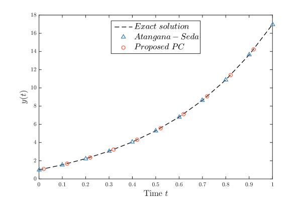
Figure 1: Solution of problem (109) for $t\in[0,1]$.

Example 2

Let us consider another initial-value problem with a classical derivative:

$$\left\{\begin{array}[]{l}\frac{dy(t)}{dt}=-\cos(2t)y^{2}(t),\text{\vskip 6.0pt plus 2.0pt minus 2.0pt}\\ y(0)=1.\end{array}\right.$$ (111)

The exact solution of this problem is known to be

$$y(t)=\frac{2}{2+\sin(2t)}.$$ (112)

The exact solution (112) is depicted in Figure 2 alongside the numerical solution obtained by means of the proposed numerical scheme (18) and the Atangana-Seda solution. The error performance is detailed in Table 2. Again, the proposed schemes achieve a noticeably superior performance.

Table 2: Comparison of the maximum absolute errors of various numerical methods for problem (111) with $t\in[0,30]$.

Method	$\Delta t=\frac{1}{16}$	$\Delta t=\frac{1}{64}$	$\Delta t=\frac{1}{200}$	$\Delta t=\frac{1}{700}$
Proposed PC (83) fractional, $\alpha=1$	$8.3152\times 10^{-3}$	$2.2772\times 10^{-5}$	$6.5114\times 10^{-7}$	$2.6151\times 10^{-8}$
Proposed PC (18)	$8.9834\times 10^{-3}$	$1.0474\times 10^{-4}$	$3.1725\times 10^{-6}$	$7.1930\times 10^{-8}$
Atangana-Seda [15]	$2.2712\times 10^{-2}$	$3.4369\times 10^{-4}$	$1.1236\times 10^{-5}$	$2.6193\times 10^{-7}$
Two-step Adams-Bashforth	$2.1387\times 10^{-2}$	$1.3589\times 10^{-3}$	$1.3984\times 10^{-4}$	$1.1436\times 10^{-5}$

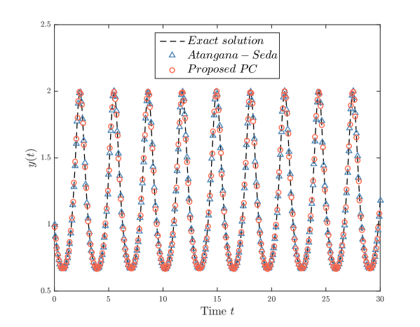
Figure 2: Solution of problem (111) for $t\in[0,30]$.

Example 3

Next, we consider the fractional Caputo initial-value problem

$$\left\{\begin{array}[]{l}\ {}_{0}^{C}D_{t}^{\alpha}y(t)=t^{\beta},\text{\vskip 6.0pt plus 2.0pt minus 2.0pt}\\ \ y(0)=0,\end{array}\right.$$ (113)

for some real constant $\beta$, which admits the unique exact solution

$$y(t)=\frac{\Gamma(\beta+1)}{\Gamma(\alpha+\beta+1)}t^{\alpha+\beta}.$$ (114)

Figure 3 shows the exact solution (114) along with the numerical solution obtained by means of the proposed predictor corrector scheme (83) and the standard and improved Atangana-Seda methods for $\beta=0.9$ and $\alpha\in\left\{0.25,0.87\right\}$. The absolute error results are presented in Table 3 for the same value of $\beta$ and $\alpha\in\left\{0.25,0.56,0.87\right\}$ with different numerical step sizes. In all scenratios, the absolute error achieved by the proposed method is lower than the improved Atangana-Seda method, which in turn is lower than the standard one.

Table 3: Comparison of the maximum absolute errors of various methods for problem (113) with $\beta=0.9$ and $t\in[0,3]$.

	$\alpha=0.25$		$\alpha=0.56$		$\alpha=0.87$
Method	$\Delta t=\frac{1}{100}$	$\Delta t=\frac{1}{800}$	$\Delta t=\frac{1}{100}$	$\Delta t=\frac{1}{400}$	$\Delta t=\frac{1}{100}$	$\Delta t=\frac{1}{200}$
PPC (83)	$6.8792\times 10^{-5}$	$6.2948\times 10^{-6}$	$2.8000\times 10^{-5}$	$3.6996\times 10^{-6}$	$7.6132\times 10^{-6}$	$4.4095\times 10^{-7}$
IAS (82)	$3.9492\times 10^{-4}$	$3.6137\times 10^{-5}$	$8.4439\times 10^{-5}$	$1.1157\times 10^{-5}$	$1.9429\times 10^{-5}$	$1.1253\times 10^{-6}$
AS [15]	$2.3016\times 10^{-3}$	$2.1060\times 10^{-4}$	$1.2783\times 10^{-3}$	$1.6891\times 10^{-4}$	$4.9855\times 10^{-4}$	$2.8876\times 10^{-5}$

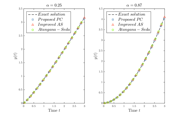
Figure 3: Solution of problem (113) for $\beta=0.9$ and $t\in[0,3]$.

Example 4

Let us consider the fractional Caputo initial-value problem

$$\left\{\begin{array}[]{l}\ {}_{0}^{C}D_{t}^{\alpha}y(t)=\frac{2t^{2-\alpha}}{\Gamma(3-\alpha)}-\frac{t^{1-\alpha}}{\Gamma(2-\alpha)}-y(t)-t+t^{2},\text{\vskip 6.0pt plus 2.0pt minus 2.0pt}\\ \ y(0)=0.\end{array}\right.$$ (115)

The exact solution of (115) can be shown to be

$$y(t)=t^{2}-t.$$ (116)

Figure 4 and Table 4 present the numerical solutions of (115) in comparison to the exact solution (116) for different fractional orders and numerical steps sizes. Again, the proposed method (83) is superior to the Atangana-Seda method and the improved method (82).

Table 4: Comparison of the maximum absolute errors of various methods for problem (115) with $t\in[0,1]$.

	$\alpha=0.4$		$\alpha=0.65$		$\alpha=0.9$
Method	$\Delta t=\frac{1}{64}$	$\Delta t=\frac{1}{512}$	$\Delta t=\frac{1}{64}$	$\Delta t=\frac{1}{512}$	$\Delta t=\frac{1}{64}$	$\Delta t=\frac{1}{512}$
PPC (83)	$7.6806\times 10^{-4}$	$6.4455\times 10^{-5}$	$3.1549\times 10^{-3}$	$4.5513\times 10^{-4}$	$6.4490\times 10^{-3}$	$8.2593\times 10^{-4}$
IAS (82)	$5.7442\times 10^{-3}$	$7.0486\times 10^{-4}$	$8.8970\times 10^{-3}$	$1.1129\times 10^{-3}$	$1.2365\times 10^{-2}$	$1.5685\times 10^{-3}$
AS [15]	$1.5787\times 10^{-2}$	$2.0038\times 10^{-3}$	$2.5879\times 10^{-2}$	$3.2837\times 10^{-3}$	$3.4087\times 10^{-2}$	$4.3577\times 10^{-3}$

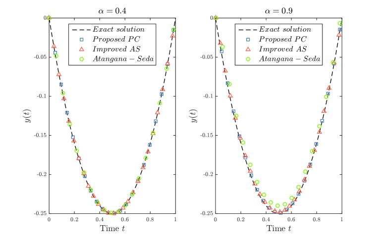
Figure 4: Solution of problem (115) for $t\in[0,1]$.

Example 5

In the previous examples, we considered some simple single differential equations with known exact solutions. Let us now analyze a realistic fractional activator-inhibitor model using analytical stability theory and validate the theoretical results numerically by means of the proposed method. Consider the system described by

$$\left\{\begin{array}[]{l}{}_{0}^{C}D_{t}^{\alpha}a(t)=\varrho_{0}\varrho+c\varrho\frac{a(t)^{2}}{h(t)}-\mu a(t),\vskip 6.0pt plus 2.0pt minus 2.0pt\\ {}_{0}^{C}D_{t}^{\alpha}h(t)=c^{\prime}\varrho^{\prime}a(t)^{2}-\nu h(t),\vskip 6.0pt plus 2.0pt minus 2.0pt\\ a(0)=a_{0},\ \ h(0)=h_{0},\end{array}\right.$$ (117)

where $a(t)$ and $h(t)$ denote the concentrations of the activator and inhibitor substances at time instant $t$, respectively. The constants $\varrho_{0}$,$\varrho$,$c$,$\mu$,$c^{\prime}$,$\varrho^{\prime}$,$a_{0}$,$h_{0}$ and $\nu$ are assumed to be positive real numbers, and the fractional differentiation order $\alpha\in(0,1]$. For $\alpha=1$, system (117) reduces to the well known Gierer-Meinhardt model describing the morphogenesis process [33, 34]. Morphogenesis is the biological process driving living organisms to take specific shapes. Inclusion of a diffusion part in the Gierer-Meinhardt model was useful in modeling the head formation of a fresh-water animal known as hydra [35]. It is well established that system (117) admits the unique equilibrium point

$$E^{\ast}=(a^{\ast},h^{\ast})$$ (118)

where

$$a^{\ast}=\frac{\varrho_{0}\varrho c^{\prime}\varrho^{\prime}+c\varrho\nu}{\mu c^{\prime}\varrho^{\prime}},$$ (119)

and

$$h^{\ast}=\frac{c^{\prime}\varrho^{\prime}}{\nu}(a^{\ast})^{2}.$$ (120)

Evaluating the Jacobian matrix of system (117) at the unique equilibrium $E^{\ast}$ yields

$$J|_{E^{\ast}}=\left(\begin{array}[]{cc}\frac{2c\mu\nu}{c\nu+c^{\prime}\varrho^{\prime}\varrho_{0}}-\mu&-\frac{c}{\varrho}\left(\frac{\mu\nu}{c\nu+c^{\prime}\varrho^{\prime}\varrho_{0}}\right)^{2}\\ \frac{2\varrho\left(c\nu+c^{\prime}\varrho^{\prime}\varrho_{0}\right)}{\mu}&-\nu\end{array}\right).$$ (121)

The determinant and trace of the Jacobian are given by

$$\mathrm{tr}J|_{E^{\ast}}=\frac{2\mu\nu c}{\nu c+\varrho_{0}\varrho^{\prime}c^{\prime}}-\mu-\nu,$$ (122)

and

$$\mathrm{det}J|_{E^{\ast}}=\mu\nu,$$ (123)

respectively. Hence, the characteristic equation of associated with $E^{\ast}$ is

$$\lambda^{2}-\lambda\mathrm{tr}J|_{E^{\ast}}+\mathrm{det}J|_{E^{\ast}}=0,$$ (124)

leading to the eigenvalues

$$\lambda_{1,2}=\frac{1}{2}\left(\mathrm{tr}J|_{E^{\ast}}\pm\sqrt{\mathrm{tr}^{2}J|_{E^{\ast}}-4\mathrm{det}J|_{E^{\ast}}}\right).$$ (125)

The dynamics of (117) can be analyzed by means of the results in [36, Section 3]. Firstly, if the discriminant of (124) is equal to zero, i.e.

$$\mathrm{tr}^{2}J|_{E^{\ast}}-4\mathrm{det}J|_{E^{\ast}}=0,$$ (126)

the eigenvelues (125) reduce to the real quantity

$$\lambda_{1,2}=\frac{1}{2}\mathrm{tr}J|_{E^{\ast}}.$$ (127)

Hence, the equilibrium $E^{\ast}$ is asymptotically stable when $\mathrm{tr}J|_{E^{\ast}}<0$ and unstable when $\mathrm{tr}J|_{E^{\ast}}>0$ for all $\alpha\in(0,1]$.

Secondly, if the discriminant is strictly positive, i.e.

$$\mathrm{tr}^{2}J|_{E^{\ast}}-4\mathrm{det}J|_{E^{\ast}}>0,$$ (128)

the eigenvalues (125) are also real. However, we distinguish two cases with respect to the asymptotic stability:

• If $\mathrm{tr}J|_{E^{\ast}}>0$, then

  $$\lambda_{1}=\frac{1}{2}\left(\mathrm{tr}J|_{E^{\ast}}+\sqrt{\mathrm{tr}^{2}J|_{E^{\ast}}-4\mathrm{det}J|_{E^{\ast}}}\right)>0.$$ (129)

  Thus, $\left|\arg(\lambda_{1})\right|=0$ and $E^{\ast}$ is unstable for all $\alpha\in(0,1]$.

• If $\mathrm{tr}J|_{E^{\ast}}<0$, then

  $$\left|\arg(\lambda_{1,2})\right|=\pi>\frac{\alpha\pi}{2}\ \text{for }\alpha\in(0,1].$$ (130)

  Thus, $E^{\ast}$ is asymptotically stable for all $\alpha\in(0,1]$.

Thirdly, if the discriminant is strictly negative, i.e.

$$\mathrm{tr}^{2}J|_{E^{\ast}}-4\mathrm{det}J|_{E^{\ast}}<0,$$ (131)

the eigenvalues become

$$\lambda_{1,2}=\frac{1}{2}\left(\mathrm{tr}J|_{E^{\ast}}\pm i\sqrt{4\mathrm{det}J|_{E^{\ast}}-\mathrm{tr}^{2}J|_{E^{\ast}}}\right),$$ (132)

leading to three distinguishable cases:

• If $\mathrm{tr}J|_{E^{\ast}}=0$, then

  $$\lambda_{1,2}=\pm i\sqrt{\mathrm{det}J|_{E^{\ast}}},$$ (133)

  leading to

  $$\left|\arg(\lambda_{1,2})\right|=\frac{\pi}{2}>\frac{\alpha\pi}{2}\text{ for }\alpha\in(0,1).$$ (134)

  Hence, $E^{\ast}$ is asymptotically stable for all $\alpha\in(0,1)$.

• If $\mathrm{tr}J|_{E^{\ast}}<0$, then

  $$\left|\arg(\lambda_{1,2})\right|>\frac{\pi}{2}>\frac{\alpha\pi}{2}\text{ for }\alpha\in(0,1),$$ (135)

  and, consequently, $E^{\ast}$ is asymptotically stable for all $\alpha\in(0,1]$.

• If $\mathrm{tr}J|_{E^{\ast}}>0$, then $E^{\ast}$ is asymptotically stable for all $\alpha\in(0,1)$ if

  $$\tan^{2}\left(\left|\mathrm{arg}\left(\lambda_{1,2}\right)\right|\right)=\frac{4\mu\nu\left(c\nu+\varrho_{0}\varrho^{\prime}c^{\prime}\right)^{2}}{\left(c\nu(\mu-\nu)-\varrho_{0}\varrho^{\prime}c^{\prime}(\mu+\nu)\right)^{2}}>\tan^{2}\left(\frac{\alpha\pi}{2}\right)+1,$$ (136)

  and unstable for all $\alpha\in(0,1)$ if

  $$\frac{4\mu\nu\left(c\nu+\varrho_{0}\varrho^{\prime}c^{\prime}\right)^{2}}{\left(c\nu(\mu-\nu)-\varrho_{0}\varrho^{\prime}c^{\prime}(\mu+\nu)\right)^{2}}<\tan^{2}\left(\frac{\alpha\pi}{2}\right)+1.$$ (137)

Remark 3

If the unique equilibrium $E^{\ast}$ of (117) is unstable for some $\alpha\in(0,1)$, then $E^{\ast}$ is also unstable for $\alpha=1$.

Since an exact solution is not available for system (117), visualizing the system dynamics requires numerical solutions, which can be obtained using the proposed predictor-corrector method described by (82)-(83). The parameters adopted for the simulations are listed in Table  5. Condition (131) can be easily verified and $\mathrm{tr}J|_{E^{\ast}}=\frac{6}{7}>0$. For $\alpha=0.85$, we have

$$\tan^{2}\left(\left|\mathrm{arg}\left(\lambda_{1,2}\right)\right|\right)=\frac{392}{9}>\tan^{2}\left(\frac{\alpha\pi}{2}\right)+1\approx 18.3497,$$ (138)

which implies that the equilibrium $E^{\ast}=(\frac{7}{4},\frac{49}{32})$ is asymptotically stable. The numerical solutions and corresponding phase plot depicted in Figures 5 and 6, respectively, agree with the theoretical analysis as the solution converges towards $(\frac{7}{4},\frac{49}{32})$. For $\alpha=0.95$, we have

$$\tan^{2}\left(\left|\mathrm{arg}\left(\lambda_{1,2}\right)\right|\right)=\frac{392}{9}<\tan^{2}\left(\frac{\alpha\pi}{2}\right)+1\approx 162.4476,$$ (139)

and thus, the equilibrium $E^{\ast}=(\frac{7}{4},\frac{49}{32})$ is unstable. Again, the numerical results shown in in Figures 7 and 8 coincide with the theoretical results as the solution is periodically stable around $(\frac{7}{4},\frac{49}{32})$. According to Remark 3, we conclude that the equilibrium $E^{\ast}$ of (117) is unstable for $\alpha=1$. This result is confirmed by the numerical results depicted in Figures 9 and 10.

Table 5: Parameter values of system (117) adopted in the numerical simulations.

$\varrho_{0}$	$\varrho$	$\mu$	$\nu$	$c$	$\varrho^{\prime}$	$c^{\prime}$	$a_{0}$	$h_{0}$
$1$	$1$	$4$	$2$	$3$	$1$	$1$	$2$	$3$

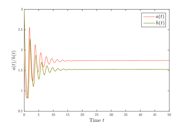
Figure 5: The numerical solution of system (117) for $\alpha=0.85$ with the parameters listed in Table 5.

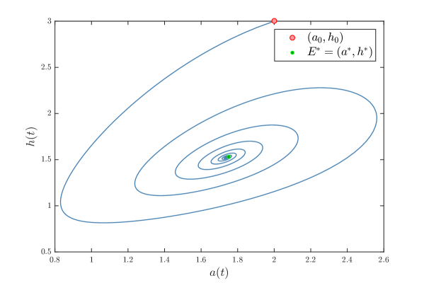
Figure 6: Phase plot of system (117) for $\alpha=0.85$ with the parameters listed in Table 5.

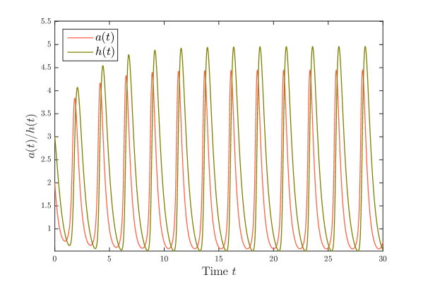
Figure 7: The numerical solution of system (117) for $\alpha=0.95$ with the parameters listed in Table 5.

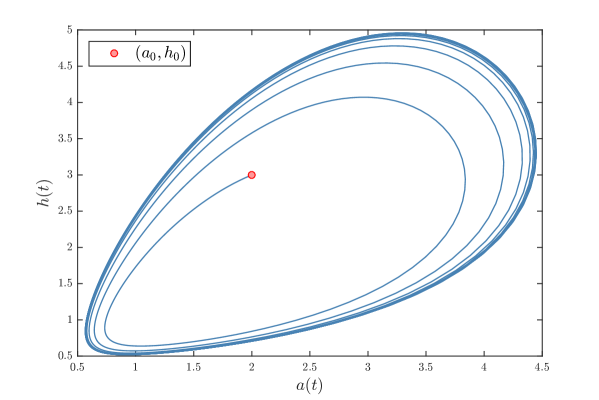
Figure 8: Phase plot of system (117) for $\alpha=0.95$ with the parameters listed in Table 5.

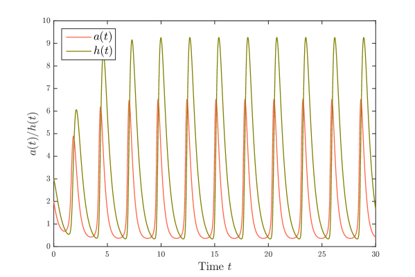
Figure 9: The numerical solution of system (117) for $\alpha=1$ with the parameters listed in Table 5.

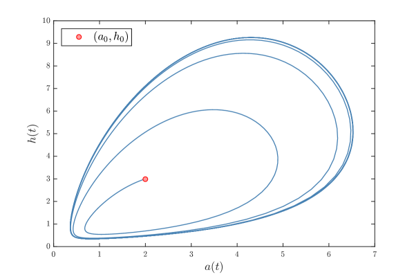
Figure 10: Phase plot of system (117) for $\alpha=1$ with the parameters listed in Table 5.

5 Conclusion

In this paper, we have employed one/two steps first/second order Newton polynomial interpolation to derive new two methods to solve fractional differential equations for several definitions of the fractional derivative, the first one method is the improved version of the Atangana-Seda method which has been widely used in a short time period since its appearance, and the second one method we have proposed new predictor-corrector method and we have used improved Atangana-Seda scheme as a predictor term. The proposed methods have demonstrated their effectiveness with the various examples presented and have proven effective for obtaining accurate approximate solutions for complex systems. The simplicity of displaying proposed methods equations enables us to easily convert them into algorithms and translate them into different programming languages for use in numerical simulations of systems modeling various phenomena in the real world. These methods will open new horizons in the field of numerical analysis of fractional differential equations with many definitions of fractional derivative.

References

References

- [1] W. Werner, Polynomial interpolation: Lagrange versus Newton, Math. Comput., Vol. 43 (1984), pp. 205-217.
- [2] T. Fred, W. Krogh, Efficient algorithms for polynomial interpolation and numerical differentiation, Math. Comput., Vol. 24 (1970), pp. 185-190.
- [3] Y. Yang, S. P. Gordon, Visualizing and understanding the components of Lagrange and Newton interpolation, Probl. Resour. Issues Math. Undergrad. Stud., Vol. 26(1) (2015), pp. 39-52.
- [4] D. K. Dimitrov, G. M. Philipps, A note on convergence of Newton interpolating polynomials, J. Comput. Appl. Math., Vol. 51(1) (1994), pp. 127-130.
- [5] K. Diethelm, A. D. Freed, The FracPECE subroutine for the numerical solution of differential equations of fractional order, Forschung und wissenschaftliches Rechnen, Vol. 1999 (1998), pp. 57-71.
- [6] N. J. Ford, A. C. Simpson, The numerical solution of fractional differential equations: speed versus accuracy, Numerical Algorithms, Vol. 26(4) (2001), pp. 333-346.
- [7] Z. Odibat, S. Momani, An algorithm for the numerical solution of differential equations of fractional order, J. Appl. Math. Inform, Vol. 26(1-2) (2008), pp. 15-27.
- [8] B. P. Moghaddam, S. Yaghoobi, J. A. T. Machado, An extended predictor-corrector algorithm for variable-order fractional delay differential equations, J. Computational and Nonlinear Dynamics, Vol. 11(6) (2016).
- [9] M. S. Asl, M. Javidi, An improved PC scheme for nonlinear fractional differential equations: Error and stability analysis, J. Comput. Appl. Math., Vol. 324 (2017), pp. 101-117.
- [10] M. F. S. Patricio, H. Ramos, M. Patricio, Solving initial and boundary value problems of fractional ordinary differential equations by using collocation and fractional powers, J. Comput. Appl. Math., Vol. 354 (2019), pp. 348-359.
- [11] T. Zhang, J. Jin, T. Jiang, The decoupled Crank-Nicolson/Adams-Bashforth scheme for the Boussinesq equations with nonsmooth initial data, Appl. Math. Comput., Vol. 337 (2018), pp. 234-266.
- [12] S. Jain, Numerical analysis for the fractional diffusion and fractional buckmaster equation by the two-step Laplace Adam-Bashforth method, Eur. Phys. J. Plus, Vol. 133(1) (2018), pp. 1-11.
- [13] R. B. Srivastava, S. Shukla, Numerical Accuracies of Lagrange’s and Newton Polynomial Interpolation: Numerical Accuracies of Interpolation Formulas, LAP LAMBERT Academic Publishing, 2012.
- [14] R. B. Srivastava, P. K. Srivastava, Comparison of Largrange’s and Newton’s interpolating polynomials, J. Experimental Sciences, Vol. 3(1) (2012), pp. 01-04.
- [15] A. Atangana, I. A. Seda, New numerical method for ordinary differential equations: Newton polynomial, J. Comput. Appl. Math., Vol. 372 (2020), 112622.
- [16] A. Atangana, I. A. Seda, Corrigendum to New numerical method for ordinary differential equations: Newton polynomial[J. Comput. Appl. Math. (2019) 112622], J. Comput. Appl. Math., Vol. 371 (2020), 112668.
- [17] B. S. T. Alkahtani, A new numerical scheme based on Newton polynomial with application to fractional nonlinear differential equations, Alexandria Engineering Journal, DOI: https://doi.org/10.1016/j.aej.2019.11.008
- [18] A. Atangana, S. Igret Araz, New numerical approximation for Chua attractor with fractional and fractal-fractional operators, Alexandria Engineering Journal, DOI: https://doi.org/10.1016/j.aej.2020.01.004
- [19] A. Atangana, S. Igret. Araz, Atangana-Seda numerical scheme for Labyrinth attractor with new differential and integral operators, Fractals, DOI: https://doi.org/10.1142/S0218348X20400447
- [20] A. Atangana, S. Igret. Araz, Extension of Atangana-Seda numerical method to partial differential equations with integer and non-integer order, Alexandria Engineering Journal, DOI: https://doi.org/10.1016/j.aej.2020.02.031
- [21] W.B. Gragg, H.J. Stetter, Generalized multistep predictor-corrector methods, J. Association for Computing Machinery, Vol. 11(2) (1964), pp. 188-209.
- [22] A. Marciniak, M. A. Jankowska, T. Hoffmann, On interval predictor-corrector methods, Numerical Algorithms, Vol. 75 (2017), pp. 777-808.
- [23] J.C. Butcher, Numerical methods for ordinary differential equations, 3rd editor, John Wiley and Sons Ltd., 2016.
- [24] K. Diethelm, N. J. Ford, A. D. Freed, A predictor-corrector approach for the numerical solution of fractional differential equations, Nonlinear Dynamics, Vol. 29 (2002), pp. 3-22.
- [25] T. B. Nguyen, B.Jang, A high-order predictor-corrector method for solving nonlinear differential equations of fractional order, Fractional Calculus and Applied Analysis, Vol. 20(2) (2017), pp. 447–476.
- [26] R. Douaifia, S. Abdelmalek, A predictor-corrector method for fractional delay-differential system with multiple lags, Communications in Nonlinear Analysis, Vol. 6(1) (2019), pp. 78-88.
- [27] M. Kumar, V. Daftardar-Gejji, A new family of predictor-corrector methods for solving fractional differential equations, Applied Mathematics and Computation, Vol. 363 (2019), 124633.
- [28] M. S. Heris, M. Javidi, A predictor-corrector scheme for the tempered fractional differential equations with uniform and non-uniform meshes, J. Supercomputing, Vol. 12 (2019).
- [29] I. Podlubny, Fractional differential equations. New York: Academic Press; 1999.
- [30] A. A. Kilbas, H. M. Srivastava, J. J. Trujillo, Theory and applications of fractional differential equations (Vol. 204). elsevier; 2006.
- [31] M. Caputo, M. Fabrizio, A new definition of fractional derivative without singular kernel, Progr. Fract. Differ. Appl, Vol. 1(2) (2015), pp. 1-13.
- [32] A. Atangana, D. Baleanu, New fractional derivative with non-local and non-singular kernel, Therm. Sci., Vol. 20 (2016), pp. 757-763.
- [33] M. I. Granero-Porati, A. Porati, Temporal organization in a morphogenetic field, Journal of Mathematical Biology, Vol. 20(2) (1984), pp. 153-157.
- [34] S. Ruan, Diffusion-driven instability in the Gierer-Meinhardt model of morphogenesis, Natural Resource Modeling, Vol. 11(2) (1998), pp. 131-141.
- [35] A. Gierer, H. Meinhardt, A theory of biological pattern formation, Kybernetik, Vol. 12(1) (1972), pp. 30-39.
- [36] E. Ahmed, A. M. A. El-Sayed, H. A. A. El-Saka, Equilibrium points, stability and numerical solutions of fractional-order predator-prey and rabies models, Journal of Mathematical Analysis and Applications, Vol. 325(1) (2007), pp. 542-553.