Highly nonclassical phonon emission statistics through two-phonon loss of van der Pol oscillator

Abstract

The ability to produce nonclassical wave in a system is essential for advances in quantum communication and computation. Here, we propose a scheme to generate highly nonclassical phonon emission statistics—antibunched wave in a quantum van der Pol (vdP) oscillator subject to an external driving, both single- and two-phonon losses. It is found that phonon antibunching depends significantly on the nonlinear two-phonon loss of the vdP oscillator, where the degree of the antibunching increases monotonically with the two-phonon loss and the distinguished parameter regimes with optimal antibunching and single-phonon emission are identified clearly. In addition, we give an in-depth insight into strong antibunching in the emitted phonon statistics by analytical calculations using a three-oscillator-level model, which agree well with the full numerical simulations employing both a master-equation approach and a Schrödinger-equation approach at weak driving. In turn, the fluorescence phonon emission spectra of the vdP oscillator, given by the power spectral density, are also evaluated. We further show that high phonon emission amplitudes, simultaneously accompanied by strong phonon antibunching, are attainable in the vdP system, which are beneficial to the correlation measurement in practical experiments. Our approach only requires a single vdP oscillator, without the need for reconfiguring the two coupled nonlinear resonators or the complex nanophononic structures as compared to the previous blockade schemes. The present scheme could inspire methods to achieve antibunching in other systems.

I Introduction

In analogy to the photon antibunching I-1 ; I-2 ; I-3 ; I-4 ; I-5 ; I-6 ; I-7 ; I-8 ; I-9 ; I-10 ; I-11 ; I-12 , the phonon antibunching refers to the phenomenon that the coupling of a single phonon to the system hinders the coupling of the subsequent phonons, which is a pure nonclassical effect owing to less than unity value of the normalized second-order correlation function of the phonon field. The phonon antibunching is important in uncovering the quantum behaviors of the mechanical vibration and in realizing a single-phonon source and other single-phonon quantum devices. Here, on the one hand, the phonons are produced by a mechanical vibration (a motional degree of freedom) and are the outcome of the vibration quantization I-13a ; I-13b . Generally, the mechanical vibration frequencies are typically on the order of MHz and GHz, which is quite different from the ones of the photons. On the other hand, the phonons, like the photons, belong to the bosons and belong to the category of quantum harmonic oscillators. Moreover, their mechanical operators have the same correspondence. As a result, the signatures of the phonon antibunching (also called as phonon blockade) can be detected through the phonon-statistics measurements, such as the above-mentioned second-order correlation function at zero time delay I-14 ; I-15 . The realization of the phonon antibunching generally needs a large quantum mechanical nonlinearity like the photon antibunching. In recent years, it has been shown that this mechanical nonlinearity can be achieved in hybrid systems with the mechanical oscillator coupled to a single qubit fa1 ; fa2 ; fa3 ; fa4 and in optomechanical systems with quadratic or three-mode coupling fb1 ; fb2 . Single-photon-induced phonon blockade has been investigated theoretically in a hybrid spin-optomechanical system I-16 .

On the other hand, the mechanical van der Pol (vdP) oscillator is very extensive in natural and engineered systems. Since the prototypical model of the mechanical vdP oscillator was first proposed by Balthazar van der Pol fc1 in 1926, it has attracted considerable attention in the classical level. In the past few years, this vdP model has been successfully extended from a classical regime to a full quantum regime, i.e., the so-called quantum vdP oscillator, and also has drawn a great deal of research interests in the quantum level. The particles in the vdP field are usually called the phonons based on the literatures VI-1 ; VI-2 ; VI-3 ; VI-4 ; VI-5 ; VI-6 ; VI-7 ; V-8 ; V-9 ; I-79 ; I-80 ; I-81 ; I-82 and the system is also called a phonon vdP oscillator. We notice that the previous works shed light on the quantum synchronization, limit-cycle, frequency entrainment, and diverging and negative susceptibilities of a quantum vdP oscillator VI-1 ; VI-2 ; VI-3 ; VI-4 ; VI-5 ; VI-6 ; VI-7 ; V-8 ; V-9 or the entanglement tongue and quantum synchronization of two coupled quantum vdP oscillators I-79 ; I-80 ; I-81 , differing from what are found in the classical regime. The multiple resonances of the mean phonon number are demonstrate in two coupled quantum anharmonic vdP oscillators and the genuine quantum effects are also expected in the amplitude death phenomenon I-82 . To date, there seems to exist no works in the literature dealing with the above-mentioned nonclassical phonon antibunching in a quantum vdP oscillator. Is there strong antibunching effect? How does quantum noise (the dissipative coupling) effect the antibunching?

Motivated by these facts and to answer these issues above, in the present work we theoretically investigate the characteristics of antibunched phonons generated in a driven quantum vdP oscillator with both single- and two-phonon losses. By means of the second-order correlation function $g^{(2)}(0)$ providing information on phonon bunching and antibunching, we show that the degree of phonon antibunching is governed sensitively by the nonlinear two-phonon loss of the vdP oscillator. Increasing the two-phonon loss increases the degree of the phonon antibunching with experimentally achievable parameters. This occurs because a large two-phonon loss decouples the third level of an oscillator leaving an effective driven two-level system. We identify clearly distinguished parameter regimes with strong antibunching and single-phonon emission. On the other hand, we present analytical solutions of the second-order correlation function based on a three-oscillator-level approximation, which match the full numerical simulations based on a quantum master equation and a Schrödinger equation at weak driving. Additionally, we analyze the fluorescence phonon emission spectra of the vdP oscillator by properly varying the two-phonon loss. It is found that high phonon emission amplitudes, accompanied by strong phonon antibunching (single-phonon emission), can be achieved efficiently. This result is useful for the correlation measurement in practical experiments.

Compared with the previous phonon antibunching or blockade schemes fa1 ; fa2 ; fa3 ; fa4 ; fb1 ; fb2 , our approach is based entirely on a single vdP oscillator, eliminating the need for coupled nonlinear resonators or complex nanophononic structures. On the other hand, our achievable antibunching effect, $g^{(2)}(0)<1$, can occur, without requiring fine trade-off and tuning between the loss rate and the nonlinearity. In particular, the degree of phonon antibunching can be kept high even for the case that the nonlinear two-phonon damping is less than the linear single-phonon damping. Finally, we briefly discuss specific implementations based respectively on an ion trap VI-1 ; VI-2 ; VI-3 ; VI-4 ; VI-5 ; VI-6 ; VI-7 and an optomechanical membrane VI-8 ; VI-9 ; VI-10 . Our study contributes insights in understanding phonon-phonon correlation in the quantum vdP field.

Finally, it is worth pointing out that the same model in the presence of both the photon-photon (or phonon-phonon) interaction and the two-photon (or two-phonon) driving has been proposed and explored by means of the complex P-representation formalism by Bartolo et. al r1 . Many interesting features, including controllable Wigner-function multimodality, dissipative phase transitions, quantum trajectories, and Schrödinger cat states, have been elaborated in the Bartolo’s model or approximate model r1 ; r2 ; r3 . But, these are very different scenarios to ours as we are interested in quantum statistics of the phonon emitted in the vdP oscillator in the absence of the phonon-phonon interaction and the two-phonon driving, namely, such a regime is not addressed explicitly in the works mentioned before. From an experimental point of view, this is beneficial because there is no need for invoking the additional Kerr nonlinearity and parametrical driving source, which makes the implementation of this proposal more experimental friendly.

This paper is organized as follows. In Sec. II, we describe the quantum model of a driven vdP oscillator under consideration and yield the Lindblad master equation which governs the dissipative dynamics of the vdP oscillator. In Sec. III, we introduce the second-order intensity correlation function which provides information on the degree of phonon bunching and antibunching. Subsequently, in Sec. IV, we provide analytical insights into the second-order correlation function based on a three-oscillator-level model (Sec. IV.1) via a master equation approach and further find approximate solutions of the second-order correlation function (Sec. IV.2). Again, starting from a Schrödinger equation approach, an analytical discussion for the second-order correlation function of the system is presented (Sec. IV.3). This three-oscillator-level model is a justifiable approximation for low driving strengths. In Sec. V, we explore in details phonon correlation characteristics without and with time delay, as well as emission spectrum of the vdP oscillator by adjusting the typical parameters, especially dissipative engineering the two-phonon loss. In Sec. VI, we elaborate on an ion trap and optomechanical implementations of the quantum vdP oscillator. Finally, we summarize our results in Sec. VII.

II System of a quantum vdP oscillator: Hamiltonian and master equation treatment

We first introduce our model of the system. We consider a quantum vdP oscillator of interest, subject to an external continuous-wave driving of strength $E_{d}$ and frequency $\omega_{d}$, i.e., $S_{dri}(t)=E_{d}e^{-i\omega_{d}t}$. Our oscillator model involves two dissipation processes, one being a linear single-phonon loss of rate $\kappa_{1}$ and the other being a nonlinear two-phonon loss of rate $\kappa_{2}$, as in Refs. VI-1 ; VI-2 ; VI-3 ; VI-4 ; VI-5 ; VI-6 ; VI-7 . Nevertheless, our model makes a slight adjustment of the usual quantum vdP oscillator, where the single-phonon gain is replaced with the single-phonon loss since the presence of the single-phonon loss is preferred to obtain strong phonon antibunching, and, on the other hand, it is much easier to achieve experimentally. Such dissipation processes can be engineered in current experimental platforms by coupling the oscillator to a suitable environment, as will be discussed later. The Hamiltonian and the Lindblad master equation for this model, in the frame rotating at the frequency $\omega_{d}$ of the external driving, read (setting $\hbar=1$ throughout this work)

$$\hat{H}_{osc} = \hat{H}_{0}+\hat{H}_{dri}=\Delta\hat{a}^{{\dagger}}\hat{a}+iE_{d}(\hat{a}-\hat{a}^{{\dagger}}),$$ (1)

$$\frac{d\hat{\rho}}{dt} = -i[\hat{H}_{osc},\hat{\rho}]+\frac{1}{2}\kappa_{1}\mathcal{D}(\hat{a})\hat{\rho}+\frac{1}{2}\kappa_{2}\mathcal{D}(\hat{a}^{2})\hat{\rho},$$ (2)

where $\hat{a}$ ($\hat{a}^{{\dagger}}$) is the oscillator annihilation (creation) operator satisfying bosonic commutation relation $[\hat{a},\hat{a}^{{\dagger}}]=1$, $\Delta=\omega_{a}-\omega_{d}$ is the detuning between the vdP oscillator frequency $\omega_{a}$ and the external driving frequency $\omega_{d}$, and $\hat{\rho}$ is the density matrix operator, respectively. Applying the unitary transformation $\hat{U}=\exp(i\omega_{d}\hat{a}^{{\dagger}}\hat{a}t)$ leads to Eq. (1) above: $\hat{H}_{osc}=\hat{U}\hat{H}_{old}\hat{U}^{{\dagger}}-i\hat{U}\partial\hat{U}^{{\dagger}}/\partial t$, where $\hat{H}_{old}=\omega_{a}\hat{a}^{{\dagger}}\hat{a}+iE_{d}(e^{i\omega_{d}t}\hat{a}-e^{-i\omega_{d}t}\hat{a}^{{\dagger}})$, under the helps of $\hat{U}\hat{a}\hat{U}^{{\dagger}}=\hat{a}e^{-i\omega_{d}t}$, $\hat{U}\hat{a}^{{\dagger}}\hat{U}^{{\dagger}}=\hat{a}^{{\dagger}}e^{i\omega_{d}t}$, and $\hat{U}\partial\hat{U}^{{\dagger}}/\partial t=-i\omega_{d}\hat{a}^{{\dagger}}\hat{a}$. In the driving term $\hat{H}_{dri}=iE_{d}(\hat{a}-\hat{a}^{{\dagger}})$ in Eq. (1), the rotating-wave approximation has been applied; without the loss of generality, we set $E_{d}$ to be real. $\hat{H}_{0}=\Delta\hat{a}^{{\dagger}}\hat{a}$ is the unperturbed Hamiltonian of the oscillator relative to $\omega_{d}$. Above, in Eq. (2) we have introduced the Lindblad operator $\mathcal{D}(\hat{\mathcal{O}})\hat{\rho}=2\hat{\mathcal{O}}\hat{\rho}\hat{\mathcal{O}}^{{\dagger}}-\hat{\rho}\hat{\mathcal{O}}^{{\dagger}}\hat{\mathcal{O}}-\hat{\mathcal{O}}^{{\dagger}}\hat{\mathcal{O}}\hat{\rho}$ to describe the nonunitary dynamics with $\hat{\mathcal{O}}$ being the relevant operators $\hat{a}$ and $\hat{a}^{2}$. This master equation can be used to derive the steady state for the following second-order correlation function.

III Second-order correlation function providing information on phonon (anti)bunching

The appeal of the quantum vdP oscillator is that owing to its simple form, it can serve as a prototypical model for studying its nonclassical properties in the quantum limit. Here we concentrate on the phonon statistics of the quantum vdP oscillator. To this end, our central task in this work is to calculate the normalized second-order correlation function $g^{(2)}(\tau)$, which is defined, for the phonon vdP oscillator in the steady state, as V-5 ; V-6 ; V-7 ; V-10

$$g^{(2)}(\tau) = \frac{\mbox{Tr}[\hat{\rho}\hat{a}^{{\dagger}}(0)\hat{a}^{{\dagger}}(\tau)\hat{a}(\tau)\hat{a}(0)]}{\{\mbox{Tr}[\hat{\rho}\hat{a}^{{\dagger}}(0)\hat{a}(0)]\}^{2}}$$ (3)

$$= \frac{\langle\hat{a}^{{\dagger}}(0)\hat{a}^{{\dagger}}(\tau)\hat{a}(\tau)\hat{a}(0)\rangle}{\langle\hat{a}^{{\dagger}}(0)\hat{a}(0)\rangle^{2}},$$

where $\langle\hat{\mathcal{O}}\rangle=\mbox{Tr}(\hat{\rho}\hat{\mathcal{O}})$ denotes the expectation values taken with respect to the steady-state density matrix of the full Lindblad master equation (2), and $\tau$ is the time between the arrival of the first and second phonons, i.e., time delay. $g^{(2)}(\tau)$ can be understood as the conditional probability of detecting a phonon at time $\tau$ provided that one phonon was detected earlier at time $\tau=0$. It can be proved that the second-order correlation function $g^{(2)}(\tau)$ satisfies the properties of, on the one hand, time symmetry $g^{(2)}(-\tau)=g^{(2)}(\tau)$, and, on the other hand, non-negativity $g^{(2)}(\tau)\geq 0$.

If $\tau=0$, we refer to $g^{(2)}(0)$ as a zero-time-delay second-order correlation function. For the case of zero time delay, it is known that the value of $g^{(2)}(0)<1$ [$g^{(2)}(0)>1$] corresponds to sub-Poissonian (super-Poissonian) statistics of the vdP oscillator field, which is a nonclassical antibunching (classical bunching) effect. Alternatively, $g^{(2)}(0)=1$ represents a coherent light source.

One can numerically calculate the steady-state solution of the master equation Eq. (2) with the left-hand side set to zero, from which the steady-state second-order correlation function $g^{(2)}(\tau)$ is obtained. For this purpose, we truncate the vdP field’s Hilbert space sufficiently large, for example, at phonon numbers as large as $100$ for the vdP oscillator mode to ensure full convergence. Finally, all calculations are performed in the frame rotating with the driving frequency $\omega_{d}$.

IV Two-type analytical insights into the second-order correlation function by a three-oscillator-level approximation

IV.1 Three-oscillator-level approximation via a master equation approach

Before proceeding, we develop a three-oscillator-level model that provides further physical insight into the numerical results. For this purpose, in the Hilbert space of Fock states $\{|n\rangle\}$ with $n=0,1,2,\ldots$ being the number of phonons in the oscillator mode, the Lindblad master equation (2) can be written as

$$\frac{d\rho_{n,m}}{dt} = -i\Delta\left(n-m\right)\rho_{n,m}$$ (4)

$$+ E_{d}\left(\sqrt{n+1}\rho_{n+1,m}-\sqrt{n}\rho_{n-1,m}\right)$$

$$+ E_{d}\left(\sqrt{m+1}\rho_{n,m+1}-\sqrt{m}\rho_{n,m-1}\right)$$

$$+ \kappa_{1}\left[\sqrt{(n+1)(m+1)}\rho_{n+1,m+1}-\frac{n+m}{2}\rho_{n,m}\right]$$

$$+ \kappa_{2}\left[\sqrt{(n+1)(n+2)}\sqrt{(m+1)(m+2)}\rho_{n+2,m+2}\right.$$

$$- \left.\frac{n(n-1)+m(m-1)}{2}\rho_{n,m}\right],$$

where $\rho_{n,m}=\langle n|\hat{\rho}|m\rangle=\langle m|\hat{\rho}|n\rangle^{*}$ is the matrix element of the density operator $\hat{\rho}$. The diagonal element $\rho_{n,n}$ denotes the occupying probability in the state $|n\rangle$, whereas the off-diagonal element $\rho_{n,m}$ ($n\neq m$) represents the coherence between the states $|n\rangle$ and $|m\rangle$.

Next, we approximate the oscillator modes by retaining the lowest three oscillator levels, $n=0,1,2$, in Eq. (4). In this scenario, we have the equations of motion for the density operator matrix element $\rho_{n,m}$ as follows:

$$\frac{d\rho_{1,1}}{dt} = -\kappa_{1}\rho_{1,1}+2\kappa_{1}\rho_{2,2}+\sqrt{2}E_{d}\rho_{2,1}+\sqrt{2}E_{d}\rho_{1,2}$$ (5)

$$-E_{d}\rho_{0,1}-E_{d}\rho_{1,0},$$

$$\frac{d\rho_{2,2}}{dt} = -2(\kappa_{1}+\kappa_{2})\rho_{2,2}-\sqrt{2}E_{d}\rho_{2,1}-\sqrt{2}E_{d}\rho_{1,2},$$ (6)

$$\frac{d\rho_{1,0}}{dt} = -\left(i\Delta+\frac{1}{2}\kappa_{1}\right)\rho_{1,0}+2E_{d}\rho_{1,1}+E_{d}\rho_{2,2}$$ (7)

$$+\sqrt{2}\kappa_{1}\rho_{2,1}+\sqrt{2}E_{d}\rho_{2,0}-E_{d},$$

$$\frac{d\rho_{2,1}}{dt} = -\left(i\Delta+\frac{3}{2}\kappa_{1}+\kappa_{2}\right)\rho_{2,1}+\sqrt{2}E_{d}\left(\rho_{2,2}-\rho_{1,1}\right)$$ (8)

$$-E_{d}\rho_{2,0},$$

$$\frac{d\rho_{2,0}}{dt} = -\left(2i\Delta+\kappa_{1}+\kappa_{2}\right)\rho_{2,0}+E_{d}\rho_{2,1}$$ (9)

$$-\sqrt{2}E_{d}\rho_{1,0},$$

where $\rho_{0,0}=1-\rho_{1,1}-\rho_{2,2}$.

In the steady state limit, i.e, setting $d\rho_{n,m}/dt=0$ in the left-hand side of Eqs. (5)-(9), we have the results

$$-\kappa_{1}\rho_{1,1}+2\kappa_{1}\rho_{2,2}+\sqrt{2}E_{d}\rho_{2,1}+\sqrt{2}E_{d}\rho_{1,2}-E_{d}\rho_{0,1}$$

$$-E_{d}\rho_{1,0}=0,$$ (10)

$$-2(\kappa_{1}+\kappa_{2})\rho_{2,2}-\sqrt{2}E_{d}\rho_{2,1}-\sqrt{2}E_{d}\rho_{1,2}=0,$$ (11)

$$-\left(i\Delta+\frac{1}{2}\kappa_{1}\right)\rho_{1,0}+2E_{d}\rho_{1,1}+E_{d}\rho_{2,2}+\sqrt{2}\kappa_{1}\rho_{2,1}$$

$$+\sqrt{2}E_{d}\rho_{2,0}=E_{d},$$ (12)

$$-\left(i\Delta+\frac{3}{2}\kappa_{1}+\kappa_{2}\right)\rho_{2,1}+\sqrt{2}E_{d}\left(\rho_{2,2}-\rho_{1,1}\right)$$

$$-E_{d}\rho_{2,0}=0,$$ (13)

$$-\left(2i\Delta+\kappa_{1}+\kappa_{2}\right)\rho_{2,0}+E_{d}\rho_{2,1}-\sqrt{2}E_{d}\rho_{1,0}=0.$$ (14)

This set of equations (10)-(14) together with the corresponding complex conjugations can be solved by first expressing in the matrix form,

$$\mathbf{M}\mathbf{R}=\mathbf{V},$$ (15)

where the elements of the matrices are respectively presented by $\mathbf{R}=(\rho_{1,1},\rho_{2,2},\rho_{1,0},\rho_{0,1},\rho_{2,1},\rho_{1,2},\rho_{2,0},\rho_{0,2})^{T}$, $\mathbf{V}=(0,0,E_{d},E_{d},0,0,0,0)^{T}$, and

$$\mathbf{M}=\left(\begin{array}[]{cccccccc}-\kappa_{1}&2\kappa_{2}&-E_{d}&-E_{d}&\sqrt{2}E_{d}&\sqrt{2}E_{d}&0&0\\ 0&-2(\kappa_{1}+\kappa_{2})&0&0&-\sqrt{2}E_{d}&-\sqrt{2}E_{d}&0&0\\ 2E_{d}&E_{d}&-i\Delta-\frac{1}{2}\kappa_{1}&0&\sqrt{2}\kappa_{1}&0&\sqrt{2}E_{d}&0\\ 2E_{d}&E_{d}&0&i\Delta-\frac{1}{2}\kappa_{1}&0&\sqrt{2}\kappa_{1}&0&\sqrt{2}E_{d}\\ -\sqrt{2}E_{d}&\sqrt{2}E_{d}&0&0&-i\Delta-\frac{3}{2}\kappa_{1}-\kappa_{2}&0&-E_{d}&0\\ -\sqrt{2}E_{d}&\sqrt{2}E_{d}&0&0&0&i\Delta-\frac{3}{2}\kappa_{1}-\kappa_{2}&0&-E_{d}\\ 0&0&-\sqrt{2}E_{d}&0&E_{d}&0&-2i\Delta-\kappa_{1}-\kappa_{2}&0\\ 0&0&0&-\sqrt{2}E_{d}&0&E_{d}&0&2i\Delta-\kappa_{1}-\kappa_{2}\\ \end{array}\right).$$ (24)

The solutions of $\mathbf{R}$ are given by $\mathbf{R}=\mathbf{M}^{-1}\mathbf{V}$ with $\mathbf{M}^{-1}$ denoting the inverse matrix of $\mathbf{M}$, and here $\mathbf{M}^{-1}$ is too lengthy and uninspiring to be displayed. In order to capture the main physics, we consider some particular cases of interest and derive closed-form expressions of $\mathbf{R}$. First, the driving is set on resonance with the vdP oscillator, i.e., $\Delta=0$ for simplicity. Second, the condition of weak external driving holds, i.e., $E_{d}\ll\kappa_{1},\kappa_{2}$, in order to guarantee the validity of the three-level model. With these assumptions discussed above, $\rho_{1,1}$ and $\rho_{2,2}$ we need in the solutions of $\mathbf{R}$ [see Eq. (29) later for clarity], to the quartic order in the variables $E_{d}/\kappa_{1}$ and $E_{d}/\kappa_{2}$ after tedious calculations, are

$$\rho_{1,1} = \left[2+\frac{\kappa_{1}^{2}}{4E_{d}^{2}}+\frac{2\kappa_{1}\kappa_{2}-2\kappa_{1}^{2}}{(\kappa_{1}+\kappa_{2})(3\kappa_{1}+2\kappa_{2})}-\frac{4\kappa_{1}}{3\kappa_{1}+2\kappa_{2}}+\frac{\kappa_{1}}{\kappa_{1}+\kappa_{2}}+\frac{8\kappa_{2}E_{d}^{2}}{(\kappa_{1}+\kappa_{2})^{2}(3\kappa_{1}+2\kappa_{2})}\right]^{-1},$$ (25)

$$\rho_{2,2} = \left[\frac{4E_{d}^{2}}{(\kappa_{1}+\kappa_{2})(3\kappa_{1}+2\kappa_{2})}+\frac{2\kappa_{1}E_{d}^{2}}{(\kappa_{1}+\kappa_{2})^{2}(3\kappa_{1}+2\kappa_{2})}\right]\rho_{1,1}.$$ (26)

IV.2 Analytical expressions for the second-order correlation function

According to $\hat{a}^{{\dagger}}\hat{a}|n\rangle=n|n\rangle$ and $\hat{a}^{{\dagger}2}\hat{a}^{2}|n\rangle=n(n-1)|n\rangle$, we have $\langle n|\hat{\rho}\hat{a}^{{\dagger}}\hat{a}|n\rangle=n\rho_{n,n}$ and $\langle n|\hat{\rho}\hat{a}^{{\dagger}2}\hat{a}^{2}|n\rangle=n(n-1)\rho_{n,n}$. So, the zero-time-delay second-order correlation function $g^{(2)}(0)$ can be recast in the form

$$g^{(2)}(0) = \frac{\sum\limits_{n}n(n-1)\rho_{n,n}}{\left(\sum\limits_{n}n\rho_{n,n}\right)^{2}}$$ (27)

$$= \frac{2\rho_{2,2}+6\rho_{3,3}+\cdots}{(\rho_{1,1}+2\rho_{2,2}+\cdots)^{2}},$$

where the sum index $n=0,1,2,\cdots$. Obviously, nonclassical antibunching (sub-Poissonian statistics) requires that the numerator of Eq. (27) is smaller than its denominator. For example, this can be achieved either by maximizing $\rho_{1,1}$ or decreasing $\rho_{2,2}$. Note that, the component of $n=0$ need not be considered owing to the vanishing value.

Under the weak driving condition where $\rho_{n,n}$ vanishes quickly with $n$, we have the relationship

$$\rho_{0,0}\gg\rho_{1,1}\gg\rho_{2,2}\gg\rho_{3,3}\gg\cdots.$$ (28)

In view of this, by the truncation, the $g^{(2)}(0)$ function from Eq. (27) can be approximately reduced into the simple expression

$$g^{(2)}(0)\simeq\frac{2\rho_{2,2}}{\rho_{1,1}^{2}},$$ (29)

or

$$g^{(2)}(0) \simeq \left[\frac{8E_{d}^{2}}{(\kappa_{1}+\kappa_{2})(3\kappa_{1}+2\kappa_{2})}\right.$$ (30)

$$\left.+\frac{4\kappa_{1}E_{d}^{2}}{(\kappa_{1}+\kappa_{2})^{2}(3\kappa_{1}+2\kappa_{2})}\right]\times\frac{1}{\rho_{1,1}},$$

where the two desired matrix elements $\rho_{2,2}$ and $\rho_{1,1}$ are yielded by Eqs. (25) and (26).

As an aside, we note that when the two-phonon loss is much stronger than the single-phonon loss ($\kappa_{2}\gg\kappa_{1}$), retaining the lowest order in $E_{d}/\kappa_{1}$, $E_{d}/\kappa_{2}$ and $\kappa_{1}/\kappa_{2}$, the $g^{(2)}(0)$ function from Eq. (30) can be further reduced into a compact form

$$g^{(2)}(0)\simeq\left(\frac{\kappa_{1}}{\kappa_{2}}\right)^{2}\sim 0,$$ (31)

which coincides with the numerical simulation based on the full quantum master equation (2) in the aforementioned parameter range, as can be found in Fig. 1 below.

IV.3 Three-oscillator-level approximation via a Schrödinger equation approach

From another point of view, now we consider the Schrödinger equation approach to analytically calculate the second-order correlation function. Likewise, under the condition that the external driving laser field is very weak (i.e., $E_{d}\ll\kappa_{1},\kappa_{2}$), the aforementioned excitation number $n$ of the vdP oscillator is no more than two (i.e., $n\leq 2$ corresponding to the so-called three-oscillator-level truncation). In this scenario, the quantum state of the vdP oscillator system can be written as

$$|\psi\rangle=c_{0}|0\rangle+c_{1}|1\rangle+c_{2}|2\rangle,$$ (32)

where the coefficient $c_{n}$ represents the amplitude of the corresponding quantum state $|n\rangle$ ($n=0,1,2$).

In order to achieve the coefficient $c_{n}$ above, we need to solve the following Schrödinger equation

$$i\frac{\partial|\psi\rangle}{\partial t}=\hat{\widetilde{H}}_{osc}|\psi\rangle,$$ (33)

where $\hat{\widetilde{H}}_{osc}$ is the modified non-Hermitian Hamiltonian of the system including phenomenologically both the linear single-phonon loss ($\kappa_{1}$) and nonlinear two-phonon loss ($\kappa_{2}$) terms, with the form

$$\hat{\widetilde{H}}_{osc}=-i\frac{1}{2}\kappa_{1}\hat{a}^{{\dagger}}\hat{a}-i\frac{1}{2}\kappa_{2}\hat{a}^{{\dagger}2}\hat{a}^{2}+\Delta\hat{a}^{{\dagger}}\hat{a}+iE_{d}(\hat{a}-\hat{a}^{{\dagger}}).$$

Above, the first and second terms added phenomenologically can be well understood from the Lindblad operators in Eq. (2). Since we consider the weak driving limit, the vdP oscillator is rarely in the excited states and therefore the contributions of the $2\hat{\mathcal{O}}\hat{\rho}\hat{\mathcal{O}}^{{\dagger}}$ terms appearing in the master equation can be safely omitted. This just is equivalent to acquiring the effective Hamiltonian (IV.3).

According to Eq. (33), we can directly obtain a set of coupled algebraic equations about the coefficient $c_{n}$ as follows

$$\frac{\partial c_{0}}{\partial t} = E_{d}c_{1},$$ (35)

$$\frac{\partial c_{1}}{\partial t} = -i\Delta c_{1}-\frac{1}{2}\kappa_{1}c_{1}-E_{d}c_{0}+\sqrt{2}E_{d}c_{2},$$ (36)

$$\frac{\partial c_{2}}{\partial t} = -2i\Delta c_{2}-\kappa_{1}c_{2}-\kappa_{2}c_{2}-\sqrt{2}E_{d}c_{1}.$$ (37)

In the limit of the above-mentioned weak-driving, we can take $c_{0}\simeq 1$ [thus Eq. (35) can be dropped] and neglect the third-order term $\sqrt{2}E_{d}c_{2}$ (we only retain the terms up to the second order) in Eq. (36). Under the steady-state situation, $\partial|c_{n}\rangle/\partial t=0$, we have the results

$$-i\Delta c_{1}-\frac{1}{2}\kappa_{1}c_{1}-E_{d}=0,$$ (38)

$$-2i\Delta c_{2}-\kappa_{1}c_{2}-\kappa_{2}c_{2}-\sqrt{2}E_{d}c_{1}=0.$$ (39)

After some straightforward calculations, the solutions to Eqs. (38) and (39) for the coefficients $c_{1}$ and $c_{2}$ are found to be

$$c_{1} = -\frac{2E_{d}}{2i\Delta+\kappa_{1}},$$ (40)

$$c_{2} = -\frac{\sqrt{2}E_{d}c_{1}}{2i\Delta+\kappa_{1}+\kappa_{2}},$$ (41)

which are closely related to the matrix elements $\rho_{1,1}$ and $\rho_{2,2}$ via the relationships $\rho_{1,1}=|c_{1}|^{2}$ and $\rho_{2,2}=|c_{2}|^{2}$. So, based on Eq. (29), we can derive a closed-form expression for the $g^{(2)}(0)$ function as

$$g^{(2)}(0)\simeq\frac{\kappa_{1}^{2}+4\Delta^{2}}{(\kappa_{1}+\kappa_{2})^{2}+4\Delta^{2}},$$ (42)

where for the significantly large detuning $\Delta$, $g^{(2)}(0)$ approaches the value of $1$. For the resonance driving $\Delta=0$, the $g^{(2)}(0)$ function is further simplified to $g^{(2)}(0)\simeq\kappa_{1}^{2}/(\kappa_{1}+\kappa_{2})^{2}$. In this scenario of $\Delta=0$, for large $\kappa_{2}$, $g^{(2)}(0)$ tends to the value of $0$, while for small $\kappa_{2}$, $g^{(2)}(0)$ tends to the value of $1$. Theses results are in good agreement with the numerical simulations based on the full quantum master equation (2) in Figs. 1(a) and 1(b) later.

Physically, the zero value of $g^{(2)}(0)$ can be understood from the $\kappa_{2}/\kappa_{1}$ ratio determining the structure of the discrete energy level in the quantum circumstance: the quantum vdP oscillator is favorable to be restricted to the lowest Fock states as the nonlinear two-phonon loss $\kappa_{2}$ increases, which has been pointed out in Refs. I-79 ; I-80 . In the limit of $\kappa_{2}\gg\kappa_{1}$, only the two lowest Fock states $|0\rangle$ and $|1\rangle$ are occupied. In this quantum regime, the nonlinearity of the dissipation prevents reaching the two phonon state, that is to say, the transition pathway from Fock states $|1\rangle$ to $|2\rangle$ is virtually forbidden, so realizing phonon blockade is possible.

Finally, it is worth pointing out that, via comparing the two-type treatments [(i) the master equation approach and (ii) the Schrödinger equation approach], it is clearly shown that the Schrödinger equation approach is more robust and straightforward. Nevertheless, its deficiency is that the dissipations of the system are phenomenologically added.

V Result analyses and discussions

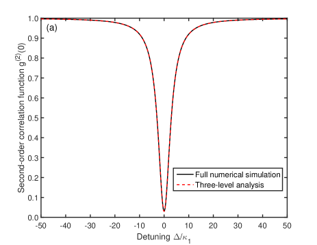
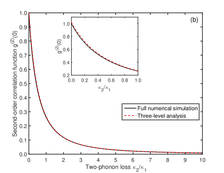
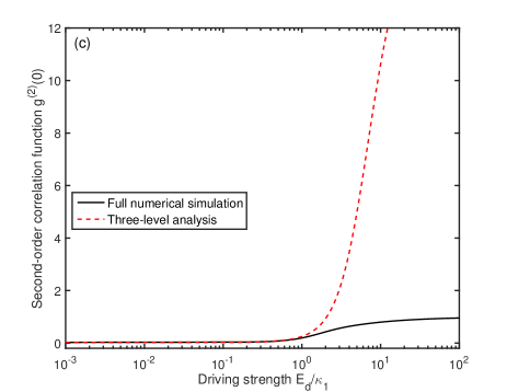
Figure 1: (a) Normalized zero-delay second-order correlation function $g^{(2)}(0)$ of the vdP oscillator plotted as a function of the dimensionless detuning $\Delta/\kappa_{1}$ for the two-phonon loss rate $\kappa_{2}/\kappa_{1}=5$ and the driving strength $E_{d}/\kappa_{1}=0.1$. (b) Dependence of zero-delay second-order correlation function $g^{(2)}(0)$ on the dimensionless two-phonon loss rate $\kappa_{2}/\kappa_{1}$, plotted for the zero detuning $\Delta/\kappa_{1}=0$ and the driving strength $E_{d}/\kappa_{1}=0.1$. The inset shows a zoom-in view of the $\kappa_{2}<\kappa_{1}$ region. (c) Dependence of zero-delay second-order correlation function $g^{(2)}(0)$ on the dimensionless driving strength $E_{d}/\kappa_{1}$ for changing logarithmically from $0.001$ to $100$, plotted for the zero detuning $\Delta/\kappa_{1}=0$ and the two-phonon loss rate $\kappa_{2}/\kappa_{1}=5$. In panels (a)-(c), the black solid lines denote full numerical simulations of a quantum master equation from Eq. (2), whereas the red dashed lines are analytical calculations of a three-oscillator-level model from Eq. (15).

Figure 1 shows the steady-state value of the normalized second-order correlation function at zero-time delay, $g^{(2)}(0)$, as a function of the detuning $\delta$ [panel (a)], the two-phonon loss $\kappa_{2}$ [panel (b)], and the driving strength $E_{d}$ [panel (c)], respectively. All plotted parameters are in units of the single-phonon loss $\kappa_{1}$ and thus are dimensionless. The black solid lines represent full numerical simulations from the quantum master equation (1), while the red dashed lines are analytical calculations predicted by Eq. (15) from the three-oscillator-level approximation. To be specific, it can be seen from Fig. 1(a) that the profile of the second-order correlation function $g^{(2)}(0)$ is symmetric with respect to the detuning $\Delta$. There is a marked antibunching dip at $\Delta=0$, corresponding to a minimum value of $g^{(2)}(0)\simeq 0.03$ in good agreement with Eq. (42). Increasing $|\Delta|$ leads to an increase in $g^{(2)}(0)$, degrading the degree of antibunching. For significantly large $|\Delta|$, $g^{(2)}(0)$ approaches a saturation value of unity, indicating coherent light emission. Numerical simulations matching analytical calculations show that the strong phonon antibunching can be achieved by utilizing the typical parameter values, e.g., $\kappa_{2}=5\kappa_{1}$ and $E_{d}=0.1\kappa_{1}$ given in Fig. 1(a), not specific values from any one experiment. In order to understand the physics behind this antibunching effect, intuitively, we look at the role of the $\kappa_{2}$ parameter, as will be discussed later.

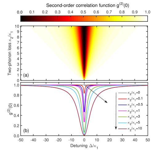
Figure 2: (a) 2D contour plot of normalized zero-delay second-order correlation function $g^{(2)}(0)$ versus the detuning $\Delta/\kappa_{1}$ and the two-phonon loss rate $\kappa_{2}/\kappa_{1}$ for the driving strength $E_{d}/\kappa_{1}=0.1$. (b) Cross section of (a) along the $\Delta$ axis, for seven fixed sets of the two-phonon loss rate $\kappa_{2}/\kappa_{1}=0$, $0.1$, $0.5$, $1$, $3$, $5$, and $10$.

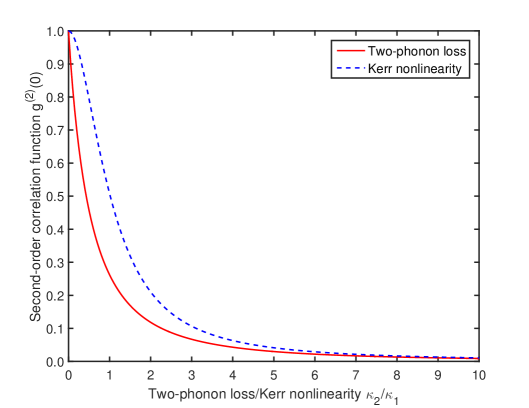
Figure 3: Comparison of the normalized second-order correlation function $g^{(2)}(0)$ obtained via the two-phonon loss in the vdP oscillator to that obtained via the Kerr nonlinearity in the resonator which only includes a single-phonon loss. Here the resulting effective Hamiltonian and the Lindblad master equation of the Kerr nonlinear resonator, respectively, are yielded by $\hat{H}_{KN}=\Delta\hat{a}^{{\dagger}}\hat{a}+\frac{1}{2}\kappa_{2}\hat{a}^{{\dagger}2}\hat{a}^{2}+iE_{d}(\hat{a}-\hat{a}^{{\dagger}})$ and $d\hat{\rho}/dt=-i[\hat{H}_{KN},\hat{\rho}]+\kappa_{1}D(\hat{a})\hat{\rho}$ in a rotating frame with respect to $\hat{H}_{0}=\omega_{d}\hat{a}^{{\dagger}}\hat{a}$. See main text about the vdP oscillator for more details. The other system parameters are set as $E_{d}/\kappa_{1}=0.1$ and $\Delta/\kappa_{1}=0$.

As illustrated in Fig. 1(b), when the two-phonon loss $\kappa_{2}$ is set to zero, $g^{(2)}(0)$ is equal to $1$, suggesting coherent light emitted from the vdP oscillator. Again, we can clearly see that $g^{(2)}(0)$ monotonically and rapidly decreases from $1$ as $\kappa_{2}$ increases, asymptotically approaching zero for large $\kappa_{2}$. For $\kappa_{2}\sim 0.4\kappa_{1}$, $g^{(2)}(0)$ can reach $0.5$. The value $g^{(2)}(0)<0.5$ is considered as an upper bound for single-phonon emission I-35b ; I-62 ; I-66 ; V-4 . As a consequence, the criterion for single-phonon emission can hold when $\kappa_{2}>0.4\kappa_{1}$. Such dissipative processes can be engineered in current experimental devices VI-1 ; VI-2 ; VI-15 , as will be illustrated in Sec. VI below. Note that, in Fig. 1(b), we keep the parameters $\Delta=0$ and $E_{d}=0.1\kappa_{1}$ fixed. In this scenario, the analytical $g^{(2)}(0)$ [black solid line in Fig. 1(b)] agrees very well with the numerically exact results [red dashed line in Fig. 1(b)]. Overall, the two-phonon loss dependence of phonon emission statistics shows that the degree of phonon antibunching can be kept high even for $\kappa_{2}<\kappa_{1}$.

In light of the above analyses from Figs. 1(a) and (b), we can conclude that the validity of such a three-oscillator-level approximation is not dependent on both the $\Delta$ and $\kappa_{2}$ parameters. What is the breakdown of this three-oscillator-level approximation? To help answer this question, in Fig. 1(c) we displays a typical case for varying the driving strength $E_{d}$ while keeping $\Delta=0$ and $\kappa_{2}=5\kappa_{1}$ fixed. Looking closer, we see that for small driving strengths in the range $E_{d}\leq\kappa_{1}$, this three-level analysis closely matches the result of the master equation simulation shown in Fig. 1(c). However, when the ratio $E_{d}/\kappa_{1}$ is larger than $1$, the three-level approximation completely fails to account for $g^{(2)}(0)$. With this fact, we notice from the black solid line of Fig. 1(c) that, as $E_{d}$ increases logarithmically from $0.001$ to $100$, $g^{(2)}(0)$ grows from a constant value close to zero, corresponding to single-phonon emission ($E_{d}\leq\kappa_{1}$), to an unity saturation value indicating coherent light emission ($E_{d}>80\kappa_{1}$). It is worth pointing out that strong antibunching [$g^{(2)}(0)\sim 0$] features a long plateau about $E_{d}$.

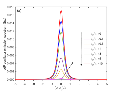
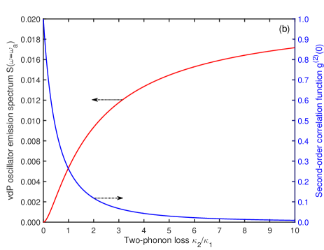
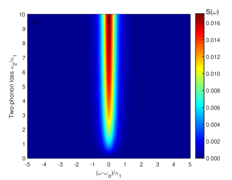
Figure 4: (a) Phonon emission spectrum $S(\omega)$ in arbitrary units, i.e., PSD as a function of the dimensionless frequency $(\omega-\omega_{d})/\kappa_{1}$ for a resonantly driven vdP oscillator in a frame rotating at the driving frequency $\omega_{d}$. The other system parameters are chosen as $E_{d}/\kappa_{1}=0.1$ and $\Delta/\kappa_{1}=0$, respectively. (b) Value of the spectrum $S(\omega=\omega_{a})$ at the vdP oscillator frequency $\omega_{a}$ as a function of the two-phonon loss rate $\kappa_{2}/\kappa_{1}$ on the left-hand axis. Zero-delay second-order correlation function $g^{(2)}(0)$ as a function of the two-phonon loss rate $\kappa_{2}/\kappa_{1}$ on the right-hand axis. The other system parameters are set as $E_{d}/\kappa_{1}=0.1$ and $\Delta/\kappa_{1}=0$. (c) 2D contour plot of vdP oscillator emission spectrum $S(\omega)$ (in arbitrary units) versus the frequency $(\omega-\omega_{d})/\kappa_{1}$ and the two-phonon loss rate $\kappa_{2}/\kappa_{1}$ for $E_{d}/\kappa_{1}=0.1$ and $\Delta/\kappa_{1}=0$.

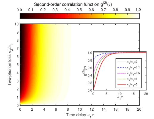
Figure 5: 2D contour plot of normalized second-order correlation function $g^{(2)}(\tau)$ with time delay $\tau$ as a function of the time delay $\kappa_{1}\tau$ and the two-phonon loss rate $\kappa_{2}/\kappa_{1}$ for the driving strength $E_{d}/\kappa_{1}=0.1$. The inset show the cross section of the main plot along the lateral axis, i.e., the time-delay dependence of the second-order correlation function $g^{(2)}(\tau)$, with the five different values of the two-phonon loss rate $\kappa_{2}/\kappa_{1}=0$, $0.1$, $0.5$, $1$, and $5$.

To gain further insight, Figure 2(a) displays the color-scale maps of the normalized second-order correlation function $g^{(2)}(0)$ as a function of both the detuning $\Delta$ and the two-phonon loss $\kappa_{2}$. Figure 2(b) shows the cuts through the horizontal $\Delta$-axis for seven different values of $\kappa_{2}$. It follows that the antibunching window width increases with increasing $\kappa_{2}$. Moreover, the degree of the antibunching is more pronounced as $\kappa_{2}$ is increased, whether the applied driving is set on resonance with the vdP oscillator or not. A natural question is, then, why the dissipation $\kappa_{2}$ plays an important role in generating phonon antibunching? As it is well known, the phonon dissipation offers a major source of decoherence V-5 ; V-6 ; V-7 ; V-10 , giving rise to the expectation that the dissipation should always weaken the antibunching. Physically, this is mainly because the two terms ($\frac{1}{2}\kappa_{2}a^{{\dagger}2}a^{{\dagger}2}\rho$ and $\frac{1}{2}\kappa_{2}\rho a^{{\dagger}2}a^{{\dagger}2}$) in the two-phonon dissipation expression of Eq. (1) act as the Kerr nonlinearity $\chi^{(3)}$ (see, for instance, Refs. V-8 ; V-9 ; VI-7 , and references therein). As an example, the dynamical evolution equations of the key field operator in the respective system are analogous; specifically, one is $\partial\hat{a}/\partial t=-i\Delta\hat{a}-\frac{1}{2}\kappa_{1}\hat{a}-\kappa_{2}\hat{a}^{{\dagger}}\hat{a}\hat{a}-E_{d}$ for the vdP oscillator, the other is $\partial\hat{a}/\partial t=-i\Delta\hat{a}-\frac{1}{2}\kappa_{1}\hat{a}-i\chi^{(3)}\hat{a}^{{\dagger}}\hat{a}\hat{a}-E_{d}$ for the Kerr nonlinear resonator. However, the present vdP oscillator for realizing the antibunching outperforms the Kerr nonlinear resonator when setting $\chi^{(3)}=\kappa_{2}$ and the other common parameters are the same as in Fig. 1(a), as verified from Fig. 3. A striking feature of the results of Fig. 3 is the fact that, for an identical $\kappa_{2}$, the degree of the phonon antibunching for the vdP oscillator is much smaller than that for the Kerr nonlinear resonator. Thus, the antibunching phenomenon is more pronounced relative to the Kerr nonlinear resonator.

In the following, we elaborate on the amount of phonon emission through the vdP oscillator corresponding to the driving used in Figs. 1(a) and (b), as we collect the fluorescence primarily from the oscillator. These would be of interest in designing a practical experiment, as it would be of consequence to the number of counts that are obtained in the correlation measurement. To this end, the fluorescence phonon emission spectrum of the vdP oscillator is yielded by the power spectral density (PSD), which is defined as the Fourier transform of the first-order correlation function of the vdP oscillator field, namely, $S(\omega)=\int_{-\infty}^{\infty}\langle\hat{a}^{{\dagger}}(\tau)\hat{a}(0)\rangle e^{-i(\omega-\omega_{d})\tau}d\tau$ V-5 ; V-6 ; V-7 , where the angular brackets represent the average in the steady state of Eq. (2) and the calculation is performed in the frame rotating with the driving frequency $\omega_{d}$. The PSD of the vdP mode can be directly monitored in experiments.

In Fig. 4(a), we display the calculated phonon emission spectra $S(\omega)$ as a function of the frequency $\omega$ for seven different values of the two-phonon loss $\kappa_{2}$. As can be seen, the phonon emission spectra possess a symmetrical single-peak structure, which is of typical Lorentzian shape reminiscent of a weakly driven two-level system V-5 . The peak values are located at $\omega=\omega_{d}$, indicating synchronization to the external driving. Here it is worth pointing out that, without the nonlinear two-phonon loss and only with the linear single-phonon loss corresponding to the case of $\kappa_{2}/\kappa_{1}=0$ in Fig. 4(a), the spectral line is flat and the phonon emission output is almost equal to zero. This is due to the fact that the applied driving field is considerably weak, $E_{d}=0.1\kappa_{1}$ in this linear oscillator system. When $E_{d}$ is comparable to $\kappa_{1}$, the phonon emission output, with a Lorentzian shape and a linewidth given by $\kappa_{1}$, can occur (not shown). With increasing $\kappa_{2}$, the amount of phonon emission is enhanced distinctly owing to the presence and raise of the nonlinearity. Correspondingly, the spectral width of the emission is increased. For gradually increasing $\kappa_{2}$ from a zero value, the steady-state occupations of all Fock states (including $|1\rangle$) decrease since there is an additional relaxation channel opened, as is also confirmed by Eqs. (25) and (26) or Eqs. (40) and (41). Therefore, with increasing the $\kappa_{2}/\kappa_{1}$ ratio we can expect an increasing spectral width and emission amplitude.

In Fig. 4(b), we plot the amount of phonon emission $S(\omega=\omega_{a})$ on the vdP oscillator resonance with the driving (i.e., $\Delta=0$) as a function of $\kappa_{2}$ (left scale). $S(\omega=\omega_{a})$ rises up quickly with $\kappa_{2}$. For the sake of direct comparison with the above emission amount, again we show the second-order correlation function $g^{(2)}(0)$ in Fig. 4(b) (right scale). It is evident from these plots that the changes of $S(\omega=\omega_{a})$ are opposite to $g^{(2)}(0)$; strong phonon antibunching is accompanied by the high amount of phonon emission, which is beneficial to the $g^{(2)}(0)$ measurement in practical experiments. For the sake of clarity, we depict contour plot of $S(\omega)$ as a function of $\omega$ and $\kappa_{2}$ in Fig. 4(c), the cuts of which through the horizontal axis correspond to Fig. 4(a). In a word, the stronger the antibunching is, the higher the collected fluorescence (the power spectral density) is, as expected.

For all the discussions above, so far we only consider the zero-time-delay second-order correlation function $g^{(2)}(0)$. Now we focus on $g^{(2)}(\tau)$ with time delay $\tau$. Figure 5 depicts the behavior of $g^{(2)}(\tau)$ as a function of both the time delay $\tau$ and the two-phonon loss $\kappa_{2}$ in a 2D contour plot. The inset in the main plot intuitively displays $g^{(2)}(\tau)$ versus $\tau$ for various values of $\kappa_{2}$ shown in the legend. Note that, the delayed $g^{(2)}(\tau)$ is only computed for $\tau\geq 0$, because it is formally symmetric about $\tau=0$, i.e., $g^{(2)}(-\tau)=g^{(2)}(\tau)$ as mentioned before. We see from these figures that $g^{(2)}(\tau)$ monotonically increases from a value smaller than $1$ (indicating antibunched phonon emission) to $1$ (indicating coherent phonon emission) with $\tau$ for a given nonzero value of $\kappa_{2}$. In particular, for $\kappa_{2}=0$, $g^{(2)}(\tau)$ is identically equal to $1$. For a sufficient $\tau$, $g^{(2)}(\tau)$ reaches the value of $1$. Most obviously, a minimum value of $g^{(2)}(\tau)$ is obtained at $\tau=0$. The minimum value of $g^{(2)}(\tau)$ diminishes with increasing $\kappa_{2}$. Also, $g^{(2)}(\tau)$ persists at some value below unity over a long time, on the order of $1/\kappa_{1}$. From another point of view, it is found from Fig. 5 that the relationship $g^{(2)}(\tau)>g^{(2)}(0)$ is always satisfied for $\kappa_{2}\neq 0$, which violates the Cauchy-Schwarz inequality $g^{(2)}(\tau)\leq g^{(2)}(0)$ related to classical light and thus shows the phenomenon of phonon antibunching or sub-Poissonian statistics related to nonclassical light V-5 ; V-6 ; V-7 ; V-10 .

VI Feasibility of experimentally implementing a quantum vdP oscillator

Regarding the experimental feasibility of our scheme, we note that two typical setups, (i) an ion trap VI-1 ; VI-2 ; VI-3 ; VI-4 ; VI-5 ; VI-6 ; VI-7 and (ii) an optomechanical membrane VI-8 ; VI-9 ; VI-10 , have demonstrated the possibility of implementing a vdP oscillator. First, for the ion trap setup proposed originally in Refs. VI-1 ; VI-2 , the oscillator mode $\hat{a}$ in Eq. (1) stands for a linearly damped motional degree of freedom of the trapped ion. Correspondingly, the linear one-phonon damping can occur when the standard laser cooling techniques are utilized VI-8 . One can engineer the nonlinear damping via applying sideband transitions to remove energy quanta, for example, the two-phonon loss can be carried out by laser exciting a harmonically trapped ion to its red motional sideband by removing two phonons at a time VI-1 ; VI-2 . In this scenario, the one- and two-phonon loss rates are both of the order of kHz, with $\kappa_{2}\geq\kappa_{1}$ VI-1 ; VI-2 ; VI-3 ; VI-6 ; VI-7 . As also shown in Refs. VI-1 ; VI-7 , it is possible to resolve sidebands and suppress off-resonant excitations for several tens of low-energy modes.

Second, for the optomechanical “membrane-in-the-middle” system VI-9 ; VI-10 ; VI-11 or the mechanical self-oscillation in cavity optomechanical system VI-12 ; VI-13 ; VI-14 , one can take into account a moderate quality factor membrane with the linear mechanical damping. The nonlinear two-phonon damping can be implemented by exploiting a laser red-detuned with two mechanical frequencies relative to the two-phonon sideband. One can apply an electric field gradient created near the membrane to create the driving force.

As a side note, the present phonon mode can be extended to a stationary photonic mode in an optical system, such as a microwave resonator or an optical cavity. Strong two-photon loss can also be realized successfully through the Josephson junction in superconducting circuit with high tunability VI-15 or through using an on-chip toroidal microcavity immersed in rubidium vapor I-74 .

Finally, one can use the objective to collect the phonon or photon emission from the oscillator mode $\hat{a}$. Then it is sent to a Hanbury-Brown–Twiss (HBT) configuration, consisting of a $50:50$ beam splitter and a pair of single-phonon or single-photon counting detectors. The normalized second-order correlation function of interest, characterizing the quantum statistics of particle sources, can be measured by this HBT setup (see, for instance, Refs. V-5 ; V-6 ; V-7 , and references therein). Thus, we expect that an experimental implementation of our scheme is feasible in the present state of the art.

VII Conclusions

In summary, we have introduced an alternative route towards highly nonclassical phonon emission statistics in a driven quantum vdP oscillator subject to both the linear one-phonon and nonlinear two-phonon damping by evaluating the second-order correlation function $g^{(2)}$ numerically and analytically. With experimentally achievable parameters, strong antibunching in the emitted phonon statistics is revealed by the full numerical simulations using a quantum master equation, which is in good agreement with analytical calculations utilizing a three–vdP-oscillator–level model by assuming that only the three lowest Fock states of the vdP oscillator have non-negligible occupations under weak driving. It is shown that the degree of phonon antibunching is limited by the rate of the two-phonon loss in this vdP oscillator, and the antibunching is enhanced considerably with growing the two-phonon loss. So, the two-phonon loss is very important for the realization of a good single-phonon device. The degree of phonon antibunching can be kept high even when $\kappa_{2}<\kappa_{1}$. Suitable conditions for strong phonon antibunching generation and single-phonon emission are identified in the parameter regimes. On the other hand, we also numerically calculate the fluorescence phonon emission spectra $S(\omega)$, given by the power spectral density of the driven vdP oscillator. We further find that high phonon emission amplitudes, simultaneously accompanied by strong phonon antibunching, can be obtained, which are beneficial to the HBT measurement of the emitted phonons in practical experiments. Lastly, following the original proposals in Refs. VI-1 ; VI-2 , we illustrate specific implementations applying a harmonically trapped ion and an optomechanical membrane in the middle. Our model’s description of the interplay between one-phonon and two-phonon losses and their effects is not limited to phononic systems and should be generally applicable to photonic systems. This vdP architecture provides a feasible way of realizing efficient single-phonon or single-photon sources for quantum information processing tasks.

Data Availability

The data that support the findings of this study are available from the corresponding author upon reasonable request.

References

- (1) A. Imamoglu, H. Schmidt, G. Woods, and M. Deutsch, Strongly Interacting Photons in a Nonlinear Cavity, Phys. Rev. Lett. 79, 1467–1470 (1997).
- (2) K. M. Birnbaum, A. Boca, R. Miller, A. D. Boozer, T. E. Northup, and H. J. Kimble, Photon blockade in an optical cavity with one trapped atom, Nature (London) 436, 87–90 (2005).
- (3) K. Hennessy, A. Badolato, M. Winger, D. Gerace, M. Atatüre, S. Gulde, S. Fält, E. L. Hu, and A. Imamoglu, Quantum nature of a strongly coupled single quantum dot-cavity system, Nature (London) 445, 896–899 (2007).
- (4) A. Faraon, I. Fushman, D. Englund, N. Stoltz, P. Petroff, and J. Vučković, Coherent generation of non-classical light on a chip via photon-induced tunnelling and blockade, Nat. Phys. 4, 859–863 (2008).
- (5) A. Reinhard, T. Volz, M. Winger, A. Badolato, K. J. Hennessy, E. L. Hu, and A. Imamoǧlu, Strongly correlated photons on a chip, Nat. Photon. 6, 93–96 (2012).
- (6) K. Müller, A. Rundquist, K. A. Fischer, T. Sarmiento, K. G. Lagoudakis, Y. A. Kelaita, C. S. Muñoz, E. del Valle, F. P. Laussy, and J. Vučković, Coherent Generation of Nonclassical Light on Chip via Detuned Photon Blockade, Phys. Rev. Lett. 114, 233601 (2015).
- (7) C. Hamsen, K. N. Tolazzi, T. Wilk, and G. Rempe, Two-Photon Blockade in an Atom-Driven Cavity QED System, Phys. Rev. Lett. 118, 133604 (2017).
- (8) M. Radulaski, K. A. Fischer, and J. Vučković, Nonclassical Light Generation From III-V and Group-IV Solid-State Cavity Quantum Systems, in Advances in Atomic, Molecular, and Optical Physics (Academic Press, New York, 2017), Vol. 66, pp. 111–179.
- (9) T. C. H. Liew and V. Savona, Single photons from coupled quantum modes, Phys. Rev. Lett. 104, 183601 (2010).
- (10) M. Bamba, A. Imamoǧlu, I. Carusotto, and C. Ciuti, Origin of strong photon antibunching in weakly nonlinear photonic molecules, Phys. Rev. A 83, 021802(R) (2011).
- (11) For recent reviews, see E. Zubizarreta Casalengua, J. C. López Carreño, F. P. Laussy, and E. del Valle, Conventional and Unconventional Photon Statistics, Laser Photonics Rev. 14, 1900279 (2020).
- (12) For recent reviews, see R. Trivedi, K. A. Fischer, J. Vučković, and K. Müller, Generation of Non-Classical Light Using Semiconductor Quantum Dots, Adv. Quantum Technol. 3, 1900007 (2020).
- (13) H. Jing, S. K. Özdemir, X.-Y Lü, J. Zhang, L. Yang, and F. Nori, -Symmetric Phonon Laser, Phys. Rev. Lett. 113, 053604 (2014).
- (14) M. R. Hush, W. Li, S. Genway, I. Lesanovsky, and A. D. Armour, Phys. Rev. A 91, 061401(R) (2015).
- (15) T.-S. Yin, Q. Bin, G.-L. Zhu, G.-R. Jin, and A. Chen, Phys. Rev. A 100, 063840 (2019).
- (16) H. Xie, C.-G. Liao, X. Shang, Z.-H. Chen, and X.-M. Lin, Phys. Rev. A 98, 023819 (2018).
- (17) Y. X. Liu, A. Miranowicz, Y. B. Gao, J. Bajer, C. P. Sun, and F. Nori, Qubit-induced phonon blockade as a signature of quantum behavior in nanomechanical resonators, Phys. Rev. A 82, 032101 (2010).
- (18) T. Ramos, V. Sudhir, K. Stannigel, P. Zoller, and T. J. Kippenberg, Nonlinear Quantum Optomechanics via Individual Intrinsic Two-Level Defects, Phys. Rev. Lett. 110, 193602 (2013).
- (19) X. Wang, A. Miranowicz, H. R. Li, and F. Nori, Method for observing robust and tunable phonon blockade in a nanomechanical resonator coupled to a charge qubit, Phys. Rev. A 93, 063861 (2016).
- (20) X.-W. Xu, A.-X. Chen, and Y.-x. Liu, Phonon blockade in a nanomechanical resonator resonantly coupled to a qubit, Phys. Rev. A 94, 063853 (2016).
- (21) H. Seok and E. M. Wright, Antibunching in an optomechanical oscillator, Phys. Rev. A 95, 053844 (2017).
- (22) N. Lörch and K. Hammerer, Sub-Poissonian phonon lasing in three-mode optomechanics, Phys. Rev. A 91, 061803(R) (2015).
- (23) L.-L. Zheng, T.-S. Yin, Q. Bin, X.-Y. Lü, and Y. Wu, Single-photon-induced phonon blockade in a hybrid spin-optomechanical system, Phys. Rev. A 99, 013804 (2019).
- (24) B. van der Pol, LXXXVIII. On “relaxation-oscillations,” Philos. Mag. 2, 978–992 (1926).
- (25) T. E. Lee and H. R. Sadeghpour, Quantum Synchronization of Quantum van der Pol Oscillators with Trapped Ions, Phys. Rev. Lett. 111, 234101 (2013).
- (26) S. Walter, A. Nunnenkamp, and C. Bruder, Quantum Synchronization of a Driven Self-Sustained Oscillator, Phys. Rev. Lett. 112, 094102 (2014).
- (27) N. Lörch, E. Amitai, A. Nunnenkamp, and C. Bruder, Genuine Quantum Signatures in Synchronization of Anharmonic Self-Oscillators, Phys. Rev. Lett. 117, 073601 (2016).
- (28) C. Navarrete-Benlloch, T. Weiss, S. Walter, and G. J. de Valcárcel, General Linearized Theory of Quantum Fluctuations around Arbitrary Limit Cycles, Phys. Rev. Lett. 119, 133601 (2017).
- (29) T. Weiss, S. Walter, and F. Marquardt, Quantum-coherent phase oscillations in synchronization, Phys. Rev. A 95, 041802(R) (2017).
- (30) S. Sonar, M. Hajdušek, M. Mukherjee, R. Fazio, V. Vedral, S. Vinjanampathy, and L.-C. Kwek, Squeezing Enhances Quantum Synchronization, Phys. Rev. Lett. 120, 163601 (2018).
- (31) S. Dutta and N. R. Cooper, Critical Response of a Quantum van der Pol Oscillator, Phys. Rev. Lett. 123, 250401 (2019).
- (32) T. Weiß, Nonlinear dynamics in quantum synchronization and topological transport, Dissertation, 2017. https://opus4.kobv.de/opus4-fau/files/8704/TalithaWeissDissertation.pdf
- (33) E. Amitai, Phase and amplitude dynamics of quantum self-oscillators, Dissertation, 2018. https://edoc.unibas.ch/64965/1/Dissertation
- (34) T. E. Lee, C.-K. Chan, and S. Wang, Entanglement tongue and quantum synchronization of disordered oscillators, Phys. Rev. E 89, 022913 (2014).
- (35) S. Walter, A. Nunnenkamp, and C. Bruder, Quantum synchronization of two Van der Pol oscillators, Ann. Phys. (Berlin) 527, 131–138 (2015).
- (36) M. R. Jessop, W. Li, and A. D. Armour, Phase synchronization in coupled bistable oscillators, arXiv:1906.07603v2 [quant-ph].
- (37) E. Amitai, M. Koppenhöfer, N. Lörch, and C. Bruder, Quantum effects in amplitude death of coupled anharmonic self-oscillators, Phys. Rev. E 97, 052203 (2018).
- (38) J. I. Cirac, R. Blatt, P. Zoller, and W. D. Phillips, Laser cooling of trapped ions in a standing wave, Phys. Rev. A 46, 2668–2681 (1992).
- (39) A. Jayich, J. Sankey, B. Zwickl, C. Yang, J. Thompson, S. Girvin, A. Clerk, F. Marquardt, and J. Harris, Dispersive optomechanics: a membrane inside a cavity, New J. Phys. 10, 095008 (2008).
- (40) J. D. Thompson, B. M. Zwickl, A. M. Jayich, F. Marquardt, S. M. Girvin, and J. G. E. Harris, Strong dispersive coupling of a high-finesse cavity to a micromechanical membrane, Nature (London) 452, 72–75 (2008).
- (41) N. Bartolo, F. Minganti, W. Casteels, and C. Ciuti, Exact steady state of a Kerr resonator with one- and two-photon driving and dissipation: Controllable Wigner-function multimodality and dissipative phase transitions, Phys. Rev. A 94, 033841 (2016).
- (42) N. Bartolo, F. Minganti, J. Lolli, and C. Ciuti, Homodyne versus photon-counting quantum trajectories for dissipative Kerr resonators with two-photon driving, Eur. Phys. J. Spec. Top. 226, 2705–2713 (2017).
- (43) F. Minganti, N. Bartolo, J. Lolli, W. Casteels, and C. Ciuti, Exact results for Schrödinger cats in driven-dissipative systems and their feedback control, Sci. Rep. 6, 26987 (2016).
- (44) M. O. Scully and M. S. Zubairy, Quantum Optics (Cambridge University Press, Cambridge, 1997).
- (45) C. Gardiner and P. Zoller, Quantum Noise: A Handbook of Markovian and Non-Markovian Quantum Stochastic Methods with Applications to Quantum Optics (Springer, Berlin, 2004).
- (46) G. S. Agarwal, Quantum Optics (Cambridge University Press, Cambridge, 2013).
- (47) H.-P. Breuer and F. Petruccione, The Theory of Open Quantum Systems (Oxford University Press, Oxford, 2002).
- (48) M. Arcari, I. Söllner, A. Javadi, S. Lindskov Hansen, S. Mahmoodian, J. Liu, H. Thyrrestrup, E. H. Lee, J. D. Song, S. Stobbe, and P. Lodahl, Near-Unity Coupling Efficiency of a Quantum Emitter to a Photonic Crystal Waveguide, Phys. Rev. Lett. 113, 093603 (2014).
- (49) H. Flayac and V. Savona, Unconventional Photon Blockade, Phys. Rev. A 96, 053810 (2017).
- (50) H. Flayac and V. Savona, Single photons from dissipation in coupled cavities, Phys. Rev. A 94, 013815 (2016).
- (51) J. Gallego, W. Alt, T. Macha, M. Martinez-Dorantes, D. Pandey, and D. Meschede, Strong Purcell Effect on a Neutral Atom Trapped in an Open Fiber Cavity, Phys. Rev. Lett. 121, 173603 (2018).
- (52) Z. Leghtas, S. Touzard, I. M. Pop, A. Kou, B. Vlastakis, A. Petrenko, K. M. Sliwa, A. Narla, S. Shankar, M. J. Hatridge, M. Reagor, L. Frunzio, R. J. Schoelkopf, M. Mirrahimi, and M. H. Devoret, Confining the state of light to a quantum manifold by engineered two-photon loss, Science 347, 853–857 (2015).
- (53) A. Nunnenkamp, K. Børkje, J. G. E. Harris, and S. M. Girvin, Cooling and squeezing via quadratic optomechanical coupling, Phys. Rev. A 82, 021806(R) (2010).
- (54) F. Marquardt, J. G. E. Harris, and S. M. Girvin, Dynamical multistability induced by radiation pressure in high-finesse micromechanical optical cavities, Phys. Rev. Lett. 96, 103901 (2006).
- (55) T. J. Kippenberg, H. Rokhsari, T. Carmon, A. Scherer, and K. J. Vahala, Analysis of radiation-pressure induced mechanical oscillation of an optical microcavity, Phys. Rev. Lett. 95, 033901 (2005).
- (56) C. Metzger, M. Ludwig, C. Neuenhahn, A. Ortlieb, I. Favero, K. Karrai, and F. Marquardt, Self-induced oscillations in an optomechanical system driven by bolometric backaction, Phys. Rev. Lett. 101, 133903 (2008).
- (57) Y.-P. Huang and P. Kumar, Antibunched Emission of Photon Pairs via Quantum Zeno Blockade, Phys. Rev. Lett. 108, 030502 (2012).