Tidal effects in Schwarzschild black hole in holographic massive gravity

Abstract

We investigate tidal effects produced in the spacetime of Schwarzschild black hole in holographic massive gravity, which has two additional mass parameters due to massive gravitons. As a result, we have obtained that massive gravitons affect the angular component of the tidal force, while the radial component has the same form with the one in massless gravity. On the other hand, by solving the geodesic deviation equations, we have found that radial components of two nearby geodesics keep tightening while falling into the black hole and after passing the event horizons get abruptly infinitely stretched due to massive gravitons. However, angular components of two nearby geodesics get stretched firstly, reach a peak and then get compressed while falling into the black hole. Moreover, we have also shown that the angular components are more easily deformed near the departure position as the mass of a black hole is smaller for a fixed graviton mass.

I introduction

Einstein’s theory of general relativity (GR) has been tested successfully to date as the description of the force of gravity. Despite all the successes of GR, some puzzles not only on cosmological scales but also on quantum scales have pushed forward to search for alternatives. Various modifications are obtained by adding extra scalar, vector, or tensor fields to their gravitational sector, and additional scalar curvature invariants to the action of GR Clifton:2011jh .

In particular, introducing extra tensor fields as a background can make Einstein’s massless spin-2 graviton to be massive Hinterbichler:2011tt ; deRham:2014zqa . For example, a massive spin-2 theory can be considered as a theory with a dynamical fluctuation on a nondynamical background. Taking the background tensor to be the Minkowskian one, one can have a massive graviton by adding the Pauli-Fierz mass term to the GR action, resulting in the Pauli-Fierz action Fierz:1939ix . However, it was later known that the massive gravity suffered from the Boulware-Deser ghost problem Boulware:1973my and the van Dam, Veltman and Zakharov (vDVZ) discontinuity vanDam:1970vg ; Zakharov:1970cc in the massless graviton limit.

A decade ago, de Rham, Gabadadze and Trolley (dRGT) deRham:2010ik ; deRham:2010kj obtained a ghost free massive gravity, which has nonlinearly interacting mass terms constructed from the metric coupled with a symmetric background tensor, called the reference metric. In the dRGT massive gravity, the nondynamical background tensor is also set to be the Minkowskian one. In order to preserve diffeomorphism invariance, Hassan et al. Hassan:2011hr ; Hassan:2011tf developed the ghost free massive gravity with a general reference metric. On the other hand, Vegh Vegh:2013sk introduced a nonlinear massive gravity with a special singular reference metric as a background tensor, which is used to study momentum dissipation for describing the electric and heat conductivity for normal conductors. The nondynamical background tensor is chosen to keep the diffeomorphism symmetry for coordinates ($t,r$) intact, but breaks it in angular directions. Due to a broken momentum conservation, graviton acquires the mass that leads to momentum dissipation in the dual holographic theory. Thus, massive gravity theories with broken diffeomorphism invariance in the bulk provide a holographic model for theories with broken spatial translational symmetry at the boundary Davison:2013jba ; Blake:2013bqa ; Blake:2013owa . Since then, this has been extensively exploited to investigate many black hole models Cai:2014znn ; Adams:2014vza ; Hendi:2015pda ; Hu:2016hpm ; Zou:2016sab ; Hendi:2017fxp ; Tannukij:2017jtn ; Hendi:2017bys ; Hendi:2018xuy ; Chabab:2019mlu ; Hong:2018spz ; Hong:2019zsi as well as holographic condensed matter physics Andrade:2013gsa ; Amoretti:2014zha ; Baggioli:2014roa ; Zhou:2015dha ; Hartnoll:2016apf ; Alberte:2017oqx ; Ammon:2019wci . In addition, it was also studied what effects of the holographic massive gravity were on the structure of physical neutron stars Hendi:2017ibm .

On the other hand, it is well-known that a body in free fall toward the center of another body gets stretched in the radial direction and compressed in the angular one. The stretching and compression arise from a tidal effect of gravity, which is given by a difference in the strength of gravity between two points MTW:1973 ; DInverno:1992 ; Carroll:2004 ; Hobson:2006 . Tidal phenomena are common in the universe from our solar system to stars in binary systems, to galaxies, to cluster of galaxies, and even to gravitational waves Goswami:2019fyk . In particular, Wheeler Wheeler:1971 proposed that a star in the ergosphere of the Kerr black hole can be broken up due to tidal interaction and emit subsequently a jet composed of the debris as a mechanism for the jets production. Since then, the investigation of tidal effects in astrophysical context has been devoted to tidal disruption of stars deeply plunging into black holes Hills:1975 ; Carter:1982 ; Rees:1988 ; komossa:2015 ; Auchettl:2017 ; Rossi:2020rvv . Many other studies in theoretical context have also been preformed for the extensive description of tidal effects in various black holes Mahajan:1981 ; AbdelMegied:2004ni ; Crispino:2016pnv ; Gad2010 ; Shahzad:2017vwi ; Chan:1995fc ; Nandi:2000gt ; Cardoso:2012zn ; Harko:2012ve ; Uniyal:2014oaa ; Sharif:2018a ; Sharif:2018gzj ; Junior:2020yxg ; Junior:2020par . Very recently, making use of a tidal acceleration of the separation between two arms of gravitational wave detectors such as LIGO Abbott:2016blz ; Abbott:2017vtc , the authors have proposed a new method of a direct measurement of gravitons Parikh:2020nrd ; Parikh:2020kfh ; Parikh:2020fhy .

However, studies on tidal effects in astrophysical context so far have been mainly devoted to either the nonrotating Schwarzschild or the rotating Kerr black holes in massless gravity. Moreover, in theoretical context, even though tidal effects have also been studied in various black holes, there are few works on possible deformation of geodesic deviation vectors when the metric is changed according to massive graviton.

Motivated by this, we will study tidal effects in the Schwarzschild black hole in Vegh’s holographically massive gravity, which has two additional mass parameters due to massive gravitons, comparing them with the Schwarzschild black hole in massless gravity. In Sec. II and III, we investigate features of the geodesic equations and tidal forces for the Schwarzschild black hole in holographic massive gravity. In Sec. IV, we find solutions of the geodesic deviation equations for radially falling bodies toward the Schwarzschild black hole in holographic massive gravity and analyze the results having massive gravitons comparing with the ones in massless gravity. Conclusions are drawn in Sec. V.

II Geodesics in Schwarzschild black hole in holographic massive gravity

In this section, we will newly study the geodesic equations of Schwarzschild black hole in holographic massive gravity, which is described by the action

$$S=\frac{1}{16\pi G}\int d^{4}x\sqrt{-g}\left[{\cal R}+{\tilde{m}}^{2}\sum_{i=1}^{4}a_{i}{\cal U}_{i}(g_{\mu\nu},f_{\mu\nu})\right],$$ (2.1)

where ${\cal R}$ is the scalar curvature, $\tilde{m}$ is the graviton mass, $a_{i}$ are constants and ${\cal U}_{i}$ are symmetric polynomials of the eigenvalue of the matrix ${\cal K}^{\mu}_{\nu}\equiv\sqrt{g^{\mu\alpha}f_{\alpha\nu}}$ given by

$${\cal U}_{1} = [{\cal K}],~{}~{}~{}{\cal U}_{2}=[{\cal K}]^{2}-[{\cal K}^{2}],~{}~{}~{}{\cal U}_{3}=[{\cal K}]^{3}-3[{\cal K}][{\cal K}^{2}]+2[{\cal K}^{3}]$$

$${\cal U}_{4} = [{\cal K}]^{4}-6[{\cal K}^{2}][{\cal K}]^{2}+8[{\cal K}^{3}][{\cal K}]+3[{\cal K}^{2}]^{2}-6[{\cal K}^{4}].$$ (2.2)

The square root in ${\cal K}$ means $(\sqrt{A})^{\mu}_{\alpha}(\sqrt{A})^{\alpha}_{\nu}=A^{\mu}_{\nu}$ and $[{\cal K}]$ denotes the trace ${\cal K}^{\mu}_{\mu}$. Finally, $f_{\mu\nu}$, called the reference metric, is a non-dynamical, fixed symmetric tensor introduced to construct nontrivial interaction terms in holographic massive gravity. Then, with a gauge-fixed ansatz for the reference metric as

$$f_{\mu\nu}={\rm diag}(0,0,a^{2}_{0},a^{2}_{0}\sin^{2}\theta),$$ (2.3)

where $a_{0}$ is a positive constant Vegh:2013sk ; Blake:2013bqa ; Amoretti:2014zha ; Zhou:2015dha ; Cai:2014znn ; Adams:2014vza ; Hong:2018spz ; Hong:2019zsi , one can find the spherically symmetric black hole solution as

$$ds^{2}=g_{\mu\nu}dx^{\mu}dx^{\nu}=-f(r)dt^{2}+f^{-1}(r)dr^{2}+r^{2}(d\theta^{2}+\sin^{2}\theta d\phi^{2})$$ (2.4)

with

$$f(r)=1-\frac{2m}{r}+2Rr+{\cal C}.$$ (2.5)

Here, we have newly defined $R=a_{0}a_{1}\tilde{m}^{2}/4$ and ${\cal C}=a^{2}_{0}a_{2}\tilde{m}^{2}$ without loss of generality.

In order to see the difference between the Schwarzschild black holes in holographic massive gravity and in massless one, we have drawn the mass parameter dependent Hawking temperature in Fig. 1

$$T_{H}=\frac{1+{\cal C}}{4\pi r_{H}}+\frac{R}{\pi},$$ (2.6)

which shows the role of two additional mass terms $R$ and ${\cal C}$ clearly. As seen from Fig. 1, the Hawking temperature in the holographic massive gravity differently behaves according to the values of ${\cal C}$ and $R$. Note that first $R$ gives a constant contribution to the Hawking temperature. The Hawking temperature is mostly proportional to $1/r_{H}$. When ${\cal C}>-1$, it decreases as $r_{H}$ increases. When ${\cal C}=-1$, it is just a constant given by $R$. However, when ${\cal C}<-1$, it is negatively proportional to $1/r_{H}$. Note that the Hawking temperature is flipped by the sign of $\cal C$. In this paper, we assume that the mass parameters are positive without loss of generality.

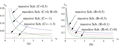
Figure 1: Hawking temperature for the Schwarzschild black hole in holographic massive gravity: (a) varying $\cal C$ with $R=0.1$ and (b) varying $R$ with $C=0.3$, comparing with ones in massless gravity.

Now, the geodesic equations of

$$\frac{d^{2}x^{\mu}}{d\tau^{2}}+\Gamma^{\mu}_{\nu\rho}\frac{dx^{\nu}}{d\tau}\frac{dx^{\rho}}{d\tau}=0$$ (2.7)

can be obtained from the metric where $x^{\mu}=(t,r,\theta,\phi)$. Here, the independent non-vanishing components of the Christoffel symbols are

$$\Gamma^{0}_{01} = -\Gamma^{1}_{11}=\frac{f^{\prime}(r)}{2f(r)},~{}~{}~{}\Gamma^{1}_{00}=\frac{1}{2}f^{\prime}(r)f(r),~{}~{}~{}~{}~{}\Gamma^{1}_{22}=-rf(r),~{}~{}~{}\Gamma^{1}_{33}=-rf(r)\sin^{2}\theta,$$

$$\Gamma^{2}_{12} = \Gamma^{3}_{13}=\frac{1}{r},~{}~{}~{}~{}~{}~{}~{}~{}~{}~{}~{}\Gamma^{2}_{33}=-\sin\theta\cos\theta,~{}~{}~{}~{}\Gamma^{3}_{23}=\cot\theta.$$ (2.8)

From these equations, one can explicitly obtain the geodesic equations as

$$\frac{dv^{0}}{d\tau}+\frac{2(m+Rr^{2})}{r^{2}-2mr+2Rr^{3}+{\cal C}r^{2}}v^{0}v^{1}=0,$$ (2.9)

$$\frac{dv^{1}}{d\tau}+\frac{(m+Rr^{2})}{r^{4}}(r^{2}-2mr+2Rr^{3}+{\cal C}r^{2})(v^{0})^{2}-\frac{m+Rr^{2}}{r^{2}-2mr+2Rr^{3}+{\cal C}r^{2}}(v^{1})^{2}$$

$$-\frac{r^{2}-2mr+2Rr^{3}+{\cal C}r^{2}}{r}[(v^{2})^{2}+\sin^{2}\theta(v^{3})^{2}]=0,$$ (2.10)

$$\frac{dv^{2}}{d\tau}+\frac{2}{r}v^{1}v^{2}-\sin\theta\cos\theta(v^{3})^{2}=0,$$ (2.11)

$$\frac{dv^{3}}{d\tau}+\frac{2}{r}v^{1}v^{3}+\cot\theta v^{2}v^{3}=0$$ (2.12)

in terms of the four velocity vector $v^{\mu}=dx^{\mu}/d\tau$. Without loss of generality, one can consider the geodesics on the equatorial plane $\theta=\pi/2$ for all $\tau$. Then, one has $v^{2}=\dot{\theta}=0$ and the geodesic equations are finally reduced to

$$\frac{dv^{0}}{d\tau}+\frac{2(m+Rr^{2})}{r^{2}-2mr+2Rr^{3}+{\cal C}r^{2}}v^{0}v^{1}=0,$$ (2.13)

$$\frac{dv^{1}}{d\tau}+\frac{(m+Rr^{2})}{r^{4}}(r^{2}-2mr+2Rr^{3}+{\cal C}r^{2})(v^{0})^{2}-\frac{m+Rr^{2}}{r^{2}-2mr+2Rr^{3}+{\cal C}r^{2}}(v^{1})^{2}$$

$$-\frac{r^{2}-2mr+2Rr^{3}+{\cal C}r^{2}}{r}(v^{3})^{2}=0,$$ (2.14)

$$\frac{dv^{3}}{d\tau}+\frac{2}{r}v^{1}v^{3}=0.$$ (2.15)

By making use of $v^{1}=\dot{r}$, one can integrate Eqs. (2.13) and (2.15) as

$$v^{0}=\frac{c_{1}r^{2}}{r^{2}-2mr+2Rr^{3}+{\cal C}r^{2}},~{}~{}~{}v^{3}=\frac{c_{2}}{r^{2}},$$ (2.16)

respectively, where $c_{1}$ and $c_{2}$ are integration constants. It seems appropriate to comment that for the Killing vectors $\xi^{\mu}=(1,0,0,0)$ and $\psi^{\mu}=(0,0,0,1)$, two conserved quantities are given by

$$E=-g_{\mu\nu}\xi^{\mu}v^{\nu}=f(r)v^{0},~{}~{}~{}L=g_{\mu\nu}\psi^{\mu}v^{\nu}=r^{2}v^{3}.$$ (2.17)

Comparing these relations with Eqs. (2.16), we can fix the integration constants as $c_{1}=E$, $c_{2}=L$ in terms of the conserved quantities of $E$ and $L$.

Finally, by letting $ds^{2}=-kd\tau^{2}$ in Eq. (2.4) and using Eqs. (2.16), one can obtain

$$v^{1}=\pm\left[E^{2}-\left(k+\frac{L^{2}}{r^{2}}\right)\left(1-\frac{2m}{r}+2Rr+{\cal C}\right)\right]^{1/2},$$ (2.18)

where $-/+$ sign is for inward/outward motion as before. Moreover, timelike (nulllike) geodesic is for $k=1~{}(0)$. Note that in the massless limit of both $R=0$ and ${\cal C}=0$, one can easily reproduce the previous geodesic results of the Schwarzschild black hole in massless gravity MTW:1973 ; DInverno:1992 ; Carroll:2004 ; Hobson:2006 .

III Tidal force in the Schwarzschild black hole in holographic massive gravity

Now, let us consider the tidal force acting in the Schwarzschild black hole in holographic massive gravity. First of all, let us define the geodesic deviation, or separation four-vectors $\eta^{\mu}$ which denote the infinitesimal displacement between two nearby particles in free fall. Then, the equations of the geodesic deviation MTW:1973 ; DInverno:1992 ; Carroll:2004 ; Hobson:2006 are given by

$$\frac{D^{2}\eta^{\mu}}{D\tau^{2}}+R^{\mu}_{\nu\rho\sigma}v^{\nu}\eta^{\rho}v^{\sigma}=0,$$ (3.1)

where $R^{\mu}_{\nu\rho\sigma}$ is the Riemann curvature and $v^{\mu}$ is the unit tangent vector to the geodesic line.

In order to study the behavior of the separation vector in detail, we consider the timelike geodesic equation with $L=0$ for simplicity. We also introduce the tetrad basis describing a freely falling frame given by

$$e^{\mu}_{\hat{0}} = \left(\frac{E}{f(r)},-\sqrt{E^{2}-f(r)},0,0\right),~{}~{}e^{\mu}_{\hat{1}}=\left(-\frac{\sqrt{E^{2}-f(r)}}{f(r)},E,0,0\right),$$

$$e^{\mu}_{\hat{2}} = \left(0,0,\frac{1}{r},0\right),~{}~{}~{}~{}~{}~{}~{}~{}~{}~{}~{}~{}~{}~{}~{}~{}~{}~{}~{}~{}~{}~{}e^{\mu}_{\hat{3}}=\left(0,0,0,\frac{1}{r\sin\theta}\right),$$ (3.2)

satisfying the orthonormality relation of $e^{\mu}_{\hat{\alpha}}e_{\mu\hat{\beta}}=\eta_{\hat{\alpha}\hat{\beta}}$ with $\eta_{\hat{\alpha}\hat{\beta}}={\rm diag}(-1,1,1,1)$. The separation vector can also be expanded as $\eta^{\mu}=e^{\mu}_{\hat{\alpha}}\eta^{\hat{\alpha}}$ with a fixed temporal component of $\eta^{\hat{0}}=0$ DInverno:1992 ; Hobson:2006 .

In the tetrad basis, the Riemann tensor can be written as

$$R^{\hat{\alpha}}_{\hat{\beta}\hat{\gamma}\hat{\delta}}=e^{\hat{\alpha}}_{\mu}e^{\nu}_{\hat{\beta}}e^{\rho}_{\hat{\gamma}}e^{\sigma}_{\hat{\delta}}R^{\mu}_{\nu\rho\sigma},$$ (3.3)

so one can obtain the non-vanishing independent components of the Riemann tensor in holographic massive gravity as

$$R^{\hat{0}}_{\hat{1}\hat{0}\hat{1}} = -\frac{f^{\prime\prime}(r)}{2},~{}~{}R^{\hat{0}}_{\hat{2}\hat{0}\hat{2}}=R^{\hat{0}}_{\hat{3}\hat{0}\hat{3}}=R^{\hat{1}}_{\hat{2}\hat{1}\hat{2}}=R^{\hat{1}}_{\hat{3}\hat{1}\hat{3}}=-\frac{f^{\prime}(r)}{2r},~{}~{}R^{\hat{2}}_{\hat{3}\hat{2}\hat{3}}=\frac{1-f(r)}{r^{2}}.$$ (3.4)

Then, one can obtain the desired tidal forces in the radially freely falling frame as

$$\frac{d^{2}\eta^{\hat{1}}}{d\tau^{2}} = -\frac{f^{\prime\prime}(r)}{2}\eta^{\hat{1}}=\frac{2m}{r^{3}}\eta^{\hat{1}},$$ (3.5)

$$\frac{d^{2}\eta^{\hat{i}}}{d\tau^{2}} = -\frac{f^{\prime}(r)}{2r}\eta^{\hat{i}}=-\left(\frac{m}{r^{3}}+\frac{R}{r}\right)\eta^{\hat{i}},$$ (3.6)

where $i=2,~{}3$. Thus, one can find that comparing with the case of the Schwarzschild black hole in massless gravity, the tidal effect in the radial direction has exactly the same form Mahajan:1981 ; AbdelMegied:2004ni ; Crispino:2016pnv . However, we have newly obtained that the tidal effect in the angular direction has additional term proportional to $R/r$ in the Schwarzschild black hole in holographic massive gravity. Note that the tidal forces are independent of the constant term ${\cal C}$ in $f(r)$ because these forces are obtained from $f^{\prime}(r)$ and $f^{\prime\prime}(r)$. Thus, the massive graviton effect seems to appear only in the angular direction in the tidal force.

IV Geodesic deviation equations of the Schwarzschild black hole in holographic massive gravity

In this section, we solve the geodesic deviation equations of (3.5) and (3.6), and find the behavior of the geodesic deviation vectors of test particles freely falling into the Schwarzschild black hole in holographic massive gravity. Then, we will compare this with the case of the Schwarzschild black hole in massless gravity in order to explicitly show the massive graviton effects on both the radial and angular directions.

For the geodesic deviation equations (3.5) and (3.6) of the Schwarzschild black hole in holographic massive gravity, the tidal forces can be rewritten in terms of $r$-derivative as

$$[E^{2}-f(r)]\frac{d^{2}\eta^{\hat{1}}}{dr^{2}}-\frac{f^{\prime}(r)}{2}\frac{d\eta^{\hat{1}}}{dr}+\frac{f^{\prime\prime}(r)}{2}\eta^{\hat{1}} = 0,$$ (4.1)

$$[E^{2}-f(r)]\frac{d^{2}\eta^{\hat{i}}}{dr^{2}}-\frac{f^{\prime}(r)}{2}\frac{d\eta^{\hat{i}}}{dr}+\frac{f^{\prime}(r)}{2r}\eta^{\hat{i}} = 0.$$ (4.2)

The solution of the radial component (4.1) is given by

$$\eta^{\hat{1}}(r)=d_{1}\sqrt{E^{2}-f(r)}+d_{2}\sqrt{E^{2}-f(r)}\int\frac{dr}{[E^{2}-f(r)]^{3/2}},$$ (4.3)

and the angular component (4.2) is

$$\eta^{\hat{i}}(r)=r\left(d_{3}+d_{4}\int\frac{dr}{r^{2}\sqrt{E^{2}-f(r)}}\right),$$ (4.4)

where $d_{1},\cdot\cdot\cdot,d_{4}$ are constants of integration.

At this stage, let us first recapitulate the integration with $R=0$ and ${\cal C}=0$, which corresponds to the massless case Mahajan:1981 ; AbdelMegied:2004ni ; Crispino:2016pnv . Then, the geodesic deviation equations in Eqs. (4.1) and (4.2) are reduced to

$$2m\left(\frac{1}{r}-\frac{1}{b}\right)\frac{d^{2}\eta^{\hat{1}}}{dr^{2}}-\frac{m}{r^{2}}\frac{d\eta^{\hat{1}}}{dr}-\frac{2m}{r^{3}}\eta^{\hat{1}} = 0,$$ (4.5)

$$2m\left(\frac{1}{r}-\frac{1}{b}\right)\frac{d^{2}\eta^{\hat{i}}}{dr^{2}}-\frac{m}{r^{2}}\frac{d\eta^{\hat{i}}}{dr}+\frac{m}{r^{3}}\eta^{\hat{i}} = 0.$$ (4.6)

Here, we are considering a body released from rest at $r=b$ so we have $E=(1-2m/b)^{1/2}$. The solution of the radial component (4.5) is given by

$$\eta^{\hat{1}}(r)=\sqrt{2m\left(\frac{1}{r}-\frac{1}{b}\right)}\left(d_{1}+d_{2}\int\frac{dr}{[2m\left(\frac{1}{r}-\frac{1}{b}\right)]^{3/2}}\right),$$ (4.7)

and the angular component (4.6) is

$$\eta^{\hat{i}}(r)=r\left(d_{3}+d_{4}\int\frac{dr}{r^{2}\sqrt{2m\left(\frac{1}{r}-\frac{1}{b}\right)}}\right),$$ (4.8)

where $d_{1},\cdot\cdot\cdot,d_{4}$ are constants of integration.

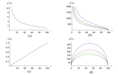
Figure 2: For the Schwarzschild black hole in massless gravity, radial solutions of the geodesic deviation equation: (a) for $\eta^{\hat{1}}(b)=1$, $\frac{d\eta^{\hat{1}}(b)}{d\tau}$=0 with $m=10$, (b) for $\eta^{\hat{1}}(b)=1$, $\frac{d\eta^{\hat{1}}(b)}{d\tau}$=1, $m=5,~{}10,~{}15,~{}20$ from bottom to top, and angular solutions of the geodesic deviation equation, (c) for $\eta^{\hat{i}}(b)=1$, $\frac{d\eta^{\hat{i}}(b)}{d\tau}$=0 with $m=10$, and (d) for $\eta^{\hat{i}}(b)=1$, $\frac{d\eta^{\hat{i}}(b)}{d\tau}$=1, $m=5,~{}10,~{}15,~{}20$ from top to bottom.

Since we are considering a body falling from rest at $r=b$ , we find the constants of integration as

$$d_{1}=\frac{b^{2}}{m}\frac{d\eta^{\hat{1}}(b)}{d\tau},~{}~{}d_{2}=\frac{m}{b^{2}}\eta^{\hat{1}}(b),~{}~{}d_{3}=\frac{1}{b}\eta^{\hat{i}}(b),~{}~{}d_{4}=-b\frac{d\eta^{\hat{i}}(b)}{d\tau}.$$ (4.9)

Thus, the solutions Crispino:2016pnv are finally written as

$$\eta^{\hat{1}}(r) = b\sqrt{\frac{2b}{m}}\frac{d\eta^{\hat{1}}(b)}{d\tau}\left(\frac{b}{r}-1\right)^{1/2}+\eta^{\hat{1}}(b)\left[\frac{3}{2}-\frac{r}{2b}+\frac{3}{4}\left(\frac{b}{r}-1\right)^{1/2}\cos^{-1}\left(\frac{2r}{b}-1\right)\right],$$ (4.10)

$$\eta^{\hat{i}}(r) = r\left[\frac{\eta^{\hat{i}}(b)}{b}+\sqrt{\frac{2b}{m}}\frac{d\eta^{\hat{i}}(b)}{d\tau}\left(\frac{b}{r}-1\right)^{1/2}\right].$$ (4.11)

These solutions of $\eta^{\hat{1}}(r)$ and $\eta^{\hat{i}}(r)$ show how the initial radial and angular separations of two nearby geodesics are changed while falling to the Schwarzschild black hole in massless gravity. It is appropriate to comment that $\eta^{\hat{1}}(b)$ and $\eta^{\hat{i}}(b)$ are initial separation distances between two nearby geodesics at $r=b$ to the radial and angular directions, respectively. Moreover, $\frac{d\eta^{\hat{1}}(b)}{d\tau}$ and $\frac{d\eta^{\hat{i}}(b)}{d\tau}$ are initial velocities at $r=b$ to the radial and angular directions, respectively, which mean either exploding when they are positive, or imploding when they are negative. Here let us consider two cases where one is $\eta^{\hat{\alpha}}(b)\neq 0$, $\frac{d\eta^{\hat{\alpha}}(b)}{d\tau}=0$ $(\alpha=1,~{}2,~{}3)$, and the other is $\eta^{\hat{\alpha}}(b)\neq 0$, $\frac{d\eta^{\hat{\alpha}}(b)}{d\tau}\neq 0$. In Fig. 2(a), (c) correspond to the former case, and (b), (d) to the latter case. Note that when $\frac{d\eta^{\hat{\alpha}}(b)}{d\tau}=0$, $\eta^{\hat{\alpha}}(r)$ become

$$\eta^{\hat{1}}(r) = \eta^{\hat{1}}(b)\left[\frac{3}{2}-\frac{r}{2b}+\frac{3}{4}\left(\frac{b}{r}-1\right)^{1/2}\cos^{-1}\left(\frac{2r}{b}-1\right)\right],$$ (4.12)

$$\eta^{\hat{i}}(r) = \frac{\eta^{\hat{i}}(b)}{b}r,$$ (4.13)

respectively, which show that the separation distance goes to infinity for the radial component due to the last term in (4.12) and goes to zero for the angular one as the body is falling to the black hole, a process known well as spaghettification.

On the other hand, when $\frac{d\eta^{\hat{\alpha}}(b)}{d\tau}\neq 0$, the radial components show the similar behaviors as in Fig. 2(b), however the separation distances of the angular components start to increase, reach a peak, then decrease to zero, as the body falls to the black hole, which is shown in Fig. 2(d). It is interesting to note that the separation distance of the angular component is smaller as the mass of the black hole is larger. Note also that by varying the initial distances of $\eta^{\hat{\alpha}}(b)$ at $r=b$, the angular component is more deformed as $\eta^{\hat{i}}(b)$ is larger.

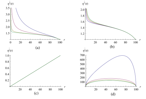
Figure 3: For the Schwarzschild black hole in holographic massive gravity, radial solutions of the geodesic deviation equation for $\eta^{\hat{1}}(b)=1$, $\frac{d\eta^{\hat{1}}(b)}{d\tau}=0$: (a) with $m=10$ by varying $R=0.001,~{}0.01,~{}0.1,~{}0.5$ from top to bottom, (b) with $R=0.1$ by varying $m=5,~{}10,~{}15,~{}20$ from bottom to top, and angular solution of the geodesic deviation equation, (c) for $\eta^{\hat{i}}(b)=1$, $\frac{d\eta^{\hat{i}}(b)}{d\tau}$=0, $m=10$ and $R=0.001,~{}0.01,~{}0.1,~{}0.5$, and (d) for $\eta^{\hat{i}}(b)=1$, $\frac{d\eta^{\hat{i}}(b)}{d\tau}$=1, and $R=0.001$ by varying $m=5,~{}10,~{}15,~{}20$ from top to bottom.

Now, inspired by the massless case, let us solve the geodesic deviation equations (4.1) and (4.2) by noting that the constant terms of ${\cal C}$ are cancelled out and thus expanding the integrand to the power of $R$ up to the $R^{4}$ terms in order to see the massive graviton effect. Then, one can integrate it out term by term as follows

$$\eta^{\hat{1}}(r) = d_{1}\sqrt{\frac{2m}{b}}\left(1+\frac{bRr}{m}\right)^{1/2}\left(\frac{b}{r}-1\right)^{1/2}$$ (4.14)

$$+ d_{2}\frac{b}{2m}\left(1+\frac{bRr}{m}\right)^{1/2}\left[2bg_{1}(r)+\frac{3b}{2}g_{2}(r)\left(\frac{b}{r}-1\right)^{1/2}\cos^{-1}\left(\frac{2r}{b}-1\right)\right],$$

$$\eta^{\hat{i}}(r) = d_{3}r-d_{4}\sqrt{\frac{2b}{m}}\frac{r}{b}\left[g_{3}(r)\left(\frac{b}{r}-1\right)^{1/2}-g_{4}(r)\cos^{-1}\left(\frac{2r}{b}-1\right)\right],$$ (4.15)

where

$$g_{1}(r) = \frac{3}{2}-\frac{r}{2b}+\left(\frac{3r^{2}}{8b}+\frac{15r}{16}-\frac{45b}{16}\right)\left(\frac{bR}{m}\right)-\left(\frac{5r^{3}}{16b}+\frac{35r^{2}}{64}+\frac{175br}{128}-\frac{525b^{2}}{128}\right)\left(\frac{bR}{m}\right)^{2}$$

$$+\left(\frac{35r^{4}}{128b}+\frac{105r^{3}}{256}+\frac{735br^{2}}{1024}+\frac{3675b^{2}r}{2048}-\frac{11025b^{3}}{2048}\right)\left(\frac{bR}{m}\right)^{3}$$

$$-\left(\frac{63r^{5}}{256b}+\frac{693r^{4}}{2048}+\frac{2079br^{3}}{4096}+\frac{14553b^{2}r^{2}}{16384}+\frac{72765b^{3}r}{32768}-\frac{218295b^{4}}{32768}\right)\left(\frac{bR}{m}\right)^{4}+{\cal O}(R^{5}),$$

$$g_{2}(r) = 1-\frac{15b}{8}\left(\frac{bR}{m}\right)+\frac{175b^{2}}{64}\left(\frac{bR}{m}\right)^{2}-\frac{3675b^{3}}{1024}\left(\frac{bR}{m}\right)^{3}+\frac{72765b^{4}}{16384}\left(\frac{bR}{m}\right)^{4}+{\cal O}(R^{5}),$$

$$g_{3}(r) = 1+\frac{3br}{16}\left(\frac{bR}{m}\right)^{2}-\left(\frac{5br^{2}}{64}+\frac{15b^{2}r}{128}\right)\left(\frac{bR}{m}\right)^{3}+\left(\frac{35br^{3}}{768}+\frac{175b^{2}r^{2}}{3072}+\frac{175b^{3}r}{2048}\right)\left(\frac{bR}{m}\right)^{4}+{\cal O}(R^{5}),$$

$$g_{4}(r) = \frac{b}{4}\left(\frac{bR}{m}\right)-\frac{3b^{2}}{32}\left(\frac{bR}{m}\right)^{2}+\frac{15b^{3}}{256}\left(\frac{bR}{m}\right)^{3}-\frac{175b^{4}}{4096}\left(\frac{bR}{m}\right)^{4}+{\cal O}(R^{5}).$$ (4.16)

Here, the constants of integration are given by

$$d_{1} = \frac{b^{2}}{m}\left(1+\frac{b^{2}R}{m}\right)^{-1}\frac{d\eta^{\hat{1}}(b)}{d\tau},~{}~{}d_{2}=\frac{m}{b^{2}}\left(1+\frac{b^{2}R}{m}\right)^{-1/2}g^{-1}_{1}(b)\eta^{\hat{1}}(b),$$

$$d_{3} = \frac{1}{b}\eta^{\hat{i}}(b),~{}~{}~{}~{}~{}~{}~{}~{}~{}~{}~{}~{}~{}~{}~{}~{}~{}~{}~{}~{}~{}~{}~{}~{}~{}d_{4}=-b\frac{d\eta^{\hat{i}}(b)}{d\tau}.$$ (4.17)

Thus, the solutions are finally written as

$$\eta^{\hat{1}}(r) = b\sqrt{\frac{2b}{m}}\left(1+\frac{b^{2}R}{m}\right)^{-1}\frac{d\eta^{\hat{1}}(b)}{d\tau}\left(1+\frac{bRr}{m}\right)^{1/2}\left(\frac{b}{r}-1\right)^{1/2}$$ (4.18)

$$+ \left(1+\frac{b^{2}R}{m}\right)^{-1/2}g^{-1}_{1}(b)\eta^{\hat{1}}(b)\left(1+\frac{bRr}{m}\right)^{1/2}\left[g_{1}(r)+\frac{3}{4}g_{2}(r)\left(\frac{b}{r}-1\right)^{1/2}\cos^{-1}\left(\frac{2r}{b}-1\right)\right],$$

$$\eta^{\hat{i}}(r) = r\left[\frac{\eta^{\hat{i}}(b)}{b}+\sqrt{\frac{2b}{m}}\frac{d\eta^{\hat{i}}(b)}{d\tau}\left(g_{3}(r)\left(\frac{b}{r}-1\right)^{1/2}-g_{4}(r)\cos^{-1}\left(\frac{2r}{b}-1\right)\right)\right].$$ (4.19)

In Fig. 3, we have drawn the radial and angular components of the separation vectors by varying $R$ and the mass of the black holes, respectively. Here, we have found that the massive gravitons keep tightening two nearby geodesics either as the graviton’s mass $\tilde{m}$ embodied in $R$ is bigger in Fig. 3(a) or as the black hole’s mass $m$ is smaller for a given $R$ in Fig. 3(b). It is also interesting to see that when $\frac{d\eta^{\hat{i}}(b)}{d\tau}=0$ the angular component is linearly shrink to be zero as the body approaches the singularity by

$$\eta^{\hat{i}}(r) = \frac{\eta^{\hat{i}}(b)}{b}r,$$ (4.20)

regardless of the black hole’s mass as shown in Fig. 3(c). Moreover, when $\frac{d\eta^{\hat{i}}(b)}{d\tau}\neq 0$ with a fixed $R$, two nearby geodesics are more easily separated as the mass of the black hole is smaller, then reach a peak, decrease to zero, as the body falls to the black hole, as seen in Fig. 3(d).

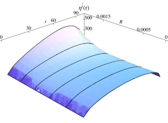
Figure 4: For the Schwarzschild black hole in holographic massive gravity, angular solution of the geodesic deviation equation by varying $R$ with $\eta^{\hat{1}}(b)=1$, $\frac{d\eta^{\hat{1}}(b)}{d\tau}=1$ and $m=10$.

In Fig. 4, we have also drawn the angular solution of the geodesic deviation equation by varying the massive graviton parameter $R$ continuously with fixed mass $m$ of the black hole. This shows that as $R$ is increased, the distance between the nearby geodesics in the angular direction is increased near the departure point of $r=b$.

V Discussion

In summary, we have studied the geodesics and tidal effects produced in the spacetime of the Schwarzschild black hole in Vegh’s holographic massive gravity, which has two additional mass parameters of $R$ and ${\cal C}$ due to the existence of massive gravitons, comparing with the known results in massless gravity. As a result, we have newly found that massive gravitons affect the angular component of the tidal force giving an additional term proportional to only $R/r$ coming from $f^{\prime}(r)$, while the radial component of the tidal force in holographic massive gravity is the same with the one in massless gravity, which is derived from $f^{\prime\prime}(r)$.

In order to see its implication, we have further investigated the solutions of the geodesic deviation equations, which show the behavior of two nearby geodesics freely falling into the Schwarzschild black hole. As for the Schwarzschild black hole in massless gravity, with boundary conditions of $\eta^{\hat{\alpha}}(b)\neq 0$ and $\frac{d\eta^{\hat{\alpha}}(b)}{d\tau}=0$, the radial component gets infinitely stretched and the angular component is compressed to zero by the tidal force as shown in Figs. 2(a) and 2(c). However, with exploding boundary conditions of $\eta^{\hat{\alpha}}(b)\neq 0$ and $\frac{d\eta^{\hat{\alpha}}(b)}{d\tau}\neq 0$, the separation distances of the angular component start to get stretched, reach a peak and then get compressed as shown in Fig. 2(d), while the radial components behave similarly to the case of $\eta^{\hat{\alpha}}(b)\neq 0$ and $\frac{d\eta^{\hat{\alpha}}(b)}{d\tau}=0$ as in Fig. 2(b).

On the other hand, as for the Schwarzschild black hole in holographic massive gravity, with boundary conditions of $\eta^{\hat{\alpha}}(b)\neq 0$ and $\frac{d\eta^{\hat{\alpha}}(b)}{d\tau}=0$, the radial components keep tightening and after passing the event horizons get abruptly infinitely stretched due to the massive gravitons, as shown in Fig. 3(a), while the angular components are unaffectedly compressed as in Fig. 3(c). With exploding boundary conditions of $\eta^{\hat{\alpha}}(b)\neq 0$ and $\frac{d\eta^{\hat{\alpha}}(b)}{d\tau}\neq 0$, the radial components also show the abrupt stretch after passing the event horizons, while the angular components are more deformed as the mass of a black hole is smaller as shown in Figs. 3(b) and 3(d). As a result, in the Schwarzschild black hole in holographic massive gravity, we have newly shown that the massive gravitons keep tightening radial components of two nearby geodesics as $R$ is bigger. Moreover, the massive gravitons make angular components of two nearby geodesics more deformed as the mass of the black holes $m$ is smaller.

Finally, it seems appropriate to comment that all known massive gravities may not be excluded by recent tests of GR in which graviton mass bounds Will:1997bb were continuously improved in GW150914 Abbott:2016blz and GW170104 Abbott:2017vtc (see also LIGOScientific:2019fpa ; 1826681 ). Therefore, it would be interesting to study more on various gravity models related with tidal effects including the one in holographic massive gravity to shed light on the nature of gravity.

- (1) T. Clifton, P. G. Ferreira, A. Padilla and C. Skordis, Phys. Rept. 513, 1 (2012) [arXiv:1106.2476 [astro-ph.CO]].
- (2) K. Hinterbichler, Rev. Mod. Phys. 84, 671 (2012) [arXiv:1105.3735 [hep-th]].
- (3) C. de Rham, Living Rev. Rel. 17, 7 (2014) [arXiv:1401.4173 [hep-th]].
- (4) M. Fierz and W. Pauli, Proc. Roy. Soc. Lond. A 173, 211 (1939).
- (5) D. G. Boulware and S. Deser, Phys. Rev. D 6, 3368 (1972).
- (6) H. van Dam and M. J. G. Veltman, Nucl. Phys. B 22, 397 (1970).
- (7) V. I. Zakharov, JETP Lett. 12, 312 (1970).
- (8) C. de Rham and G. Gabadadze, Phys. Rev. D 82, 044020 (2010) [arXiv:1007.0443 [hep-th]].
- (9) C. de Rham, G. Gabadadze and A. J. Tolley, Phys. Rev. Lett. 106, 231101 (2011) [arXiv:1011.1232 [hep-th]].
- (10) S. F. Hassan and R. A. Rosen, Phys. Rev. Lett. 108, 041101 (2012) [arXiv:1106.3344 [hep-th]].
- (11) S. F. Hassan, R. A. Rosen and A. Schmidt-May, JHEP 1202, 026 (2012) [arXiv:1109.3230 [hep-th]].
- (12) D. Vegh, arXiv:1301.0537 [hep-th].
- (13) R. A. Davison, Phys. Rev. D 88, 086003 (2013) [arXiv:1306.5792 [hep-th]].
- (14) M. Blake and D. Tong, Phys. Rev. D 88, 106004 (2013) [arXiv:1308.4970 [hep-th]].
- (15) M. Blake, D. Tong and D. Vegh, Phys. Rev. Lett. 112, 071602 (2014) [arXiv:1310.3832 [hep-th]].
- (16) R. G. Cai, Y. P. Hu, Q. Y. Pan and Y. L. Zhang, Phys. Rev. D 91, 024032 (2015) [arXiv:1409.2369 [hep-th]].
- (17) A. Adams, D. A. Roberts and O. Saremi, Phys. Rev. D 91, 046003 (2015) [arXiv:1408.6560 [hep-th]].
- (18) S. H. Hendi, S. Panahiyan and B. Eslam Panah, JHEP 1601, 129 (2016) [arXiv:1507.06563 [hep-th]].
- (19) Y. P. Hu, X. M. Wu and H. Zhang, Phys. Rev. D 95, 084002 (2017) [arXiv:1611.09042 [gr-qc]].
- (20) D. C. Zou, R. Yue and M. Zhang, Eur. Phys. J. C 77, 256 (2017) [arXiv:1612.08056 [gr-qc]].
- (21) S. H. Hendi, R. B. Mann, S. Panahiyan and B. Eslam Panah, Phys. Rev. D 95, 021501 (2017) [arXiv:1702.00432 [gr-qc]].
- (22) L. Tannukij, P. Wongjun and S. G. Ghosh, Eur. Phys. J. C 77, 846 (2017) [arXiv:1701.05332 [gr-qc]].
- (23) S. H. Hendi, B. Eslam Panah, S. Panahiyan, H. Liu and X.-H. Meng, Phys. Lett. B 781, 40 (2018) [arXiv:1707.02231 [hep-th]].
- (24) S. H. Hendi and A. Dehghani, Eur. Phys. J. C 79, 227 (2019) [arXiv:1811.01018 [gr-qc]].
- (25) M. Chabab, H. El Moumni, S. Iraoui and K. Masmar, Eur. Phys. J. C 79, 342 (2019) [arXiv:1904.03532 [hep-th]].
- (26) S. T. Hong, Y. W. Kim and Y. J. Park, Phys. Rev. D 99, 024047 (2019) [arXiv:1812.00373 [gr-qc]].
- (27) S. T. Hong, Y. W. Kim and Y. J. Park, Phys. Lett. B 800, 135116 (2020) [arXiv:1905.04860 [gr-qc]].
- (28) T. Andrade and B. Withers, JHEP 05, 101 (2014) [arXiv:1311.5157 [hep-th]].
- (29) A. Amoretti, A. Braggio, N. Maggiore, N. Magnoli and D. Musso, JHEP 1409, 160 (2014) [arXiv:1406.4134 [hep-th]].
- (30) M. Baggioli and O. Pujolas, Phys. Rev. Lett. 114, 251602 (2015) [arXiv:1411.1003 [hep-th]].
- (31) Z. Zhou, J. P. Wu and Y. Ling, JHEP 1508, 067 (2015) [arXiv:1504.00535 [hep-th]].
- (32) S. A. Hartnoll, A. Lucas and S. Sachdev, Holographic quantum matter, The MIT Press, Cambridge, 2018 [arXiv:1612.07324 [hep-th]].
- (33) L. Alberte, M. Ammon, A. Jiménez-Alba, M. Baggioli and O. Pujolàs, Phys. Rev. Lett. 120, 171602 (2018) [arXiv:1711.03100 [hep-th]].
- (34) M. Ammon, M. Baggioli and A. Jiménez-Alba, JHEP 09, 124 (2019) [arXiv:1904.05785 [hep-th]].
- (35) S. H. Hendi, G. H. Bordbar, B. Eslam Panah and S. Panahiyan, JCAP 07, 004 (2017) [arXiv:1701.01039 [gr-qc]].
- (36) C. W. Misner, K. S. Thorne and J. A. Wheeler, Gravitation, Pinceton University Press, Princeton and Oxford, 2017.
- (37) R. D’Inverno, Introducing Einstein’s Relativity, Clarendon Press, Oxford, 1992.
- (38) S. M. Carroll, Spacetime and Geometry, Addison Wesley, San Franscico, 2004.
- (39) M. P. Hobson, G. P. Efstathiou and A. N. Lasenby, General Realtivity: An Introduction for Physicists, Cambridge University Press, Cambridge, 2006.
- (40) R. Goswami and G. F. R. Ellis, [arXiv:1912.00591 [gr-qc]].
- (41) J. A. Wheeler, Mechanisms for jets, in Proceedings of a Study Week on Nuclei of Galaxies, ed. by D. J. K. O’Connell, p.539 (1971).
- (42) J. G. Hills, Nature 254, 295 (1975).
- (43) B. Carter and J. P. Luminet, Nature 296, 211 (1982).
- (44) M. J. Rees, Nature 333, 523 (1988).
- (45) S. Komossa, J. High Energy Astrophys. 7, 148 (2015).
- (46) K. Auchettl, J. Guillochon, and E. Ramirez-Ruiz, Astophys. J. 838, 149 (2017).
- (47) E. M. Rossi, N. C. Stone, J. A. P. Law-Smith, M. MacLeod, G. Lodato, J. L. Dai and I. Mandel, [arXiv:2005.12528 [astro-ph.HE]].
- (48) S. M. Mahajan, A. Qadir and V. M. Valanju, Nuovo Cim 65, 404 (1981).
- (49) M. Abdel-Megied and R. M. Gad, Chaos Solitons Fractals 23, 313-320 (2005) [arXiv:gr-qc/0402077 [gr-qc]].
- (50) L. Crispino, C.B., A. Higuchi, L. A. Oliveira and E. S. de Oliveira, Eur. Phys. J. C 76, 168 (2016) [arXiv:1602.07232 [gr-qc]].
- (51) R. M. Gad, Astrophys. Space Sci. 330, 107 (2010). [arXiv:0708.2841 [math-ph]].
- (52) M. U. Shahzad and A. Jawad, Eur. Phys. J. C 77, 372 (2017) [arXiv:1706.00281 [gr-qc]].
- (53) K. C. K. Chan and R. B. Mann, Class. Quant. Grav. 12, 1609 (1995) [arXiv:gr-qc/9501028 [gr-qc]].
- (54) K. K. Nandi, A. Bhadra, P. M. Alsing and T. B. Nayak, Int. J. Mod. Phys. D 10, 529 (2001) [arXiv:gr-qc/0008025 [gr-qc]].
- (55) V. Cardoso and P. Pani, Class. Quant. Grav. 30, 045011 (2013) [arXiv:1205.3184 [gr-qc]].
- (56) T. Harko and F. S. N. Lobo, Phys. Rev. D 86, 124034 (2012) [arXiv:1210.8044 [gr-qc]].
- (57) R. Uniyal, H. Nandan and K. D. Purohit, Mod. Phys. Lett. A 29, 1450157 (2014) [arXiv:1406.3918 [gr-qc]].
- (58) M. Sharif and S. Sadiq, J. Exp. Theor. Phys. 126, 194 (2018).
- (59) M. Sharif and L. Kousar, Commun. Theor. Phys. 69, 257 (2018)
- (60) H. C. D. Lima Junior, L. C. B. Crispino and A. Higuchi, Eur. Phys. J. Plus 135, 334 (2020) [arXiv:2003.09506 [gr-qc]].
- (61) H. C. D. L. Junior and L. Crispino, C.B., [arXiv:2005.13029 [gr-qc]].
- (62) B. P. Abbott et al. [LIGO Scientific and Virgo], Phys. Rev. Lett. 116, 061102 (2016) [arXiv:1602.03837 [gr-qc]].
- (63) B. P. Abbott et al. [LIGO Scientific and VIRGO], Phys. Rev. Lett. 118, 221101 (2017) [erratum: Phys. Rev. Lett. 121, 129901 (2018)] [arXiv:1706.01812 [gr-qc]].
- (64) M. Parikh, F. Wilczek and G. Zahariade, Int. J. Mod. Phys. D 29, 2042001 (2020) [arXiv:2005.07211 [hep-th]].
- (65) M. Parikh, F. Wilczek and G. Zahariade, [arXiv:2010.08205 [hep-th]].
- (66) M. Parikh, F. Wilczek and G. Zahariade, [arXiv:2010.08208 [hep-th]].
- (67) C. M. Will, Phys. Rev. D 57, 2061-2068 (1998) [arXiv:gr-qc/9709011 [gr-qc]].
- (68) B. P. Abbott et al. [LIGO Scientific and Virgo], Phys. Rev. D 100, 104036 (2019) [arXiv:1903.04467 [gr-qc]].
- (69) R. Abbott et al. [LIGO Scientific and Virgo], [arXiv:2010.14529 [gr-qc]].