Orbital distribution of infalling satellite halos across cosmic time

Abstract

The initial orbits of infalling subhalos largely determine the subsequent evolution of the subhalos and satellite galaxies therein and shed light on the assembly of their hosts. Using a large set of cosmological simulations of various resolutions, we quantify the orbital distribution of subhalos at infall time and its mass and redshift dependence in a large dynamic range. We further provide a unified and accurate model validated across cosmic time, which can serve as the initial condition for semi-analytic models. We find that the infall velocity $v$ follows a nearly universal distribution peaked near the host virial velocity $V_{\mathrm{h}}$ for any subhalo mass or redshift, while the infall orbit is most radially biased when $v\sim V_{\mathrm{h}}$. Moreover, subhalos that have a higher host mass or a higher sub-to-host ratio tend to move along a more radial direction with a relatively smaller angular momentum than their low host mass or low sub-to-host ratio counterparts, though they share the same normalized orbital energy. These relations are nearly independent of the redshift when using the density peak height as the proxy for host halo mass. The above trends are consistent with the scenario where the dynamical environment is relatively colder for more massive structures because their own gravity is more likely to dominate the local potentials. Based on this understanding, the more massive or isolated halos are expected to have higher velocity anisotropy.

tablenum SIXtablenum

1 Introduction

In the current hierarchical structure formation framework, dark matter halos grow through the accretion of diffuse matter and smaller halos. After infall, the subhalos will experience dynamical friction, tidal heating and stripping, and ultimately get dissolved into the hosts (see, e.g., Zavala & Frenk 2019 and references therein). Meanwhile, the inhabiting satellite galaxies might undergo morphology transformation arising from ram-pressure stripping, strangulation, harassment, and tidal shock heating; the interactions and mergers, especially major mergers, can drive the evolution of the central galaxy (Mo et al. 2010). The efficiency and the outcome of all of these processes depend critically on the details of subhalo orbits. On the other hand, the subhalos are building blocks of larger halos; their orbital distribution can help us to understand the phase-space structure of halos and the environment dependence, including the mass profile (Dalal et al., 2010), angular momentum (Vitvitska et al., 2002; Bett & Frenk, 2012; Benson et al., 2020), and velocity anisotropy (Ludlow et al., 2011; Sparre & Hansen, 2012; Shi et al., 2015). Moreover, the satellite kinematics are widely used to infer the potential of their hosts (e.g., Diaferio & Geller, 1997; More et al., 2011; Li et al., 2017, 2019) or model the galaxy clustering in redshift space (e.g., Blake et al., 2011; Zu & Weinberg, 2013; Shi et al., 2016). Therefore, the cosmological predictions for the orbital distribution of subhalos are indispensable to modeling galaxy formation, understanding halo structure, and interpreting observation.

The orbital distribution of subhalos at the time first entering their host halo are of particular interest. It represents the initial condition, which largely determines the subsequent evolution. Hence, it becomes an important ingredient of semi-analytical models (e.g., Baugh 2006; Yang et al. 2011; Jiang et al. 2020). In addition, from a practical view, the pre-merger subhalos in numerical simulations are more robust against the discrepancy among subhalo finding algorithms (Han et al. 2012, 2018; Onions et al. 2012; Behroozi et al. 2013), the artificial disruption due to insufficient resolution (Han et al., 2016; van den Bosch & Ogiya, 2018), or the baryonic process (e.g., Zhu et al. 2016; Sawala et al. 2017; Richings et al. 2020). Because these subhalos retain higher mass, reside in less dense environments, and have barely experienced the complicated dynamical interactions inside hosts compared to their evolved descendants. For this reason, semi-analytical models based on these initial conditions can outperform simulations in terms of numerical resolution, and thus become valuable complementary tools for its flexibility (Jiang et al., 2020).

In the idealized scenario of spherical collapse (Gunn & Gott 1972, see also Mo et al. 2010), assuming purely radial orbits and the conservation of energy, a mass shell first expands until reaching the turnaround radius $R_{\mathrm{ta}}$, then falls back onto the virialized halo of size $R_{\mathrm{h}}\simeq 0.5R_{\mathrm{ta}}$ and mass $M_{\mathrm{h}}$. Given $-\frac{GM_{\mathrm{h}}}{R_{\mathrm{ta}}}=-\frac{GM_{\mathrm{h}}}{R_{\mathrm{h}}}+\frac{1}{2}v^{2}$, the infalling materials (including subhalos) are expected to move radially with velocity $v\simeq\sqrt{GM_{\mathrm{h}}/R_{\mathrm{h}}}\equiv V_{\mathrm{h}}$ when they first cross the host virial radius $R_{\mathrm{h}}$. This is clearly oversimplified, because the overdensity regions are generally aspherical and perturbed by surrounding structures, which can introduce random motions.

More realistic descriptions have been studied using cosmological simulations. People find that subhalos at infall time indeed move with velocities around $V_{\mathrm{h}}$ but have intermediate orbital circularities, i.e., very radial or tangential orbits are both relatively rare (e.g., Tormen, 1997; Vitvitska et al., 2002). The subhalos tend to follow more radial orbits with smaller scaled angular momentum and pericenter distance for more massive hosts (Wetzel, 2011; Jiang et al., 2015) or higher sub-to-host mass ratio (Tormen, 1997; Wang et al., 2005; Jiang et al., 2015). Their position vectors are aligned with the shape of the hosts and with the principal axes of external tidal fields (e.g., Benson, 2005; Wang et al., 2005; Libeskind et al., 2014; Shi et al., 2015; Kang & Wang, 2015; Wang & Kang, 2018), in particular, the tangential velocity increases significantly with the strength of the tidal field (Shi et al., 2015).

An accurate depiction of the mass and redshift dependence for subhalo orbits is essential to model the halo assembly and galaxy formation across cosmic time. However, most works have focused on the host halos at $z=0$ (e.g., Wang et al. 2005; Jiang et al. 2015) or at very few time snapshots (Benson, 2005), and the limited sample size and dynamic ranges have inhibited precisely characterizing the mass and redshift dependence. Wetzel (2011) reported that the subhalo orbits become more radial at higher redshift for given halo mass, and provided fitting formulae to the orbital circularity and pericenter distance as a function of the host mass and redshift. Nevertheless, as pointed out by Jiang et al. (2015), Wetzel was unable to detect the dependence on the sub-to-host ratio and did not examine the correlation between the two orbital parameters.

In this paper, we aim to provide a comprehensive and unified description of the orbits of infalling subhalos across cosmic time. Using merging halo pairs from 16 cosmological simulations of various resolutions, the unprecedented large sample size and dynamic range allow us to characterize the joint distribution of orbital parameters and the mass and redshift dependence with high precision. While the general trend is qualitatively consistent with previous discoveries, we have much better statistics for the cases that are important but generally poorly covered in previous studies, including massive cluster halos, major mergers, or halos at high redshift. Moreover, we find a clear dependence of the infall angle on the velocity for the first time. The infall angle is most radially biased when $v\sim V_{\mathrm{h}}$, which is contrary to the assumption made by Jiang et al. (2015).

It would be convenient to have analytical formulae for orbital distribution. However, the large parameter space makes any unified description intractable, especially considering the nontrivial redshift dependence reported by Wetzel (2011). Inspired by the halo formation theory (e.g., Bardeen et al. 1986; Sheth et al. 2001; Mo et al. 2010), we find that using the peak height $\nu$ as a proxy for host mass can remove the redshift (and likely the cosmology) dependence, which hence allows us to build an accurate but simple model.

The structure of this paper is as follows. We first introduce the simulations and merging halos in Section 2. We then present our model for the orbital distribution in Section 3, and verify the model with simulation data in Section 4. We discuss the results in Section 5 and summarize in Section 6.

We adopt the host halo’s center and velocity as the reference frame for subhalo kinematics through this paper. The Hubble flow is included in subhalo velocity.

2 Data and method

2.1 Simulations and halos

This work is based on a set of high-resolution $N$-body simulations (Jing et al., 2007). It contains 16 realizations of three resolutions that were carried out with the parallel particle–particle–particle–mesh ($\rm{P^{3}M}$) code (Jing & Suto, 2002) under a flat $\Lambda\mathrm{CDM}$ cosmology with $\Omega_{\mathrm{m}}=0.268$, $\Omega_{\Lambda}=0.732$, $H_{0}=71\,\mathrm{km\,s}^{-1}\mathrm{Mpc}^{-1}$, $n_{\mathrm{s}}=1$, $\sigma_{8}=0.85$. Though the parameters are not the most up to date, our results are possibly not very sensitive to the cosmological parameters, as we argue in Section 5.2. Each realization contains $1024^{3}$ particles within periodic boundaries and outputs a series of snapshots equally spaced in $\log(a)$. The detailed parameters, including the box size, resolution, and output redshifts, are listed in Table 1. The realizations belong to three different resolutions that are labeled as L150, L300, and L600, respectively, according to the box size in units of $h^{-1}\mathrm{Mpc}$. Such a configuration not only enlarges the sample size and dynamic range greatly but also enables better discrimination of the numerical effects.

Table 1: Simulation parameters. The simulations are labeled into three groups by resolution. The columns present the label of the group, number of realizations, box size, number of particles, particle mass, softening length, the redshift range, and number of output snapshots, respectively.

Label	$N_{\mathrm{realization}}$	$L_{\mathrm{box}}$	$N_{\mathrm{p}}$	$m_{\mathrm{p}}$	$\epsilon_{\mathrm{soften}}$	$z_{\mathrm{snap}}$	$N_{\mathrm{snap}}$
		$h^{-1}\mathrm{Mpc}$		$h^{-1}M_{\odot}$	$h^{-1}\mathrm{kpc}$
L150	8	150	$1024^{3}$	$2.34\text{\times}{10}^{8}$	5	$[0.0,16.9]$	100
L300	4	300	$1024^{3}$	$1.87\text{\times}{10}^{9}$	10	$[0.0,16.9]$	100
L600	4	600	$1024^{3}$	$1.50\text{\times}{10}^{10}$	30	$[0.0,\phantom{0}7.3]$	024

For each simulation snapshot, we identify the halos using the standard Friends-of-Friends (FoF, Davis et al. 1985) algorithm with a linking length equal to $0.2$ times the mean particle separation. The center and velocity of a halo are specified by its largest subhalo (see below). The virial mass $M_{\mathrm{h}}$ and radius $R_{\mathrm{h}}$ are defined as the quantities of a spherical region enclosing the halo center with a mean density equal to $\Delta_{\text{vir}}\rho_{\mathrm{crit}}$, where $\Delta_{\text{vir}}$ is the virial factor (Bryan & Norman, 1998), and $\rho_{\mathrm{crit}}$ is the critical density of the universe at the snapshot. We characterize the halo mass across cosmic time by the peak height, $\nu(M_{\mathrm{h}},z)$, which is the natural unit in the Press & Schechter (1974) formalism (see also Bond et al. 1991, Mo et al. 2010). The peak height is defined as $\nu=\delta_{\text{col}}(z)/\sigma(M_{\mathrm{h}},z)$, where $\delta_{\text{col}}(z)=1.686\,\Omega_{m}(z)^{0.0055}$ is the critical overdensity required for spherical collapse at $z$ and $\sigma^{2}(M_{\mathrm{h}},z)$ is the variance of the density field smoothed on scale of $M_{\mathrm{h}}$ predicted by linear theory. At a given redshift, $\nu$ is a monotonic function of the halo mass (see Figure 1).

We apply the Hierarchical Bound-Tracing (HBT, Han et al. 2012) algorithm to search subhalos and build merger trees. HBT is considered to be the state of the art code for finding and tracing subhalos according to various systematical tests (Han et al., 2012, 2018; Onions et al., 2012; Srisawat et al., 2013). Unlike the conventional algorithms like SUBFIND (Springel et al., 2001) that search subhalos at individual snapshots separately, HBT identifies (sub)halos as they form, tracks their evolution as they merge, and builds their merger trees simultaneously, hence performing reliably even in the very dense background of a host halo. The mass $m$ of a subhalo is defined as its self-bound mass, while the position and velocity are defined as the average position and velocity of the most bound 25% core particles. This definition is more physical and robust than that based on the center of mass of all member particles (see Han et al. 2012 for details).

To alleviate the numerical effects, we only use the subhalos with more than 60 bound particles and halos with more than 600 particles within $R_{\mathrm{h}}$. This halo mass limit corresponds to $M_{\mathrm{h}}=$1.4\text{\times}{10}^{11}$\allowbreak h^{-1}M_{\odot}$ for L150 boxes ($\nu=0.6$ at $z=0$, $\nu=3.2$ at $z=6$) and $$9\text{\times}{10}^{12}$h^{-1}M_{\odot}$ for L600 boxes. We have confirmed that the results from simulations of different resolutions are consistent when using the above selection criteria.

2.2 Merging halo pairs

We consider the subhalos that for the first time enter their host halo, or say the halo pairs that just start to merge. More specifically, at each snapshot, we pick all merging halo pairs that satisfy the following criteria:

• The center of subhalo is located in the virial radius of the host halo at the current snapshot,

• But has not been enclosed by the virial radius of this halo at any earlier snapshot.

Searching through all snapshots of 16 simulations, we find $6.6\times 10^{6}$ such halo pairs in total, making a sample far larger than that used in previous related work.

We further use cubic splines to interpolate the subhalo orbits between adjoint snapshots to find the precise crossing time. Assuming that the halo size is evolving exponentially with time, we solve the exact redshift $z$ when the center of the subhalo reaches the virial radius and the position and velocity of subhalo, and masses of both halos at this particular moment. The details are given in the Appendix. Note that a subhalo with a higher velocity tends to be found at a position deeper in the halo, and thus shows a larger deviation from the expected distribution at infall time. The interpolation can help to reduce such artificial effects. Similar treatment has been widely considered in earlier works (e.g., Benson 2005; Jiang et al. 2015; Fillingham et al. 2015).

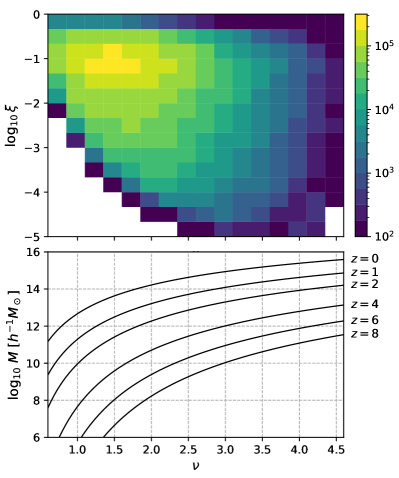
Figure 1: Number of halo pairs binned by the host halo’s peak height, $\nu$, and the sub-to-host mass ratio, $\xi=m/M_{\mathrm{h}}$. The relations between mass and $\nu$ at various $z$ are shown in the lower panel for reference.

We then characterize the masses of each merging halo pair by the dimensionless quantities, the host halo’s peak height, $\nu$, and the sub-to-host mass ratio, $\xi=m/M_{\mathrm{h}}$. As demonstrated later in Section 4.1, the subhalo orbital distribution almost does not depend on the redshift when $\nu$ and $\xi$ are controlled. Therefore, we can stack the halos at different epochs to further enlarge the sample size and dynamic range for better determining the orbital distribution and possible mass dependence. Figure 1 shows the stacked sample binned by $\nu$ and $\xi$. The number of halos is a decreasing function of $\nu$ and $\xi$ in theory. The actual distribution is truncated due to the mass limit that depends on both resolution and redshift (e.g., we can only resolve halo pairs with large $\nu$ and $\xi$ at high $z$), thus appears non-monotonic in the figure.

It is worth pointing out the difference between the two ways of searching halos that are about to merge. Here we consider the subhalos entering the host radius in a given time interval between adjoint snapshots, as they are directly related to the halo growth (see also Jiang et al. 2015). In early studies, people conventionally examine the neighboring (sub)halos within given distance interval $(R_{\mathrm{h}},R_{\mathrm{h}}+\Delta r)$ around the hosts at single snapshot (e.g., Tormen 1997; Benson 2005; Wang et al. 2005; Wetzel 2011). It is largely because the limited resolution prevents people from identifying and tracing subhalos across time. When using such scheme, one must apply a weighting to correct for the underrepresentation of satellites with larger infall velocity or more radial orbit, as they spend less time in this radial interval. Moreover, caution should be exercised when treating the major mergers (Benson, 2005). In contrast, taking advantage of merger trees, our sample naturally forms a complete census of all the accreted subhalos.

In the following, some more details about the sample are provided for interested readers. A host halo at a given snapshot might occur in our sample multiple times if it is merging with multiple subhalos simultaneously. Conversely, a subhalo might enter into different halos successively, e.g., the sub-subhalos falling into a new host along with their original host (sub)halos. The HBT algorithm has recorded the hierarchy of subhalos. In this paper, we only use the direct subhalos in our sample (85% of all infalling subhalos), considering that the sub-subhalos represent a different population due to the group preprocessing (e.g., Fujita 2004; McGee et al. 2009; Wetzel et al. 2013; Vijayaraghavan & Ricker 2013; Bahé et al. 2019). Nevertheless, we find that the inclusion of the sub-subhalos almost does not change the results of this paper.

We count all the newly accreted subhalos, though they do not necessarily stay within $R_{\mathrm{h}}$ afterward. After the first infall, a subhalo with high energy may escape as a flyby (Sales et al., 2007; Ludlow et al., 2009; Wang et al., 2009; Martin et al., 2020) or, more likely, traverse the halo radius multiple times until eventually getting trapped due to dynamical friction and mass growth of the host (Balogh et al., 2000; Mamon et al., 2004; Gill et al., 2005). For this reason, we do not exclude high-speed subhalos.

3 Model

Through systematical analysis of the sample in Section 2, we find that the following model provides a comprehensive and accurate description of the orbital parameter distribution of infalling subhalos across cosmic time. The model validation with cosmological simulations and related discussion are given in Section 4 and 5.

For a spherical potential, the orbit of a satellite halo can be specified by two independent parameters. Here we consider the infall velocity, $v$, and the angle, $\theta$, between the position vector and the velocity. The radial and tangential velocity are thus $v_{\mathrm{r}}=v\cos\theta$ and $v_{\mathrm{t}}=v\sin\theta$ respectively. As shown in Section 3.1, it is straightforward to transform from one set of orbital parameters to another.

•  The normalized velocity, $u=v/V_{\mathrm{h}}$, of infalling subhalos follows a log-normal distribution,

$$p(u)\mathop{}\!\mathrm{d}u=\frac{1}{\sqrt{2\pi}\sigma_{1}}\exp\left[{-\frac{\ln^{2}(u/\mu_{1})}{2\sigma_{1}^{2}}}\right]\frac{\mathop{}\!\mathrm{d}u}{u},$$ (1)

where $V_{\mathrm{h}}=\sqrt{GM_{\mathrm{h}}/R_{\mathrm{h}}}$ is the virial velocity of the host halo. It satisfies $\int_{0}^{\infty}p(u)\mathop{}\!\mathrm{d}u=1$ for any positive $\mu_{1}$ and $\sigma_{1}$. The median and the mode of $p(u)$ are $\mu_{1}$ and $\mu_{1}\mathrm{e}^{-\sigma_{1}^{2}}$ respectively. We find that the distribution of velocity is nearly independent of redshift or the masses of both halos.

•  The infall angle in terms of $\cos^{2}\theta=v_{\mathrm{r}}^{2}/v^{2}$ follows an exponential distribution that depends on the velocity $u$, the peak height of the host $\nu$, and the sub-to-host mass ratio $\xi$,

$$p(\cos^{2}\theta\mid u,\nu,\xi)\mathop{}\!\mathrm{d}\cos^{2}\theta=\frac{\eta}{\mathrm{e}^{\eta}-1}\exp\left({\eta\cos^{2}\theta}\right)\mathop{}\!\mathrm{d}\cos^{2}\theta,$$ (2)

where $\eta$ is a function of $u,\nu$ and $\xi$,

$$\eta=a_{0}\exp\left[-\frac{\ln^{2}(u/\mu_{2})}{2\sigma_{1}^{2}}\right]+A(u+1)+B,$$ (3)

with $A=a_{1}\nu+a_{2}\xi^{c}+a_{3}\nu\xi^{c}$ and $B=b_{1}+b_{2}\xi^{c}$. It satisfies $\int_{0}^{1}p(\cos^{2}\theta)\mathop{}\!\mathrm{d}\cos^{2}\theta=1$ for any $\eta$. We suggest taking $\eta=0$, i.e., $p(\cos^{2}\theta)=1$, if a negative value is obtained from Equation (3). Here $\cos^{2}\theta$ is used for the simplicity of its functional form, the distribution of $\theta$ then writes $p(\theta)=2\sin\theta\cos\theta p(\cos^{2}\theta)$.

A larger positive $\eta$ implies that the subhalo orbits are more radial on average. As demonstrated in Section 3.2, $\eta=0$ represents a fully isotropic motion of infalling subhalos at the halo radius.

•  The joint distribution of $u$ and $\theta$ then writes

$$p(u,\theta\mid\nu,\xi)=p(u)p(\theta\mid u,\nu,\xi).$$ (4)

Fitting the model with our halo sample, we obtain the values of the constants in Equation (1) and (3), $\mu_{1}$, $\sigma_{1}$, $\mu_{2}$, $a_{0}$, $a_{1}$, $a_{2}$, $a_{3}$, $b_{0}$, $b_{2}$, and $c$, which are listed in Table 2.

Table 2: Constants of the orbital distribution model for Equation (1) and (3).

$\mu_{1}$	$\sigma_{1}$	$\mu_{2}$	$a_{0}$	$a_{1}$	$a_{2}$	$a_{3}$	$b_{1}$	$b_{2}$	$c$
1.20	0.20	1.04	0.89	0.30	$-3.33$	0.56	$-1.44$	9.60	0.43

Remarkably, such a simple model can well describe the joint distribution of orbital parameters and the mass dependence in a large dynamic range across cosmic time. This model is much simpler than those in the literature. Most authors only provide fitting results in several mass or redshift bins separately (e.g. Benson, 2005; Wang et al., 2005; Jiang et al., 2015). Wetzel (2011) has employed up to 12 free parameters to fit the time evolution and host mass dependence, while some more would be required if further including the subhalo mass dependence and the correlation between orbital properties. The simplicity and accuracy of our model should be attributed to the use of the dimensionless variables ($\nu$ and $\xi$) motivated by halo formation theory and the appropriate separation of the physical components. It also warrants further investigation of the mechanism behind.

Noticing that the best-fit parameters in Table 2 satisfy $\mu_{1}\simeq\mathrm{e}^{4\sigma_{1}^{2}}$, hence $p(u)\simeq(\sqrt{2\pi}\sigma_{1}\mathrm{e}^{8\sigma_{1}^{2}})^{-1}u^{3}\exp[-\frac{\ln^{2}u}{2\sigma_{1}^{2}}]$. It seems not a simple coincidence (see Section 3.2) and possibly allows us to further simplify the model.

3.1 Distribution of other orbital parameters

There are various choices for the two parameters to specify an orbit in spherical potential. This paper (and, e.g., Benson 2005; Wang et al. 2005; Jiang et al. 2015) uses the velocities at infall for being simple and directly measurable. Other choices in the literature include the energy, $E$, and the angular momentum (e.g., Li et al., 2017), the radius of circular orbit for given $E$ and the orbital circularity (Tormen, 1997; van den Bosch, 2017), and the pericenter distance (or orbit semi-major axis) and the eccentricity (Benson, 2005; Wetzel, 2011). These have the advantage of depending only on the conserved quantities but require modeling the halo potential. In particular, the use of circularity is motivated by theoretical modeling to the dynamical friction (e.g., Lacey & Cole, 1993; Jiang et al., 2008). It is straightforward to derive the distribution of any orbital parameters from our $p(v,\theta)$ model through variable transformation and possibly marginalization.

For example, the joint distribution of $v_{\mathrm{r}},v_{\mathrm{t}}$ is given by

$$p(v_{\mathrm{r}},v_{\mathrm{t}})=\frac{1}{v}p(v,\theta),$$ (5)

where $\left\lvert\partial{(v_{\mathrm{r}},v_{\mathrm{t}})}/\partial{(v,\theta)}\right\rvert=v$ is used in the derivation. See Figure 7 for an illustration.

The joint distribution of the specific orbital energy, $E=\Phi_{0}+\frac{1}{2}v^{2}$ and the angular momentum, $L=rv_{\mathrm{t}}$, writes

$$p(E,L)=\frac{1}{v^{2}r\cos\theta}p(v,\theta),$$ (6)

where $\Phi_{0}=\Phi(R_{\mathrm{h}})$ is the potential energy at $r=R_{\mathrm{h}}$ and the Jacobian $\left\lvert\partial{(E,L)}/\partial{(v,\theta)}\right\rvert=v^{2}r\cos\theta$ is used. We can also derive the marginalized distribution. It is straightforward to show that $E$ follows a log-normal distribution similar to velocity,

$$p(E)=\frac{1}{\sqrt{2\pi}\sigma_{E}(E-\Phi_{0})}\exp\left\{{-\frac{\ln^{2}\left[(E-\Phi_{0})/\mu_{E}\right]}{2\sigma_{E}^{2}}}\right\},$$ (7)

where $\mu_{E}=\frac{1}{2}\mu_{1}^{2}V_{\mathrm{h}}^{2}$ and $\sigma_{E}=2\sigma_{1}$. Meanwhile, $L$ follows

$$p(L)=\int\delta(L-rv\sin\theta)p(v,\theta)\mathop{}\!\mathrm{d}v\mathop{}\!\mathrm{d}\theta=\int_{0}^{\frac{\pi}{2}}\frac{p(v^{\prime},\theta)d\theta}{r\sin\theta},$$ (8)

where $v^{\prime}=L/(r\sin\theta)$.

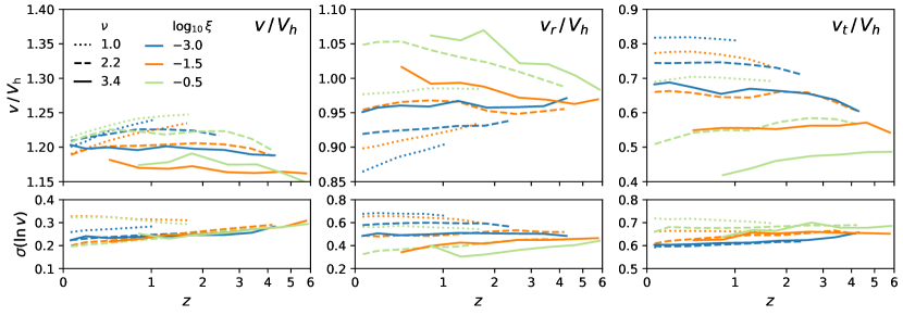
Figure 2: Dependence of subhalo infall velocity on redshift. From left to right, the top panels present the median values of $v$, $v_{\mathrm{r}}$ and $v_{\mathrm{t}}$ as functions of redshift separately. The lower panels show the dispersion of the natural logarithm of the corresponding velocities. The host mass $\nu$ and sub-to-host ratio $\xi$ used for each line are indicated by the line style and color, respectively. The velocity distribution shows no significant evolution with redshift in most cases.

3.2 Phase-space density of infalling subhalos

Here we derive the relation between the orbital distribution of accreted subhalos in given time interval and the 6D phase-space density of the infalling subhalos in radial interval near the halo radius. While the former is directly related to halo assembly as mentioned in Section 2.2, the latter is more relevant to the underlying dynamics and helpful in understanding the model in Section 3.

The phase-space density is defined as $f(\bm{r},\bm{v})=\mathop{}\!\mathrm{d}^{6}N/\mathop{}\!\mathrm{d}^{3}\bm{r}\mathop{}\!\mathrm{d}^{3}\bm{v}$. Because $f(\bm{r},\bm{v})$ only depends on $(r,v_{\mathrm{r}},v_{\mathrm{t}})$ under spherical symmetry, we can write $f(\bm{r},\bm{v})=f(r,v_{\mathrm{r}},v_{\mathrm{t}})$ or $f(r,v,\theta)$ for convenience, though $f$ still represents the 6D phase-space density (see e.g., Li et al. 2019). We only consider the distribution at the virial radius $r=R_{\mathrm{h}}$, then $f$ (as function of $\bm{v}$) actually stands for the velocity ellipsoid. Note that here $f$ represents the distribution of the subhalos at infall time, which is different from the present-day distribution. One can obtain the latter by integrating the former over the halo assembly history with necessary treatments of subhalo disruption and orbital evolution.

For fixed $v$ and $\theta$, the subhalos in a shell $r\in[R_{\mathrm{h}},R_{\mathrm{h}}+v_{\mathrm{r}}\mathop{}\!\mathrm{d}t]$ can enter the halo (and hence our sample) during the time interval $\mathop{}\!\mathrm{d}t$. The volume of the shell is then $\mathop{}\!\mathrm{d}^{3}\bm{r}=4\pi R_{\mathrm{h}}^{2}\,v\cos\theta\mathop{}\!\mathrm{d}t$. Now we can calculate the number of such infalling subhalos during $\mathop{}\!\mathrm{d}t$,

$$p(v,\theta)\mathop{}\!\mathrm{d}v\mathop{}\!\mathrm{d}\theta \propto\int_{\bm{r},\phi}f(\bm{r},\bm{v})v^{2}\sin\theta\mathop{}\!\mathrm{d}v\mathop{}\!\mathrm{d}\theta\mathop{}\!\mathrm{d}\phi\mathop{}\!\mathrm{d}^{3}\bm{r}$$

$$=8\pi^{2}R_{\mathrm{h}}^{2}\mathop{}\!\mathrm{d}t\times v^{3}\sin\theta\cos\theta f(R_{\mathrm{h}},v,\theta)\mathop{}\!\mathrm{d}v\mathop{}\!\mathrm{d}\theta$$

$$\propto v^{3}f(R_{\mathrm{h}},v,\theta)\mathop{}\!\mathrm{d}v\mathop{}\!\mathrm{d}\cos^{2}\theta.$$ (9)

So the orbital distribution of accreted subhalos, $p(v,\theta)$, differs from the phase-space distribution, $f(r\!=\!R_{\mathrm{h}},v,\theta)$, by a factor of $v^{3}\sin\theta\cos\theta$ besides the normalization.

If the subhalos move isotropically such that $f(\bm{r},\bm{v})$ is independent of $\theta$, then $\cos^{2}\theta$ of infalling subhalos follows a uniform distribution that corresponds to $\eta=0$ in Equation (2).

Moreover, it can be seen that the typical velocity of the accreted subhalos is larger than the characteristic velocity in phase space because of the factor $v^{3}$. Interestingly, solving $\mathrm{argmax}_{v,\theta}f(r\!=\!R_{\mathrm{h}},v,\theta)$ we find that the most probable velocity vector in the phase space is $v_{\mathrm{mode}}=\mu_{1}\mathrm{e}^{-4\sigma_{1}^{2}}V_{\mathrm{h}}\simeq V_{\mathrm{h}}$ and $\theta_{\mathrm{mode}}=0$ (i.e., $v_{\mathrm{r}}\simeq V_{\mathrm{h}},\ v_{\mathrm{t}}=0$), which is exactly the expectation of spherical collapse. This is clearly shown later in Figure 8.

4 Model validation

In this section, we validate the model of the subhalo initial orbital distribution using cosmological simulation data. We first examine the general trends of the mass and redshift dependence in Section 4.1, then study the detailed distribution of velocity and infall angle, respectively, in Section 4.2 and 4.3, and the joint distribution in Section 4.4. The interpretation and discussion of the results are given in Section 5.

4.1 General trends

Figure 2 shows the median and dispersion of the infall velocity, $v$, and the radial and tangential components, $v_{\mathrm{r}}$ and $v_{\mathrm{t}}$, as functions of redshift respectively. The time evolution of the median velocities is generally smaller than $5\%$ except for the major mergers of the largest halos at high $z$. For the first time, we demonstrate that the orbital distribution of infalling subhalos is nearly independent of redshift when the host peak height, $\nu$, and sub-to-host ratio, $\xi$, are controlled.

On the other hand, the orbits show apparent systematic changes with both $\nu$ and $\xi$. The mass dependence is illustrated more clearly in Figure 3, where we show the halos within the whole redshift range with better statistics. The subhalos with larger host halo or larger sub-to-host ratio have smaller $v_{\mathrm{t}}$ and slightly larger $v_{\mathrm{r}}$, hence more radial orbits, while their total velocities keep almost the same median value $\sim 1.2\ V_{\mathrm{h}}$ (with variation $\lesssim 5\%$; see also the left panel of Figure 2). Our result confirms the dependence on the mass of both halos reported previously (Tormen, 1997; Wang et al., 2005; Jiang et al., 2015) but in a larger dynamic range, especially the very massive cluster halos and major mergers that were generally poorly covered.

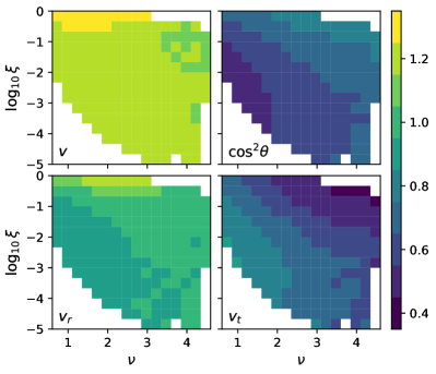
Figure 3: Orbital parameters as a function of the host mass $\nu$ and sub-to-host ratio $\xi$. The four panels show respectively the median values of $v,\ v_{\mathrm{r}}$, and $v_{\mathrm{t}}$ and the mean of $\cos^{2}\theta=v_{\mathrm{r}}^{2}/v^{2}$ for merging halos binned by $\nu$ and $\xi$. All velocities are shown in units of the host virial velocity. The subhalos with higher $\nu$ or $\xi$ are more likely to fall along the radial direction due to smaller $v_{\mathrm{t}}$, though they have a similar $v_{\mathrm{r}}$ and almost the same total velocity as their low $\nu$, $\xi$ counterparts.

Wetzel (2011) found that for halo pairs of fixed masses, $\left\langle v\right\rangle\sim 1.15V_{\mathrm{h}}$ is almost irrelevant to redshift, while $v_{\mathrm{r}}$ is larger and $v_{\mathrm{t}}$ is smaller at higher $z$. This trend is consistent with our findings, noting that $\nu$ for fixed mass is larger at higher $z$. Wetzel has also examined that picking halos with fixed $M_{\mathrm{h}}/M_{\ast}(z)$ instead of $M_{\mathrm{h}}$ at different redshifts cannot remove the redshift dependence, where $M_{\ast}(z)$ is the characteristic mass (s.t. $\nu(M_{\ast},z)=1$). He interpreted it as an intrinsic redshift dependence, which is contrary to our findings using $\nu$. The discrepancy is because the matter power spectrum of the Universe is not scale-free, so that $\nu$ is a better representative than $M/M_{\ast}$ to characterize the halo size across cosmic time.

4.2 Velocity

As shown in Figure 2, the median and the dispersion of the velocity $v$ are almost independent of redshift and mass, which implies a nearly universal distribution $p(v)$.

The independence on redshift allows us to use a larger sample by combining data at different epochs to study the mass dependence in detail. Figure 4 shows the velocity distributions of subhalos with $z<4$ in various host mass $\nu$ and sub-to-host ratio $\xi$ bins. We find that the log-normal distribution (Equation 1) presents a good description for all cases. The distribution peaks at $\mu_{1}\mathrm{e}^{-\sigma_{1}^{2}}\simeq 1.15$, which has been reported in various literature (Wetzel, 2011; Jiang et al., 2015).

However, looking closely into the figure, the data shows more extended tails than log-normal, especially for $v>1.7V_{\mathrm{h}}$. It is possible to find a more complex form to fit the long tail of the distribution. For now, we are satisfied with log-normal for its simplicity, also because the subhalos with extremely high velocity are likely to be fly-bys, thus less interesting for semi-analytical models. Nevertheless, it is worth understanding better the origin and possible influence of such high-speed subhalos in the future.

Moreover, one could find a weak mass dependence for velocity distribution. In particular, the subhalos within small host halos ($\nu=1$, dotted lines) show more extended tails at the high-velocity end ($v>2V_{\mathrm{h}}$) in Figure 4 and, consequently, have larger velocity dispersions as shown in the lower panel of Figure 2. As we argue in Section 5.1, this is likely because the environment is relatively hotter for smaller halos. Their satellites might get accelerated greatly by the external tidal field from massive neighboring clusters and large-scale structures.

There are other functional forms used to fit the velocity distribution, e.g., the Maxwell distribution (Vitvitska et al., 2002) and Voigt distribution (Jiang et al., 2015), which, however, cannot reveal the skewed tail at large $v$ as log-normal.

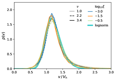
Figure 4: Infall velocity distribution for different host mass $\nu$ and sub-to-host ratio $\xi$ bins. $\nu$ and $\xi$ of each bin are indicated by the line style and color, respectively. The cyan thick solid line shows our model (Equation 1), which is a log-normal distribution.

4.3 Infall angle

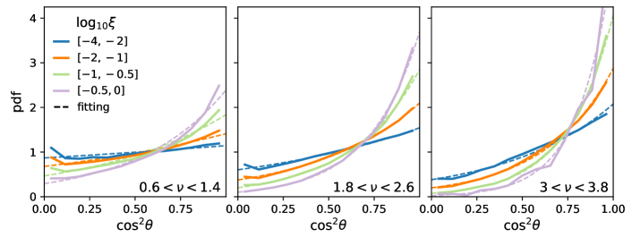
Figure 5: Distribution of the infall angle in terms of $\cos^{2}\theta$ for different host mass $\nu$ (panels) and sub-to-host ratio $\xi$ (colors) bins. The solid lines show the distributions of our halo sample, while the dashed lines represent fits of exponential function characterized by a single parameter $\eta$ (Equation 2).

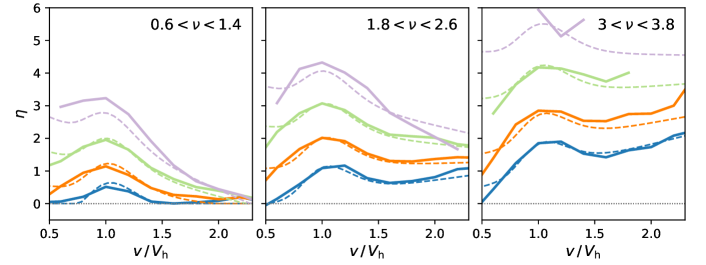
Figure 6: Distribution of infall angle as function of velocity. The distribution of angle is fully characterized by single parameter $\eta$ (Equation 2), which depends on the velocity $v$ ($x$-axis), the host mass $\nu$ (panels) and sub-to-host ratio $\xi$ (colors; see the legend of Figure 5). The solid lines show the value of $\eta$ fitted individually in each $(v,\nu,\xi)$ bin; the dashed lines show our unified model (Equation 3). Note that larger $\eta$ stands for more radial infall direction.

Figure 5 shows the distribution of the infall angle in terms of $\cos^{2}\theta=v_{\mathrm{r}}^{2}/v^{2}$ for different $\nu$ and $\xi$ bins. $\cos^{2}\theta$ can be perfectly described by the exponential function (Equation 2), $\mathop{}\!\mathrm{d}{N}/\mathop{}\!\mathrm{d}{\cos^{2}\theta}\propto\exp\left({\eta\cos^{2}\theta}\right)$. We use the relation $\left\langle\cos^{2}\theta\right\rangle=\mathrm{e}^{\eta}/(\mathrm{e}^{\eta}-1)-1/\eta$ to solve the best-fit $\eta$ from the average of $\cos^{2}\theta$ in each bin. Note that a larger $\eta$ implies that $\theta$ is smaller on average and the orbits are more radial, while $\eta=0$ represents isotropic inflow pattern (see Section 3.2). The mass dependence of the infall angle is again confirmed and consistent with the trends in Section 4.1 that $\theta$ is smaller for larger $\nu$ or $\xi$.

A complete description of the orbits comprises the velocity distribution, $p(v)$, and the conditional distribution of the falling angle for given velocity, $p(\theta|v)$. Due to the limitation of sample size in the previous work, $p(\theta|v)$ has not been investigated directly. Jiang et al. (2015) assumed that $p(\theta)$ is independent of $v$. However, they did not examine it explicitly. On the contrary, we find that $p(\theta)$ actually varies with $v$ in a non-monotonic way.

We find that the exponential function is still an excellent description for $p(\cos^{2}\theta)$ if further binning the sample by $v$, so we can use a single parameter $\eta$ as representative of $p(\cos^{2}\theta)$. Figure 6 shows $\eta$ as function of $v$. When $v$ is close to $V_{\mathrm{h}}$, the virial velocity of the host, $\eta$ reaches its maximum so that the subhalo orbits are most radially distributed. When $v$ is much smaller or larger than $V_{\mathrm{h}}$, the subhalos tend move more isotropically. Our model prediction from Equation (3) and Table 2 well captures the general trends, especially for $v\sim V_{\mathrm{h}}$.

It is worth pointing out that $\eta\geqslant 0$ for nearly all the $(v,\nu,\xi)$ bins (also justified by $\left\langle{\cos^{2}\theta}\right\rangle\geqslant 0.5$ in Figure 3), which means the radial motion is always stronger than or at least equal to the tangential one in the sense of $\left\langle v_{\mathrm{r}}^{2}/v^{2}\right\rangle\geqslant\left\langle v_{\mathrm{t}}^{2}/v^{2}\right\rangle$.

Finally, similar but non-equivalent exponential forms have been proposed to describe the angle distribution by Wang et al. (2005) and Jiang et al. (2015). Nevertheless, we find our Equation (2) provides a more accurate description to the data shown in Figure 5.

4.4 Joint distribution

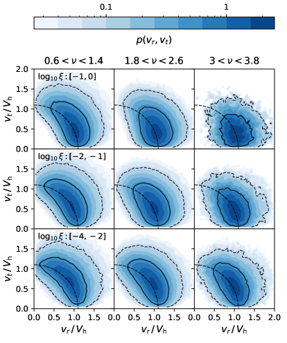
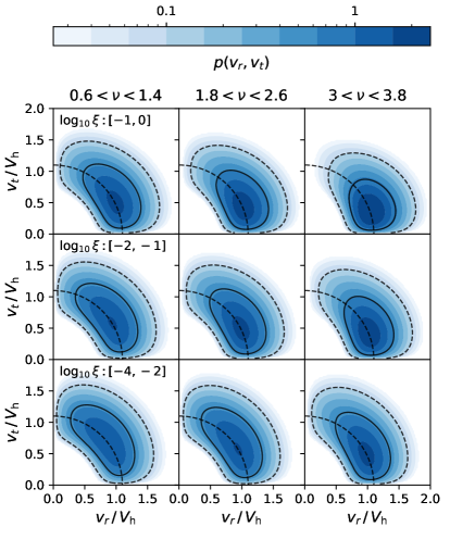
Figure 7: $p(v_{\mathrm{r}},v_{\mathrm{t}})$ of infalling subhalos (left panels) and our model prediction (right panels) for various host mass $\nu$ (columns) and sub-to-host ratio $\xi$ (rows). The colored contours show the probability density using the same color normalization. The blue solid and dashed contour lines show the 68% and 95% regions respectively, while the black dashed arcs show $v_{\mathrm{r}}^{2}+v_{\mathrm{t}}^{2}=(1.1V_{\mathrm{h}})^{2}$ for reference.

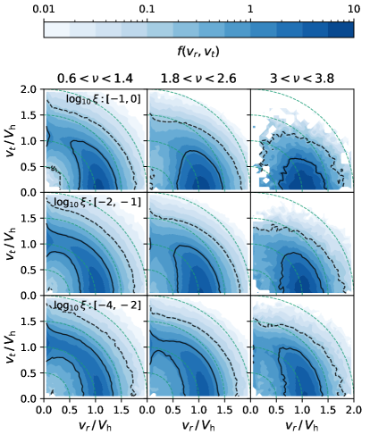
Figure 8: Similar to left panel of Figure 7, but showing the phase-space density derived in Section 3.2 for the simulation sample. The colored contours represent $f(R_{\mathrm{h}},v_{\mathrm{r}},v_{\mathrm{t}})$ as function of $v_{\mathrm{r}}$ and $v_{\mathrm{t}}$, which is actually a slice of the velocity ellipsoid. It is clear that the velocity always peaks at $V_{\mathrm{h}}$. The velocity ellipsoid approaches isotropic when $\nu$ and $\xi$ are both small.

We further demonstrate the validity of our model with the 2D velocity distribution $p(v_{\mathrm{r}},v_{\mathrm{t}})$ in Figure 7. The right panels show our model prediction using the variable transformation in Equation (5). Our model well captures the shapes of these distributions and mass dependence for various $\nu$ and $\xi$ bins. Despite the clear mass dependence, the general similarity of the velocity distributions is also notable, especially when the sub-to-host ratio is small (as for most subhalos).

Figure 8 shows the phase-space density of infalling subhalos derived in Section 3.2. The contours represent $f(R_{\mathrm{h}},\,v_{\mathrm{r}},\,v_{\mathrm{t}})$ as a function of $v_{\mathrm{r}}$ and $v_{\mathrm{t}}$, which is actually a slice of the velocity ellipsoid. The complete velocity ellipsoid, i.e., the probability density distribution in the 3D velocity space, can be obtained by rotating each panel around the $x$-axis. It is clear that the velocity ellipsoid always peaks at $v_{\mathrm{r}}\simeq V_{\mathrm{h}}$ and $v_{\mathrm{t}}=0$, which is exactly the expectation of spherical collapse. The velocity ellipsoid shows a strong radial inflow pattern when $\nu$ or $\xi$ is large, while it approaches isotropic when $\nu$ and $\xi$ are both small. Moreover, the contours also show that the phase-space distribution is more uniform along $\theta$ when $v$ is significantly larger or smaller than $V_{\mathrm{h}}$.

5 Discussion

5.1 Interpretation of results from environmental effects

The external tidal field raised from nearby objects and the large scale structure can change the velocity and moving direction of infalling subhalos, therefore, leading to deviation from the idealized radial inflow with $V_{\mathrm{h}}$ expected by spherical collapse. Consequently, halos have different accretion flow patterns in different environments (e.g., Shi et al., 2015; Kang & Wang, 2015; Wang & Kang, 2018) and hence different internal properties (Wang et al., 2011; Shi et al., 2015; Chen et al., 2016). In particular, the motions of subhalos tend to align with the tidal field’s principal axes (Shi et al., 2015). In the extreme case, if the local potential is completely dominated by the external field, the velocity ellipsoid of subhalos should be isotropic on average, because the radial direction related to the target halo is no longer special. It is exactly what we have seen for the case that $\nu$ and $\xi$ are both small in Figure 8. We believe the results reported in this paper can be understood intuitively by environmental factors as follows.

•  Mass dependence. It is obvious that the relative strength of external effects depends on the halo mass. Very massive halos generally dominate the surrounding potential field, so naturally, their satellites fall rather radially with $v\sim V_{\mathrm{h}}$. It is also consistent with the halo formation theory, that more massive halos form from more spherical overdensities with accreting matter containing less specific angular momentum (Zel’dovich, 1970; Bardeen et al., 1986; Sheth et al., 2001). Perhaps similarly, more massive subhalos are more resistant to perturbations from nearby subhalos and hence able to better keep their infalling motions. Conversely, low mass halos and low mass subhalos are more vulnerable to environmental factors that lead to a more random orbital direction and hence a larger tangential component. Interestingly, we can only observe isotropic inflow when $\nu$ and $\xi$ are both small. Even for the smallest halos in our sample, the major mergers still shows a kind of radial inflow pattern. Therefore, the dependence of $\nu$ and that of $\xi$ seem to be indeed representations of different aspects of the environment.

•  $p(v)$ and $p(\theta|v)$. The external field can either accelerate or decelerate the velocity components of a subhalo depending on its relative moving direction. Eventually, it likely affects the direction of motion more than the amplitude of velocity on average. It is probably why we find a nearly universal $p(v)$ but an angular distribution depending on mass. Nevertheless, low mass hosts indeed have slightly more subhalos with extreme velocities, as shown in Figure 4. Moreover, any significant deviation from the ideal velocity of $V_{\mathrm{h}}$ implies strong external effects typically associated with random motions. This explains the correlation between $v$ and $\theta$ that subhalos have more radial orbits when $v\sim V_{\mathrm{h}}$, and more random directions otherwise (Figure 6).

Finally, if the mass dependence is a reflection of the environmental dependence, as argued above, then it is at most a partial reflection, because halos of the same masses can reside in very different environments. For example, small halos can also dominate locally and have similarly strong radial inflow as massive halos if they are rather isolated. The final state of a halo should rely on the whole history of both mass growth and the environment.

5.2 Dependence on cosmology

As shown in Section 4.1, the subhalo orbital distribution is approximately independent of redshift when the host peak height, $\nu$, and the mass ratio, $\xi$, are controlled. Noting the dramatic changes of the cosmological parameters across cosmic time in our simulations (e.g., $\Omega_{\mathrm{m}}(z)$ evolves from $0.99$ to $0.27$ and $\sigma(8\,h^{-1}\mathrm{Mpc},z)$, the amplitude of the matter power spectrum at $8\,h^{-1}\mathrm{Mpc}$, evolves from 0.16 to 0.85 since $z=6$), it seems reasonable to speculate that our results are possibly insensitive to the cosmology, especially to the cold dark matter (CDM) cosmologies. It is because the dimensionless variables, $\nu$ and $\xi$, that are motivated by halo formation theory, present the relative rank of the halos and subhalos in a very general way. This virtue has also been justified by the approximately universal halo virial mass function (e.g., Despali et al. 2016; Diemer 2020), halo growth history (e.g., Zhao et al. 2009; van den Bosch et al. 2014), and subhalo mass function (e.g., Gao et al. 2004; Han et al. 2018) in terms of $\nu$ or $\xi$.

In other cosmologies, e.g., the warm dark matter (WDM) model, the mass function and internal structure of halos or subhalos are very different from those in CDM due to the different shape of matter power spectrum. We speculate that our results (or at least the trends) might still hold to a certain extent, because the inflow of subhalos is mainly dominated by the gravity of their host after all.

However, it is important to note that all the simulations used in this work have the same cosmology; therefore, here we are not able to justify the above arguments directly. In the future, the pertinent simulations of different cosmologies should be used to quantify the possible cosmology dependence.

6 Conclusion

In this paper, we are aiming to provide a comprehensive and unified description of the initial orbits of infalling subhalos across cosmic time. Using 16 cosmological simulations of various resolutions, the unprecedented large sample size and dynamic range allow us to characterize the joint distribution of orbital parameters and its dependence on the host mass (in terms of peak height), $\nu$ , sub-to-host mass ratio, $\xi=m/M_{\mathrm{h}}$, and redshift, $z$, with high precision.

An accurate but simple model, $p(v,\theta|\nu,\xi;z)$, is proposed (Section 3) and validated with simulations (Section 4). More specifically, we find that:

• The infall velocity, $v$, follows a nearly universal log-normal distribution (fig. 4), so does the orbital energy. The most probable velocity vector of an infalling subhalo in the phase space locates at $v_{r}\simeq V_{\mathrm{h}}$ and $v_{t}=0$ as expected by the spherical collapse model (fig. 8).

• The infall angle in terms of $\cos^{2}\theta=v_{\mathrm{r}}^{2}/v^{2}$ follows an exponential distribution that depends on $v$, $\nu$ and $\xi$ (fig. 5). The orbits are most radially biased when $v\sim V_{\mathrm{h}}$ (fig. 6).

• Subhalos with higher host mass, $\nu$, or higher sub-to-host ratio, $\xi$, have more radial orbits with relatively smaller angular momentum or pericenter distance (fig. 3). Subhalos tend to move isotropically when $\nu$ and $\xi$ are both small (fig. 8).

• The above description is nearly independent of redshift (fig. 2) and possibly insensitive to cosmology (sec. 5.2).

• It is consistent with the scenario where the dynamical environment is relatively colder for massive structures because their gravity more likely dominates the local potential (sec. 5.1).

• The approximately universal velocity distribution and the mass-dependent angle distribution seem to imply that the external tidal fields generally affect the direction rather than the amplitude of subhalo velocity on average.

We have confirmed the mass dependence of subhalo orbits reported in the literature (see Section 1) in a much larger dynamic range with better statistics. More importantly, we have proposed a unified quantitative description validated across cosmic time.

Note that our data cover $0.6\leq\nu\lesssim 4.5$ (corresponding to $10^{11.2\sim 15.6}h^{-1}M_{\odot}$ at $z=0$ and $10^{1.7\sim 12.2}h^{-1}M_{\odot}$ at $z=6$; see Figure 1), $10^{-5}\lesssim\xi\leq 1$, and $0\leq z\lesssim 6$; it is remarkable that a simple model can well characterize the orbital distribution for such wide parameter space. The simplicity and accuracy of our model could be attributed to the use of the dimensionless variables ($\nu$ and $\xi$) motivated by halo formation theory and the appropriate separation of the physical components. It warrants further investigation of the mechanism behind. In addition, future work should examine the model in a larger dynamical range (especially the halos of $\nu<0.6$) and quantify the possible cosmology dependence with pertinent simulations.

Our model can be used as the initial condition in semi-analytic models of galaxy formation (e.g., Yang et al. 2011; Jiang et al. 2020; S. Green et al. in prep. 2020) along with the halo growth history (Zhao et al., 2009) and subhalo mass function (e.g., Gao et al. 2004; Han et al. 2018) and accretion rate (e.g., Lacey & Cole 1993; Yang et al. 2011; Fakhouri et al. 2010; F.Y. Dong et al. in prep.). It also enables a better understanding of the halo structures and their dependence on environments. For example, more massive halos are expected to have higher velocity anisotropy (see, e.g., Lemze et al. 2012), so are the isolated halos. Moreover, the final dynamical state of a halo should depend on the whole history considering that $\nu$ can change with time and result in different accretion patterns.

Besides the mass dependence discussed above, we have to emphasize the general similarity in subhalo infall pattern across cosmic time, especially when the sub-to-host ratio is small (as for most of the subhalos and probably the diffuse matter). Subhalos are the building blocks of halos; therefore, this similarity in initial kinematics and the universal subhalo mass function might eventually help to understand the many reported universal self-similar halo properties, e.g., the density profile (Navarro et al., 1996, 2004), pseudo-phase-space profile (Taylor & Navarro, 2001; Navarro et al., 2010), angular momentum distribution (White, 1984; Bullock et al., 2001), and the subhalo spatial distribution (Gao et al., 2004; Springel et al., 2008; Jiang & van den Bosch, 2017; Han et al., 2016) and kinematics (Li et al., 2017, 2019).

Finally, we have only considered the average subhalo orbital distribution under the spherical symmetry in this work. A more comprehensive description of subhalo kinematics can further integrate the group infall and anisotropic accretion of subhalos (e.g., Benson, 2005; Libeskind et al., 2014; Shi et al., 2015; Kang & Wang, 2015; Shao et al., 2018), which are crucial for understanding the alignment among the halo shape, spin, and the large-scale structure (e.g., Wang et al., 2011; Chen et al., 2016; Wang & Kang, 2018; Morinaga & Ishiyama, 2020) and interpreting the anisotropic distribution of satellite galaxies reported in observations (e.g., Kroupa et al., 2005; Yang et al., 2006; Pawlowski et al., 2012; Ibata et al., 2013; Wang et al., 2020).

We are very grateful to Chunyan Jiang, Fangzhou Jiang, Xianguang Meng, Houjun Mo, Yongzhong Qian, Feng Shi, Jingjing Shi, and Xiaohu Yang for their helpful discussions, and to Frank C. van den Bosch, Sheridan B. Green, and Peng Wang for careful reading of the manuscript and insightful comments. We also thank the anonymous referee for constructive criticisms and helpful suggestions. This work is supported by NSFC (11222325, 11533006, 11621303, 11873038, 11890691, 11973032), the Knowledge Innovation Program of CAS (KJCX2-EW-J01), Shanghai talent development funding (2011069), National Key Basic Research and Development Program of China (No. 2018YFA0404504), and the 111 project (No. B20019). We gratefully acknowledge the support of the Key Laboratory for Particle Physics, Astrophysics and Cosmology, Ministry of Education.

This work made use of the High Performance Computing Resource in the Core Facility for Advanced Research Computing at Shanghai Astronomical Observatory.

Software: HBT subhalo finder and tree maker (Han et al., 2012), Colossus (Diemer, 2018), Astropy (Astropy Collaboration et al., 2013), Numpy (van der Walt et al., 2011), Scipy (Oliphant, 2007), Matplotlib (Hunter, 2007)

Appendix A Orbit Interpolation

We use the cubic spline to interpolate the subhalo orbits between adjoint snapshots to find the precise crossing time. Cubic splines are smooth curves with continuous second-order derivative (aka the acceleration). Specifically, each component of the position and velocity $\{x_{i},v_{i}\}_{i=1,2,3}$ is interpolated separately by the following equation:

$$x_{i}(t)= a_{i0}+a_{i1}t+a_{i2}t^{2}+a_{i3}t^{3},$$ (A1)

$$v_{i}(t)= a_{i1}+2a_{i2}t+3a_{i3}t^{2}.$$

The 12 unknowns, $\{a_{ij}\}$, are determined by substituting $x_{i}$ and $v_{i}$ at adjoint snapshots. We approximate the halo growth by an exponential function of time between the snapshots, $\ln R_{\mathrm{h}}(t)=b_{0}+b_{1}t$, then solve the exact infall time $t_{\mathrm{inf}}$ that satisfies $\left\lvert\bm{x}(t)\right\rvert=R_{\mathrm{h}}(t)$ and calculate corresponding $\bm{x}(t_{\mathrm{inf}}),\bm{v}(t_{\mathrm{inf}})$. Similarly, we interpolate the masses of both halos exponentially to the infall time.

References

- Astropy Collaboration et al. (2013) Astropy Collaboration, Robitaille, T. P., Tollerud, E. J., et al. 2013, A&A, 558, A33
- Bahé et al. (2019) Bahé, Y. M., Schaye, J., Barnes, D. J., et al. 2019, MNRAS, 485, 2287
- Balogh et al. (2000) Balogh, M. L., Navarro, J. F., & Morris, S. L. 2000, ApJ, 540, 113
- Bardeen et al. (1986) Bardeen, J. M., Bond, J. R., Kaiser, N., & Szalay, A. S. 1986, ApJ, 304, 15
- Baugh (2006) Baugh, C. M. 2006, RPPh, 69, 3101
- Behroozi et al. (2013) Behroozi, P. S., Wechsler, R. H., & Wu, H.-Y. 2013, ApJ, 762, 109
- Benson et al. (2020) Benson, A., Behrens, C., & Lu, Y. 2020, MNRAS, 496, 3371
- Benson (2005) Benson, A. J. 2005, MNRAS, 358, 551
- Bett & Frenk (2012) Bett, P. E., & Frenk, C. S. 2012, MNRAS, 420, 3324
- Blake et al. (2011) Blake, C., Brough, S., Colless, M., et al. 2011, MNRAS, 415, 2876
- Bond et al. (1991) Bond, J. R., Cole, S., Efstathiou, G., & Kaiser, N. 1991, ApJ, 379, 440
- Bryan & Norman (1998) Bryan, G. L., & Norman, M. L. 1998, ApJ, 495, 80
- Bullock et al. (2001) Bullock, J. S., Dekel, A., Kolatt, T. S., et al. 2001, ApJ, 555, 240
- Chen et al. (2016) Chen, S., Wang, H., Mo, H. J., & Shi, J. 2016, ApJ, 825, 49
- Dalal et al. (2010) Dalal, N., Lithwick, Y., & Kuhlen, M. 2010, arXiv:1010.2539
- Davis et al. (1985) Davis, M., Efstathiou, G., Frenk, C. S., & White, S. D. M. 1985, ApJ, 292, 371
- Despali et al. (2016) Despali, G., Giocoli, C., Angulo, R. E., et al. 2016, MNRAS, 456, 2486
- Diaferio & Geller (1997) Diaferio, A., & Geller, M. J. 1997, ApJ, 481, 633
- Diemer (2018) Diemer, B. 2018, ApJS, 239, 35
- Diemer (2020) —. 2020, ApJ, 903, 87
- Fakhouri et al. (2010) Fakhouri, O., Ma, C.-P., & Boylan-Kolchin, M. 2010, MNRAS, 406, 2267
- Fillingham et al. (2015) Fillingham, S. P., Cooper, M. C., Wheeler, C., et al. 2015, MNRAS, 454, 2039
- Fujita (2004) Fujita, Y. 2004, PASJ, 56, 29
- Gao et al. (2004) Gao, L., White, S. D. M., Jenkins, A., Stoehr, F., & Springel, V. 2004, MNRAS, 355, 819
- Gill et al. (2005) Gill, S. P. D., Knebe, A., & Gibson, B. K. 2005, MNRAS, 356, 1327
- Gunn & Gott (1972) Gunn, J. E., & Gott, J. Richard, I. 1972, ApJ, 176, 1
- Han et al. (2018) Han, J., Cole, S., Frenk, C. S., Benitez-Llambay, A., & Helly, J. 2018, MNRAS, 474, 604
- Han et al. (2016) Han, J., Cole, S., Frenk, C. S., & Jing, Y. 2016, MNRAS, 457, 1208
- Han et al. (2012) Han, J., Jing, Y. P., Wang, H., & Wang, W. 2012, MNRAS, 427, 2437
- Hunter (2007) Hunter, J. D. 2007, CSE, 9, 90
- Ibata et al. (2013) Ibata, R. A., Lewis, G. F., Conn, A. R., et al. 2013, Nature, 493, 62
- Jiang et al. (2008) Jiang, C. Y., Jing, Y. P., Faltenbacher, A., Lin, W. P., & Li, C. 2008, ApJ, 675, 1095
- Jiang et al. (2020) Jiang, F., Dekel, A., Freundlich, J., et al. 2020, arXiv:2005.05974
- Jiang & van den Bosch (2017) Jiang, F., & van den Bosch, F. C. 2017, MNRAS, 472, 657
- Jiang et al. (2015) Jiang, L., Cole, S., Sawala, T., & Frenk, C. S. 2015, MNRAS, 448, 1674
- Jing & Suto (2002) Jing, Y. P., & Suto, Y. 2002, ApJ, 574, 538
- Jing et al. (2007) Jing, Y. P., Suto, Y., & Mo, H. J. 2007, ApJ, 657, 664
- Kang & Wang (2015) Kang, X., & Wang, P. 2015, ApJ, 813, 6
- Kroupa et al. (2005) Kroupa, P., Theis, C., & Boily, C. M. 2005, A&A, 431, 517
- Lacey & Cole (1993) Lacey, C., & Cole, S. 1993, MNRAS, 262, 627
- Lemze et al. (2012) Lemze, D., Wagner, R., Rephaeli, Y., et al. 2012, ApJ, 752, 141
- Li et al. (2017) Li, Z.-Z., Jing, Y. P., Qian, Y.-Z., Yuan, Z., & Zhao, D.-H. 2017, ApJ, 850, 116
- Li et al. (2019) Li, Z.-Z., Qian, Y.-Z., Han, J., Wang, W., & Jing, Y. P. 2019, ApJ, 886, 69
- Libeskind et al. (2014) Libeskind, N. I., Knebe, A., Hoffman, Y., & Gottlöber, S. 2014, MNRAS, 443, 1274
- Ludlow et al. (2009) Ludlow, A. D., Navarro, J. F., Springel, V., et al. 2009, ApJ, 692, 931
- Ludlow et al. (2011) Ludlow, A. D., Navarro, J. F., White, S. D. M., et al. 2011, MNRAS, 415, 3895
- Mamon et al. (2004) Mamon, G. A., Sanchis, T., Salvador-Solé, E., & Solanes, J. M. 2004, A&A, 414, 445
- Martin et al. (2020) Martin, G., Jackson, R. A., Kaviraj, S., et al. 2020, MNRAS in press, arXiv:2007.07913
- McGee et al. (2009) McGee, S. L., Balogh, M. L., Bower, R. G., Font, A. S., & McCarthy, I. G. 2009, MNRAS, 400, 937
- Mo et al. (2010) Mo, H., van den Bosch, F., & White, S. 2010, Galaxy Formation and Evolution (Cambridge University Press)
- More et al. (2011) More, S., Kravtsov, A. V., Dalal, N., & Gottlöber, S. 2011, ApJS, 195, 4
- Morinaga & Ishiyama (2020) Morinaga, Y., & Ishiyama, T. 2020, MNRAS, 495, 502
- Navarro et al. (1996) Navarro, J. F., Frenk, C. S., & White, S. D. M. 1996, ApJ, 462, 563
- Navarro et al. (2004) Navarro, J. F., Hayashi, E., Power, C., et al. 2004, MNRAS, 349, 1039
- Navarro et al. (2010) Navarro, J. F., Ludlow, A., Springel, V., et al. 2010, MNRAS, 402, 21
- Oliphant (2007) Oliphant, T. E. 2007, CSE, 9, 10
- Onions et al. (2012) Onions, J., Knebe, A., Pearce, F. R., et al. 2012, MNRAS, 423, 1200
- Pawlowski et al. (2012) Pawlowski, M. S., Pflamm-Altenburg, J., & Kroupa, P. 2012, MNRAS, 423, 1109
- Press & Schechter (1974) Press, W. H., & Schechter, P. 1974, ApJ, 187, 425
- Richings et al. (2020) Richings, J., Frenk, C., Jenkins, A., et al. 2020, MNRAS, 492, 5780
- Sales et al. (2007) Sales, L. V., Navarro, J. F., Abadi, M. G., & Steinmetz, M. 2007, MNRAS, 379, 1475
- Sawala et al. (2017) Sawala, T., Pihajoki, P., Johansson, P. H., et al. 2017, MNRAS, 467, 4383
- Shao et al. (2018) Shao, S., Cautun, M., Frenk, C. S., et al. 2018, MNRAS, 476, 1796
- Sheth et al. (2001) Sheth, R. K., Mo, H. J., & Tormen, G. 2001, MNRAS, 323, 1
- Shi et al. (2016) Shi, F., Yang, X., Wang, H., et al. 2016, ApJ, 833, 241
- Shi et al. (2015) Shi, J., Wang, H., & Mo, H. J. 2015, ApJ, 807, 37
- Sparre & Hansen (2012) Sparre, M., & Hansen, S. H. 2012, J. Cosmology Astropart. Phys, 2012, 042
- Springel et al. (2001) Springel, V., White, S. D. M., Tormen, G., & Kauffmann, G. 2001, MNRAS, 328, 726
- Springel et al. (2008) Springel, V., Wang, J., Vogelsberger, M., et al. 2008, MNRAS, 391, 1685
- Srisawat et al. (2013) Srisawat, C., Knebe, A., Pearce, F. R., et al. 2013, MNRAS, 436, 150
- Taylor & Navarro (2001) Taylor, J. E., & Navarro, J. F. 2001, ApJ, 563, 483
- Tormen (1997) Tormen, G. 1997, MNRAS, 290, 411
- van den Bosch (2017) van den Bosch, F. C. 2017, MNRAS, 468, 885
- van den Bosch et al. (2014) van den Bosch, F. C., Jiang, F., Hearin, A., et al. 2014, MNRAS, 445, 1713
- van den Bosch & Ogiya (2018) van den Bosch, F. C., & Ogiya, G. 2018, MNRAS, 475, 4066
- van der Walt et al. (2011) van der Walt, S., Colbert, S. C., & Varoquaux, G. 2011, CSE, 13, 22
- Vijayaraghavan & Ricker (2013) Vijayaraghavan, R., & Ricker, P. M. 2013, MNRAS, 435, 2713
- Vitvitska et al. (2002) Vitvitska, M., Klypin, A. A., Kravtsov, A. V., et al. 2002, ApJ, 581, 799
- Wang et al. (2009) Wang, H., Mo, H. J., & Jing, Y. P. 2009, MNRAS, 396, 2249
- Wang et al. (2011) Wang, H., Mo, H. J., Jing, Y. P., Yang, X., & Wang, Y. 2011, MNRAS, 413, 1973
- Wang et al. (2005) Wang, H. Y., Jing, Y. P., Mao, S., & Kang, X. 2005, MNRAS, 364, 424
- Wang & Kang (2018) Wang, P., & Kang, X. 2018, MNRAS, 473, 1562
- Wang et al. (2020) Wang, P., Libeskind, N. I., Tempel, E., et al. 2020, ApJ, 900, 129
- Wetzel (2011) Wetzel, A. R. 2011, MNRAS, 412, 49
- Wetzel et al. (2013) Wetzel, A. R., Tinker, J. L., Conroy, C., & van den Bosch, F. C. 2013, MNRAS, 432, 336
- White (1984) White, S. D. M. 1984, ApJ, 286, 38
- Yang et al. (2011) Yang, X., Mo, H. J., Zhang, Y., & van den Bosch, F. C. 2011, ApJ, 741, 13
- Yang et al. (2006) Yang, X., van den Bosch, F. C., Mo, H. J., et al. 2006, MNRAS, 369, 1293
- Zavala & Frenk (2019) Zavala, J., & Frenk, C. S. 2019, Galax, 7, 81
- Zel’dovich (1970) Zel’dovich, Y. B. 1970, A&A, 5, 84
- Zhao et al. (2009) Zhao, D. H., Jing, Y. P., Mo, H. J., & Börner, G. 2009, ApJ, 707, 354
- Zhu et al. (2016) Zhu, Q., Marinacci, F., Maji, M., et al. 2016, MNRAS, 458, 1559
- Zu & Weinberg (2013) Zu, Y., & Weinberg, D. H. 2013, MNRAS, 431, 3319