Network Architecture Search for Domain Adaptation

Abstract

Deep networks have been used to learn transferable representations for domain adaptation. Existing deep domain adaptation methods systematically employ popular hand-crafted networks designed specifically for image-classification tasks, leading to sub-optimal domain adaptation performance. In this paper, we present Neural Architecture Search for Domain Adaptation (NASDA), a principle framework that leverages differentiable neural architecture search to derive the optimal network architecture for domain adaptation task. NASDA is designed with two novel training strategies: neural architecture search with multi-kernel Maximum Mean Discrepancy to derive the optimal architecture, and adversarial training between a feature generator and a batch of classifiers to consolidate the feature generator. We demonstrate experimentally that NASDA leads to state-of-the-art performance on several domain adaptation benchmarks.

1 Introduction

Supervised machine learning models ($\Phi$) aim to minimize the empirical test error ($\epsilon(\Phi(\mathbf{x}),\mathbf{y})$) by optimizing $\Phi$ on training data ($\mathbf{x}$) and ground truth labels ($\mathbf{y}$), assuming that the training and testing data are sampled i.i.d from the same distribution. While in practical, the training and testing data are typically collected from related domains under different distributions, a phenomenon known as domain shift (or domain discrepancy) datashift_book2009 . To avoid the cost of annotating each new test data, Unsupervised Domain Adaptation (UDA) tackles domain shift by transferring the knowledge learned from a rich-labeled source domain ($P(\mathbf{x}^{s},\mathbf{y}^{s})$) to the unlabeled target domain ($Q(\mathbf{x}^{t})$). Recently unsupervised domain adaptation research has achieved significant progress with techniques like discrepancy alignment JAN ; ddc ; ghifary2014domain ; peng2017synthetic ; long2015 ; SunS16a , adversarial alignment xu2019adversarial ; cogan ; adda ; ufdn ; DANN ; MCD_2018 ; long2018NIPS_CDAN , and reconstruction-based alignment yi2017dualgan ; CycleGAN2017 ; hoffman2017cycada ; kim2017learning . While such models typically learn feature mapping from one domain ($\Phi(\mathbf{x}^{s})$) to another ($\Phi(\mathbf{x}^{t})$) or derive a joint representation across domains ($\Phi(\mathbf{x}^{s})\otimes\Phi(\mathbf{x}^{t})$), the developed models have limited capacities in deriving an optimal neural architecture specific for domain transfer.

To advance network designs, neural architecture search (NAS) automates the net architecture engineering process by reinforcement supervision zoph2016neural or through neuro-evlolution Real2019AgingEF . Conventional NAS models aim to derive neural architecture $\alpha$ along with the network parameters $w$, by solving a bilevel optimization problem anandalingam1992hierarchical : $\Phi_{\alpha,w}=\operatorname*{arg\,min}_{\alpha}\mathcal{L}_{val}(w^{*}(\alpha),\alpha)$ $\text{s.t. }w^{*}(\alpha)=\mathrm{argmin}_{w}\mathcal{L}_{train}(w,\alpha)$, where $\mathcal{L}_{train}$ and $\mathcal{L}_{val}$ indicate the training and validation loss, respectively. While recent works demonstrate competitive performance on tasks such as image classification zoph2018learning ; liu2017hierarchical ; liu2018progressive ; real2019regularized and object detection zoph2016neural , designs of existing NAS algorithms typically assume that the training and testing domain are sampled from the same distribution, neglecting the scenario where two data domains or multiple feature distributions are of interest.

To efficiently devise a neural architecture across different data domains, we propose a novel learning task called NASDA (Neural Architecture Search for Domain Adaptation). The ultimate goal of NASDA is to minimize the validation loss of the target domain ($\mathcal{L}_{val}^{t}$). We postulate that a solution to NASDA should not only minimize validation loss of the source domain ($\mathcal{L}_{val}^{s}$), but should also reduce the domain gap between the source and target. To this end, we propose a new NAS learning schema:

$$\Phi_{\alpha,w}=\mathrm{argmin}_{\alpha}\mathcal{L}^{s}_{val}(w^{*}(\alpha),\alpha)+\mathrm{disc}(\Phi^{*}(\mathbf{x}^{s}),\Phi^{*}(\mathbf{x}^{t}))$$ (1)

$$\text{s.t.}\quad w^{*}(\alpha)=\mathrm{argmin}_{w}\enskip\mathcal{L}_{train}^{s}(w,\alpha)$$ (2)

where $\Phi^{*}=\Phi_{\alpha,w^{*}(\alpha)}$, and $\mathrm{disc}(\Phi^{*}(\mathbf{x}^{s}),\Phi^{*}(\mathbf{x}^{t}))$ denotes the domain discrepancy between the source and target. Note that in unsupervised domain adaptation, $\mathcal{L}_{train}^{t}$ and $\mathcal{L}_{val}^{t}$ cannot be computed directly due to the lack of label in the target domain.

Inspired by the past works in NAS and unsupervised domain adaptation, we propose in this paper an instantiated NASDA model, which comprises of two training phases, as shown in Figure 1. The first is the neural architecture searching phase, aiming to derive an optimal neural architecture ($\alpha^{*}$), following the learning schema of equation (1)(2). Inspired by Differentiable ARchiTecture Search (DARTS) darts , we relax the search space to be continuous so that $\alpha$ can be optimized with respect to $\mathcal{L}^{s}_{val}$ and $\mathrm{disc}(\Phi(\mathbf{x}^{s}),\Phi(\mathbf{x}^{t}))$ by gradient descent. Specifically, we enhance the feature transferability by embedding the hidden representations of the task-specific layers to a reproducing kernel Hilbert space where the mean embeddings can be explicitly matched by minimizing $\mathrm{disc}(\Phi(\mathbf{x}^{s}),\Phi(\mathbf{x}^{t}))$. We use multi-kernel Maximum Mean Discrepancy (MK-MMD) gretton2007kernel to evaluate the domain discrepancy.

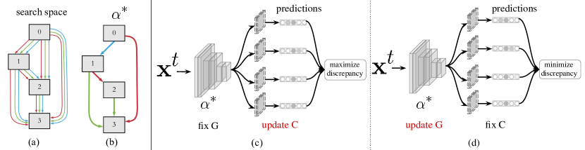
Figure 1: An overview of NASDA: (a) Continuous relaxation of the research space by placing a mixture of the candidate operations on each edge. (b) Inducing the final architecture by joint optimization of the neural architecture parameters $\alpha$ and network weights $w$, supervised by minimizing the validation loss on the source domain and reducing the domain discrepancy. (c)(d) Adversarial training of the derive feature generator $G$ and classifiers $C$.

The second training phase aims to learn a good feature generator with task-specific loss, based on the derived $\alpha^{*}$ from the first phase. To establish this goal, we use the derived deep neural network ($\Phi_{\alpha^{*}}$) as the feature generator ($G$) and devise an adversarial training process between $G$ and a batch of classifiers $C$. The high-level intuition is to first diversify $C$ in the training process, and train $G$ to generate features such that the diversified $C$ can have similar outputs. The training process is similar to Maximum Classifier Discrepancy framework (MCD) MCD_2018 except that we extend the dual-classifier in MCD to an ensembling of multiple classifiers. Experiments on standard UDA benchmarks demonstrate the effectiveness of our derived NASDA model in achieving significant improvements over state-of-the-art methods.

Our contributions of this paper are highlighted as follows:

• We formulate a novel dual-objective task of Neural Architecture Search for Domain Adaptation (NASDA), which optimize neural architecture for unsupervised domain adaptation, concerning both source performance objective and transfer learning objective.

• We propose an instantiated NASDA model that comprises two training stages, aiming to derive optimal architecture parameters $\alpha^{*}$ and feature extractor $G$, respectively. We are the first to show the effectiveness of MK-MMD in NAS process specified for domain adaptation.

• Extensive experiments on multiple cross-domain recognition tasks demonstrate that NASDA achieves significant improvements over traditional unsupervised domain adaptation models as well as state-of-the-art NAS-based methods.

2 Related Work

Deep convolutional neural network has been dominating image recognition task. In recent years, many handcrafted architectures have been proposed, including VGG vgg , ResNet resnet , Inception szegedy2015going , etc., all of which verifies the importance of human expertise in network design. Our work bridges domain adaptation and the emerging field of neural architecture search (NAS), a process of automating architecture engineering technique.

Neural Architecture Search Neural Architecture Search has become the mainstream approach to discover efficient and powerful network structures zoph2016neural ; zoph2018learning ; liu2017hierarchical ; liu2018progressive ; real2019regularized . The automatically searched architectures have achieved highly competitive performance in tasks such as image classification zoph2016neural ; zoph2018learning ; liu2017hierarchical ; liu2018progressive ; real2019regularized , object detection zoph2018learning , and semantic segmentation nas_chen2018searching . Reinforce learning based NAS methods zoph2016neural ; tan2019mnasnet ; EfficientNet are usually computational intensive, thus hampering its usage with limited computational budget. To accelerate the search procedure, many techniques has been proposed and they mainly follow four directions: (1) estimating the actual performance with lower fidelities. Such lower fidelities include shorter training times zoph2018learning ; zela2018towards training on a subset of the data pmlr-v54-klein17a , on lower-resolution images chrabaszcz2017downsampled , or with less filters per layer and less cells zoph2018learning ; Real2019AgingEF . (2) estimating the performance based on the learning curve extrapolation. Rawal et al domhan2015speeding propose to extrapolate initial learning curves and terminate those predicted to perform poorly and several papers  swersky2014freeze ; klein2016learning ; rawal2018nodes ; baker2017accelerating also leverage architectural hyperparameters to predict which partial learning curves are most promising. (3) initializing the novel architectures based on other well-trained architectures. Wei et al wei2016network introduce network morphisms to modify an architecture without changing the network objects, resulting in methods that only require a few GPU days elsken2017simple ; cai2018efficient ; jin2019auto ; cai2018path . (4) one-shot architecture search. One-shot NAS treats all architectures as different subgraphs of a supergraph and shares weights between architectures that have edges of this supergraph in common saxena2016convolutional ; brock2017smash ; pham2018efficient ; liu2018darts ; bender2019understanding ; cai2018proxylessnas ; xie2018snas . ENAS ENAS learns a RNN controller that samples architectures from the search space and trains the one-shot model using the approximate gradients. DARTS darts places a mixture of candidate operations on each edge of the one-shot model and optimizes the weights of the candidate operations with a continuous relaxation of the search space. Inspired by DARTS darts , our model employs differentiable architecture search to derive the optimal feature extractor for unsupervised domain adaptation.

Domain Adaptation Unsupervised domain adaptation (UDA) aims to transfer the knowledge learned from one or more labeled source domains to an unlabeled target domain. Various methods have been proposed, including discrepancy-based UDA approaches JAN ; ddc ; ghifary2014domain ; peng2017synthetic , adversary-based approaches cogan ; adda ; ufdn , and reconstruction-based approaches yi2017dualgan ; CycleGAN2017 ; hoffman2017cycada ; kim2017learning . These models are typically designed to tackle single source to single target adaptation. Compared with single source adaptation, multi-source domain adaptation (MSDA) assumes that training data are collected from multiple sources. Originating from the theoretical analysis in ben2010theory ; Mansour_nips2018 ; crammer2008learning , MSDA has been applied to many practical applications xu2018deep ; duan2012exploiting ; domainnet . Specifically, Ben-David et al (ben2010theory, ) introduce an $\mathcal{H}\Delta\mathcal{H}$-divergence between the weighted combination of source domains and a target domain. These models are developed using the existing hand-crafted network architecture. This property limits the capacity and versatility of domain adaptation as the backbones to extract the features are fixed. In contrast, we tackle the UDA from a different perspective, not yet considered in the UDA literature. We propose a novel dual-objective model of NASDA, which optimize neural architecture for unsupervised domain adaptation. We are the first to show the effectiveness of MK-MMD in NAS process which is designed specifically for domain adaptation.

3 Neural Architecture Search for Domain Adaptation

In unsupervised domain adaptation, we are given a source domain $\mathcal{D}_{s}=\{(\mathbf{x}_{i}^{s},{\bf y}^{s}_{i})\}_{i=1}^{n_{s}}$ of $n_{s}$ labeled examples and a target domain ${{\cal D}_{t}}=\{{\bf{x}}_{j}^{t}\}_{j=1}^{{n_{t}}}$ of $n_{t}$ unlabeled examples. The source domain and target domain are sampled from joint distributions $P(\mathbf{x}^{s},\mathbf{y}^{s})$ and $Q(\mathbf{x}^{t},\mathbf{y}^{t})$, respectively. The goal of this paper is to leverage NAS to derive a deep network $G:{\bf{x}}\mapsto{\bf y}$, which is optimal for reducing the shifts in data distributions across domains, such that the target risk ${\epsilon_{t}}\left(G\right)={\mathbb{E}_{\left({{\mathbf{x}^{t}},{\bf y}^{t}}\right)\sim Q}}\left[{G\left({\mathbf{x}^{t}}\right)\neq{\bf y}^{t}}\right]$ is minimized. We will start by introducing some preliminary background in Section 3.1. We then describe how to incorporate the MK-MMD into the neural architecture searching framework in Section 3.2. Finally, we introduce the adversarial training between our derived deep network and a batch of classifiers in Section 3.3. An overview of our model can be seen in Algorithm 1.

3.1 Preliminary: DARTS

In this work, we leverage DARTS darts as our baseline framework. Our goal is to search for a robust cell and apply it to a network that is optimal to achieve domain alignment between $\mathcal{D}_{s}$ and $\mathcal{D}_{t}$. Following Zoph et al zoph2018learning ; Liu et al darts , we search for a computation cell as the building block of the final architecture. The final convolutional network for domain adaptation can be stacked from the learned cell. A cell is defined as a directed acyclic graph (DAG) of $L$ nodes, $\{x^{i}\}_{i=1}^{N}$, where each node $x^{(i)}$ is a latent representation and each directed edge $\mathrm{e}^{(i,j)}$ is associated with some operation $o^{(i,j)}$ that transforms $x^{(i)}$. DARTS darts assumes that cells contain two input nodes and a single output node. To make the search space continuous, DARTS darts relaxes the categorical choice of a particular operation to a softmax over all possible operations and is thus formulated as:

$$\bar{o}^{(i,j)}(x)=\sum_{o\in\mathcal{O}}{\frac{\mathrm{exp}(\alpha_{o}^{(i,j)})}{\sum_{o^{\prime}\in\mathcal{O}}\mathrm{exp}(\alpha_{o^{\prime}}^{(i,j)})}o(x)}$$ (3)

where $\mathcal{O}$ denotes the set of candidate operations and $i<j$ so that skip-connect can be applied. An intermediate node can be represented as $x_{j}=\sum_{i<j}{o^{(i,j)}(x_{i})}$. The task of architecture search then reduces to learning a set of continuous variables $\alpha=\big{\{}\alpha^{(i,j)}\big{\}}$. At the end of search, a discrete architecture can be obtained by replacing each mixed operation $\bar{o}^{(i,j)}$ with the most likely operation, i.e., $o^{*^{(i,j)}}=\mathrm{argmax}_{o\in\mathcal{O}}\enskip\alpha^{(i,j)}_{o}$ and $\alpha^{*}=\{o^{*^{(i,j)}}\}$.

3.2 Searching Neural Architecture

Denote by $\mathcal{L}_{train}$ and $\mathcal{L}_{val}$ the training loss and validation loss, respectively. Conventional neural architecture search models aim to derive $\Phi_{\alpha,w}$ by solving a bilevel optimization problem anandalingam1992hierarchical : $\Phi_{\alpha,w}=\operatorname*{arg\,min}_{\alpha}\mathcal{L}_{val}(w^{*}(\alpha),\alpha)$ $\text{s.t. }w^{*}(\alpha)=\mathrm{argmin}_{w}\mathcal{L}_{train}(w,\alpha)$. While recent work zoph2018learning ; liu2017hierarchical have show promising performance on tasks such as image classification and object detection, the existing models assume that the training data and testing data are sampled from the same distributions. Our goal is to jointly learn the architecture $\alpha$ and the weights $w$ within all the mixed operations (e.g. weights of the convolution filters) so that the derived model $\Phi_{w^{*},\alpha^{*}}$ can transfer knowledge from $\mathcal{D}_{s}$ to $\mathcal{D}_{t}$ with some simple domain adapation guidence. Initialized by Equation (1), we leverage multi-kernel Maximum Mean Discrepancy gretton2007kernel to evaluate $\mathrm{disc}(\Phi^{*}(\mathbf{x}^{s}),\Phi^{*}(\mathbf{x}^{t})$.

MK-MMD Denote by $\mathcal{H}_{k}$ be the reproducing kernel Hilbert space (RKHS) endowed with a characteristic kernel $k$. The mean embedding of distribution $p$ in $\mathcal{H}_{k}$ is a unique element $\mu_{k}(P)$ such that ${{\mathbf{E}}_{{\mathbf{x}}\sim P}}f\left({\mathbf{x}}\right)={\left\langle{f\left({\mathbf{x}}\right),{\mu_{k}}\left(P\right)}\right\rangle_{{\mathcal{H}_{k}}}}$ for all $f\in\mathcal{H}_{k}$. The MK-MMD $d_{k}\left({P,Q}\right)$ between probability distributions $P$ and $Q$ is defined as the RKHS distance between the mean embeddings of $P$ and $Q$. The squared formulation of MK-MMD is defined as

$$d_{k}^{2}\left({P,Q}\right)\triangleq\left\|{{{\mathbf{E}}_{P}}\left[{\Phi_{\alpha}\left({{{\mathbf{x}}^{s}}}\right)}\right]-{{\mathbf{E}}_{Q}}\left[{\Phi_{\alpha}\left({{{\mathbf{x}}^{t}}}\right)}\right]}\right\|_{{\mathcal{H}_{k}}}^{2}.$$ (4)

Algorithm 1 Neural Architecture Search for Domain Adaptation

Phase I: Searching Neural Architecture

1:Create a mixed operation $o^{(i,j)}$ parametrized by $\alpha^{(i,j)}$ for each edge $(i,j)$

2:while not converged do

3:     Update architecture $\alpha$ by $\frac{\partial}{\partial\alpha}\mathcal{L}^{s}_{val}\bigg{(}w-\xi\frac{\partial}{\partial w}\mathcal{L}^{s}_{train}(w,\alpha),\alpha\bigg{)}+\lambda\frac{\partial}{\partial\alpha}\bigg{(}\hat{d}_{k}^{2}\left(\Phi(\mathbf{x}^{s}),\Phi(\mathbf{x}^{t})\right)\bigg{)}$ 

4:     Update weights $w$ by descending $\frac{\partial}{\partial w}\mathcal{L}^{s}_{train}(w,\alpha)$ 

5:end while

6:Derive the final architecture based on the learned $\alpha^{*}$.

Phase II: Adversarial Training for Domain Adaptation

1:Stack feature generator $G$ based on $\alpha^{*}$, initialize classifiers $C$

2:while not converged do

3:     Step one: Train $G$ and $C$ with $\mathcal{L}^{s}(\mathbf{x}^{s},\mathbf{y}^{s})=-{\mathbb{E}_{(\mathbf{x}^{s},\mathbf{y}^{s})\sim\mathcal{D}^{s}}}\sum_{k=1}^{K}{\mathds{1}_{[k=\mathbf{y}^{s}]}}\log p({\mathbf{y}^{s}}|{\mathbf{x}^{s}})$

4:     Step two: Fix G, train C with loss: $\mathcal{L}^{s}(\mathbf{x}^{s},\mathbf{y}^{s})-\mathcal{L}_{\rm adv}(\mathbf{x}^{t})(Eq.~{}\ref{eq:sensitivity})$

5:     Step three: Fix C, train G with loss: $\mathcal{L}_{\rm adv}(\mathbf{x}^{t})$

6:end while

In this paper, we consider the case of combining Gaussian kernels with injective functions $f_{\Phi}$, where ${k}(x,x^{\prime})=\exp(-\|f_{\Phi}(x)-f_{\Phi}(x)^{\prime}\|^{2})$. Inspired by Long et al long2015 , the characteristic kernel associated with the feature map $\Phi$, $k\left({{{\mathbf{x}}^{s}},{{\mathbf{x}}^{t}}}\right)=\left\langle{\Phi\left({{{\mathbf{x}}^{s}}}\right),\Phi\left({{{\mathbf{x}}^{t}}}\right)}\right\rangle$, is defined as the convex combination of $n$ positive semidefinite kernels $\{k_{u}\}$,

$$\mathcal{K}\triangleq\left\{{k=\sum\limits_{u=1}^{n}{{\beta_{u}}{k_{u}}}:\sum\limits_{u=1}^{n}{{\beta_{u}}}=1,{\beta_{u}}\geqslant 0},{\forall u}\right\},$$ (5)

where the constraints on $\{\beta_{u}\}$ are imposed to guarantee that the $k$ is characteristic. In practice we use finite samples from distributions to estimate MMD distance. Given $\mathbf{X}^{s}=\{\mathbf{x}^{s}_{1},\cdots,\mathbf{x}^{s}_{m}\}\sim P$ and $\mathbf{X}^{t}=\{\mathbf{x}^{t}_{1},\cdots,\mathbf{x}^{t}_{m}\}\sim Q$, one estimator of $d_{k}^{2}(P,Q)$ is

$$\hat{d}_{k}^{2}(P,Q)=\frac{1}{{m\choose 2}}\sum_{i\neq i^{\prime}}k(\mathbf{x^{s}}_{i},\mathbf{x^{s}}_{i}^{\prime})-\frac{2}{{m\choose 2}}\sum_{i\neq j}k(\mathbf{x}_{i}^{s},\mathbf{x}_{j}^{t})+\frac{1}{{m\choose 2}}\sum_{j\neq j^{\prime}}k(\mathbf{x^{t}}_{j},\mathbf{x^{t}}_{j}^{\prime}).$$ (6)

The merit of multi-kernel MMD lies in its differentiability such that it can be easily incorporated into the deep network. However, the computation of the $\hat{d}_{k}^{2}(P,Q)$ incurs a complexity of $O(m^{2})$, which is undesirable in the differentiable architecture search framework. In this paper, we use the unbiased estimation of MK-MMD gretton2012kernel which can be computed with linear complexity.

NAS for Domain Adaptation Denote by $\mathcal{L}_{train}^{s}$ and $\mathcal{L}_{val}^{s}$ the training loss and validation loss on the source domain, respectively. Both losses are affected by the architecture $\alpha$ as well as by the weights $w$ in the network. The goal for NASDA is to find $\alpha^{*}$ that minimizes the validation loss $\mathcal{L}^{t}_{val}(w^{*},\alpha^{*})$ on the target domain, where the weights $w^{*}$ associated with the architecture are obtained by minimizing the training loss $w^{*}=\mathrm{argmin}_{w}\ \mathcal{L}^{s}_{train}(w,\alpha^{*})$. Due to the lack of labels in the target domain, it is prohibitive to compute $\mathcal{L}^{t}_{val}$ directly, hampering the assumption of previous gradient-based NAS algorithms darts ; chen2019progressive . Instead, we derive $\alpha^{*}$ by minimizing the validation loss $\mathcal{L}^{s}_{val}(w^{*},\alpha^{*})$ on the source domain plus the domain discrepancy, $\mathrm{disc}(\Phi(\mathbf{x}^{s}),\Phi(\mathbf{x}^{t}))$, as shown in equation (1).

Inspired by the gradient-based hyperparameter optimization franceschi2018bilevel ; pedregosa2016hyperparameter ; maclaurin2015gradient , we set the architecture parameters $\alpha$ as a special type of hyperparameter. This implies a bilevel optimization problem anandalingam1992hierarchical with $\alpha$ as the upper-level variable and $w$ as the lower-level variable. In practice, we utilize the MK-MMD to evaluate the domain discrepancy. The optimization can be summarized as follows:

$$\Phi_{\alpha,w}=\mathrm{argmin}_{\alpha}\bigg{(}\mathcal{L}^{s}_{val}(w^{*}(\alpha),\alpha)+\lambda\hat{d}_{k}^{2}\left({\Phi(\mathbf{x}^{s}),\Phi(\mathbf{x}^{t})}\right)\bigg{)}$$ (7)

$$\text{s.t. }w^{*}(\alpha)=\mathrm{argmin}_{w}\enskip\mathcal{L}^{s}_{train}(w,\alpha)$$ (8)

where $\lambda$ is the trade-off hyperparameter between the source validation loss and the MK-MMD loss.

Approximate Architecture Search Equation (7)(8) imply that directly optimizing the architecture gradient is prohibitive due to the expensive inner optimization. Inspired by DARTS darts , we approximate $w^{*}(\alpha)$ by adapting $w$ using only a single training step, without solving the optimization in Equation (8) by training until convergence. This idea has been adopted and proven to be effective in meta-learning for model transfer maml , gradient-based hyperparameter tuning luketina2016scalable and unrolled generative adversarial networks. We therefore propose a simple approximation scheme as follows:

$$\frac{\partial}{\partial\alpha}\bigg{(}\mathcal{L}^{s}_{val}(w^{*}(\alpha),\alpha)+\lambda\hat{d}_{k}^{2}\left({\Phi(\mathbf{x}^{s}),\Phi(\mathbf{x}^{t})}\right)\bigg{)}$$

$$\approx \frac{\partial}{\partial\alpha}\mathcal{L}^{s}_{val}\bigg{(}w-\xi\frac{\partial}{\partial w}\mathcal{L}^{s}_{train}(w,\alpha),\alpha\bigg{)}+\lambda\frac{\partial}{\partial\alpha}\bigg{(}\hat{d}_{k}^{2}\left(\Phi(\mathbf{x}^{s}),\Phi(\mathbf{x}^{t})\right)\bigg{)}$$ (9)

where $w-\xi\frac{\partial}{\partial w}\mathcal{L}^{s}_{train}(w,\alpha)$ denotes weight for one-step forward model and $\xi$ is the learning rate for a step of inner optimization. Note Equation (9) reduces to $\nabla_{\alpha}\mathcal{L}_{val}(w,\alpha)$ if $w$ is already a local optimum for the inner optimization and thus $\nabla_{w}\mathcal{L}_{train}(w,\alpha)=0$.

The second term of Equation (9) can be computed directly with some forward and backward passes. For the first term, applying chain rule to the approximate architecture gradient yields

$$\scriptsize{\frac{\partial}{\partial\alpha}\mathcal{L}^{s}_{val}(w^{\prime},\alpha)-\xi\bigg{(}\frac{\partial^{2}}{\partial\alpha\partial w}\mathcal{L}^{s}_{train}(w,\alpha)\frac{\partial}{\partial w^{\prime}}\mathcal{L}^{s}_{val}(w^{\prime},\alpha)\bigg{)}}$$ (10)

where $w^{\prime}=w-\xi\frac{\partial}{\partial w}\mathcal{L}_{train}(w,\alpha)$. The expression above contains an expensive matrix-vector product in its second term. We leverage the central difference approximation to reduce the computation complexity. Specifically, let $\eta$ be a small scalar and $w^{\pm}=w\pm\eta\frac{\partial}{\partial w^{\prime}}\mathcal{L}^{s}_{val}(w^{\prime},\alpha)$. Then:

$$\frac{\partial^{2}}{\partial\alpha\partial w}\mathcal{L}^{s}_{train}(w,\alpha)\frac{\partial}{\partial w^{\prime}}\mathcal{L}^{s}_{val}(w^{\prime},\alpha)\approx\frac{\frac{\partial}{\partial\alpha}\mathcal{L}_{train}(w^{+},\alpha)-\frac{\partial}{\partial\alpha}\mathcal{L}_{train}(w^{-},\alpha)}{2\eta}$$ (11)

Evaluating the central difference only requires two forward passes for the weights and two backward passes for $\alpha$, reducing the complexity from quadratic to linear.

3.3 Adversarial Training for Domain Adaptation

By neural architecture searching from Section 3.2, we have derived the optimal cell structure ($\alpha^{*}$) for domain adaptation. We then stack the cells to derive our feature generator $G$. In this section, we describe how do we consolidate $G$ by an adversarial training of $G$ and the classifiers $C$. Assume $C$ includes $N$ independent classifiers $\{C^{(i)}\}_{i=1}^{N}$ and denote $p_{i}(\mathbf{y}|\mathbf{x})$ as the $K$-way propabilistic outputs of $C^{(i)}$, where $K$ is the category number.

The high-level intuition is to consolidate the feature generator $G$ such that it can make the diversified $C$ generate similar outputs. To this end, our training process include three steps: (1) train $G$ and $C$ on $\mathcal{D}_{s}$ to obtain task-specific features, (2) fix $G$ and train $C$ to make $\{C^{(i)}\}_{i=1}^{N}$ have diversified output, (3) fix $C$ and train $G$ to minimize the output discrepancy between $C$. Related techniques have been used in Saito et al MCD_2018 ; Kumar et al NIPS2018_8146 .

First, we train both $G$ and $C$ to classify the source samples correctly with cross-entropy loss. This step is crucial as it enables $G$ and $C$ to extract the task-specific features. The training objective is $\mathop{\rm min}\limits_{G,C}\mathcal{L}^{s}(\mathbf{x}^{s},\mathbf{y}^{s})$ and the loss function is defined as follows:

$$\mathcal{L}^{s}(\mathbf{x}^{s},\mathbf{y}^{s})=-{\mathbb{E}_{(\mathbf{x}^{s},\mathbf{y}^{s})\sim\mathcal{D}^{s}}}\sum_{k=1}^{K}{\mbox{1}\mbox{l}_{[k=\mathbf{y}^{s}]}}\log p({\mathbf{y}^{s}}|{\mathbf{x}^{s}})$$ (12)

In the second step, we are aiming to diversify $C$. To establish this goal, we fix $G$ and train $C$ to increase the discrepancy of $C$’s output. To avoid mode collapse (e.g. $C^{(1)}$ outputs all zeros and $C^{(2)}$ output all ones), we add $\mathcal{L}^{s}(\mathbf{x}^{s},\mathbf{y}^{s})$ as a regularizer in the training process. The high-level intuition is that we do not expect $C$ to forget the information learned in the first step in the training process. The training objective is $\mathop{\rm min}\limits_{C}\mathcal{L}^{s}(\mathbf{x}^{s},\mathbf{y}^{s})-\mathcal{L}_{\rm adv}(\mathbf{x}^{t})$, where the adversarial loss is defined as:

$$\mathcal{L}_{\rm adv}(\mathbf{x}^{t})={\mathbb{E}_{{\mathbf{x}^{t}}\sim\mathcal{D}^{t}}}\sum_{i=1}^{N-1}\sum_{j=i+1}^{N}\|(p_{i}(\mathbf{y}|\mathbf{x}^{t})-p_{j}(\mathbf{y}|\mathbf{x}^{t})\|_{1}$$ (13)

In the last step, we are trying to consolidate the feature generator $G$ by training $G$ to extract generalizable representations such that the discrepancy of $C$’s output is minimized. To achieve this goal, we fix the diversified classifiers $C$ and train $G$ with the adversarial loss (defined in Equation 13). The training objective is $\mathop{\rm min}\limits_{G}\mathcal{L}_{\rm adv}(\mathbf{x}_{t})$. In the testing phase, the final prediction is the average of the $N$ classifiers.

4 Experiments

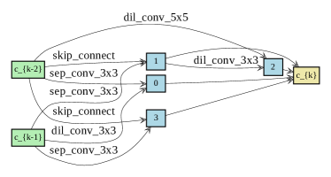
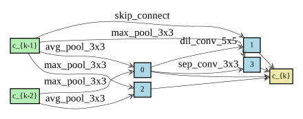
(a) Normal cells (left) and Reduce cells (right) for STL$\rightarrow$CIFAR10

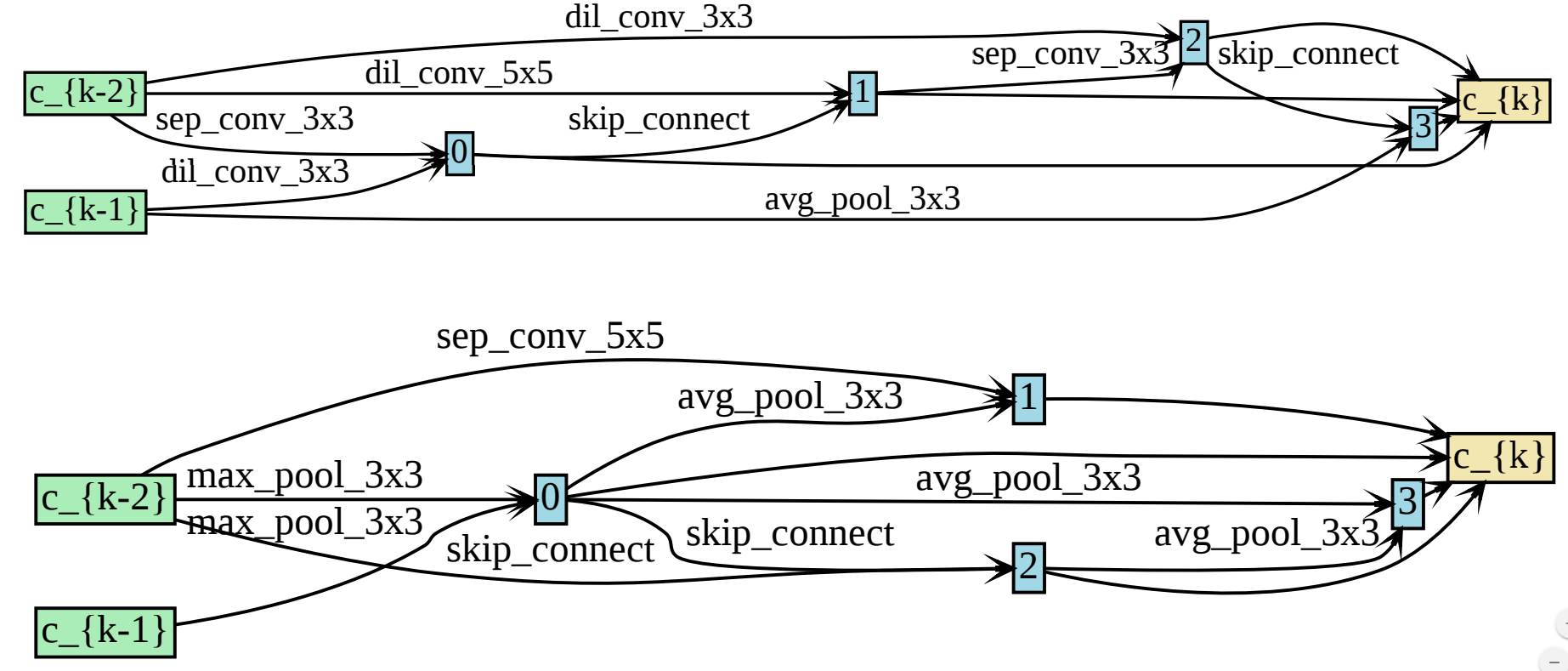
(b) Normal cells (upper) and Reduce cells (lower) for MNIST$\rightarrow$USPS

Method	Params (M)	Search Cost (GPU days)
NASNet zoph2018learning	3.3	1,800
AmoebaNet shah2018amoebanet	3.2	3,150
PNAS liu2018progressive	3.2	225
DARTS darts	3.3	1.5
SNAS xie2018snas	2.8	1.5
PDARTSchen2019progressive	3.4	0.3
NASDA	2.7	0.3

(c) Network architecture statistics comparison

Figure 2: (a) Neural architecture for STL$\rightarrow$CIFAR10 task. (b) Neural architecture for MNIST$\rightarrow$USPS results. (c) Comparison between our NASDA model and state-of-the-art NAS models.

We compare the proposed NASDA model with many state-of-the-art UDA baselines on multiple benchmarks. In the main paper, we only report major results; more details are provided in the supplementary material. All of our experiments are implemented in the PyTorch platform.

In the architecture search phase, we use $\lambda$=1 for all the searching experiments. We leverage the ReLU-Conv-BN order for convolutional operations, and each separable convolution is always applied twice (zoph2018learning, ; real2019regularized, ; liu2018progressive, ). Our search space $\mathcal{O}$ includes the following operations: $3\times 3$ and $5\times 5$ separable convolutions, $3\times 3$ and $5\times 5$ dilated separable convolutions, $3\times 3$ max pooling, identity, and $zero$. Our convolutional cell consists of $N=7$ nodes. Cells located at the $\frac{1}{3}$ and $\frac{2}{3}$ of the total depth of the network are reduction cells. The architecture encoding therefore is $(\alpha_{normal},\alpha_{reduce})$, where $\alpha_{normal}$ is shared by all the normal cells and $\alpha_{reduce}$ is shared by all the reduction cells. In the adversarial training phase, we set $N$=4 for all the experiments.

4.1 Setup

Digits We investigate three digits datasets: MNIST, USPS, and Street View House Numbers (SVHN). We adopt the evaluation protocol of CyCADA hoffman2017cycada with three transfer tasks: USPS to MNIST (U $\rightarrow$ M), MNIST to USPS (M $\rightarrow$ U), and SVHN to MNIST (S $\rightarrow$ M). We train our model using the training sets: MNIST (60,000), USPS (7,291), standard SVHN train (73,257).

STL$\rightarrow$CIFAR10 Both CIFAR10 cifar10 and STL stl10 are both 10-class image datasets. These two datasets contain nine overlapping classes. We remove the ‘frog’ class in CIFAR10 and the ‘monkey’ class in STL datasets as they have no equivalent in the other dataset, resulting in a 9-class problem. The STL images were down-scaled to 32$\times$32 resolution to match that of CIFAR10.

SYN SIGNS$\rightarrow$GTSRB We evaluated the adaptation from synthetic traffic signs dataset (SYN SIGNS dataset synthetic_sign ) to real-world signs dataset (GTSRB dataset GTSRB ). These datasets contain 43 classes.

We compare our NASDA model with state-of-the-art domain adaptation methods: Deep Adaptation Network (DAN) long2015 , Domain Adversarial Neural Network (DANN) DANN , Domain Separation Network (DSN) bousmalis2016domain , Coupled Generative Adversarial Networks (CoGAN) cogan , Maximum Classifier Discrepancy (MCD) MCD_2018 , Generate to Adapt (G2A) g2a , Stochastic Neighborhood Embedding (d-SNE) xu2019d , Associative Domain Adaptation (ASSOC) ASSC .

4.2 Empirical Results

Neural Architecture Search Results We show the neural architecture search results in Figure 2. We also show that our NASDA model contains less parameters and takes less time to converge compared with state-of-the-art NAS architectures. One interesting finding is that our NASDA contains more sequential connections in both Normal and Reduce cells when trained on MNIST$\rightarrow$USPS.

Table 1: Accuracy (%) on Digits and Traffic Signs for unsupervised domain adaptation.

Method	M $\rightarrow$ U	U $\rightarrow$ M	S $\rightarrow$ M	Avg(digits)	Method	SYN SIGNS $\rightarrow$ GTSRB
DAN li2017mmd	81.1	-	71.1	76.1	DAN li2017mmd	91.1
DANN DANN	85.1	73.0	71.1	76.4	DANN DANN	88.7
DSN dsn	$91.3$	-	82.7	-	DSN dsn	93.1
CoGAN cogan	$91.2^{*}$	89.1	-	-	CORAL sun2016deep	86.9
MCD MCD_2018	94.2	94.1	96.2	94.8	MCD MCD_2018	94.4
G2A g2a	95.0	90.8	92.4	92.7	ASSOC ASSC	82.8
SBADA-GAN sbada	95.3	97.6	76.1	89.7	SRDA-RAN srda	93.6
d-SNE xu2019d	99.0	98.7	96.5	98.1	DADRL DADRL	94.6
NASDA	98.0	98.7	98.6	98.4	NASDA	96.7

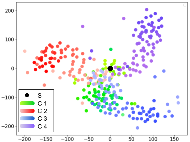
(a) T-SNE embedding for 4 classifiers’ weights

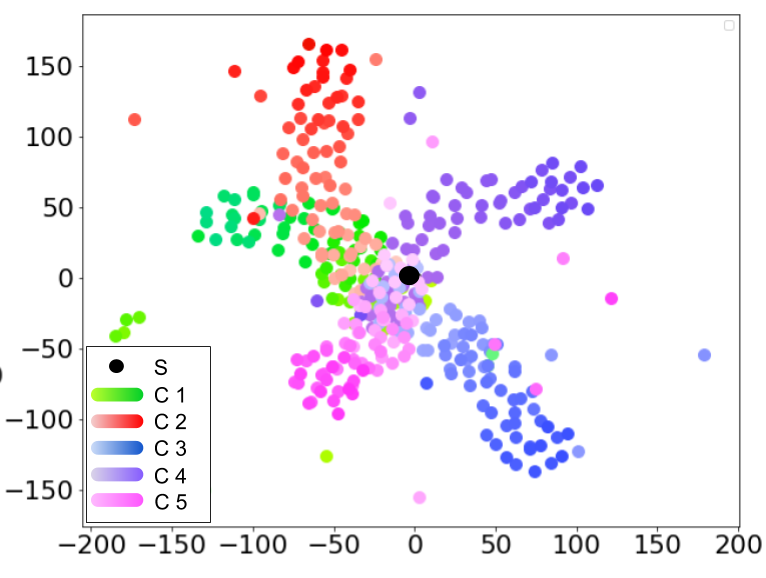
(b) T-SNE embedding for 5 classifiers’ weights

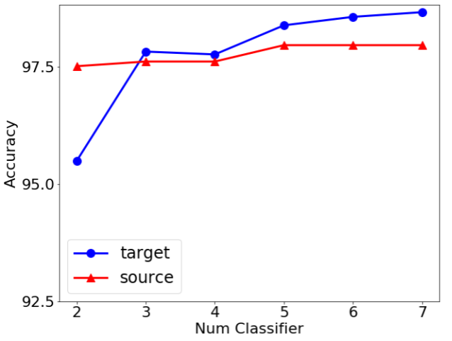
(c) Accuracy v.s. Classifier Number

Figure 3: (a)(b) We show the classifiers are diverged from each other in USPS$\rightarrow$MNIST task. (c) The relation between the source and target accuracy v.s. the number of classifiers in USPS$\rightarrow$MNIST task.

Unsupervised Domain Adaptation Results The UDA results for Digits and SYN SIGNS$\rightarrow$GTSRB are reported in Table 1, with results of baselines directly reported from the original papers if the protocol is the same (numbers with ^∗ indicates training on partial data). The NASDA model achieves a 98.4% average accuracy for Digits dataset, outperforming other baselines. For SYN SIGNS$\rightarrow$GTSRB task, our model gets comparable results with state-of-the-art baselines. The results demonstrate the effectiveness of our NASDA model on small images.

The UDA results on the STL$\rightarrow$CIFAR10 recognition task are reported in Table 2. Our model achieves a performance of 76.8%, outperforming all the baselines. To compare our search neural architecture with previous NAS models, we replace the neural architecture we used in $G$ with other NAS models.

Table 2: Accuracy (%) on STL $\rightarrow$ CIFAR10.

Method	STL $\rightarrow$ CIFAR10
DANN DANN	56.9
MCD MCD_2018	69.2
DWT roy2019unsupervised	71.2
SE french2017self	74.2
G2A g2a	72.8
VADA shu2018dirt	73.5
DIRT-T shu2018dirt	75.3
NASNet+Phase II zoph2018learning	67.3
AmoebaNet+Phase II shah2018amoebanet	67.0
DARTS+Phase II darts	68.8
PDARTS+Phase II chen2019progressive	66.0
NASDA	76.8

Other training settings in the second phase are identical to our model. As such, we derive NASNet+Phase II zoph2018learning , AmoebaNet+Phase II shah2018amoebanet , DARTS+Phase II darts , and PDARTS+Phase II chen2019progressive models. The results in Table 2 demonstrate that our model outperform other NAS based model by a large margin, demonstrating the effectiveness of our model in unsupervised domain adaptation.

Analysis To dive deeper into the training process of our NASDA model, we plot in Figure 3(a)-3(b) the T-SNE embedding of the weights of $C$ in USPS$\rightarrow$MNIST. This is achieved by recording the weights of all the classifiers for each epoch. The black dot indicates epoch zero, which is the common starting point. The color from light to dart corresponds to the epoch number from small to large. The T-SNE plots clearly show that the classifiers are diverged from each other, demonstrating the effectiveness of the second step of our NASDA training described in Section 3.2.

To explore the effect of the number of classifiers ($N$) on the final results, we plot the source and target accuracy v.s. the number of classifiers for USPS$\rightarrow$MNIST in Figure 3(c). The plot shows that with more classifiers, the accuracy of target domain increases significantly, while the accuracy of the source domain improves by a small margin. This is an interesting finding since it shows that the diversified classifiers boost the performance on the target domain. However, since the computation complexity of the adversarial loss defined by Equation (13) is $O(N^{2})$, the computation cost will increase quadratically when we increase $N$. We select $N$=4 for all our experiments, a trade-off between the performance and the computation efficiency.

5 Conclusion

In this paper, we first formulate a novel dual-objective task of Neural Architecture Search for Domain Adaptation (NASDA) to invigorate the design of transfer-aware network architectures. Towards tackling the NASDA task, we have proposed a novel learning framework that leverages MK-MMD to guide the neural architecture search process. Instead of aligning the features from existing handcrafted backbones, our model directly searches for the optimal neural architecture specific for domain adaptation. Furthermore, we have introduced the ways to consolidate the feature generator, which is stacked from the searched architecture, in order to boost the UDA performance. Extensive empirical evaluations on UDA benchmarks have demonstrated the efficacy of the proposed model against several state-of-the-art domain adaptation algorithms.

6 Broader Impacts

Data side The efficacy of deep learning algorithms highly relies on abundant labeled training data. However, annotating the large-scale dataset is tedious. In addition, labeling costs can be prohibitively expensive for some applications, requiring specialized expertise (labeling X-rays for medical diagnosis) or significant manual effort (pixel-level annotations for semantic segmentation). As such, reusing the learned knowledge from cheaper source of labels (e.g. existing labeled datasets, synthetic data) to generalize to new tasks and datasets is an critical but unsolved challenge.

Model side On the other hand, discovering state-of-the-art neural network architectures requires substantial effort of human experts. Recently, there has been a growing interest in developing algorithmic solutions to automate the manual process of architecture design. However, these models assume that the training and testing domain are sampled from the same distribution, neglecting the scenario where two data domains or multiple distributions are of interest.

Our work focuses on cost-efficient generalization by identifying a small subset of target data that will, once labeled, lead to good target performance. Specifically, we anticipate our line of work to automatically searching for the good deep backbone for knowledge transfer task. In terms of impact on society, this could mean that computer vision systems are able to better handle novel deployments and are less susceptible to dataset bias. For example, our system could adapt a traffic sign recognition system which is trained on simulated data to the real traffic sign recognition task. Although we do not experiment on fairness applications, domain adaptation has also been shown to improve the fairness of face recognition systems across race/gender.

Other negative impacts of our research on society are harder to predict, but it suffers from the same issues as most deep learning algorithms. These include adversarial attacks, privacy concerns and lack of interpretability, as well as other negative effects of increased automation. For example, it is not easy to interpret why the searched architecture is better to perform specific domain adaptation tasks.

7 Supplementary Material

7.1 Notations

We conclude all the notations we used in the paper in Table 3. Specifically, the notations with superscription “s” and “t” indicate they are from source domain and target domain, respectively.

Notation	Description
$\alpha$	Neural architecture parameters
$w$	Neural network weights
$\Phi$	Machine learning model
$P/Q$	Source / Target distribution
$G$	Feature generator in phase II
$C$	Classifier in phase II
$\mathcal{L}_{train}$ / $\mathcal{L}_{val}$	Training / Validation loss
$\mathbf{x}$ ($\mathbf{x}^{s}$, $\mathbf{x}^{t}$)	Training data (source, target)
$\mathbf{y}$ ($\mathbf{y}^{s}$, $\mathbf{y}^{t}$)	Labels (source, target)
$\mathcal{D}_{s}$ / $\mathcal{D}_{t}$	Source / Target Domain
$o^{(i,j)}$ / $e^{(i,j)}$	Operation / Edge from node i to j in NAS Graph
$x^{(i)}$	$i$-th node in a neural cell
$L$	Number of nodes in a neural cell
$d_{k}^{2}$ / $\hat{d}_{k}^{2}$	MK-MMD / Empirical MK-MMD
$k$ / $\mathcal{K}$	Kernel / Kernels
$m$	Number of data used to compute MK-MMD
$\xi$	Learning rate of inner optimization
$\lambda$	Trade-off parameters
$K$	Class number
$p(y|x)$	Probabilistic outputs of classifiers
$N$	Number of Classifiers

Table 3: We conclude all the notations we used in the paper.

7.2 Data Statistics

The datasets used in this paper are described in Table 4. Specifically, the USPS, MNIST, SVHN, CIFARO-10, STL datasets are from torchvision. The SYN SIGNS and GTSRB  dataset are downloaded from their official websites.

	# train	# test	# classes	Target	Resolution	Channels
USPS	7,291	2,007	10	Digits	$16\times 16$	Mono
MNIST	60,000	10,000	10	Digits	$28\times 28$	Mono
SVHN	73,257	26,032	10	Digits	$32\times 32$	RGB
CIFAR-10	50,000	10,000	10	Object ID	$32\times 32$	RGB
STL	5,000	8,000	10	Object ID	$96\times 96$	RGB
SYN SIGNS	100,000	–	43	Traffic signs	$40\times 40$	RGB
GTSRB	32,209	12,630	43	Traffic signs	varies	RGB

Table 4: Statistics of datasets we used in our paper.

Data Preparation Some of the experiments that involved datasets described in Table 4 required additional data preparation in order to match the resolution and format of the input samples and match the classification target. These additional steps will now be described.

STL $\rightarrow$ CIFAR-10 CIFAR-10 and STL are both 10-class image datasets. The STL images were down-scaled to $32\times 32$ resolution to match that of CIFAR-10. The ‘frog’ class in CIFAR-10 and the ‘monkey’ class in STL were removed as they have no equivalent in the other dataset, resulting in a 9-class problem with 10% less samples in each dataset.

Syn-Signs $\rightarrow$ GTSRB GTSRB is composed of images that vary in size and come with annotations that provide region of interest (bounding box around the sign) and ground truth classification. We extracted the region of interest from each image and scaled them to a resolution of $40\times 40$ to match those of Syn-Signs.

SVHN $\rightarrow$ MNIST The MNIST images were padded to $32\times 32$ resolution and converted to RGB by replicating the greyscale channel into the three RGB channels to match the format of SVHN.

7.3 Additional Experiment Results

In the paper, we report the result of SYN SIGNS$\rightarrow$GTSRB as 93.7%. After some grid search for the training hyper-parameters, we found that our model can actually achieve an accuracy of 96.7%, outperforming state-of-the-art baselines. All the results in Table 5 can be reproduced by the code we attached in the supplementary material.

Table 5: Accuracy (%) on Digits and Traffic Signs for unsupervised domain adaptation.

Method	M $\rightarrow$ U	U $\rightarrow$ M	S $\rightarrow$ M	Avg(digits)	Method	SYN SIGNS $\rightarrow$ GTSRB
DAN [78]	81.1	-	71.1	76.1	DAN [78]	91.1
DANN [12]	85.1	73.0	71.1	76.4	DANN [12]	88.7
DSN [79]	$91.3$	-	82.7	-	DSN [79]	93.1
CoGAN [9]	$91.2^{*}$	89.1	-	-	CORAL [80]	86.9
MCD [13]	94.2	94.1	96.2	94.8	MCD [13]	94.4
G2A [75]	95.0	90.8	92.4	92.7	ASSOC [77]	82.8
SBADA-GAN [81]	95.3	97.6	76.1	89.7	SRDA-RAN [82]	93.6
d-SNE [76]	99.0	98.7	96.5	98.1	DADRL [83]	94.6
NASDA	98.0	98.7	98.6	98.4	NASDA	96.7

7.4 ML reproducibility

We have submitted the code for all the experiments in the supplementary material. We will briefly describe the details about the experiments.

Hyper-parameter We set $\lambda$ to be 1 for all the experiments. The range of learning rate we considered is between 2e-4 to 0.25. We adopt grid search to select the best hyper-parameters. All the hyper-parameters used to generate results can be viewed in the code.

Measure For all the quantitative results in the paper, we use accuracy as the measurement.

Average runtime For Phase I in our model, i.e. searching the neural architecture, our model takes 0.3 GPU day to find the optimal architecture. For Phase II, our model typically takes about two days to converge.

Computing infrastructure Our code is based on Pytorch 1.2.0 and Torchvision 0.4.2. All other descriptions can be found in the readme file in the code.

References

- [1] Joaquin Quionero-Candela, Masashi Sugiyama, Anton Schwaighofer, and Neil D. Lawrence. Dataset Shift in Machine Learning. The MIT Press, 2009.
- [2] Mingsheng Long, Han Zhu, Jianmin Wang, and Michael I. Jordan. Deep transfer learning with joint adaptation networks. In Proceedings of the 34th International Conference on Machine Learning, ICML 2017, Sydney, NSW, Australia, 6-11 August 2017, pages 2208–2217, 2017.
- [3] Eric Tzeng, Judy Hoffman, Ning Zhang, Kate Saenko, and Trevor Darrell. Deep domain confusion: Maximizing for domain invariance. arXiv preprint arXiv:1412.3474, 2014.
- [4] Muhammad Ghifary, W Bastiaan Kleijn, and Mengjie Zhang. Domain adaptive neural networks for object recognition. In Pacific Rim international conference on artificial intelligence, pages 898–904. Springer, 2014.
- [5] Xingchao Peng and Kate Saenko. Synthetic to real adaptation with generative correlation alignment networks. In 2018 IEEE Winter Conference on Applications of Computer Vision, WACV 2018, Lake Tahoe, NV, USA, March 12-15, 2018, pages 1982–1991, 2018.
- [6] Mingsheng Long, Yue Cao, Jianmin Wang, and Michael Jordan. Learning transferable features with deep adaptation networks. In Francis Bach and David Blei, editors, Proceedings of the 32nd International Conference on Machine Learning, volume 37 of Proceedings of Machine Learning Research, pages 97–105, Lille, France, 07–09 Jul 2015. PMLR.
- [7] Baochen Sun and Kate Saenko. Deep CORAL: correlation alignment for deep domain adaptation. CoRR, abs/1607.01719, 2016.
- [8] Minghao Xu, Jian Zhang, Bingbing Ni, Teng Li, Chengjie Wang, Qi Tian, and Wenjun Zhang. Adversarial domain adaptation with domain mixup. arXiv preprint arXiv:1912.01805, 2019.
- [9] Ming-Yu Liu and Oncel Tuzel. Coupled generative adversarial networks. In Advances in neural information processing systems, pages 469–477, 2016.
- [10] Eric Tzeng, Judy Hoffman, Kate Saenko, and Trevor Darrell. Adversarial discriminative domain adaptation. In Computer Vision and Pattern Recognition (CVPR), volume 1, page 4, 2017.
- [11] Alexander H. Liu, Yen-Cheng Liu, Yu-Ying Yeh, and Yu-Chiang Frank Wang. A unified feature disentangler for multi-domain image translation and manipulation. CoRR, abs/1809.01361, 2018.
- [12] Yaroslav Ganin and Victor Lempitsky. Unsupervised domain adaptation by backpropagation. In Francis Bach and David Blei, editors, Proceedings of the 32nd International Conference on Machine Learning, volume 37 of Proceedings of Machine Learning Research, pages 1180–1189, Lille, France, 07–09 Jul 2015. PMLR.
- [13] Kuniaki Saito, Kohei Watanabe, Yoshitaka Ushiku, and Tatsuya Harada. Maximum classifier discrepancy for unsupervised domain adaptation. In The IEEE Conference on Computer Vision and Pattern Recognition (CVPR), June 2018.
- [14] Mingsheng Long, Zhangjie Cao, Jianmin Wang, and Michael I Jordan. Conditional adversarial domain adaptation. In Advances in Neural Information Processing Systems, pages 1640–1650, 2018.
- [15] Zili Yi, Hao (Richard) Zhang, Ping Tan, and Minglun Gong. Dualgan: Unsupervised dual learning for image-to-image translation. In ICCV, pages 2868–2876, 2017.
- [16] Jun-Yan Zhu, Taesung Park, Phillip Isola, and Alexei A Efros. Unpaired image-to-image translation using cycle-consistent adversarial networks. In Computer Vision (ICCV), 2017 IEEE International Conference on, 2017.
- [17] Judy Hoffman, Eric Tzeng, Taesung Park, Jun-Yan Zhu, Phillip Isola, Kate Saenko, Alexei Efros, and Trevor Darrell. CyCADA: Cycle-consistent adversarial domain adaptation. In Jennifer Dy and Andreas Krause, editors, Proceedings of the 35th International Conference on Machine Learning, volume 80 of Proceedings of Machine Learning Research, pages 1989–1998, Stockholmsmässan, Stockholm Sweden, 10–15 Jul 2018. PMLR.
- [18] Taeksoo Kim, Moonsu Cha, Hyunsoo Kim, Jung Kwon Lee, and Jiwon Kim. Learning to discover cross-domain relations with generative adversarial networks. In Doina Precup and Yee Whye Teh, editors, Proceedings of the 34th International Conference on Machine Learning, volume 70 of Proceedings of Machine Learning Research, pages 1857–1865, International Convention Centre, Sydney, Australia, 06–11 Aug 2017. PMLR.
- [19] Barret Zoph and Quoc V Le. Neural architecture search with reinforcement learning. ICLR, 2017.
- [20] Esteban Real, Alok Aggarwal, Yanping Huang, and Quoc V. Le. Aging evolution for image classifier architecture search. In AAAI 2019, 2019.
- [21] G Anandalingam and Terry L Friesz. Hierarchical optimization: An introduction. Annals of Operations Research, 34(1):1–11, 1992.
- [22] Barret Zoph, Vijay Vasudevan, Jonathon Shlens, and Quoc V Le. Learning transferable architectures for scalable image recognition. In Proceedings of the IEEE conference on computer vision and pattern recognition, pages 8697–8710, 2018.
- [23] Hanxiao Liu, Karen Simonyan, Oriol Vinyals, Chrisantha Fernando, and Koray Kavukcuoglu. Hierarchical representations for efficient architecture search. ICLR, 2018.
- [24] Chenxi Liu, Barret Zoph, Maxim Neumann, Jonathon Shlens, Wei Hua, Li-Jia Li, Li Fei-Fei, Alan Yuille, Jonathan Huang, and Kevin Murphy. Progressive neural architecture search. In Proceedings of the European Conference on Computer Vision (ECCV), pages 19–34, 2018.
- [25] Esteban Real, Alok Aggarwal, Yanping Huang, and Quoc V Le. Regularized evolution for image classifier architecture search. In Proceedings of the aaai conference on artificial intelligence, volume 33, pages 4780–4789, 2019.
- [26] Hanxiao Liu, Karen Simonyan, and Yiming Yang. Darts: Differentiable architecture search. International Conference on Learning Representations, 2019.
- [27] Arthur Gretton, Karsten M Borgwardt, Malte Rasch, Bernhard Schölkopf, and Alex J Smola. A kernel method for the two-sample-problem. In Advances in neural information processing systems, pages 513–520, 2007.
- [28] Karen Simonyan and Andrew Zisserman. Very deep convolutional networks for large-scale image recognition. CoRR, abs/1409.1556, 2014.
- [29] Kaiming He, Xiangyu Zhang, Shaoqing Ren, and Jian Sun. Deep residual learning for image recognition. In Proceedings of the IEEE conference on computer vision and pattern recognition, pages 770–778, 2016.
- [30] Christian Szegedy, Wei Liu, Yangqing Jia, Pierre Sermanet, Scott Reed, Dragomir Anguelov, Dumitru Erhan, Vincent Vanhoucke, and Andrew Rabinovich. Going deeper with convolutions. In Proceedings of the IEEE conference on computer vision and pattern recognition, pages 1–9, 2015.
- [31] Liang-Chieh Chen, Maxwell Collins, Yukun Zhu, George Papandreou, Barret Zoph, Florian Schroff, Hartwig Adam, and Jon Shlens. Searching for efficient multi-scale architectures for dense image prediction. In Advances in neural information processing systems, pages 8699–8710, 2018.
- [32] Mingxing Tan, Bo Chen, Ruoming Pang, Vijay Vasudevan, Mark Sandler, Andrew Howard, and Quoc V Le. Mnasnet: Platform-aware neural architecture search for mobile. In Proceedings of the IEEE Conference on Computer Vision and Pattern Recognition, pages 2820–2828, 2019.
- [33] Mingxing Tan and Quoc Le. EfficientNet: Rethinking model scaling for convolutional neural networks. In Kamalika Chaudhuri and Ruslan Salakhutdinov, editors, Proceedings of the 36th International Conference on Machine Learning, volume 97 of Proceedings of Machine Learning Research, pages 6105–6114, Long Beach, California, USA, 09–15 Jun 2019. PMLR.
- [34] Arber Zela, Aaron Klein, Stefan Falkner, and Frank Hutter. Towards automated deep learning: Efficient joint neural architecture and hyperparameter search. ICML 2018 Workshop on AutoML (AutoML 2018), 2018.
- [35] Aaron Klein, Stefan Falkner, Simon Bartels, Philipp Hennig, and Frank Hutter. Fast Bayesian Optimization of Machine Learning Hyperparameters on Large Datasets. In Aarti Singh and Jerry Zhu, editors, Proceedings of the 20th International Conference on Artificial Intelligence and Statistics, volume 54 of Proceedings of Machine Learning Research, pages 528–536, Fort Lauderdale, FL, USA, 20–22 Apr 2017. PMLR.
- [36] Patryk Chrabaszcz, Ilya Loshchilov, and Frank Hutter. A downsampled variant of imagenet as an alternative to the cifar datasets. arXiv preprint arXiv:1707.08819, 2017.
- [37] Tobias Domhan, Jost Tobias Springenberg, and Frank Hutter. Speeding up automatic hyperparameter optimization of deep neural networks by extrapolation of learning curves. In Twenty-Fourth International Joint Conference on Artificial Intelligence, 2015.
- [38] Kevin Swersky, Jasper Snoek, and Ryan Prescott Adams. Freeze-thaw bayesian optimization. arXiv preprint arXiv:1406.3896, 2014.
- [39] Aaron Klein, Stefan Falkner, Jost Tobias Springenberg, and Frank Hutter. Learning curve prediction with bayesian neural networks. ICLR, 2017.
- [40] Aditya Rawal and Risto Miikkulainen. From nodes to networks: Evolving recurrent neural networks. arXiv preprint arXiv:1803.04439, 2018.
- [41] Bowen Baker, Otkrist Gupta, Ramesh Raskar, and Nikhil Naik. Accelerating neural architecture search using performance prediction. NIPS Workshop on Meta-Learning, 2017.
- [42] Tao Wei, Changhu Wang, Yong Rui, and Chang Wen Chen. Network morphism. In International Conference on Machine Learning, pages 564–572, 2016.
- [43] Thomas Elsken, Jan-Hendrik Metzen, and Frank Hutter. Simple and efficient architecture search for convolutional neural networks. NIPS Workshop on Meta-Learning, 2017.
- [44] Han Cai, Tianyao Chen, Weinan Zhang, Yong Yu, and Jun Wang. Efficient architecture search by network transformation. In Thirty-Second AAAI conference on artificial intelligence, 2018.
- [45] Haifeng Jin, Qingquan Song, and Xia Hu. Auto-keras: An efficient neural architecture search system. In Proceedings of the 25th ACM SIGKDD International Conference on Knowledge Discovery & Data Mining, pages 1946–1956, 2019.
- [46] Han Cai, Jiacheng Yang, Weinan Zhang, Song Han, and Yong Yu. Path-level network transformation for efficient architecture search. International Conference on Machine Learning, 2018.
- [47] Shreyas Saxena and Jakob Verbeek. Convolutional neural fabrics. In Advances in Neural Information Processing Systems, pages 4053–4061, 2016.
- [48] Andrew Brock, Theodore Lim, James M Ritchie, and Nick Weston. Smash: one-shot model architecture search through hypernetworks. NIPS Workshop on Meta-Learning, 2017.
- [49] Hieu Pham, Melody Y Guan, Barret Zoph, Quoc V Le, and Jeff Dean. Efficient neural architecture search via parameter sharing. International Conference on Machine Learning, 2018.
- [50] Hanxiao Liu, Karen Simonyan, and Yiming Yang. Darts: Differentiable architecture search. International Conference on Learning Representations, 2019.
- [51] Gabriel Bender. Understanding and simplifying one-shot architecture search. International Conference on Machine Learning, 2018.
- [52] Han Cai, Ligeng Zhu, and Song Han. Proxylessnas: Direct neural architecture search on target task and hardware. International Conference on Learning Representations, 2019.
- [53] Sirui Xie, Hehui Zheng, Chunxiao Liu, and Liang Lin. Snas: stochastic neural architecture search. International Conference on Learning Representations, 2019.
- [54] Hieu Pham, Melody Y Guan, Barret Zoph, Quoc V Le, and Jeff Dean. Efficient neural architecture search via parameter sharing. International Conference on Machine Learning, 2018.
- [55] Shai Ben-David, John Blitzer, Koby Crammer, Alex Kulesza, Fernando Pereira, and Jennifer Wortman Vaughan. A theory of learning from different domains. Machine learning, 79(1-2):151–175, 2010.
- [56] Yishay Mansour, Mehryar Mohri, Afshin Rostamizadeh, and A R. Domain adaptation with multiple sources. In D. Koller, D. Schuurmans, Y. Bengio, and L. Bottou, editors, Advances in Neural Information Processing Systems 21, pages 1041–1048. Curran Associates, Inc., 2009.
- [57] Koby Crammer, Michael Kearns, and Jennifer Wortman. Learning from multiple sources. Journal of Machine Learning Research, 9(Aug):1757–1774, 2008.
- [58] Ruijia Xu, Ziliang Chen, Wangmeng Zuo, Junjie Yan, and Liang Lin. Deep cocktail network: Multi-source unsupervised domain adaptation with category shift. In Proceedings of the IEEE Conference on Computer Vision and Pattern Recognition, pages 3964–3973, 2018.
- [59] Lixin Duan, Dong Xu, and Shih-Fu Chang. Exploiting web images for event recognition in consumer videos: A multiple source domain adaptation approach. In Computer Vision and Pattern Recognition (CVPR), 2012 IEEE Conference on, pages 1338–1345. IEEE, 2012.
- [60] Xingchao Peng, Qinxun Bai, Xide Xia, Zijun Huang, Kate Saenko, and Bo Wang. Moment matching for multi-source domain adaptation. In Proceedings of the IEEE International Conference on Computer Vision, pages 1406–1415, 2019.
- [61] Arthur Gretton, Karsten M Borgwardt, Malte J Rasch, Bernhard Schölkopf, and Alexander Smola. A kernel two-sample test. Journal of Machine Learning Research, 13(Mar):723–773, 2012.
- [62] Xin Chen, Lingxi Xie, Jun Wu, and Qi Tian. Progressive differentiable architecture search: Bridging the depth gap between search and evaluation. In Proceedings of the IEEE International Conference on Computer Vision, pages 1294–1303, 2019.
- [63] Luca Franceschi, Paolo Frasconi, Saverio Salzo, Riccardo Grazzi, and Massimilano Pontil. Bilevel programming for hyperparameter optimization and meta-learning. ICML, 2018.
- [64] Fabian Pedregosa. Hyperparameter optimization with approximate gradient. 2016.
- [65] Dougal Maclaurin, David Duvenaud, and Ryan Adams. Gradient-based hyperparameter optimization through reversible learning. In International Conference on Machine Learning, pages 2113–2122, 2015.
- [66] Chelsea Finn, Pieter Abbeel, and Sergey Levine. Model-agnostic meta-learning for fast adaptation of deep networks. In Doina Precup and Yee Whye Teh, editors, Proceedings of the 34th International Conference on Machine Learning, volume 70 of Proceedings of Machine Learning Research, pages 1126–1135, International Convention Centre, Sydney, Australia, 06–11 Aug 2017. PMLR.
- [67] Jelena Luketina, Mathias Berglund, Klaus Greff, and Tapani Raiko. Scalable gradient-based tuning of continuous regularization hyperparameters. In International conference on machine learning, pages 2952–2960, 2016.
- [68] Abhishek Kumar, Prasanna Sattigeri, Kahini Wadhawan, Leonid Karlinsky, Rogerio Feris, Bill Freeman, and Gregory Wornell. Co-regularized alignment for unsupervised domain adaptation. In S. Bengio, H. Wallach, H. Larochelle, K. Grauman, N. Cesa-Bianchi, and R. Garnett, editors, Advances in Neural Information Processing Systems 31, pages 9345–9356. Curran Associates, Inc., 2018.
- [69] Syed Asif Raza Shah, Wenji Wu, Qiming Lu, Liang Zhang, Sajith Sasidharan, Phil DeMar, Chin Guok, John Macauley, Eric Pouyoul, Jin Kim, et al. Amoebanet: An sdn-enabled network service for big data science. Journal of Network and Computer Applications, 119:70–82, 2018.
- [70] Alex Krizhevsky, Geoffrey Hinton, et al. Learning multiple layers of features from tiny images. 2009.
- [71] Adam Coates, Andrew Ng, and Honglak Lee. An analysis of single-layer networks in unsupervised feature learning. In Proceedings of the fourteenth international conference on artificial intelligence and statistics, pages 215–223, 2011.
- [72] Boris Moiseev, Artem Konev, Alexander Chigorin, and Anton Konushin. Evaluation of traffic sign recognition methods trained on synthetically generated data. In Jacques Blanc-Talon, Andrzej Kasinski, Wilfried Philips, Dan Popescu, and Paul Scheunders, editors, Advanced Concepts for Intelligent Vision Systems, pages 576–583, Cham, 2013. Springer International Publishing.
- [73] Johannes Stallkamp, Marc Schlipsing, Jan Salmen, and Christian Igel. The German Traffic Sign Recognition Benchmark: A multi-class classification competition. In IEEE International Joint Conference on Neural Networks, pages 1453–1460, 2011.
- [74] Konstantinos Bousmalis, George Trigeorgis, Nathan Silberman, Dilip Krishnan, and Dumitru Erhan. Domain separation networks. In Advances in neural information processing systems, pages 343–351, 2016.
- [75] Swami Sankaranarayanan, Yogesh Balaji, Carlos D Castillo, and Rama Chellappa. Generate to adapt: Aligning domains using generative adversarial networks. In Proceedings of the IEEE Conference on Computer Vision and Pattern Recognition, pages 8503–8512, 2018.
- [76] Xiang Xu, Xiong Zhou, Ragav Venkatesan, Gurumurthy Swaminathan, and Orchid Majumder. d-sne: Domain adaptation using stochastic neighborhood embedding. In Proceedings of the IEEE Conference on Computer Vision and Pattern Recognition, pages 2497–2506, 2019.
- [77] P. Haeusser, T. Frerix, A. Mordvintsev, and D. Cremers. Associative domain adaptation. In 2017 IEEE International Conference on Computer Vision (ICCV), pages 2784–2792, 2017.
- [78] Chun-Liang Li, Wei-Cheng Chang, Yu Cheng, Yiming Yang, and Barnabás Póczos. Mmd gan: Towards deeper understanding of moment matching network. In Advances in Neural Information Processing Systems, pages 2203–2213, 2017.
- [79] Konstantinos Bousmalis, George Trigeorgis, Nathan Silberman, Dilip Krishnan, and Dumitru Erhan. Domain separation networks. In Advances in Neural Information Processing Systems, pages 343–351, 2016.
- [80] Baochen Sun and Kate Saenko. Deep coral: Correlation alignment for deep domain adaptation. In European conference on computer vision, pages 443–450. Springer, 2016.
- [81] Paolo Russo, Fabio M Carlucci, Tatiana Tommasi, and Barbara Caputo. From source to target and back: symmetric bi-directional adaptive gan. In Proceedings of the IEEE Conference on Computer Vision and Pattern Recognition, pages 8099–8108, 2018.
- [82] Guanyu Cai, Yuqin Wang, and Lianghua He. Learning smooth representation for unsupervised domain adaptation, 2019.
- [83] V. Tran and C. Huang. Domain adaptation meets disentangled representation learning and style transfer. In 2019 IEEE International Conference on Systems, Man and Cybernetics (SMC), pages 2998–3005, 2019.
- [84] Subhankar Roy, Aliaksandr Siarohin, Enver Sangineto, Samuel Rota Bulo, Nicu Sebe, and Elisa Ricci. Unsupervised domain adaptation using feature-whitening and consensus loss. In Proceedings of the IEEE Conference on Computer Vision and Pattern Recognition, pages 9471–9480, 2019.
- [85] Geoffrey French, Michal Mackiewicz, and Mark Fisher. Self-ensembling for visual domain adaptation. arXiv preprint arXiv:1706.05208, 2017.
- [86] Rui Shu, Hung H Bui, Hirokazu Narui, and Stefano Ermon. A dirt-t approach to unsupervised domain adaptation. arXiv preprint arXiv:1802.08735, 2018.