Non-Markovian Majority-Vote model

Abstract

Non-Markovian dynamics pervades human activity and social networks and it induces memory effects and burstiness in a wide range of processes including inter-event time distributions, duration of interactions in temporal networks and human mobility. Here we propose a non-Markovian Majority-Vote model (NMMV) that introduces non-Markovian effects in the standard (Markovian) Majority-Vote model (SMV). The SMV model is one of the simplest two-state stochastic models for studying opinion dynamics, and displays a continuous order-disorder phase transition at a critical noise. In the NMMV model we assume that the probability that an agent changes state is not only dependent on the majority state of his neighbors but it also depends on his age, i.e. how long the agent has been in his current state. The NMMV model has two regimes: the aging regime implies that the probability that an agent changes state is decreasing with his age, while in the antiaging regime the probability that an agent changes state is increasing with his age. Interestingly, we find that the critical noise at which we observe the order-disorder phase transition is a non-monotonic function of the rate $\beta$ of the aging (antiaging) process. In particular the critical noise in the aging regime displays a maximum as a function of $\beta$ while in the antiaging regime displays a minimum. This implies that the aging/antiaging dynamics can retard/anticipate the transition and that there is an optimal rate $\beta$ for maximally perturbing the value of the critical noise. The analytical results obtained in the framework of the heterogeneous mean-field approach are validated by extensive numerical simulations on a large variety of network topologies.

I Introduction

Many natural, social and technological phenomena can be well described by stochastic binary-state models formed by a large number of interacting agents. Depending on the application, various types of dynamical rules determining the stochastic switch of the states of the agents can be considered. This framework includes very well known processes, such as the Ising model, the voter model and the susceptible-infected-susceptible model, that have been used to model magnetic materials Baxter (1989), opinion formation Castellano et al. (2009); Redner (2017), and epidemic spreading Pastor-Satorras et al. (2015); Wang et al. (2016), among others Muñoz (2018); Perc et al. (2017). Strikingly, extensions or modifications for the models can lead in a variety of cases to dynamical behaviors drastically different from the original ones. For example, the presence of non-trivial structure in the interacting patterns such as heavy-tailed degree distribution Pastor-Satorras et al. (2015); Dorogovtsev et al. (2008), mesoscopic structures Fortunato (2010); Chen et al. (2018), multilayer structures Boccaletti et al. (2014); Bianconi (2018); Halu et al. (2013), can induce significant change in the dynamics. Moreover, relevant effect can be obtained also changing the dynamical rules by introducing of more than two states Wu (1982); Starnini et al. (2012), time delay Kim and Noh (2017), nonhomogeneous interevent intervals Fernández-Gracia et al. (2011); Takaguchi and Masuda (2011); Min et al. (2011, 2013), a fraction of zealot Mobilia (2003); Khalil et al. (2018) or latency period Lambiotte et al. (2009).

The Majority-Vote (MV) model is a simple non-equilibrium Ising-like system with up-down symmetry that presents an order-disorder phase transition at a critical value of noise de Oliveira (1992). The MV model is also one of the paradigmatic models for studying opinion dynamics, and it has been extensively studied in regular lattices Kwak et al. (2007); Wu and Holme (2010); Acuña Lara et al. (2014); Acuña Lara and Sastre (2012); Yu (2017), random graphs Pereira and Moreira (2005); Lima et al. (2008), and in complex networks including small-world networks Campos et al. (2003); Luz and Lima (2007); Stone and McKay (2015), scale-free networks Lima (2006); Lima and Malarz (2006); Chen et al. (2015); Huang et al. (2017), modular networks Huang et al. (2015), complete graphs Fronczak and Fronczak (2017), and spatial networks Sampaio Filho et al. (2016). Some extensions were also proposed, such as multi-state MV models Brunstein and Tomé (1999); Tomé and Petri (2002); Chen and Li (2018); Melo et al. (2010); Li et al. (2016); Lima (2012); Costa and de Souza (2005), inertial effect Chen et al. (2017a, b); Harunari et al. (2017), frustration due to anticonformists Krawiecki (2018), and cooperation in multilayer structures Choi and Goh (2018); Liu et al. (2019).

Most of stochastic binary-state models are based on a memoryless Markovian assumption, which implies that the switching rates from one state to the other depend only on the present state of the system. One of important properties of Markovian processes is that the inter-event time intervals follow an exponential distribution and the number of events in a given time interval follows a Poissonian distribution. The Markovian assumption facilitates theoretical analysis of models. However, there is growing evidence that human activity follows a non-Markovian dynamics driven by memory effects. Non-Markovian bursty dynamics characterized by heavy tail inter-event time distributions is ubiquitous in human activities Karsai et al. (2018); Barabasi (2005); Vázquez et al. (2006); González et al. (2008); Vazquez et al. (2007); Iribarren and Moro (2009); Karsai et al. (2011),and strongly affects the duration of interactions in temporal networks Zhao et al. (2011a, b); Stehlé et al. (2010). Memory effects have also shown to be essential to model human mobility and random walks over complex networks González et al. (2008); Brockmann et al. (2006); Rosvall et al. (2014). Therefore, the Markovian assumption provides only an approximate picture of the real world.

In recent years, there is an increasing interest in understanding the role of non-Markovian effects in stochastic binary-state models, from the theoretical Van Mieghem and van de Bovenkamp (2013); Jo et al. (2014); Kiss et al. (2015a); Starnini et al. (2017); Kiss et al. (2015b); Feng et al. (2019) and from the numerical Boguñá et al. (2014); Masuda and Rocha (2018) perspective as well.

One important development of non-Markovian effects in stochastic binary-state models have been introduced by assuming that the switching probability between states depends on the age of the agent, i.e., how long an agent has been in its current state Stark et al. (2008); Pérez et al. (2016). The induced effects of this non-Markovian dynamics are also called aging effects when the switching probability decreases with the agent’s age and antiaging effects when the switching probability increases with the agent’s age. These non-Markovian effects usually induce a slow-down of the relaxation dynamics toward the stationary state. In particular in social systems they can be related to behavioral inertia accounting for a tendency for a belief or an opinion to endure once formed.

A very important class of models describing opinion dynamics is the voter model and its variations. In the standard voter model, each agent updates his state by copying the state of one of his neighbors. The model exhibits ordering dynamics toward either of consensus states in finite-size systems Redner (2017). The effects of introducing a non-Markovian dynamics within the voter model and its variations have been considered in several works. In Ref. Stark et al. (2008), Stark et al. reported a counter-intuitive phenomenon induced by aging in the voter model. They showed that the transition probability between two opposite states decreases with age, but the time to reach a macroscopically ordered state can be accelerated. In Ref. Peralta et al. (2020a), Peralta et al. studied systematically the aging version of the voter model at the mean-field level, and they showed that the model reaches consensus or gets trapped in a frozen state depending on the specific form describing the transition probability and the nodes’ age. They also considered the antiaging case when the transition probability is an increasing function of age. For the latter case, the model always reaches a steady state with coexistence of two states. In the noisy voter model, additional stochastic effects are introduced in the opinion dynamics. In particular given an agent of a noisy voter model and his randomly selected neighbor, the agent does not adopt the neighbor opinion deterministically. An important consequence of this is that a stationary state can be achieved without consensus Peralta et al. (2018). In Refs. Artime et al. (2018, 2019), it has been shown that the aging effects in the noisy voter model can alter the character of the phase transition. In the absence of aging, the model show a finite-size discontinuous transition between ordered and disordered phases. When the aging is introduced, the transition becomes a well defined second order transition observed in the thermodynamic limit. Moreover, recently Peralta et al. in Ref. Peralta et al. (2020b) proved that the non-Markovian noisy voter model can be approximately reduced to a non-linear noisy voter model which is Markovian.

In the present work, we reveal the role of non-Markovian dynamics in the Majority-Vote (MV) model providing results that enrich the scenario depicted by the works above summarized. In the MV model each agent tends to agree with the majority state of his neighbors, and disagreement only occurs with probability $f$. Here $f$ can be interpreted as the internal noise due to imperfect information exchange or uncertainty on the states of neighbors. As $f$ increases, the MV model shows a continuous order-disorder transition belonging to the universality class of the equilibrium Ising model de Oliveira (1992). In particular, for $f=0$ the MV model is equivalent to the zero-temperature Ising model with Glauber dynamics Zhou and Lipowsky (2005).

It is interesting to discuss the difference between the MV model and the voter model and its variations. The main difference of the MV model with respect to the voter model is that at each time in the MV model each agent changes opinion depending on the majority of its neighbors while in the voter model each agent changes opinion depending on the state of a single randomly selected neighbor. Moreover in the standard voter model the system reaches consensus while this is not the case in the MV model. The noisy voter model is closer to MV model as in both models we can reach a stationary state with a majority opinion but without consensus. However due to the different dynamical rules the nature of the phase transition observed in the two models is different as demonstrated by the different universality class of the ordering dynamics of the voter model Sood and Redner (2005); Castellano et al. (2005).

Here we propose the non-Markovian Majority-Vote (NMMV) model by incorporating non-Markovian dynamics in the Majority-Vote model. In the NMMV model, the transition probability between states not only depends on the majority state of the agent’s neighbors and noise inetensity $f$, but also depends on the agent’s age. Specifically, the NMMV model includes two regimes: the aging regime in which the probability of a state switch decreases with the agent’s age and an antiaging regime in which the probability of a state switch increases with the agent’s age. We indicate with $\beta$ the rate of change of the transition probability with age. The NMMV model also displays a continuous phase transition as a function of $f$: for $f<f_{c}^{NMMV}$ the NMMV model is in the ordered phase, i.e., the network displays a clear majority state, for $f\geq f_{c}^{NMMV}$ the NMMV is in the disordered phase where no global majority state exist. We show that the non-Markovian dynamics strongly affects the value of the critical noise $f_{c}^{NMMV}$. In particular, in the aging regime the non-Markovian dynamics retards the transition with respect to the standard Majority-Vote model (SMV) and the critical noise $f_{c}^{NMMV}$ in the NMMV model is larger or equal to the critical noise $f_{c}^{SMV}$ in the SMV model, i.e., $f_{c}^{NMMV}\geq f_{c}^{SMV}$. In the antiaging regime, instead, the relation between the critical noise in the NMMV model and in the SMV model are reversed, i.e., $f_{c}^{NMMV}\leq f_{c}^{SMV}$. Interestingly, by solving the model in the framework of an heterogeneous mean-field approach, we can derive analytically the non-monotonic dependence of the critical noise $f_{c}^{NMMV}$ on the rate $\beta$. In the aging regime, the critical noise displays a maximum at a non-zero but finite value of $\beta$. In the antiaging regime, a minimum of the critical noise as a function of $\beta$ is found. This means that the non-Markovian dynamics can be used to retard or anticipate the transition.

The theoretical mean-field predictions are in good agreement with extensive simulations of the model.

The paper is structured as follows: in Sec. II we define the NMMV model; in Sec. III we present the analytic solution of the model obtained in the framework of the heterogeneous mean-field approach; in Sec. IV we characterize the critical properties of the model including the analytical expression of the critical noise, and its dependence on the rate $\beta$; in Sec. V we compare the analytic predictions to the simulation results; finally in Sec. VI we provide the conclusions.

II Majority-Vote Model with non-Markovian switching of states

In this section we introduce the non-Markovian Majority-Vote model which differs from the standard Majority-Vote model de Oliveira (1992) by introducing a non-Markovian mechanism for the switching of states. Therefore in the NMMV model the agents have a probability of switching states that depends on their age, i.e. for how long they have been in their current state.

We consider a population of $N$ agents defined on a static network topology. Each agent $i$ with $i=1,\cdots,N$ is located on a node $i$ of the network. Each agent is assigned two dynamical variables: a binary variable $\sigma_{i}=\pm 1$ (his state) describing the agent’s opinion/vote and a variable $a_{i}$ (his age) indicating for how long the agent has not changed his state. Initially the states $\{\sigma_{i}\}$ are randomly assigned to the agents and the variables $\{a_{i}\}$ are initialized by setting $a_{i}=0$ for every agent $i$ of the network. At each time step, an agent $i$ is chosen at random and his state is switched with probability $w_{i}$ which implements the non-Markovian Majority Vote process. Thus with probability $w_{i}$, the agent $i$ switches state and the age of agent $i$ is reset to zero, i.e.,

$$\sigma_{i} \rightarrow -\sigma_{i},$$

$$a_{i} \rightarrow 0.$$ (1)

Otherwise, nothing happens except for the age increased by one, i.e.,

$$a_{i}\rightarrow a_{i}+1.$$ (2)

In both cases the time is updated according to

$$t\to t+\Delta t,$$ (3)

with $\Delta t=1/N$. The richness of the model resides on the definition of the switching probability $w_{i}$ given by

$$w_{i}=\nu_{i}w_{i}^{SMV},$$ (4)

where $0\leq\nu_{i}\leq 1$, called the activation probability, is a function of the age $a_{i}$ of agent $i$ and where $w_{i}^{SMV}$ is the switching probability in the SMV model, i.e., it is independent of the age variable. The contribution $w_{i}^{SMV}$ to the switching probability $w_{i}$ of the agent $i$ depends on the majority state of $i^{\prime}$s neighborhood and on a parameter $f$ called the noise intensity. If the state $\sigma_{i}$ of the agent is opposite to the majority state of his neighbors, $w_{i}^{SMV}$ contributes to the switching probability to the majority state by a term $1-f$. If the state $\sigma_{i}$ of the agent is the same as the majority state of his neighbors, $w_{i}^{SMV}$ contributes to the switching probability to the majority state by a term $f$. If there is no clear majority of the agent $i$’s neighbors, i.e., half of the neighbors have state $\sigma_{j}=+1$ and half of the neighbors have state $\sigma_{j}=-1$, then $w_{i}^{SMV}=1/2.$ Therefore, $w_{i}^{SMV}$ can be expressed as

$${w_{i}^{SMV}}{\rm{=}}\frac{{\rm{1}}}{{\rm{2}}}\left[{{\rm{1-}}\left({{\rm{1-2}}f}\right){\sigma_{i}}S\left({\sum\limits_{j\in{\mathcal{N}_{i}}}{{\sigma_{j}}}}\right)}\right],$$ (5)

where $\mathcal{N}_{i}$ denotes the set of neighbors of agent $i$, and $S(x)$, defined as $S(x)=\mbox{sgn}(x)$ if $x\neq 0$ and $S(0)=0$, indicates the majority state of his neighborhood.

The NMMV model reduces to the SMV model in the case in which we consider a trivial choice of $\nu_{i}$, i.e. $\nu_{i}=1$ for all agent $i$. In this case, as $f$ increases, the model undergoes a continuous order-disorder phase transition at a critical value of noise intensity $f=f_{c}^{SMV}$ Chen et al. (2015).

However, in a number of real scenarios for social and human dynamics it has been shown that non-Markovian effects are relevant Karsai et al. (2018). Indeed a large number of human activity including written correspondence, emails (Barabasi, 2005), mobile phone communication Zhao et al. (2011a) is not memoryless, on the contrary it is characterized by important non-Markovian effects typically leading to intermittent and bursty dynamics.

Different models for explaining the emergence of bursty dynamics have been proposed (see for a review Ref.Karsai et al. (2018)). Interestingly, a model Stehlé et al. (2010); Zhao et al. (2011b, a) explaining the occurrence of bursty human dynamics of social interactions assumes that a number of feedback mechanisms affect human behavior, which introduce memory effects in the rate at which an agent to change his state. In particular in this framework it is assumed that each agent does not change his state at a constant rate in time, rather the rate at which he changes his state depends on the time elapsed since he adopted his current state. This framework, originally proposed to model the duration of social interactions is a very general framework that can be also applied to opinion dynamics. In opinion dynamics this framework will give rise to a simple yet very general phenomenological model to describe the inertia of the agents in retaining their own opinion. By following these considerations, here we capture the effect of the non-Markovian opinion dynamics in the MV model by assuming that the probability $\nu_{i}$ at which an agent $i$ changes opinion depends on how long the agent has retained its current opinion, i.e.

$$\nu_{i}=\nu(a_{i}),$$ (6)

where $a_{i}$ indicates the age of agent $i$. In the following we will consider several different functional forms for the function $\nu(a)$ including exponential, linear, rational, and power-law dependence with the the age $a$. To start with a concrete example let us now consider the exponential form for $\nu(a)$, given by

$$\nu(a)=\left({{\nu_{0}}-{\nu_{\infty}}}\right){e^{-\beta a}}+{\nu_{\infty}},$$ (7)

where $\nu_{0}=\nu(0)$ and $\nu_{\infty}=\lim_{a\to\infty}\nu(a)$.

The probability $\nu(a)$ capture the non-Markovian nature of the dynamics and is parametrized by the parameter $\beta>0$. Note that $\beta$ characterizes the rate of exponential change of $\nu$ as a function of $a$. Obviously, in the limits of $\beta\rightarrow 0$ and $\beta\rightarrow\infty$, all the agents have the same fixed value of activity, $\nu\equiv\nu_{0}$ and $\nu\equiv\nu_{\infty}$, and the dynamics is thus equivalent to the SMV model with the time scaled by a factor $\nu_{0}^{-1}$ and $\nu_{\infty}^{-1}$, respectively.

We distinguish two different regimes of the dynamics:

• Aging regime. For $\nu_{0}>\nu_{\infty}$, $\nu(a)$ decays exponentially with $a$, implying that the longer an agent is in a given state, the more difficult is for him to change state.

• Antiaging regime. For $\nu_{0}<\nu_{\infty}$, $\nu(a)$ increases exponentially with $a$. Such an case can be interpreted as “rejuvenating” dynamics where agents become more prone to change state as they are longer on a given state.

Without loss of generality, set equal to one the maximum between $\nu_{0}$ and $\nu_{\infty}$, i.e. we put $\max\left\{{{\nu_{0}},{\nu_{\infty}}}\right\}=1$. Moreover, to avoid trivial frozen states of the dynamics, the minimum between $\nu_{0}$ and $\nu_{\infty}$ is set to be larger than zero, i.e., $\min\left\{{{\nu_{0}},{\nu_{\infty}}}\right\}>0$.

III Heterogeneous mean-field solution of the model

In order to capture the phase diagram of the NMMV model on a random network with given degree distribution $P(k)$, we solve the model using the heterogeneous mean-field approach  Dorogovtsev et al. (2008). Therefore we assume that the probability that an agent $i$ is in a given state depends exclusively on his degree $k$ and his age $a$ and we denote by $x_{k,a}^{\pm}$ the probability that an agent of degree $k$ has age $a$ and is in the state $\pm 1$. It follows that the probability $x_{k}^{\pm}$ of an agent of degree $k$ in the state $\pm 1$, is given by

$$x_{k}^{\pm}=\sum\nolimits_{a=0}^{\infty}{x_{k,a}^{\pm}}.$$ (8)

In order to solve the dynamical equations of the NMMV model in the heterogeneous mean-field approximation we also need to evaluate the switching probability $w_{k,a}^{\pm}$ of an agent of degree $k$ and age $a$. Let us define ${{\tilde{x}}^{\pm}}$ the probability that by following a link we reach a node in state $\pm 1$, given by

$${{\tilde{x}}^{\pm}}=\sum\limits_{k}{\frac{{kP\left(k\right)}}{{\left\langle k\right\rangle}}x_{k}^{\pm}}=\sum\limits_{k}{\frac{{kP\left(k\right)}}{{\left\langle k\right\rangle}}\sum\limits_{a=0}^{\infty}{x_{k,a}^{\pm}}}.$$ (9)

For a node of degree $k$, the probability that the majority state among his neighborhoods is $\pm 1$ is given by the binomial distribution,

$${\psi_{k}}\left({{{\tilde{x}}^{\pm}}}\right)=\sum\limits_{n=\left\lceil{k/2}\right\rceil}^{k}{\left({1-\frac{1}{2}{\delta_{n,k/2}}}\right)C_{k}^{n}}{\left({{{\tilde{x}}^{\pm}}}\right)^{n}}{\left({1-{{\tilde{x}}^{\pm}}}\right)^{k-n}},$$

(10)

where $\left\lceil\cdot\right\rceil$ is the ceiling function, $\delta_{r,s}$ is the Kronecker symbol, and $C_{k}^{n}={{k!}\mathord{\left/{\vphantom{{k!}{\left[{n!\left({k-n}\right)!}\right]}}}\right.\kern-1.2pt}{\left[{n!\left({k-n}\right)!}\right]}}$ are the binomial coefficients. According to Eq.(4), we can write down the switching probability $w_{k,a}^{\pm}$ of an agent of state $\pm 1$ with degree $k$ and age $a$ as

$$w_{k,a}^{\pm}=\nu\left({a+1}\right){\Psi_{k}}\left({{{\tilde{x}}^{\pm}}}\right),$$ (11)

where $\nu(a+1)$ is given by Eq.(7), and ${\Psi_{k}}\left({{{\tilde{x}}^{\pm}}}\right)$ is the flipping probability of an agent of state $\pm 1$ without the aging effect  Chen et al. (2015), i.e.,

$${\Psi_{k}}\left({{{\tilde{x}}^{\pm}}}\right)=\left({1-f}\right)\left[{1-{\psi_{k}}\left({{{\tilde{x}}^{\pm}}}\right)}\right]+f{\psi_{k}}\left({{{\tilde{x}}^{\pm}}}\right).$$ (12)

The dynamical equations that determine the time evolution of the probabilities $x_{k,a}^{\pm}$ are a function of the switching probabilities $w_{k,a}^{\pm}$. These equations can be deduced by observing that at each time step one of the following four possible events occurs.

• An agent in state $+1$ having degree $k$ and age $a$ is chosen and his state is flipped. The rate at which $x_{k,a}^{+}$ decreases and $x_{k,0}^{-}$ increases due to this process is $x_{k,a}^{+}w_{k,a}^{+}$.

• An agent in state $+1$ having degree $k$ and age $a$ is chosen but his state is not flipped. The rate at which $x_{k,a}^{+}$ decreases and $x_{k,a+1}^{+}$ increases due to this process is $x_{k,a}^{+}(1-w_{k,a}^{+})$.

• An agent in state $-1$ having degree $k$ and age $a$ is chosen and the state is flipped. The rate at which $x_{k,a}^{-}$ decreases and $x_{k,0}^{+}$ increases due to this process is $x_{k,a}^{-}w_{k,a}^{-}$.

• An agent in state $-1$ having degree $k$ and age $a$ is chosen but the state is not flipped. The rate at which $x_{k,a}^{-}$ decreases and $x_{k,a+1}^{-}$ increases due to this process is $x_{k,a}^{-}(1-w_{k,a}^{-})$.

Accordingly, the rate equations for $x_{k,a}^{\pm}$ read

$$\frac{{dx_{k,0}^{+}}}{{dt}} = \sum\limits_{a=0}^{\infty}{x_{k,a}^{-}w_{k,a}^{-}}-x_{k,0}^{+},$$ (13)

$$\frac{{dx_{k,a}^{+}}}{{dt}} = x_{k,a-1}^{+}\left({1-w_{k,a-1}^{+}}\right)-x_{k,a}^{+},{\kern 10.0pt}a\geq 1,$$ (14)

$$\frac{{dx_{k,0}^{-}}}{{dt}} = \sum\limits_{a=0}^{\infty}{x_{k,a}^{+}w_{k,a}^{+}}-x_{k,0}^{-},$$ (15)

$$\frac{{dx_{k,a}^{-}}}{{dt}} = x_{k,a-1}^{-}\left({1-w_{k,a-1}^{-}}\right)-x_{k,a}^{-},{\kern 10.0pt}a\geq 1.$$ (16)

In stationary state, by setting the time derivative of $x_{k,a}^{\pm}$ equal to zero, we obtain that the probabilities $x_{k,a}^{\pm}$ obey

$$x_{k,0}^{+} = \sum\limits_{a=0}^{\infty}{x_{k,a}^{-}w_{k,a}^{-}},$$ (17)

$$x_{k,a}^{+} = x_{k,a-1}^{+}\left({1-w_{k,a-1}^{+}}\right),{\kern 10.0pt}a\geq 1,$$ (18)

$$x_{k,0}^{-} = \sum\limits_{a=0}^{\infty}{x_{k,a}^{+}w_{k,a}^{+}},$$ (19)

$$x_{k,a}^{-} = x_{k,a-1}^{-}\left({1-w_{k,a-1}^{-}}\right),{\kern 10.0pt}a\geq 1.$$ (20)

Using Eq.(18) and Eq.(19), and summing $x_{k,a}^{+}$ over the values of $a$ greater or equal to one we get

$$x_{k,0}^{+}=x_{k,0}^{-}.$$ (21)

This condition is a necessary condition for stationarity. In fact, at stationarity the probability that a node is in a given state does not change with time, or equivalently the expected number of agents in state $+1$ that change their state (and reset their age to $a=0$) should be equal to the number of agent in state $-1$ that change their state (and reset their age to $a=0$) Artime et al. (2018).

In terms of Eq.(18) and Eq.(20), $x_{k,a}^{\pm}$ for $a\geq 1$ can be computed in a recursive way, and then are expressed by $x_{k,0}^{\pm}$,

$$\begin{array}[]{lr}x_{k,a}^{\pm}=x_{k,0}^{\pm}{F_{k,a}}\left({{{\tilde{x}}^{\pm}}}\right),&a\geq 1,\end{array}$$ (23)

where for convenience we have introduced the function $F_{k,a}$, given by

$${F_{k,a}}\left({{{\tilde{x}}^{\pm}}}\right)=\prod\limits_{j=0}^{a-1}{\left[{1-w_{k,j}^{\pm}\left({{{\tilde{x}}^{\pm}}}\right)}\right]}.$$ (24)

Substituting Eq.(23) into the definition $x_{k}^{\pm}=\sum\nolimits_{a=0}^{\infty}{x_{k,a}^{\pm}}$, we have

$$x_{k}^{\pm}=x_{k,0}^{\pm}F_{k}\left({{{\tilde{x}}^{\pm}}}\right),$$ (25)

with

$$F_{k}\left({{{\tilde{x}}^{\pm}}}\right){\rm{=1+}}\sum\limits_{a=0}^{\infty}{{F_{k,a}}\left({{{\tilde{x}}^{\pm}}}\right)}.$$ (26)

In order to find $x_{k}^{+}$ we note that by using Eq.(21), we can express the ratio $x_{k}^{+}/x_{k}^{-}$ as

$$\frac{{x_{k}^{+}}}{{x_{k}^{-}}}=\frac{{x_{k,0}^{+}}}{{x_{k,0}^{-}}}\frac{{F_{k}\left({{{\tilde{x}}^{\rm{+}}}}\right)}}{{F_{k}\left({{{\tilde{x}}^{-}}}\right)}}=\frac{{F_{k}\left({{{\tilde{x}}^{\rm{+}}}}\right)}}{{F_{k}\left({{{\tilde{x}}^{-}}}\right)}}.$$ (27)

Substituting ${\tilde{x}}^{-}$ with $1-{\tilde{x}}^{+}$ in Eq.(27), we then obtain

$$x_{k}^{+}=\frac{{F_{k}\left({{{\tilde{x}}^{\rm{+}}}}\right)}}{{F_{k}\left({{{\tilde{x}}^{\rm{+}}}}\right)+F_{k}\left({1-{{\tilde{x}}^{+}}}\right)}}.$$ (28)

Finally by using Eq.(28) in the left-hand side of Eq.(9), we find the self-consistent equation of $\tilde{x}^{+}$,

$${{\tilde{x}}^{+}}=\sum\limits_{k}{\frac{{kP\left(k\right)}}{{\left\langle k\right\rangle}}\frac{{F_{k}\left({{{\tilde{x}}^{\rm{+}}}}\right)}}{{F_{k}\left({{{\tilde{x}}^{\rm{+}}}}\right)+F_{k}\left({1-{{\tilde{x}}^{+}}}\right)}}}.$$ (29)

This equation can be solved numerically by finding $\tilde{x}^{+}$ by iterating Eq.(29) starting from an initial value of $\tilde{x}^{+}\neq 1/2$. Once $\tilde{x}^{+}$ is found, we can calculate $x_{k}^{+}$ by using Eq.(28). This allow us to find the average magnetization per node by

$$m=\sum\nolimits_{k}{P\left(k\right)\left({x_{k}^{+}-x_{k}^{-}}\right)}=\sum\nolimits_{k}{P\left(k\right)\left({2x_{k}^{+}-1}\right)}.$$ (30)

This theoretical treatment of the model provides predictions that can be compared to simulation results revealing the critical properties of the NMMV model. In particular, the main features of the steady state configurations can be described by plotting $m$ as a function of $f$ for different values of $\beta$.

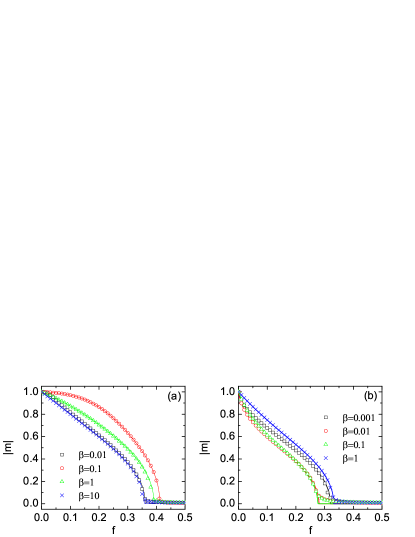
Figure 1: The absolute value of $m$, $|m|$, is plotted as a function of the noise $f$ for several values of $\beta$. Panel (a) shows $|m|$ versus $f$ for $\nu_{0}>\nu_{\infty}$, i.e. for a dynamics in the aging regime; panel (b) shows $|m|$ versus $f$ for $\nu_{0}<\nu_{\infty}$, i.e. for a dynamics in the antiaging regime. The simulations (symbols) performed on a regular random network (RR) with $N=10^{4}$ nodes and with degree of the nodes given by $\left\langle k\right\rangle=20$ are compared with theoretical predictions (solid lines). All results are obtained for $\max\left\{{{\nu_{0}},{\nu_{\infty}}}\right\}=1$ and $\min\left\{{{\nu_{0}},{\nu_{\infty}}}\right\}=0.05$.

In Fig.1(a), we report such results for $\nu_{0}>\nu_{\infty}$, when the non-Markovian dynamics is in the aging regime. Here we have used regular random networks (RR) whose degree distribution follows a delta function, $P(k)=\delta\left({k-\left\langle k\right\rangle}\right)$ with $\left\langle k\right\rangle=20$ and network size $N=10^{4}$. Direct simulation results are compared to theoretical predictions finding excellent agreement (see Fig.1). The order parameter $|m|$ shows a continuous second-order phase transition as noise intensity $f$ varies, similar to the SMV model. The transition point, i.e., the critical value of noise intensity $f_{c}^{NMMV}$, depends on the value of $\beta$. In the aging regime, as $\beta$ increases, $f_{c}^{NMMV}$ displays a maximum at $\beta=\beta_{m}^{aging}$. In the antiaging regime ($\nu_{0}<\nu_{\infty}$), $f_{c}^{NMMV}$ shows again a non-monotonous behavior but instead of displaying a maximum as a function of $\beta$ (like in presence of the aging dynamics) it displays a minimum at $\beta=\beta_{m}^{antiaging}$ (see Fig.1(b)).

IV The phase diagram

IV.1 The critical noise

In this paragraph we will use the heterogeneous mean-field approach to derive the expression for the critical noise $f_{c}^{NMMV}$ in the NMMV model. First of all, we notice that $\tilde{x}^{+}=1/2$, is always a solution of Eq.(29). This state corresponds to the disordered phase where the state of each agent is totally random. Such a trivial solution loses its stability when the noise intensity is less than a critical value, i.e., $f<f_{c}^{NMMV}$. According to linear stability analysis, the critical noise $f_{c}^{NMMV}$ can be found by imposing that the derivative of the right-hand side of Eq.(29) with respect to $\tilde{x}^{+}$ calculated for $\tilde{x}^{+}=1/2$ is equal to one, i.e., $f_{c}^{NMMV}$ satisfies

$$\sum\limits_{k}{\frac{{kP\left(k\right)}}{{\left\langle k\right\rangle}}\frac{{F^{\prime}_{k}\left({\frac{1}{2}}\right)}}{{2F_{k}\left({\frac{1}{2}}\right)}}}=1.$$ (31)

At $\tilde{x}^{+}=1/2$, $\psi_{k}$ and also $\Psi_{k}$ are independent of $k$. In particular we have ${\Psi_{k}}\left({\frac{1}{2}}\right)=\frac{1}{2}$ for all value of $k$. Therefore using Eq.(26), this implies that also $F_{k}\left({\frac{1}{2}}\right)$ is independent of $k$ and is given by

$${F}\left({\frac{1}{2}}\right)=1+\sum\limits_{a=1}^{\infty}{{F_{a}}}\left({\frac{1}{2}}\right),$$ (32)

with

$${F_{a}}\left({\frac{1}{2}}\right)=\prod\limits_{j=1}^{a}{\left({1-\frac{1}{2}\nu\left(j\right)}\right)},$$ (33)

(note that here we have omitted the subscript $k$ in the expression of $F_{k}(\frac{1}{2})$ and $F_{k,a}(\frac{1}{2})$ as they do not depend on $k$.) After some simple algebra, we can express $F^{\prime}_{k}\left({\frac{1}{2}}\right)$ as

$$F^{\prime}_{k}\left({\frac{1}{2}}\right)=-\Psi_{k}^{\prime}\left({\frac{1}{2}}\right)\sum\limits_{a=1}^{\infty}{{F_{a}}\left({\frac{1}{2}}\right)\sum\limits_{j=1}^{a}{\frac{{{\nu(j)}}}{{1-\frac{1}{2}{\nu(j)}}}}},$$ (34)

with

$$\Psi^{\prime}_{k}\left({\frac{1}{2}}\right)=\left({2f-1}\right)\psi^{\prime}_{k}\left({\frac{1}{2}}\right),$$ (35)

and

$$\psi^{\prime}_{k}\left({\frac{1}{2}}\right)={2^{1-k}}kC_{k-1}^{\left\lceil{\left({k-1}\right)/2}\right\rceil}.$$ (36)

Substituting Eqs.(32-36) into Eq.(31), we obtain the critical noise $f_{c}^{NMMV}$ in the NMMV model,

$$f_{c}^{NMMV}=\frac{1}{2}-G\left({\beta;{\nu_{0}},{\nu_{\infty}}}\right)\frac{{\left\langle k\right\rangle}}{{\sum\nolimits_{k}{{k^{2}}P\left(k\right){2^{1-k}}C_{k-1}^{\left\lceil{\left({k-1}\right)/2}\right\rceil}}}},$$

(37)

where

$$G\left({\beta;{\nu_{0}},{\nu_{\infty}}}\right)=\frac{{F\left({\frac{1}{2}}\right)}}{{\sum\limits_{a=1}^{\infty}{{F_{a}}\left({\frac{1}{2}}\right)\sum\limits_{j=1}^{\infty}{\frac{{{\nu(j)}}}{{1-\frac{1}{2}{\nu(j)}}}}}}}.$$ (38)

Using Stirling’s approximation for large $k$, $C_{k-1}^{\left\lceil{\left({k-1}\right)/2}\right\rceil}\approx{{{2^{k-1}}}\mathord{\left/{\vphantom{{{2^{k-1}}}{\sqrt{{{k\pi}\mathord{\left/{\vphantom{{k\pi}2}}\right.\kern-1.2pt}2}}}}}\right.\kern-1.2pt}{\sqrt{{{k\pi}\mathord{\left/{\vphantom{{k\pi}2}}\right.\kern-1.2pt}2}}}}$, Eq.(37) can be simplified to

$$f_{c}^{NMMV}=\frac{1}{2}-G\left({\beta;{\nu_{0}},{\nu_{\infty}}}\right)\sqrt{\frac{\pi}{2}}\frac{{\left\langle k\right\rangle}}{{\left\langle{{k^{3/2}}}\right\rangle}},$$ (39)

where $\langle\ldots\rangle$ denotes the average over the degree distribution $P(k)$. The critical noise $f_{c}^{NMMV}$ dependence on the non-Markovian dynamics is fully captured by the function $G\left({\beta;{\nu_{0}},{\nu_{\infty}}}\right)$, which can be considered as a function of $\beta$ for any given value of the parameters $\nu_{0}$ and $\nu_{\infty}$. We distinguish two main regimes:

• For $\nu_{0}>\nu_{\infty}$, $G\left({\beta;{\nu_{0}},{\nu_{\infty}}}\right)$ captures the dependence of $f_{c}^{NMMV}$ on $\beta$ in the aging regime;

• For $\nu_{0}<\nu_{\infty}$, $G\left({\beta;{\nu_{0}},{\nu_{\infty}}}\right)$ captures the dependence of $f_{c}^{NMMV}$ on $\beta$ in the antiaging regime.

When the aging effects are not taken into account, $\nu(a)\equiv\nu$, $G\left({\beta;{\nu_{0}},{\nu_{\infty}}}\right)=\frac{1}{2}$, and Eq.(39) thus reduces to the expression of the critical noise in the SMV model Chen et al. (2015),

$$f_{c}^{SMV}=\frac{1}{2}-\frac{1}{2}\sqrt{\frac{\pi}{2}}\frac{{\left\langle k\right\rangle}}{{\left\langle{{k^{3/2}}}\right\rangle}}.$$ (40)

IV.2 The function $G\left({\beta;{\nu_{0}},{\nu_{\infty}}}\right)$

As noted before, the function $G\left({\beta;{\nu_{0}},{\nu_{\infty}}}\right)$ captures all the dependence of the critical noise $f_{c}^{NMMV}$ on the non-Markovian dynamics. In particular, from Eq.(39) and Eq.(40) we deduce that the function $G\left({\beta;{\nu_{0}},{\nu_{\infty}}}\right)$ characterizes the relation between the critical noise in NMMV model and in the SMV model. In fact, we have

$$2G\left({\beta;{\nu_{0}},{\nu_{\infty}}}\right)=\frac{1/2-f_{c}^{NMMV}}{1/2-f_{c}^{SMV}},$$ (41)

The numerical solution of Eq.(38) reveals that the function $G\left({\beta;{\nu_{0}},{\nu_{\infty}}}\right)$ displays a non-monotonous behavior as a function of $\beta$ when $\nu_{0}$ and $\nu_{\infty}$ are fixed to a constant value. In particular, the function $G\left({\beta;{\nu_{0}},{\nu_{\infty}}}\right)$ displays a minimum as a function of $\beta$ in the aging regime and a maximum in the antiaging regime (see Fig.2). In the limit $\beta\rightarrow 0$ or $\beta\rightarrow\infty$, we obtain $G\left({\beta;{\nu_{0}},{\nu_{\infty}}}\right)\rightarrow 1/2$ indicating the marginal role of the non-Markovian dynamics, i.e., using Eq.(41) $f_{c}^{NMMV}\to f_{c}^{SMV}$. Since the critical noise $f_{c}^{NMMV}$ depends on $\beta$ only through the function $G\left({\beta;{\nu_{0}},{\nu_{\infty}}}\right)$ in the aging regime, the minimum of $G\left({\beta;{\nu_{0}},{\nu_{\infty}}}\right)$ is achieved for $\beta=\beta_{m}^{aging}$, corresponding to the maximum of $f_{c}^{NMMV}$; conversely in the antiaging regime the maximum of $G\left({\beta;{\nu_{0}},{\nu_{\infty}}}\right)$ is achieved for $\beta=\beta_{m}^{antiaging}$ corresponding to the minimum of $f_{c}^{NMMV}$. Let us indicate with $\Delta G_{m}$ the maximal deviation of the function $G$ from its asymptotic value $1/2$ achieved in the limit $\beta\rightarrow 0$ and $\beta\rightarrow\infty$, i.e.,

$$\Delta G_{m}=\left|\frac{1}{2}-G\left({\beta_{m}};{\nu_{0}},{\nu_{\infty}}\right)\right|.$$ (42)

Specifically let us indicate with $\Delta G_{m}^{aging}$ the values obtained in the aging regime and with $\Delta G_{m}^{antiaging}$ the values obtained in the antiaging regime.

Therefore, the values of $\Delta G_{m}^{aging}$ and $\Delta G_{m}^{antiaging}$ characterize the maximal difference between $f_{c}^{NMMV}$ and $f_{c}^{SMV}$ for the aging regime and antiaging regime, respectively. We note that since $G$ is independent of the topology of the underlying network, $\beta_{m}^{aging}$ ($\beta_{m}^{antiaging}$) at which $f_{c}^{NMMV}$ is maximized (minimized), is not affected by the network topology.

While the definition of $G$ given by Eq.(38) is valid for arbitrary functions $\nu(a)$, the investigation performed in this paragraph is obtained starting from the expression for $\nu(a)$ given by Eq.(7). However, here we conjecture that these results do not qualitatively change for other choices of the function $\nu(a)$ as long as the derivative of function is monotonic. This is strictly speaking the case in which we can properly use the terms aging and antiaging for dynamical evolution as an inflection point in $\nu(a)$ (corresponding to a maximum or minimum in the derivative $d\nu/da$) will introduce a characteristic scale $a=a^{\star}$ on the dynamics.

In order to check this conjecture we have considered several functions $\nu(a)$ with a monotonic first derivative.

In particular, we have considered the linear function

$$\nu\left(a\right)=\left\{\begin{array}[]{l}\beta\left({\nu_{\infty}-\nu_{0}}\right)a+\nu_{0},{\kern 10.0pt}a<1/\beta,\\ \nu_{\infty},{\kern 10.0pt}a\geq 1/\beta,\end{array}\right.$$ (45)

the rational function

$$\nu\left(a\right)=\frac{{\nu_{\infty}a+\nu_{0}/\beta}}{{a+1/\beta}},$$ (46)

and the expression

$$\nu\left(a\right)=\left({\nu_{0}-\nu_{\infty}}\right){\left({1+a}\right)^{-\beta}}+\nu_{\infty}.$$ (47)

including a power-law dependence on the age $a$. Interestingly, the functional dependences given by Eq.(46) and Eq.(47) reproduce non-Markovian dynamics observed in inter-event times and duration of social contact (see for a review Ref. Karsai et al. (2018)). We have studied the function $G\left({\beta;{\nu_{0}},{\nu_{\infty}}}\right)$ for all these kernels, and we have found that qualitatively the results are unchanged with respect to the results obtained for the exponential kernel.

In Fig. 3 we show the dependence of $\beta_{m}^{aging}$, $\beta_{m}^{antiaging}$ and of $\Delta G_{m}^{aging}$ and $\Delta G_{m}^{antiaging}$ as a function of $\min\left\{{{\nu_{0}},{\nu_{\infty}}}\right\}$ for the four types of kernel with a fixed value of $\max\left\{{{\nu_{0}},{\nu_{\infty}}}\right\}=1$. We observe that while $\Delta G_{m}^{aging}$, $\Delta G_{m}^{antiaging}$ and $\beta_{m}^{antiaging}$ show the same monotonic trend for all the kernels, $\beta_{m}^{aging}$ displays a different trend depending on the considered kernels. Indeed while for the linear and exponential kernels both $\beta_{m}^{aging}$, increase with $\min\left\{{{\nu_{0}},{\nu_{\infty}}}\right\}$, for the rational and power-law kernels it decreases with $\min\left\{{{\nu_{0}},{\nu_{\infty}}}\right\}$.

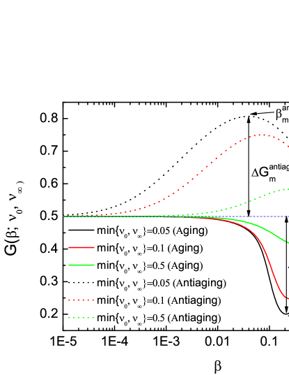
Figure 2: The function $G\left({\beta;{\nu_{0}},{\nu_{\infty}}}\right)$ defined in Eq.(38) is plotted as a function of $\beta$ in the aging regime (for $\nu_{0}>\nu_{\infty}$) and in the antiaging regime (for $\nu_{0}<\nu_{\infty}$). All curves are obtained for $\max\left\{{{\nu_{0}},{\nu_{\infty}}}\right\}=1$.

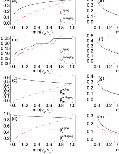
Figure 3: In the left panels, the values of $\beta_{m}^{aging}$ and $\beta_{m}^{antiaging}$ are plotted versus $\min\left\{{{\nu_{0}},{\nu_{\infty}}}\right\}$. In the right panels, the values of $\Delta G_{m}^{aging}$ and $\Delta G_{m}^{antiaging}$ are plotted as a function of $\min\left\{{{\nu_{0}},{\nu_{\infty}}}\right\}$. From the top to bottom, we consider four functional forms for $\nu(a)$ are considered: exponential (Eq.7), linear (Eq.45), rational (Eq.46), and power-law (Eq.47) kernels. All curves are obtained for $\max\left\{{{\nu_{0}},{\nu_{\infty}}}\right\}=1$.

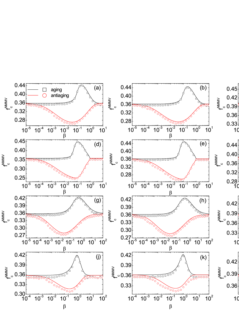
Figure 4: The critical noise $f_{c}^{NMMV}$ is plotted as a function of $\beta$ in the aging and antiaging regimes for three different networks (from left to right: the regular-random networks (RR) with degree of each node $\left\langle k\right\rangle=20$, the Erdös-Rényi (ER) random networks with average degree $\left\langle k\right\rangle=20$, and scale-free networks with degree distribution exponent $\gamma=3$ and minimal degree $k_{min}=10$) and four types of $\nu(a)$ (from top to bottom: exponential (Eq.7), linear (Eq.45), rational (Eq.46), and power-law (Eq.47) kernels). Symbols and lines show the simulation and theoretical results, respectively. All curves are obtained by setting $\max\left\{{{\nu_{0}},{\nu_{\infty}}}\right\}=1$ and $\min\left\{{{\nu_{0}},{\nu_{\infty}}}\right\}=0.05$. We have also performed simulations with some other values of $\min\left\{{{\nu_{0}},{\nu_{\infty}}}\right\}$, and found that the non-monotonic behavior of $f_{c}^{NMMV}$ is qualitatively the same.

V Comparison with numerical results

In this section we compare the results obtained analytically using the heterogeneous mean-field approximation with extensive numerical results on different network topologies.

We have considered three different random networks generated using the configuration model Newman et al. (2001):

• regular random networks (RR) with degree distribution $P\left(k\right)=\delta\left({k-\left\langle k\right\rangle}\right)$;

• Erdös-Rényi networks (ER) with degree distribution $P\left(k\right)={{{e^{-\left\langle k\right\rangle}}{{\left\langle k\right\rangle}^{k}}}\mathord{\left/{\vphantom{{{e^{-\left\langle k\right\rangle}}{{\left\langle k\right\rangle}^{k}}}{k!}}}\right.\kern-1.2pt}{k!}}$;

• scale-free networks (SF) with degree distribution $P\left(k\right)\sim k^{-\gamma}$.

In order to numerically determine the critical noise $f_{c}^{NMMV}$, we calculated the Binder’s fourth-order cumulant $U$ Binder (1997), defined as

$$U=1-\frac{1}{3}\frac{\left[{\overline{m^{4}}}\right]}{\left[{\overline{m^{2}}}\right]^{2}},$$ (48)

where $m=\sum_{i}^{N}\sigma_{i}/N$ is the average magnetization per node, $\overline{\cdot}$ denotes the time averages taken in the stationary regime, and $\left[\cdot\right]$ indicates the averages over different network configurations. The critical noise $f_{c}^{NMMV}$ is obtained by detecting the point $f=f_{c}^{NMMV}$ where the curves $U=U(f)$ obtained for different network sizes $N$, intercept each other. In Fig.4, we show $f_{c}^{NMMV}$ as a function of $\beta$ for the aging and antiaging regime for the three considered network models and for the four types of considered kernels without characteristic scale, finding very good agreement with the mean-field theoretical predictions despite these latter neglect the correlations present in the NMMV.

As predicted by the mean-field theory, for all the considered choices of $\nu(a)$ without inflection point, the critical noise $f_{c}^{NMMV}$ shows a non-monotonic dependence on $\beta$ in both regimes. In the aging regime, there exists an optimal value of $\beta$ in which $f_{c}^{NMMV}$ is maximized, in the antiaging regime instead $f_{c}^{NMMV}$ displays a minimum as a function of $\beta$. The optimal $\beta$ for the two regimes are independent of the network degree distribution as predicted by the heterogeneous mean-field solution.

However, this scenario can change if the function $\nu(a)$ describes a dynamics with a characteristic scale. This is not typically the scenario considered in physical works investigating the slow down of the dynamics due to aging, but it is actually a very valuable choice in the present context of social opinion dynamics. To investigate this case here we focus on the class of logistic functions $\nu(a)$ given by

$$\nu(a)=\frac{\nu_{0}-\nu_{\infty}}{1+e^{\beta(a-a^{\star})}}+\nu_{\infty},$$ (49)

with both $a^{\star}$ and $\beta$ being non-negative. This logistic function is a monotonic function of $a$ and for large values of $\beta$ approaches a step function at $a=a^{\star}$. Most notably this choice of functional for, for $\nu(a)$ introduces a characteristic scale $a=a^{\star}$ for age at which the change of opinion occurs.

We have simulated the NMMV model with this logistic kernel and compared the theory with the analytical mean-field prediction finding satisfactory agreement between the two (see Fig. 5).

Interestingly in this case we observe that only for $a^{\star}=0$ (where there is no effective typical scale in the system) we recover the same qualitative behavior of $f^{NMMV}$ observed in the previous kernels (see Fig. 4). We therefore make the important observation that the introduction of a typical scale $a=a^{\star}$ can significantly alter the phenomenology of the process.

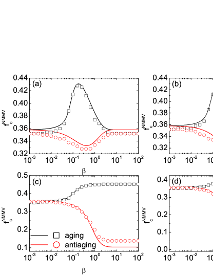
Figure 5: The critical noise $f_{c}^{NMMV}$ is plotted as a function of $\beta$ in the aging and antiaging regime for four different values of $a^{\star}$ when $\nu(a)$ takes the logistic form given by Eq.(49). From (a)-(d), $a^{\star}=0$, 1, 5, and 10, respectively. We have used the regular random networks with degree of each node given by $k=20$. Symbols and lines show the simulation and theoretical results, respectively. All results are obtained by setting $\max\left\{{{\nu_{0}},{\nu_{\infty}}}\right\}=1$ and $\min\left\{{{\nu_{0}},{\nu_{\infty}}}\right\}=0.05$.

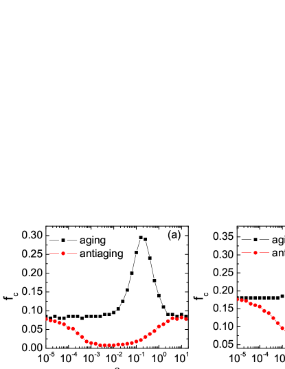
Figure 6: The critical noise $f_{c}^{NMMV}$ is plotted as a function of $\beta$ in the aging and antiaging regime for a 2d square lattices (panel a) and in 3d cubic lattices (panel b) where we have take the exponential kernel $\nu(a)$ given by Eq. (7). All results are obtained setting $\max\left\{{{\nu_{0}},{\nu_{\infty}}}\right\}=1$ and $\min\left\{{{\nu_{0}},{\nu_{\infty}}}\right\}=0.05$.

Finally, we investigated the NMMV model also on two-dimensional and three-dimensional regular lattices, which are network topologies for which the heterogeneous mean-field approximation is not valid. For these lattices we have exclusively considered the exponential kernel given by Eq. (7). The results are shown in Fig.6. For two-dimensional lattices, the critical noise shows a maximum $f^{NMMV}_{c}\approx 0.3$ at $\beta_{m}^{aging}\approx 0.2$ in the aging regime and a minimum $f^{NMMV}_{c}\approx 0.008$ at $\beta_{m}^{antiaging}\approx 0.01$ in the antiaging regime. For three-dimensional lattices, the critical noise shows a maximum $f^{NMMV}_{c}\approx 0.36$ at $\beta_{m}^{aging}\approx 0.2$ in the regime regime and a minimum $f^{NMMV}_{c}\approx 0.05$ at $\beta_{m}^{antiaging}\approx 0.01$ in the antiaging regime. In the limits of $\beta\rightarrow 0$ and $\beta\rightarrow\infty$, the critical noise tend respectively to $0.075$ and $0.18$ in two-dimensional and three-dimensional lattices, consistent with the results valid for the SMV model Yang et al. (2008). This result shows evidently that also in situations in which we are far from the conditions necessary for the application of the heterogeneous approximation we observe a non-monotonic dependence of the critical noise $f_{c}^{NMMV}$ of the NMMV model on $\beta$ revealing that the observed phenomenology is universal, i.e., it is independent of the network topology.

VI Conclusion

In this work we have introduced the non-Markovian Majority-Vote (NMMV) model that differs from the standard Majority-Vote (SMV) model as it includes memory effects. In fact in the NMMV model the probability that an agent switches state (activation probability) is not only dependent on the majority state of its neighbours as for the SMV model, but it is also age-dependent, i.e. depends on how long a agent has been in the same state (his age $a$) captured by the function $\nu(a)$.

We distinguish two regime of the NMMV model: the aging regime in which the activation probability is a decreasing function of the agent’s age, and the antiaging regime in which the activation probability is an increasing function of the agent’s age. We call $\beta$ the rate determining the change of the activation probability with the age of the agent. The NMMV model displays a phase transition as a function of the noise $f$ determining the probability that an agent switches to the minority state of its neighbors. For $f<f_{c}^{NMMV}$ the NMMV model is in an ordered phase and displays an overall majority state, for $f\geq f_{c}^{NMMV}$ the model is in a disordered phase in which half of the agents are in one state and the other half of the agents are in the other state.

By analytically solving the model using the heterogeneous mean-field approach and by performing extensive numerical simulations, we reveal how the non-Markovian dynamics affects the critical noise $f_{c}^{NMMV}.$

These results indicate that in the aging regime the non-Markovian dynamics retards the transition, and in the antiaging dynamics it anticipates the transition. Interestingly the most significant effect of the non-Markovian dynamics is achieved at a finite and non-zero value of the rate $\beta$, indicating that the aging/antiaging dynamics needs to have a characteristic time-scale that is neither too fast or too slow.

Interestingly, as long as the non-Markovian kernel $\nu(a)$ does not have a characteristic scale, the critical noise $f_{c}^{NMMV}$ in the NMMV model exhibits a non-monotonic dependence on the rate $\beta$ at which the activation probability changes with age. In particular we found two opposite behaviors in the aging and in the antiaging regimes. In the aging regime, the critical noise $f_{c}^{NMMV}$ displays a maximum as a function of $\beta$ in the antiaging regime instead $f_{c}^{NMMV}$ displays a minimum as a function of $\beta$.

Finally, this work highlights the importance of non-Markovian dynamics in determining the phase diagram of the NMMV model and we hope that it will stimulate interest in further investigations of the effect of memory and non-Markovian dynamics in critical phenomena defined on networks.