Multi-wavelength modelling of the circumstellar environment of the massive proto-star AFGL 2591 VLA 3

Abstract

We have studied the dust density, temperature and velocity distributions of the archetypal massive young stellar object (MYSO) AFGL 2591. Given its high luminosity ($L=2\times 10^{5}\,\mbox{L${}_{\sun}$}$) and distance ($d=3.3$ kpc), AFGL 2591 has one of the highest $\sqrt{L}/d$ ratio, giving better resolved dust emission than any other MYSO. As such, this paper provides a template on how to use resolved multi-wavelength data and radiative transfer to obtain a well-constrained 2-D axi-symmetric analytic rotating infall model. We show for the first time that the resolved dust continuum emission from Herschel 70 µm observations is extended along the outflow direction, whose origin is explained in part from warm dust in the outflow cavity walls. However, the model can only explain the kinematic features from CH₃CN observations with unrealistically low stellar masses ($<15$ M_☉), indicating that additional physical processes may be playing a role in slowing down the envelope rotation. As part of our 3-step continuum and line fitting, we have identified model parameters that can be further constrained by specific observations. High-resolution mm visibilities were fitted to obtain the disc mass (6 M_☉) and radius (2200 au). A combination of SED and near-IR observations were used to estimate the luminosity and envelope mass together with the outflow cavity inclination and opening angles.

1 Introduction

High-mass stars play an important role in the evolution of galaxies, but their formation is still not well understood. Do high-mass stars form as a scaled-up version of isolated low-mass star formation (e.g. Krumholz et al., 2012; Kuiper & Hosokawa, 2018) or by some other means (e.g. competitive accretion, Smith et al. 2009; fragmentation-induced starvation, Peters et al., 2010; global hierarchical collapse, Vázquez-Semadeni et al., 2019)? To understand how high-mass stars form we need to study the distribution of matter in star-forming regions, which is the result of the interaction of inflow and outflow processes driven by gravitational collapse, rotation, turbulence, magnetic fields and radiation. The imprints left by these processes in the circumstellar material can be well studied in early stages of massive young stellar objects (MYSOs), when the ionizing nature of the stellar radiation has not started to evaporate the core.

These MYSOs are radio weak (radio fluxes of few mJy, Hoare, 2002), bright in the IR and have luminosities $L\gtrsim 10^{4}$ L_☉ (e.g. Mottram et al., 2011b). The radiation pressure on dust produced by such massive stars can be reduced by the high optical depths of an accretion disc (Kuiper et al., 2010), and also through bipolar outflow cavities opened by the interaction of jets and winds with the infalling material (e.g. Krumholz et al., 2005; Cunningham et al., 2011; Kuiper et al., 2015, 2016). Temperatures lower than their zero age main sequence (ZAMS) counterparts are also thought to be responsible for the lack of ionizing radiation given their luminosity (Hoare & Franco, 2007; Davies et al., 2011), which may be due to the forming star being swollen due to accretion (Hosokawa et al., 2010; Kuiper & Yorke, 2013; Palau et al., 2013; Haemmerlé & Peters, 2016; Kuiper & Hosokawa, 2018).

MYSOs are located within giant molecular clouds at larger distances (typical distances of 3 kpc) compared to nearby low-mass star-forming clouds, and usually in clustered environments. Their study is therefore observationally challenging due to their location, the amount of gas and dust in their parental clouds and their fast formation ($10^{4}-3\times 10^{5}$ yr timescales; Mottram et al. 2011b; Russeil et al. 2010; Duarte-Cabral et al. 2013). Hence, to study these regions we must observe them at longer wavelengths and at high angular resolution. In the last decade an effort to map large regions of the sky at high angular resolution has been undertaken using ground- (e.g. UKIRT, JCMT, APEX) and space-based telescopes (e.g. Spitzer, Herschel) from near-IR to sub-millimetre wavelengths. These observations are also complemented by interferometric observations of specific sources at even higher resolutions, which allow the study of regions closer to the forming star (e.g. Maud et al., 2013; Beuther et al., 2018).

The study by Olguin et al. (2015) of Red MSX Source (RMS) survey (Lumsden et al., 2013) MYSOs as mapped by the Herschel IR Galactic Plane Survey (Hi-GAL; Molinari et al., 2010), shows that relatively isolated sources with high $\sqrt{L}/d$, with $L$ the source luminosity and $d$ its distance, may be resolved at 70 µm. They also analysed three sources in the $l=30\degr$ and $59\degr$ fields by fitting their spectral energy distributions (SEDs) and 70 µm data with 1-D radiative transfer models assuming a power law density distribution. The density power law index they obtained was shallower (${\leq}1$) than expected for infalling material (index of 1.5). These results suggest that the far-IR emission may be dominated by warm dust from the outflow cavity walls rather than rotational flattening as suggested by earlier studies (e.g. de Wit et al., 2009), as the mapped emission is larger than the expected centrifugal radius. These findings are in line with the results of 2-D axisymmetric radiative transfer modelling of mid-IR observations (e.g. de Wit et al., 2010).

In the light of these new data, a multi-wavelength study of MYSOs can provide further constraints to the dust/gas density, temperature and velocity distributions of their circumstellar matter. In this work we present a method to fit multi-wavelength data and assess the importance of specific observations to constrain these distributions. We apply this method to the well-studied MYSO AFGL 2591 to explain a large range of observations and compare the results with those in the literature.

1.1 The selected source: AFGL 2591

AFGL 2591 is a well studied luminous ($L\sim 10^{5}$ L_☉) source located at $3.3\pm 0.1$ kpc (Rygl et al., 2012) in the Cygnus X sky region. Several radio continuum sources have been identified in this region: four sources have been classified as H ii regions (VLA 1, 2, 4, 5; see Trinidad et al., 2003; Johnston et al., 2013), and one as a MYSO or young hot core (VLA 3; Trinidad et al., 2003; Gieser et al., 2019). An unknown source(s) associated with maser emission has also been detected (VLA 3-N Trinidad et al., 2013). The MYSO (AFGL 2591 VLA 3) will be referred to as AFGL 2591 as it is the source that dominates the SED from the near-IR to millimetre wavelengths (Johnston et al., 2013). As such, this proto-typical MYSO/young hot core is one of the sources with the highest $\sqrt{L}/d$ in the RMS survey sample. It was covered by the Herschel/HOBYS survey (Motte et al., 2010). The HOBYS data for the Cygnus X region were published by Schneider et al. (2016), however there is no published close-up study of this source at 70 µm to date. The HOBYS survey was designed to map specific star-forming regions at lower scan speeds. Therefore, it is one of the best candidates to resolve the 70 µm emission since the observations are less subject to smearing effects compared to other Herschel observations such as Hi-GAL.

The presence of a jet within a large-scale outflow was inferred from early CO and HCO⁺ molecular line observations (e.g. Lada et al., 1984; Hasegawa & Mitchell, 1995), with the bipolar outflow cavity oriented in the E-W direction. The jet was also detected with radio interferometric observations at 3.6 cm, and has a position angle of ${\sim}100\degr$ (Johnston et al., 2013). The blue-shifted outflow cavity can also be observed in scattered light in the $K$-band (2 µm, e.g. Preibisch et al., 2003), whilst shocked H₂ bipolar emission is detected in the same band (Tamura & Yamashita, 1992; Poetzel et al., 1992). The blue-shifted cavity $K$-band emission presents several features (loops) formed probably by entrainment of material (e.g. Parkin et al., 2009). Hasegawa & Mitchell (1995) qualitatively constrained the full cavity opening angle to be $<90\degr$ and its inclination with respect to the line of sight ${\leqslant}45\degr$ from CO emission. Based on geometrical considerations from Gaussian fits to molecular line emission maps (e.g. SO₂), van der Tak et al. (2006) constrained the inclination angle to between 26 and $38\degr$. The near-IR polarization study by Minchin et al. (1991) found that a cone with an inclination of $35\degr$ can reproduce their data, however Simpson et al. (2013) found an inclination angle of $15\degr$ by fitting the SED and then modifying this model in order to match the morphology of their HST polarization data. van der Tak et al. (1999) fitted a 1-D spherically symmetric power law density distribution to CS isotopologues observations and then modified their best model to include an empty bipolar cavity, and found that an opening angle of $60\degr$ can better fit their data. However, the opening angle may be wider at the base of the cavity ($\theta_{c}{\sim}100$°) as implied by the spatial distribution and proper motion of water maser emission (Sanna et al., 2012). The detailed radiative transfer modelling by Johnston et al. (2013), whose objective was to fit the SED and JHK 2MASS slices along and perpendicular to the outflow direction, found that the inclination angle with respect to the line of sight is constrained to be between $30-65\degr$, and that the real cavity opening angle is not well constrained by their observations as it is degenerate with the inclination angle. The position angle of the Herbig-Haro objects observed in the near-IR varies between $258-261\degr$ (Poetzel et al., 1992), whilst Preibisch et al. (2003) adopted a value of $259\degr$ for the outflow cavity symmetry axis even though the position angle of the loops ranges between $263-265\degr$ as determined from their $K$-band speckle interferometric observations.

The presence of a disc in AFGL 2591 is still uncertain. Through 2-D axi-symmetric radiative transfer modelling of the SED and 2MASS observations, Johnston et al. (2013) found that models with and without a disc can reproduce the observations that they modelled. However, HDO, H${}_{2}^{18}$O and SO₂ interferometric observations at millimetre wavelengths point towards the presence of a sub-Keplerian disc-like structure and expanding material in the inner ${\sim}1000$ au, and the continuum is extended nearly perpendicular to the jet/outflow direction (Wang et al., 2012). The partially resolved source identified in the $K$-band speckle interferometric visibilities of Preibisch et al. (2003) seems to be tracing the inner rim of this disc, which has a size of ${\sim}120$ au at 3.3 kpc as derived from their modelling.

The kinematics of the outflow and the inner region have been studied by several authors. The blue-shifted radial velocity of the jet is constrained between $200-500$ km s^-1 as measured from the line wings of the Herbig-Haro objects (Poetzel et al., 1992) and ¹²CO (van der Tak et al., 1999). The C¹⁸O observations of Johnston et al. (2013) show evidence of Hubble-like expansion of the blue-shifted emission towards the outflow. Hubble-like expansion and rotation at disc scales (${<}5000$ au) was also found from Plateau de Bure Interferometer (PdBI) observations of HDO and H${}_{2}^{18}$O by Wang et al. (2012). The rotation at these scales seems to be sub-Keplerian and anti-clockwise looking down from the blue-shifted cavity. Wang et al. (2012) argue that these water isotopologues are closer to the surface of a disc-like structure, thus the expansion motion is a result of the interaction of the stellar radiation/wind, and infall occurs in the inner region of the disc where these molecules are depleted. Similarly, their SO₂ observations trace material affected more by the wind than the rotation.

The change in the abundance for different molecules in AFGL 2591 has been addressed by several authors. Benz et al. (2007) used the spherically symmetric abundance models of Stäuber et al. (2005) to fit their CS and SO interferometric (sub-arcsec resolution) observations, and concluded that X-ray emission from the protostar is needed to produce a better fit. Kaźmierczak-Barthel et al. (2015) studied the emission of 25 molecules observed with the Heterodyne Instrument for the Far-Infrared (HIFI) by Herschel (Pilbratt et al., 2010). They found that the emission from some molecules can be better described by abundances with a jump at 100 or 230 K, which were then fitted by a theoretical chemical model. Their theoretical model fitted relatively well the abundance jumps in molecules like H₂O and NH₃, and predicted a chemical age of $10-50$ kyr. The first jump at 100 K is related to the evaporation of ices (van Dishoeck & Blake, 1998) whilst the second jump at temperatures $T{>}230$ K is important for N-bearing molecules due to less formation of N₂ (Boonman et al., 2001). Far UV and X-ray radiation, which penetrates a thin layer in the cavity walls, can also enhance the abundance of several diatomic molecules observed in the far-IR and (sub)mm as shown by the chemical modelling of Bruderer et al. (2009, 2010). The physical-chemical modelling of 14 molecules observed at 1 mm with the Northern Extended Millimeter Array (NOEMA) by Gieser et al. (2019) shows that many species have have abundances that change with radius (e.g. SO, SO₂), and derived a chemical age of ${\sim}20$ kyr. They also obtained a flatter density distribution to explain the gas distribution (index of 1.0) than the one derived from dust emission at 1 mm (index of 1.7). These studies show that molecular line emission traces gas with different physical conditions, and imply the presence of different density structures from the changes in abundance as a function of temperature.

In this work, we have combined high-resolution observations at key frequencies to constrain the dust density, temperature, and gas velocity through radiative transfer modelling. The data are presented in §2. The dust continuum and molecular line modelling procedures are presented in §3 and a detailed description of the procedures can be found in Appendices A–C (available online). The results of the modelling are presented in §4 and discussed in §5. Finally, our conclusions are presented in §6.

2 Data

2.1 Herschel 70 µm

Resolved 70 µm data from Herschel observed as part of the HOBYS survey were used. The final images were obtained using procedures from the HOBYS team (F. Motte, private communication), and details of the reduction process can be found in Schneider et al. (2016). These data were taken with the Photodetector Array Camera and Spectrometer (PACS Poglitsch et al., 2010) in the parallel mode of the telescope at a scan speed of 20 arcsec s^-1. This speed produces a more symmetrical PSF ($6\aas@@fstack{\prime\prime}51\times 5\aas@@fstack{\prime\prime}44$) with fewer artefacts than data scanned at 60 arcsec s^-1, which has a $12\aas@@fstack{\prime\prime}58\times 5\aas@@fstack{\prime\prime}85$ PSF (Lutz, 2012; Olguin et al., 2015). A zoom on AFGL 2591 is shown in Fig. 1 and provides the highest resolution in the far-IR to date. Table 1 lists the observed size of the 70 µm emission as obtained from a 2-D Gaussian fit to the data, which shows that the source is well resolved by Herschel and that the Gaussian position angle is also close to the E-W outflow direction. The former is also true for the horizontal and vertical slices shown in Fig. 1 side panels. The emission peak is shifted ${\sim}3.2$ arcsec to the west of the radio source position (Trinidad et al., 2003). However, the Herschel $1\sigma$ astrometry error is ${\sim}2$ arcsec, hence their positions agree within $2\sigma$. In what follows it will be assumed that the emission peak at 70 µm coincides with the radio one.

Table 1: 70 µm angular sizes.

	2-D Gaussian		Horizontal slice		Vertical slice
Type	FWHM	PA	FWHM	FW1%	FWHM	FW1%
	(arcsec)	(deg)	(arcsec)	(arcsec)	(arcsec)	(arcsec)
Observed	$14.5\times 12.9$	$253.1\pm 0.7$	12.2	58.0	11.3	47.7
Model	$10.7\times 9.9$	$244\pm 0.8$	8.2	48.9	8.0	42.6
PSF	$5.9\times 6.6^{a}$	$56\pm 1$	6.1	22.9	5.9	20.7

Notes. An error of 0.02 arcsec is estimated for the semi-axes of the 2-D Gaussian fit. FW1% stands for full width at 1 per cent the peak intensity.
^a Note this value is from the PSF binned to the observed pixel size and rotated to match the observations, hence it is different from the one presented in Table 5.

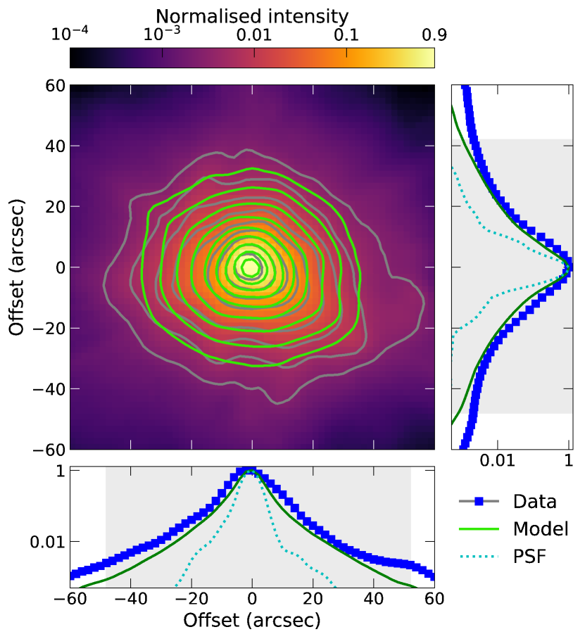
Figure 1: Observed (colour scale and grey contours) and model (green contours, see Section 3) 70 µm maps of AFGL 2591. Contour levels, in intensity normalised to peak value (87.3 Jy), are $5,10,20...1280\times\sigma_{\rm rms}$ with $\sigma_{\rm rms}=50$ mJy. Bottom and right panels show a slice through the peak in the horizontal and vertical directions, respectively. The blue squares in the side panels correspond to the observations (errors are smaller than the point size), the green continuous line is the best-fitting model presented in Section 4 and the dotted cyan line is the PSF. The shaded region enclose the points higher than $5\sigma_{\rm rms}$.

2.2 NOEMA 1.3 mm observations

AFGL 2591 was observed in the 1.3 mm spectral band with NOEMA between August 2014 and February 2016 as part of the CORE project (Beuther et al., 2018). The observations were undertaken in three array configurations (A, B, and D) at 1.37 mm with the wide-band correlator Widex and a narrow-band correlator (for a complete overview of the spectral setup see Ahmadi et al., 2018). The data were reduced by the CORE team and continuum visibilities were extracted and then CLEANed (see Beuther et al., 2018). To facilitate the comparison between models and observations, we separate the analysis of the A+B visibilities, or extended configurations, and the D visibilities, or compact configuration. For the purpose of this paper we use the continuum data from A+B and D configurations, and only the compact configuration for the CH₃CN molecular line data in order to analyse the kinematics of the inner envelope ($<10000$ au scales). A study of the CH₃CN chemistry using the combined A+B+D data can be found in Gieser et al. (2019). The study of the kinematics of the disc (if any) from the combined data set will be the focus of future publications (e.g. Ahmadi et al. in prep.).

The beam size of the compact configuration continuum observations is $2\aas@@fstack{\prime\prime}3\times 1\aas@@fstack{\prime\prime}6\;{\rm PA}=88\aas@@fstack{\circ}7$, whilst the beam size of the combined extended configurations is $0\aas@@fstack{\prime\prime}48\times 0\aas@@fstack{\prime\prime}38\;{\rm PA}=56\degr$. Vector-averaged radial visibility profiles were extracted, where we used the standard error of the mean of the points in each uv-distance bin as measure of the errors. The profiles are shown in Fig. 2 whilst the CLEAN images are shown in Fig. 3. The NOEMA/CORE A+B observations recover more emission towards smaller baselines than previous PdBI 1.4 mm A+B observations by Wang et al. (2012) after taking into consideration the difference in wavelengths, whilst achieving similar angular resolution.

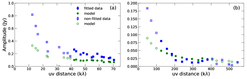
Figure 2: NOEMA 1.3 mm observed (blue squares) and simulated (green circles, see Section 3) interferometry visibility profiles. (a) Compact (D) configuration visibility profile. (b) Extended (A+B) configurations visibility profile. The selection of the data to be fitted is explained in Appendix C (online).

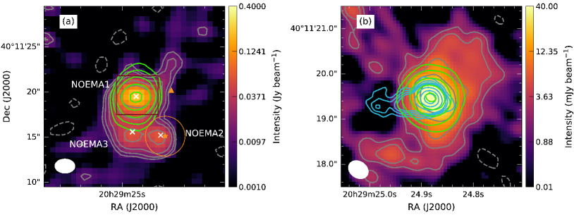
Figure 3: NOEMA 1.3 mm observed (colour scale and grey contours) and model (green contours, see Section 3) CLEAN images. The compact configuration map is shown in (a) and the levels are $-2,2,3,5,10,20\times\sigma_{\rm rms}$ with $\sigma_{\rm rms}=5.0$ mJy beam^-1. The white crosses mark the position of the continuum sources in Table 3. The orange star and circle show the position and 3.6 cm deconvolved size (${\sim}4.4$ arcsec; Johnston et al., 2013) of VLA 1. The orange triangle shows the position of VLA 2. The extended configurations map is shown in (b) and the levels are $-3,3,5,10,20,40\times\sigma_{\rm rms}$ with $\sigma_{\rm rms}=0.8$ mJy beam^-1. For comparison, the VLA 3.6 cm observations of Johnston et al. (2013) are plotted in light blue contours at $3,4,5,7,10,15,20\times\sigma_{\rm rms}$ levels with $\sigma_{\rm rms}=30\,\mu$Jy beam^-1. The dark red square in (a) shows the area covered in (b). The observed beam is shown in the bottom left corner.

The methyl cyanide CH₃CN $J=12-11$ line was covered by the narrow-band correlator with a spectral resolution of 0.312 MHz (0.43 km s^-1). A data cube covering the transition’s $K$-ladder between $K=0-5$ was extracted. The beam size of these observations is $2\aas@@fstack{\prime\prime}6\times 1\aas@@fstack{\prime\prime}8\;{\rm PA}=87\degr$. The average noise measured in an annulus of sky along all channels is $\sigma_{\rm rms}=30$ mJy beam^-1 per channel, with variations between $10-50$ mJy beam^-1 at different channels.

Zeroth- and first-order moment maps for the transition with $K=3$ are shown in Fig. 4. The first moment maps were calculated considering all data with fluxes larger than $5\sigma_{\rm rms}=0.15$ Jy beam^-1 per channel over a range of spectral channels covering the lines. The local standard of rest (LSR) velocity measured by Kaźmierczak-Barthel et al. (2014, $-5.5\pm 0.5$ km s^-1) over 24 lines in Herschel/HIFI observations was used to shift the velocities, so zero velocity corresponds to the line systemic velocity.

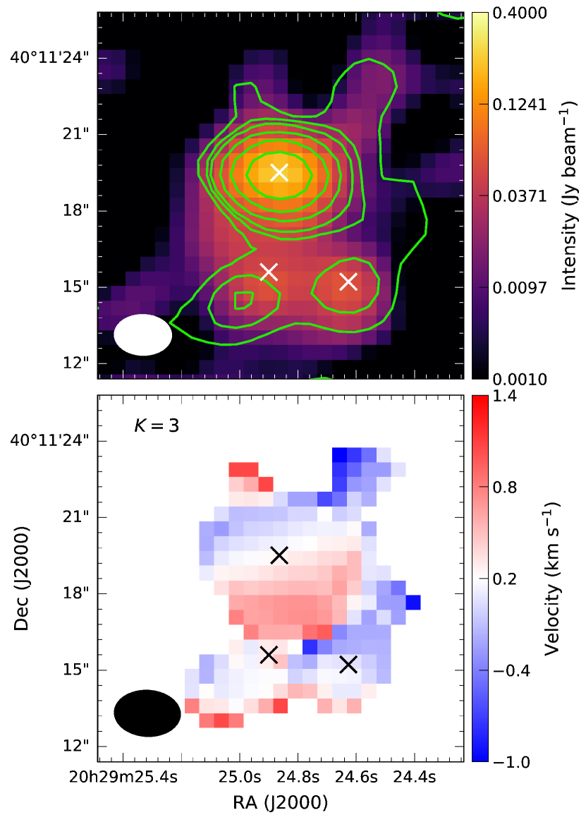
Figure 4: NOEMA compact configuration zeroth (upper row) and first (lower row) moment maps of CH₃CN $J=12-11$ for the $K=3$ transition. The continuum is plotted in colour scale in the zeroth moment maps. The zeroth moment contour levels are $1,3,5,10,20,40\times\sigma_{\rm rms}$ with $\sigma_{\rm rms}=0.45$ Jy beam^-1 km s^-1. Zero velocity correspond to the systemic velocity in the LSR system ($v_{\rm LSR}=-5.5$ km s^-1). The positions of the continuum sources are marked with a cross and the beam size is shown in the bottom left corner.

We identified 3 continuum sources from the compact configuration data named NOEMA 1–3 and their positions and peak intensities are summarised in Table 2. The position of NOEMA 1 is consistent with the VLA 3 source, for consistency to previous works we will use the latter name. Fig. 3(a) reveals the presence of at least 2 sources south of VLA 3. Thus, the NOEMA images (continuum and zeroth moment compact configuration maps) were fitted with three 2-D Gaussian components and the results are listed in Table 3. The observed size of VLA 3 decreases slightly with increasing $K$ transition, i.e. decreases with increasing upper energy of the line, and the source is only partially resolved by the molecular line observations. The orientation of the source from the methyl cyanide emission seems to agree with the large-scale orientation of the near-IR images, but the beam is oriented in the same direction. In fact, the deconvolved PAs shown in Table 4 have large uncertainties, thus the orientation is strongly affected by the beam.

Table 2: Summary of NOEMA compact configuration continuum sources.

NOEMA	VLA	RA	Dec	Peak flux
Source	Source	(J2000)	(J2000)	(mJy beam-1)
1	3	20 29 24.864	40 11 19.51	230
2	1	20 29 24.627	40 11 15.22	62
3	–	20 29 24.900	40 11 15.60	61

Similarly, a single 2-D Gaussian was fitted to the extended configurations emission in Fig. 3(b). The results listed in Table 3 show that the position angle of the emission is closer to perpendicular to the radio jet in Fig. 5 (${\sim}100\degr$, Johnston et al., 2013) rather than oriented in the outflow direction. Although the Gaussian fit is just an approximation, the orientation of the lower level contours in Fig. 3(b) shows a similar orientation.

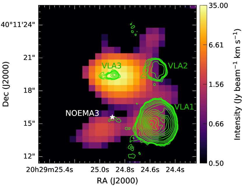
Figure 5: VLA 3.6 cm continuum emission (green contours) from Johnston et al. (2013) superimposed to the NOEMA compact configuration CH₃CN $J=12-11$ $K=3$ zeroth moment map (colour scale). Sources are labelled and the position of the continuum source NOEMA 3 is marked with a white star. Following Johnston et al. (2013), contours are 3, 4, 5, 7, 10, 15, 20, 30–100$\times\sigma_{\rm rms}$ ($\sigma_{\rm rms}=30\,\mu$Jy beam^-1).

Table 3: Measured properties from 2-D Gaussian fit to the NOEMA 1.3 mm continuum and CH₃CN zeroth-order moment emission.

$K^{a}$	Frequency	$E_{u}^{a}$	RA	Dec	Peakb	$T_{\rm B}^{c}$	Fluxd	Major	Minor	PA
	(GHz)	(K)	(hh:mm:ss)	(°:’:")		(K)		(arcsec)	(arcsec)	(deg)
NOEMA 1 (VLA 3)
Continuum (compact)			20 29 24.864	40 11 19.51	210$\pm$6	–	436$\pm$12	3.28$\pm$0.04	2.37$\pm$0.06	267$\pm$2
Continuum (extended)			20 29 24.875	40 11 19.46	50$\pm$3	–	180$\pm$11	0.90$\pm$0.05	0.72$\pm$0.03	21$\pm$9
0	220.74726	68.87	20 29 24.864	40 11 19.41	32.7$\pm$0.6	40.9	39.3$\pm$0.7	2.87$\pm$0.03	2.04$\pm$0.05	87.1$\pm$0.9
1	220.74301	76.01	20 29 24.861	40 11 19.38	26.4$\pm$0.5	37.9	31.6$\pm$0.6	2.85$\pm$0.03	2.04$\pm$0.05	86.8$\pm$1.0
2	220.73026	97.44	20 29 24.861	40 11 19.39	24.5$\pm$0.6	34.5	28.9$\pm$0.7	2.82$\pm$0.04	2.03$\pm$0.06	86.1$\pm$1.3
3	220.70902	133.16	20 29 24.861	40 11 19.39	32.1$\pm$0.6	53.9	37.8$\pm$0.7	2.81$\pm$0.04	2.03$\pm$0.05	84.7$\pm$1.1
4	220.67929	183.15	20 29 24.861	40 11 19.36	16.2$\pm$0.4	22.3	18.3$\pm$0.5	2.81$\pm$0.05	1.96$\pm$0.07	84.6$\pm$1.3
5	220.64108	247.40	20 29 24.856	40 11 19.36	12.4$\pm$0.3	15.3	13.7$\pm$0.4	2.86$\pm$0.05	1.93$\pm$0.07	87.7$\pm$1.3
NOEMA 2
Continuum (compact)			20 29 24.627	40 11 15.22	48$\pm$6	–	76$\pm$9	2.9$\pm$0.3	2.0$\pm$0.2	18$\pm$7
0	220.74726	68.87	20 29 24.62	40 11 15.5	2.3$\pm$0.3	2.7	3.8$\pm$0.5	3.2$\pm$0.3	2.6$\pm$0.3	137$\pm$14
1	220.74301	76.01	20 29 24.62	40 11 15.5	1.9$\pm$0.3	3.3	3.3$\pm$0.4	3.1$\pm$0.3	2.7$\pm$0.3	140$\pm$15
2	220.73026	97.44	20 29 24.62	40 11 15.6	1.6$\pm$0.3	2.3	3.4$\pm$0.5	3.5$\pm$0.4	3.0$\pm$0.3	151$\pm$17
3	220.70902	133.16	20 29 24.63	40 11 15.4	2.1$\pm$0.3	2.9	4.1$\pm$0.6	3.4$\pm$0.4	2.8$\pm$0.3	136$\pm$15
4	220.67929	183.15	20 29 24.63	40 11 15.5	1.0$\pm$0.2	1.3	2.1$\pm$0.3	3.7$\pm$0.4	2.8$\pm$0.3	2.7$\pm$9.5
5	220.64108	247.40	20 29 24.63	40 11 15.4	1.2$\pm$0.1	1.1	2.0$\pm$0.2	3.2$\pm$0.2	2.6$\pm$0.3	110$\pm$9
NOEMA 3
Continuum (compact)			20 29 24.90	40 11 15.6	57$\pm$6	–	250$\pm$25	4.9$\pm$0.2	3.3$\pm$0.2	49$\pm$5
0	220.74726	68.87	20 29 24.99	40 11 14.5	2.6$\pm$0.3	2.8	3.2$\pm$0.3	3.2$\pm$0.2	1.9$\pm$0.3	114$\pm$4
1	220.74301	76.01	20 29 24.99	40 11 14.5	2.1$\pm$0.2	3.1	2.8$\pm$0.3	3.2$\pm$0.2	2.0$\pm$0.2	113$\pm$4
2	220.73026	97.44	20 29 24.99	40 11 14.5	2.1$\pm$0.3	2.9	2.3$\pm$0.3	2.9$\pm$0.3	1.8$\pm$0.3	117$\pm$6
3	220.70902	133.16	20 29 24.98	40 11 14.5	2.5$\pm$0.3	3.4	3.2$\pm$0.4	3.3$\pm$0.2	1.9$\pm$0.3	110$\pm$4
4	220.67929	183.15	20 29 24.98	40 11 14.4	1.5$\pm$0.3	1.4	1.7$\pm$0.3	3.0$\pm$0.3	1.8$\pm$0.4	111$\pm$6
5	220.64108	247.40	20 29 24.97	40 22 14.6	1.0$\pm$0.2	1.3	1.2$\pm$0.2	3.2$\pm$0.3	1.8$\pm$0.4	110$\pm$6

Notes. The 2-D Gaussian components were fitted simultaneously to the continuum images, whilst for the methyl cyanide zeroth moment maps each source was fitted separately within a box isolating each source.

^a From Leiden Atomic and Molecular Database (LAMDA).

^b The units of peak fluxes are mJy beam^-1 for the continuum observations and Jy beam^-1 km s^-1 for the molecular lines.

^c Brightness temperature at the line peak at the position of the zeroth moment peak.

^d The units of flux are mJy for the continuum observations and Jy km s^-1 for the molecular lines.

Table 4: Deconvolved 2-D Gaussian fit sizes for NOEMA 1 (VLA 3) from NOEMA compact configuration CH₃CN emission at different $K$ transition.

$K$	Major	Minor	PA
	(arcsec)	(arcsec)	(deg)
0	1.14$\pm$0.08	0.86$\pm$0.12	87$\pm$175
1	1.09$\pm$0.09	0.88$\pm$0.13	83$\pm$173
2	1.00$\pm$0.13	0.84$\pm$0.19	73$\pm$79
3	1.01$\pm$0.13	0.80$\pm$0.18	58$\pm$41
4	1.00$\pm$0.17	0.61$\pm$0.37	69$\pm$31
5	1.12$\pm$0.14	0.55$\pm$0.43	90$\pm$176

To extract the kinematic information from the observations of VLA 3, we calculated position-velocity (pv) maps for CH₃CN lines with $K=2-5$ and are shown in Fig. 6. The slices were obtained at 6° (along the putative disc major axis from Wang et al., 2012) and 276° (along the outflow direction; see online Appendix C for a discussion) with a slice width of 1.8 arcsec (3 times the pixel size and close to the beam width).

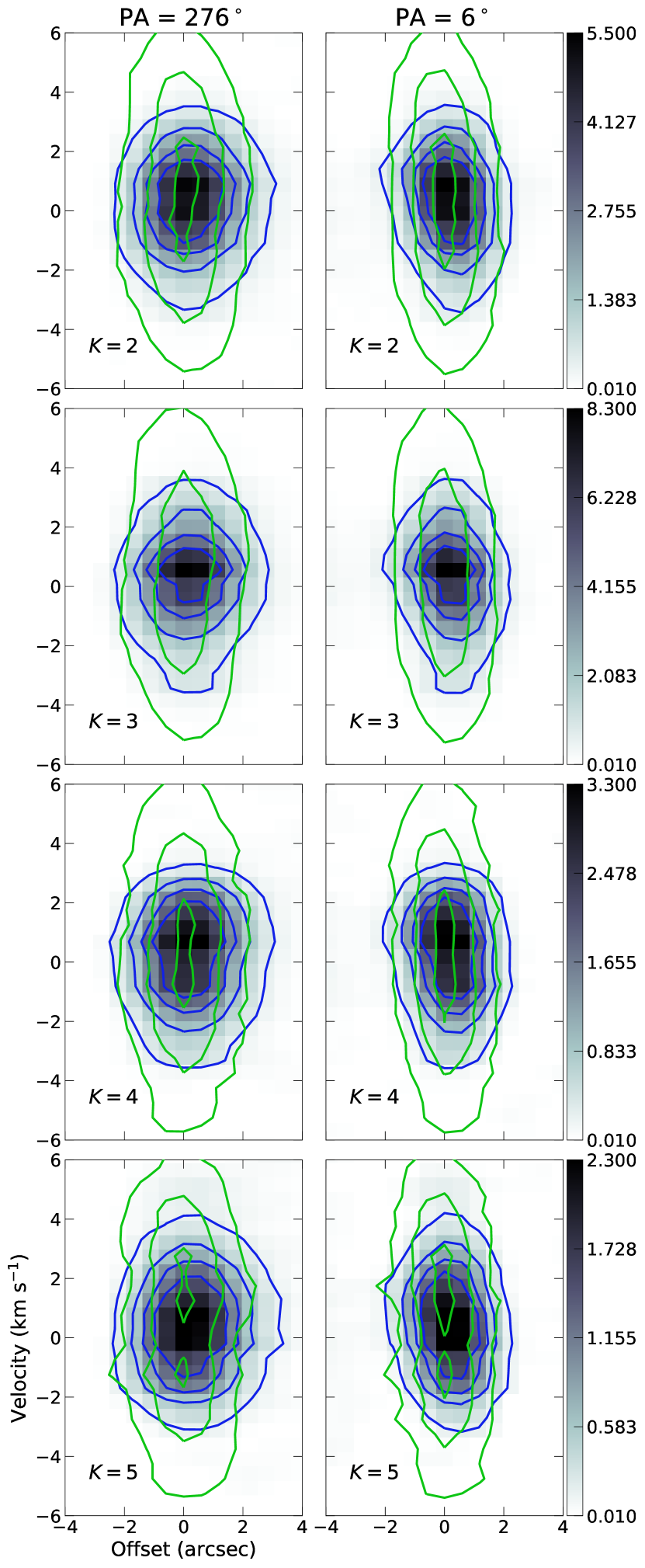
Figure 6: Observed position-velocity (pv) maps (grey scale and blue contours) and best-fitting model pv maps (green contours, see Section 3) of the CH₃CN $J=12-11$ $K=2-5$ line emission for a position angle of 276° (left column), i.e. along the rotation axis, and 6° (right column). Contours levels are 10–80 per cent in 20 per cent steps of 5, 8, 3 and 2 Jy beam^-1 for each $K$ line, respectively.

The position of NOEMA 2 is close to VLA 1 and its total flux (${\sim}0.1$ mJy) is consistent with the value predicted from the VLA 1 radio spectral index ($\alpha=0$, Johnston et al., 2013). In Fig. 5, it can be seen that the methyl cyanide emission of NOEMA 2 coincides with emission from the eastern hemisphere of VLA 1. This is consistent with VLA 1 being a slightly cometary H ii region with the ionising gas expanding towards the less dense gas in the west.

The source immediately south of VLA 3, NOEMA 3, has an intensity peak which is shifted ${\sim}4$ arcsec towards the south east from the continuum peak of VLA 3. This source is not associated with 3.6 cm radio continuum emission above a level of $3\sigma=90$ $\mu$Jy beam^-1 (see Fig. 5) and has not been detected in the IR, thus its nature is as yet unknown. Fig. 4 also shows that the velocity structures of the three sources can be separated from each other.

2.3 Other continuum multi-wavelength data

Multi-wavelength observations were used to constrain the dust density and temperature distributions. Since these images were previously processed, only the sky level was subtracted when necessary. Table 5 presents a summary of the observations which were used to extract spatial information for the fitting and are described below.

Table 5: Summary of continuum observations used to extract spatial information.

$\lambda$	Instrument	Resolution	Typea
(µm)
1.2	UKIRT/WFCAM	0$\aas@@fstack{\prime\prime}$9	I
1.6	UKIRT/WFCAM	0$\aas@@fstack{\prime\prime}$9	I
2.1	UKIRT/WFCAM	0$\aas@@fstack{\prime\prime}$9	I
2.1	SAO/6 m	0.17″	V
70	Herschel/PACS	$6\aas@@fstack{\prime\prime}51\times 5\aas@@fstack{\prime\prime}44$	I
450	JCMT/SCUBA	9″	P
850	JCMT/SCUBA	14″	P
1300	NOEMA (D)	$2\aas@@fstack{\prime\prime}3\times 1\aas@@fstack{\prime\prime}6$ PA $88\aas@@fstack{\circ}7$	V
1300	NOEMA (A+B)	$0\aas@@fstack{\prime\prime}48\times 0\aas@@fstack{\prime\prime}38$ PA $56\degr$	V

^a Type of data product used to compare observations and models: I for images, V for visibility profiles and P for azimuthally averaged radial profiles.

2.3.1 Near-IR imaging

Near-IR images from the UKIRT Wide Field Camera (WFCAM, Casali et al., 2007) at 1.2, 1.6 and 2.1 µm, $J$, $H$ and $K$ bands respectively, were obtained from the UKIRT Infrared Deep Sky Survey (UKIDSS; Lucas et al., 2008) and are presented in Fig. 7. These data have higher resolution (${\sim}1$ arcsec) than the 2MASS data used by Johnston et al. (2013), which had a resolution of ${\sim}2.5$ arcsec. The images were flux-calibrated and error maps were obtained by using Poisson statistics on the un-calibrated data converted to counts. A Moffat function was fitted to several saturated and unsaturated nearby point-like sources to produce a PSF image. This function has been proven reliable in reproducing the PSF wings (e.g. McDonald et al., 2011). The core of saturated sources were masked in order to fit better the PSF wings. The FWHM of the fitted Moffat function are $0.9\pm 0.1$, $0.9\pm 0.2$ and $0.9\pm 0.2$ arcsec and the atmospheric scattering coefficients are $3.0\pm 0.4$, $2.7\pm 0.4$ and $2.7\pm 0.7$ for the $J$, $H$ and $K$-bands, respectively. These widths are consistent with the observed seeing FWHM of 0.8 arcsec, as recorded in the header of the images.

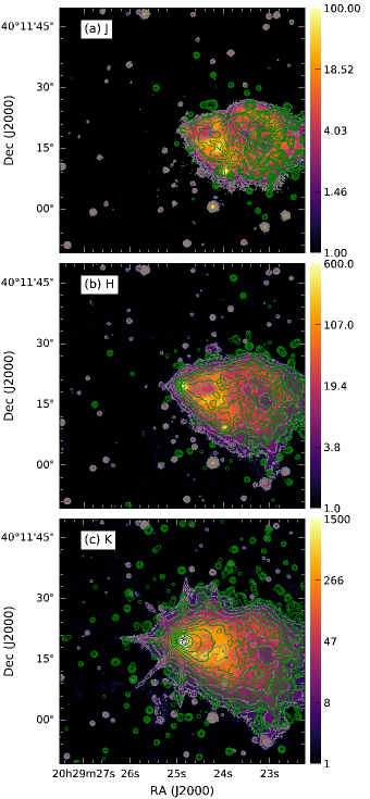
Figure 7: Observed (colour map and grey contours) and model (green contours, see Section 3) near-IR maps of AFGL 2591. The $J$-band data and model are shown in (a) and contour levels are $3,5,10,20,40\times\sigma_{\rm rms}$ with $\sigma_{\rm rms}=0.3$ MJy sr^-1. (b) shows the $H$-band data and model in contours at levels $5,10,20-160\times\sigma_{\rm rms}$ with $\sigma_{\rm rms}=0.4$ MJy sr^-1. (c) shows the $K$-band data and model in contours at levels $5,10,20-2560\times\sigma_{\rm rms}$ with $\sigma_{\rm rms}=0.6$ MJy sr^-1. The colour maps are in units of MJy sr^-1.

In order to study the regions close to the MYSO, which are saturated in the UKIRT images, we used Special Astrophysical Observatory (SAO) 6 m telescope $K$-band speckle interferometric visibilities from Preibisch et al. (2003). The visibilities were averaged over annuli with constant width and the standard deviation of the data in each annulus was used as a measure of the errors. Fig. 8 shows the visibility radial profile. It is worth noticing that the visibilities are reasonably symmetric which results in relatively small errors (see Preibisch et al., 2003, their fig. 2).

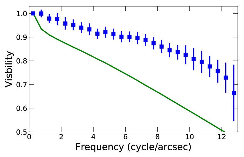
Figure 8: $K$-band speckle interferometry visibilities radial profile. Observed points are represented by blue squares and the best-fitting model by a continuous green line. The model clearly underestimates the observations (see Section 4.1).

2.3.2 (Sub)mm

In the submm, images were obtained from the JCMT Legacy Catalogue (Di Francesco et al., 2008) which were taken with SCUBA at 450 and 850 µm. Following Di Francesco et al. (2008), we prepared a PSF composed of two Gaussians which reproduce the main and secondary lobes. The main lobes have a FWHM of 9 and 14 arcsec at 450 and 850 µm respectively, whilst 2-D Gaussians fitted to observed emission towards AFGL 2591 have a FWHM of $37\aas@@fstack{\prime\prime}1\times 28\aas@@fstack{\prime\prime}5\;{\rm PA}=247\degr\pm 1\degr$ and $47\aas@@fstack{\prime\prime}6\times 38\aas@@fstack{\prime\prime}7\;{\rm PA}=233\degr\pm 1\degr$ respectively. Hence the source is elongated with position angles of the 2-D Gaussian major axis consistent with the outflow cavity direction, as in the 70 µm data. However, since the real PSF is known to be more complicated and changes between nights (e.g. Hatchell et al., 2000), we fit azimuthally averaged radial intensity profiles (hereafter radial intensity profiles). The radial intensity profiles shown in Fig. 9 were calculated as the average flux of concentric annuli regions of constant width and their errors are the standard deviation of the enclosed fluxes.

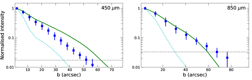
Figure 9: Normalised radial intensity profiles at 450 and 850 µm. Observed profiles are represented with blue squares and the best-fitting model by a green continuous line (see Section 3). The horizontal dotted line represents the $3\sigma$ level above zero, where $\sigma$ is the noise level. Observed points above this level were compared with the model ones. The cyan dotted line shows the PSF profile.

2.3.3 Spectral energy distribution

The spectral energy distribution (SED) consists of data points from Johnston et al. (2013) for $\lambda<60$ µm and the data points in Table 6 for longer wavelengths. The whole SED is shown in Fig. 10. The fluxes for the Herschel bands, observed by PACS and the Spectral and Photometric Imaging Receiver (SPIRE, Griffin et al., 2010), were obtained from the sum of all pixels with intensity higher than three times the image noise. This filters out the filamentary emission observed in SPIRE data whilst the fluxes are within the calibration uncertainties of the ones calculated with an aperture covering the whole region. The flux calibration uncertainties for PACS and SPIRE in the literature range from ${\sim}5$ to 15 per cent (e.g. Sadavoy et al., 2013; Roy et al., 2014, and Herschel online documentation). We adopted an uncertainty of 10 per cent for both.

Table 6: SED data points for $\lambda\geqslant 60$ µm.

Wavelength	Flux	Instrument	Ref.
(µm)	(Jy)
70	$5600\pm 560$	Herschel/PACS	(1)
160	$4055\pm 406$	Herschel/PACS	(1)
250	$1250\pm 125$	Herschel/SPIRE	(1)
350	$426\pm 43$	Herschel/SPIRE	(1)
450	$222\pm 110$	JCMT/SCUBA	(2)
500	$123\pm 12$	Herschel/SPIRE	(1)
850	$26.8\pm 5.2$	JCMT/SCUBA	(2)
1200	$8.1\pm 0.8$	IRAM 30m/MAMBO	(3)

(1) This work. Data from PACS and SPIRE were obtained from the HOBYS observations, with SPIRE data from high gain dedicated observations.

(2) Di Francesco et al. (2008)

(3) Roy et al. (2011) based on Motte et al. (2007)

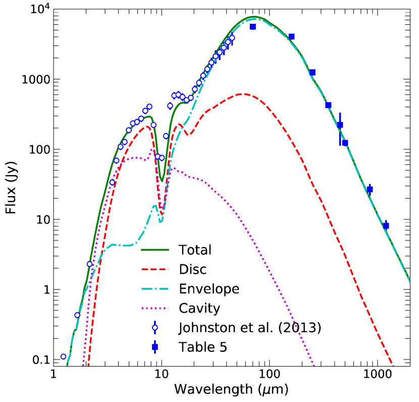
Figure 10: SED of AFGL 2591 and the best-fitting model. The emission from each of the different components included in the model are also shown (see legend).

3 Data modelling

3.1 Multi-wavelength data modelling

We performed a radiative transfer modelling of the multi-wavelength dust continuum and CH₃CN observations to obtain density, temperature and velocity distributions. The fit was performed in 3 steps and is described in Fig. 11(a). Each step involved the production of synthetic observations as described in Fig. 11(b) to obtain the model data products (images, intensity radial profiles, etc.) which were then compared with the observations. To produce synthetic data, we used the 3-D radiative transfer codes hyperion (Robitaille, 2011) for dust continuum and mollie (Keto & Rybicki, 2010) for line emission. The modelling steps included one visual inspection for the continuum fitting and model grid fitting for some continuum observations and the CH₃CN observation. Details and the particularities of the modelling and synthetic observations are described in Appendices A–C (online).

Figure 11: Radiative transfer modelling procedure. (a) Overall procedure. The blue dashed boxes show the 2 steps followed to fit the dust continuum data, whilst the grey dashed box shows the procedure used to fit the CH₃CN molecular line emission observations. Purple circles involve performing radiative transfer steps. (b) Image processing procedure performed at the end of each radiative transfer computation. Green boxes represent final products of each step. Detail descriptions of the procedures and additional tables are available in the online Appendices.

3.2 1-D LTE and non-LTE CH₃CN modelling

We fitted the methyl cyanide 12–11 $K$-ladder with the program cassis to study some physical properties of the gas (e.g. temperature). This program uses a Markov chain Monte Carlo (MCMC) which samples the parameter space in order to minimise the $\chi^{2}$ between the observed and synthetic spectra. We used one isothermal density component model to fit the observations and their parameter ranges are listed in Table 7. cassis calculates spectra under the LTE approximation, or the non-LTE approximation by using the radiative transfer code radex (van der Tak et al., 2007). Two density component models were experimented upon, but similar results were obtained.

Table 7: Parameter constraints of the modelling with cassis.

Parameter	Limits
Column density ($N_{\rm CH_{3}CN}$)	$10^{13}-10^{18}$ cm-2
H2 density ($n_{\rm H_{2}}$)a	$10^{3}-10^{9}$ cm-3
Excitation temperature ($T_{\rm ex}$)	10–500 K
Size	0–1.2 arcsec
Line width ($\Delta v$)	1–7 km s-1
Offset to LSR velocity ($\Delta v_{\rm LSR}$)b	-2–2 km s-1

^a Only for the non-LTE case.

^b $v_{\rm LSR}=-5.5$ km s^-1.

In order to limit the region to analyse, only spectra with at least one line with a flux higher than 0.25 Jy beam^-1 (${>}5\sigma$) were considered in the fit. Additionally, cassis requires an estimate of each line rms and the flux calibration error. The first was estimated from boxes around the lines and vary between 0.04–0.06 K, where the higher the K line the higher the error. The relative flux calibration error was fixed to 20 per cent (Beuther et al., 2018).

The size parameter in Table 7 is the source size and is used to calculate the beam dilution factor, which is defined in cassis as

$$\Omega=\frac{\theta^{2}}{\theta^{2}+\theta_{\rm B}^{2}}\,,$$ (1)

where $\theta$ is the source size and $\theta_{\rm B}$ is the beam size derived from the configuration files specific for each telescope, which include its diameter/largest baseline. In this case, the baseline used was calculated to match the resolution of the observations. The brightness temperature is then calculated by cassis as

$$T_{b}=\Omega J_{\nu}(T_{\rm ex})(1-e^{-\tau})+f({\rm CMB,dust})\,,$$ (2)

where $J_{\nu}(T_{\rm ex})=h\nu k^{-1}(e^{h\nu/kT_{\rm ex}}-1)^{-1}$, $T_{\rm ex}$ is the excitation temperature, $\tau$ is the line optical depth and $f({\rm CMB,dust})$ accounts for the contribution from the cosmic microwave background and dust emission.

4 Results

4.1 Continuum modelling

The parameters of the overall best-fitting model, i.e. after the continuum grid fitting step, are listed in Table 8. The extended emission observed at 70 µm is relatively well fitted by the best-fitting model up to ${\sim}40$ arcsec from the centre as shown in Fig. 1. In general, the model matches the elongation in the data. At 1 per cent of the peak intensity, where the model has a better fit, the horizontal slice, which cuts through the cavity, is more elongated than the vertical one in the model and the observations as listed in Table 1. This cannot be explained by any asymmetry in the 70 µm PSF, which is relatively symmetric as shown in the same table. Fig. 12 shows the 70 µm image before convolution with the PSF, where the contribution of the cavity to the elongation can be observed. The emission is underestimated close to the source and along the cavity axis (PA$=259\degr$, see Fig. 1). As a result, the angular sizes of the model at the FWHM from slices and 2-D Gaussian fit listed in Table 1 are similar between each direction.

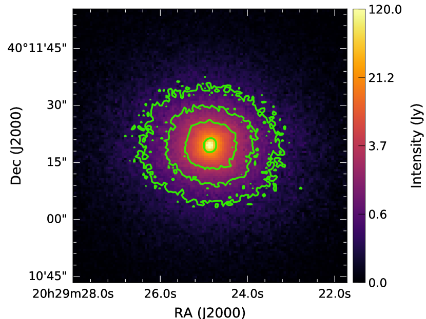
Figure 12: Unprocessed model image of the best-fitting model at 70 µm. Contour levels are 0.1, 0.3, 1 and 10 per cent of the peak intensity. Note the elongation along the cavity axis oriented at PA$=259\degr$ as the distance to the source increases.

The parameters of the best-fitting model during the visual inspection step are listed in Table 8 and the ranking and reduced $\chi^{2}$ values for each observation are listed in Table 9. The best-fitting model has a type A density distribution (Ulrich, 1976 envelope and a flared disc). The envelope radius was well-fitted during this step and has a value roughly a factor 1.4 smaller than the initial visual inspection model and has a similar size to the model with disc of Johnston et al. (2013). The disc scale height is smaller by roughly one order of magnitude than those in Johnston et al. (2013), but this parameter cannot be constrained by our observations, thus it was less explored. The shape of the cavity changed from the initial exponent of 1.5 to 2.0, and its reference density decreased a ${\sim}15$ per cent from its initial value and its density exponent did not change.

Table 8: Parameters of the continuum and CH₃CN line best-fitting model, which consists of an Ulrich envelope and a flared disc.

Parameter	Visual	Grid	Constrained by
	inspection
Continuum
Distance (kpc)	3.3$\pm$0.1		Fixed
Position angle (PA)	259°		Fixed
Inclination angle ($i$)	40°	$25\degr\pm 5\degr$	SED + near-IR
Stellar temperature ($T_{\star}$/K)	20000	18000	–
Stellar luminosity ($L_{\star}/10^{5}$ L☉)	1.6	$1.6\pm 0.2$	SED
Inner radius ($R_{\mathrm{in}}$/au)	36	35	SED + Speckle
Outer radius ($R_{\mathrm{out}}$/au)	195000	195000	Submm
Envelope infall rate ($\dot{M}_{\mathrm{env}}/10^{-3}\,\mbox{M${}_{\sun}$}\,{\rm yr}^{-1}$)	1.1	$2.0\pm 0.2$	SED + (sub)mm
Envelope dust	OHM92		–
Centrifugal radius ($R_{\mathrm{c}}$/au)	200	$2200\pm 200$	NOEMA ext.
Disc mass ($M_{\mathrm{d}}$/M☉)	1.0	$6\pm 1$	NOEMA ext.
Disc scale height at $r=100$ au ($h_{0}$/au)	0.6		–
Disc flaring exponent ($\alpha$)	1.88	2.25	–
Disc vertical density exponent ($\beta$)	1.13	1.25	–
Disc dust	OHM92		–
Cavity opening anglea ($2\theta_{\rm cav}$)	60°	$60\degr\pm 5\degr$	Near-IR + SED
Cavity shape exponent ($b_{\mathrm{cav}}$)	2.0		Near-IR + SED
Cavity density exponent ($p_{\rm cav}$)	2.0		Near-IR + SED
Cavity reference densitya ($\rho_{\rm cav}/10^{-21}$ g cm-3)	1.4		Near-IR + SED
Cavity dust	KMH		–
Extra parameters for line emission
Position angle (PA)	–	276°	Fixed
Stellar mass ($M_{\star}/\mbox{M${}_{\sun}$}$)	–	35	Fixed
Abundance for $T>100$ K ($X_{1}$)	–	$2\times 10^{-8}$	–
Turbulent width ($\Delta v_{\rm nth}/{\rm km\,s}^{-}1$)	–	2	–
Outflow velocitya ($v_{0}/{\rm km\,s}^{-}1$)	–	0, 1b	–

Notes. Parameters in bold under the last column are the 10 free parameters that can be constrained by the observations. The inner radius depends on the stellar luminosity.

^a Defined at a height $z=10^{4}$ au.

^b 2 models had the same best overall ranking value.

Table 9: Overall ranking and reduced $\chi^{2}$ values for the continuum best-fitting models of each type.

Type	Ranka	70 µm	SED	$J$	$H$	$K$		450 µm	850 µm	1.3 mm		$\chi^{2}$	$\langle\chi^{2}\rangle$
						UKIRT	Speckle			extended	compact
Overall best-fitting model
A	–	211	7.0	26	64	316	32	13	0.40	408	557	–	–
Best-fitting model by density type
A	662	114	9.7	23	79	311	49	20	0.56	993	852	137	164
B	854	160	7.3	25	81	305	35	17	0.51	1040	1142	137	194
C	1019	305	44.1	21	107	523	469	3	0.10	557	300	217	175
Best-fitting model by $\chi^{2}$
A	1134	100	8.9	26	91	223	44	45	3.60	926	1570	113	160
Best-fitting model by $\langle\chi^{2}\rangle$
C	1278	274	54.2	23	155	624	25	0.7	1.16	156	195	267	125

^a Average weighted ranking as described in Appendix A.1.2 (online).

Similarly, in Table 8 and 9 we list the results for the overall best-fitting model after the grid fitting step. The disc mass and radius increased with respect to the visual inspection best-fitting model. The former is roughly a third of the disc mass in the control model of Johnston et al. (2013), but the disc radii are similar. This difference is explained by the difference in the disc scale height. The cavity opening angle is equal to the one from the visual inspection best-fitting model, and the inclination angles differ by 15°. The luminosities are the same between the best-fitting models at each step, whilst the envelope infall rate is ${\sim}1.8$ times higher in the overall best-fitting model.

The model SED agrees reasonably well with the observations as shown in Fig. 10. The total mass of the model, $M=2.1\times 10^{3}$ M_☉, is enough to fit the 10 µm silicate feature relatively well at an inclination of 25° and closely fit the submm points. This is 900 M_☉ more massive than the model with disc of Johnston et al. (2013), but 600 M_☉ less massive than their envelope only model. Models with WD01 dust can also fit in the submm with lower masses, however they underestimate the fluxes between 3–8 µm by a factor ${\sim}10$.

The near-IR maps in Fig. 7(a)–(c) show that the near-IR band images are well reproduced. However, Fig. 8 shows that the small scales closer to the star position probed by the speckle observation are not well reproduced. In general, most models with a cavity density of the same order as the best-fitting model do not fit this observation.

At 450 µm, the best-fitting model overestimates the emission at larger scales as shown in Fig. 9. Type C models with WD01 dust are able to reproduce this profile but not the near-IR observations. At 850 µm, most of the models reproduce the radial profile relatively well. These two fits are unaffected by the inclination angle. Palau et al. (2014) successfully fitted these profiles with a spherically symmetric model and obtained a density power law index of 1.8, which is slightly lower than our type C models but steeper than the Ulrich envelope. However, an analysis of the observed images shows that the observed source is more elongated along the cavity at both wavelengths, but this is not seen in our models.

The 1.3 mm extended configuration visibilities are relatively well fitted as shown in Fig. 2(b). Models with WD01 dust or larger and more massive discs are able to match the data for baselines smaller than ${\sim}150$ k$\lambda$, but these baselines were not included in the fitting process. For longer baselines, the intensity is determined mainly by the mass of the disc, $6$ M_☉ in the best-fitting model. The best-fitting model underestimates the observed 1.3 mm compact configuration visibilities (Fig. 2a) at large spatial scales (smaller uv distances). This is observed in most models. However, those models with WD01 dust give an improvement of the fit, but they do not fit the short wavelengths ($\lambda<12$ µm) of the SED.

At ${\sim}10^{4}$ au scales, as mapped by the 1.3 mm compact configuration observations in Fig. 3(a), the model FWHM is $3\aas@@fstack{\prime\prime}2\times 3\aas@@fstack{\prime\prime}0$ PA$=325\degr\pm 2\degr$ as obtained from a 2-D Gaussian fit. This is slightly more extended than the observed size in Table 3 and has a different orientation. The presence of at least one source to the south of VLA 3, as shown in Fig. 3(a), may also contaminate the submm observations making them look more elongated than they really are. A more complete modelling of VLA 3 including the contribution of NOEMA 1 is beyond the scope of this paper.

Fig. 3(b) shows the degree of agreement between the observations and model at ${\sim}100$ au scales from the 1.3 mm extended configuration observations. It shows that the model emission is more compact than the observed one, with a FWHM of $0\aas@@fstack{\prime\prime}7\times 0\aas@@fstack{\prime\prime}6\,\mathrm{PA}=247\degr\pm 10\degr$ from a 2-D Gaussian fit (cf. Table 3). The PA of the model is closer to the orientation of the outflow cavity than to the orientation of the disc, which can be explained by the inclination angle. The extended emission in the observations also show features which cannot be explained by the model due to its symmetry.

4.1.1 Other density distributions

Table 9 lists the $\chi^{2}$ values for the best-fitting models for the different types of model densities (A, B and C) for each observation in the visual inspection fitting. The values of the parameters of the best-fitting models are listed in Table 15 (online). The best-fitting type B model has the same stellar properties as the best-fitting type A model (from grid fitting). The envelope of the best-fitting type B model has the same radius and has an infall rate $0.5\times 10^{-3}\,\mbox{M${}_{\sun}$}\,{\rm yr}^{-1}$ lower than the best-fitting type A model. The inclination angle is 10° lower than the best-fitting type A model, which may explain the better fit to the SED than the best-fitting type A from visual inspection. The distribution and shape of the cavity is the same as the best-fitting type A model. This model has an accretion luminosity of ${\sim}20$ L_☉.

The best-fitting type C model has the same inclination angle as the best-fitting type A model. It fits relatively well the submm and mm observations, but is worse at fitting the near-IR observations and the SED because its envelope has a WD01 dust. The envelope has a mass of $1.0\times 10^{3}$ M_☉ and the density in the cavity is lower ($\rho_{0,\mathrm{cav}}=3.5\times 10^{-24}$ g cm^-3) but decreases at the same rate as the best-fitting type A model. Its disc is more compact than the best-fitting type A model one from visual inspection, and slightly more massive (1.2 M_☉). In general, this type of model does not fit the 70 µm image well.

4.2 CH₃CN line modelling

4.2.1 1-D cassis modelling

We obtained similar fits to the data and results under the LTE and non-LTE approximations. The results for the LTE modelling are shown in Fig. 13. The peak column density for VLA 3 is $4.2\times 10^{16}$ cm^-2 in the LTE model, and is located at the position of the source. The average column density inside a region with radius 2 arcsec is $1.5\times 10^{16}$ cm^-2. An approximate value of the ${\rm H}_{2}$ column density can be obtained from the continuum map in the optically thin limit (e.g. Morales et al., 2009):

$$N_{{\rm H}_{2}}=\frac{S_{\nu}R_{\rm gd}}{\Omega_{\rm B}B_{\nu}(T_{\rm d})\kappa_{\nu}\mu m_{\rm H}}\,,$$ (3)

with $S_{\nu}$ the observed dust continuum flux and $\Omega_{\rm B}$ the solid angle of the beam. If eq. 3 is solved with a dust temperature $T_{\rm d}=190$ K (see below), a dust opacity $\kappa_{\rm 1.3mm}=1$ cm² g^-1, a mean molecular weight $\mu=2.3$ and a gas-to-dust ratio $R_{\rm gd}=100$, a peak ${\rm H}_{2}$ column density value of $2.0\times 10^{23}$ cm^-2 and an average of $9.9\times 10^{22}$ cm^-2 within the same 2 arcsec region are obtained. Hence the methyl cyanide abundance is $2.1\times 10^{-7}$ for the peak value and $1.5\times 10^{-7}$ for the average.

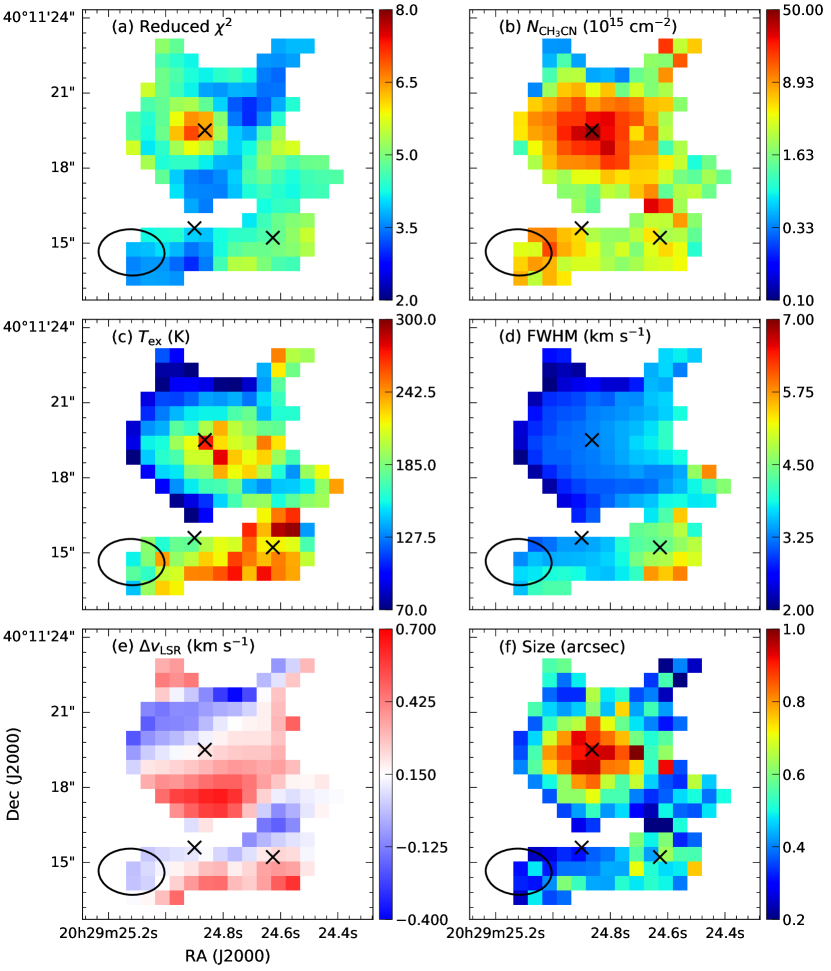
Figure 13: Results for each parameter from the 1-D LTE modelling of the NOEMA compact configuration CH₃CN $J=12-11$ transition observations. The crosses mark the position of the continuum sources in Table 3. The beam is shown in the lower left corner (black ellipse).

The excitation temperature for the LTE model in VLA 3 peaks at the source position and has a value of 271 K. In a region of radius 2 arcsec the minimum temperature is 120 K and the average is 190 K.

The FWHM of the line gets wider along the blue-shifted outflow direction. This may be due to turbulent motion of the gas in the outflow. The red-shifted outflow direction does not show the same trend, probably because the emission is optically thick towards that side. However, the fit is worse towards the red-shifted outflow direction, as shown by the reduced $\chi^{2}$ maps, hence this result should be taken with caution. The line velocity maps of VLA 3 are consistent with the first moment maps in Fig. 4.

The sizes obtained from the modelling are smaller than the beam size of the observations and the deconvolved angular size derived from continuum observations (${\sim}2.0$ arcsec from Table 3). The less beam diluted areas are located towards the denser regions. As the flux is proportional to the beam dilution factor $\Omega$ and proportional to the column density in the optically thin regime, the size and the column density parameters may be degenerate. However, if the core was spherical, the depth along the line of sight would increase towards the centre of the core.

The regions NOEMA 2 and 3 show a different temperature and velocity structure. As expected for an H ii region (VLA 1), NOEMA 2 has wider lines due to turbulent gas expansion and is hotter than the other two regions. NOEMA 2 also has a lower column density in comparison to the other two regions, which is consistent with it being optically thin at mm/radio wavelengths as found by e.g. Trinidad et al. (2003) at 3.6 cm. NOEMA 3 peaks in temperature and column density at the same position. Its peak temperature is 240 K and its column density is $1.6\times 10^{16}$ cm^-2, hence is slightly colder and less dense than VLA 3. There appears to be a similar velocity gradient in NOEMA 2 and 3 to that of VLA 3, thus there may be a common rotational motion for all the sources present.

4.2.2 3-D modelling

There are 2 best-fitting models (models with the same overall ranking), but the only difference is the outflow reference velocity. Table 8 lists the parameters of the best-fitting models for the CH₃CN $J=12-11$ $K=2$ to $K=5$ molecular line emission for a model with a stellar mass of 35 M_☉. Unless otherwise stated, we will refer to these models as the best-fitting ones as the stellar mass matches the mass derived from the source luminosity. The best-fitting models have outflow reference velocities $v_{0}=0$ and 1 km s^-1. However, this parameter may not be well constrained because the observations do not show any clear evidence of outflow motion in the first moment map, e.g. online Fig. 22. Hence for simplicity we plot the results for the model with zero outflow reference velocity. Fig. 6 shows the pv maps of the best-fitting model for each line and cut direction. The model reproduces relatively well the angular extent of the pv maps, but not the spectral extent. The zeroth moment slices in Fig. 14 also show that the angular extent is well fitted.

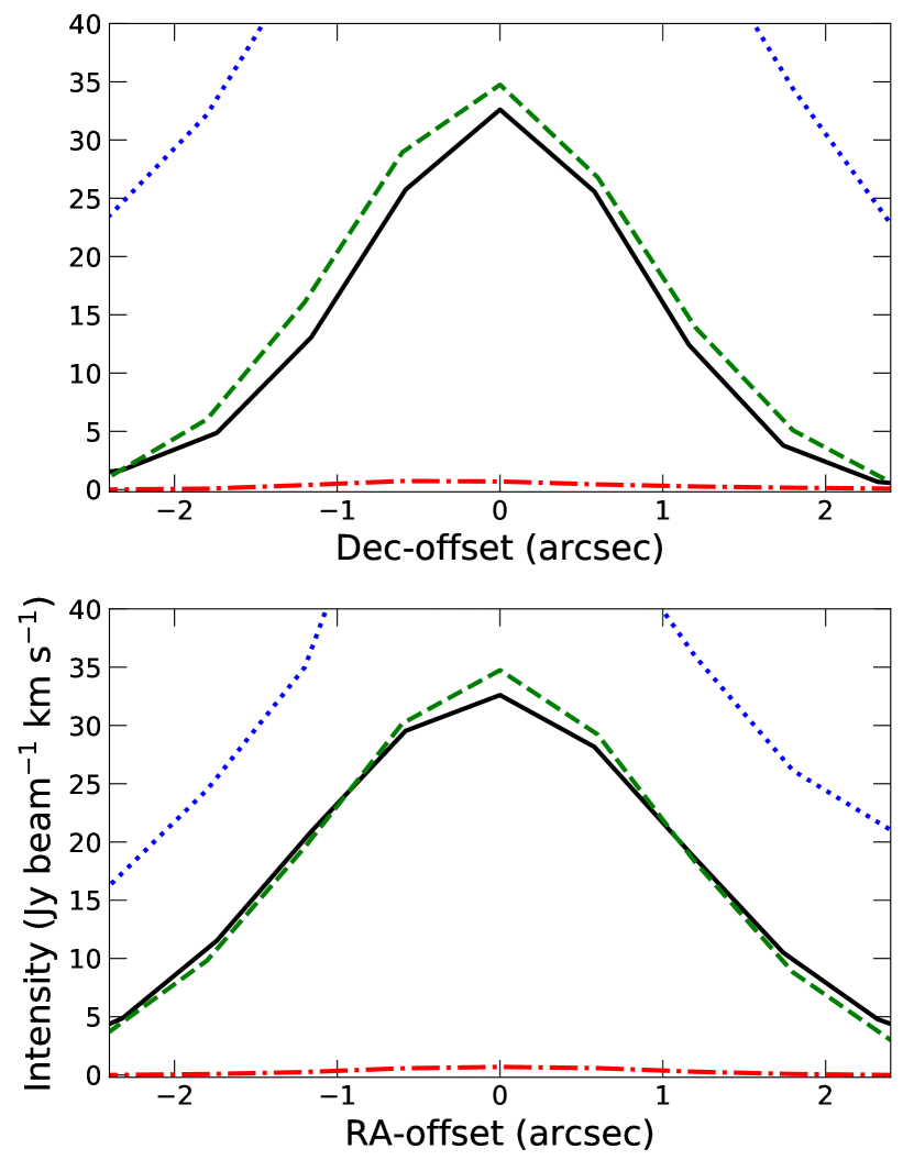
Figure 14: Observed (black line) and models zeroth moment map slices through the peak along the vertical (upper) and horizontal (lower) axes for $K=3$. The dashed green line corresponds to the best-fitting model with zero outflow reference velocity. The dotted red line corresponds to models with the same parameters as the best-fitting one but with the temperature step at $T_{0}=200$ K. The dash-dotted blue line shows a model with the same parameters as the best fitting model but with a constant abundance.

Fig. 15 shows the spectra at the peak of the zeroth moment map, which is equivalent to the spectra at zero offset in the pv maps, for each $K$ level. The best-fitting models do not match the width and the peak of the observed spectral line, mainly because the model infall and rotation velocities are high enough to produce double peaked spectra. Fig. 15 shows that models with lower stellar masses are needed to match them, but these models are not physically realistic given the stellar luminosity. In general, the abundance scales the line intensity. The best-fitting models prefer low abundances because larger values start to overestimate the values at the line wings. On the other hand, the observed lines are skewed towards higher velocities whilst the model lines are more symmetric.

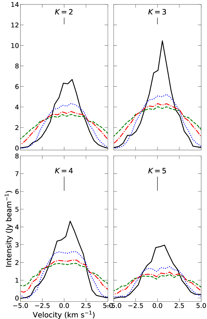
Figure 15: Observed (black line) and best-fitting model peak spectra (dashed green line) for (a) $K=2$, (b) $K=3$, (c) $K=4$ and (d) $K=5$. The dash-dotted red lines correspond to the best-fitting model with $M_{\star}=25$ M_☉. The dotted blue lines correspond to the best-fitting model with $M_{\star}=15$ M_☉.

The best-fitting models have a turbulent width of 2.0 km s^-1. Although this is in the upper end of our model grid, the lines are already wide due to the large rotation/infall velocities. The third model in the tally has a turbulent width of 1.5 km s^-1.

5 Discussion

5.1 70 µm morphology

Our detailed radiative transfer modelling has shown that the bipolar outflow cavities play an important role in reproducing the 70 µm observations. The modelling has allowed the fit of the extended emission at both this wavelength and the SED. The observed and model 70 µm images are elongated along the cavity axis. The results in Figs. 10 and 12 imply that the warm/hot dust in the envelope cavity walls bring an important contribution to the emission at 70 µm. Furthermore, the temperature distribution in Fig. 16 shows that cavity walls are being heated by the stellar radiation escaping through the outflow cavity more than other regions of the envelope. The figure also shows that the dust in the cavity is hotter than the walls, however there is less dust in the cavity. Hence the contribution of the envelope cavity wall is more important at 70 µm, which is also shown in the SED.

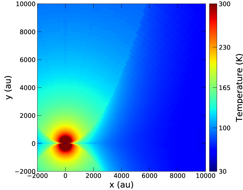
Figure 16: Temperature distribution in the mid-plane of the inner 10000 au region as obtained for the best-fitting model.

In the models of Zhang et al. (2013) the 70 µm emission is extended along the outflow direction. The origin of the extended emission in their models is due to dust in the outflow at distances larger than the core radius, otherwise the emission is dominated by the cavity walls of the envelope. They used a wide cavity angle (${\sim}100$°) thus at an inclination of 25° the observer is looking directly to the source, hence the emission of the cavity walls in their models is relatively symmetrical. In comparison, in our best-fitting model the line of sight passes through a section of the envelope.

5.2 Rotation of the envelope

Our analysis of methyl cyanide interferometric observations shows that they are tracing rotating gas at intermediate scales (${\sim}5000$ au) in the envelope of AFGL 2591. The velocities in the line of sight and the radiative transfer modelling imply that rotation dominates rather than infall or outflow motions. The direction of the rotation is consistent with the observations of smaller scales made by Wang et al. (2012). They also found that the linear velocity gradient in the HDO line pv map is 16.2 km s^-1 arcsec^-1 at a ${\rm PA}=0\degr$. Similarly, we calculated a linear velocity gradient from the pv maps at ${\rm PA}=6\degr$ for each $K$ line and obtained an average value of $13.3\pm 0.5$ km s^-1 arcsec^-1, which is consistent with slower rotation of the envelope in comparison to the disc. Thus the small-scale rotating motion observed in other molecules can be connected to the large scale motion traced by methyl cyanide.

We estimated a stellar mass of 35 M_☉ from the source luminosity. This mass is high enough for the models to produce double-peaked lines which do not fit the observations. The width of the line in these models are dominated by the large velocity gradient produced by a larger stellar mass rather than the non-thermal velocity width. We explored models with lower masses, and determined that for the Ulrich envelope with Keplerian disc model to fit the lines, stellar masses below 15 M_☉ are needed (see Fig. 15) which is unrealistic given the luminosity of the source (under this simple scenario where a single proto-star would form). Hence the rotation and/or infall motions of the inner envelope are slower than the ones predicted from the Ulrich envelope with a Keplerian disc. A binary or multiple system would provide less luminosity per total stellar mass, which would not fit SED. The slower rotation may be indicative of material being funneled through the envelope to the disc and/or the result of magnetic braking. Models at lower inclination angles (face-on), i.e. dominated by infalling motions rather than rotation, are discarded by the dust continuum models.

Benz et al. (2007) noted that their observations of HCN molecular line emission at the continuum peak were skewed towards the red as in the observations presented here for CH₃CN, whilst other lines (e.g. SO) were skewed towards blue. They interpreted the blue-skewed lines as produced by material in the inner region absorbing the red-shifted emission. Their observations however trace a smaller region close to the star, thus this can be explained by an optically thick disc. On the other hand, the CH₃CN radiative transfer modelling lines do not show any asymmetry close to the line centre. Although our radiative transfer modelling seems to favour models without outflows, this is not well constrained since the observations do not show a clear evidence of tracing outflow material. The width of the lines seems to be different in the outflow cavity than in the envelope. The wider lines are located in the outflow cavity and can be explained as turbulent motions of gas in the outflow. The emission from the region where the red-shifted outflow is located do not show the same trend. It can be argued that the emission is optically thick towards the red-shifted outflow, which is consistent with the inclination of the outflow axis with respect to the line of sight being closer to face-on.

5.3 Circumstellar matter distribution

The physical properties derived from our modelling are consistent with the current picture of AFGL 2591, but its density distribution is better constrained. Wang et al. (2012) estimated a disc dust mass between 1–3 M_☉ from the total flux at 1.4 mm from PdBI observations, and a disc radius of ${\sim}1300$ au (at 3.3 kpc) from a Gaussian fit to the 1.4 mm visibilities. We have shown that to fit the 1.3 mm extended configuration visibilities (Fig. 2b) a more massive and bigger disc is necessary. However, such a disc does not match the spatial extent of the 1.3 mm emission well (Fig. 3b). This can be explained by a closer to edge-on disc, which would look more compact in the outflow direction where the extent of the emission differ the most. Such a closer to edge-on disc can be the result of precession changing the PA and inclination angle at the smaller scales, but as argued in the previous section, the inner envelope favours an inclination closer to face-on. Johnston et al. (2013) obtained disc radii, which were also fixed to the centrifugal radius, of $3.5\times 10^{4}$ and $2.7\times 10^{3}$ au for their envelope with disc and control models, respectively. They also could not constrain the disc mass and radius as they did not fit the mm interferometric data.

The inclination with respect to the line of sight is consistent with the values in the literature (30–45°, e.g. Hasegawa & Mitchell, 1995; van der Tak et al., 2006) which are generally found based on geometrical considerations, and it is constrained between 25–35°. Larger values like those found by Johnston et al. (2013) are ruled out by the modelling since at 40° the red-shifted outflow cavity starts to emit in the near-IR. This discrepancy may be explained by the data and methods used. Although the red-shifted cavity is observed in the models at higher inclinations, the intensity is much lower than the peak of the blue-shifted cavity. Hence the red-shifted cavity emission will be negligible due to the lower surface brightness sensitivity of the 2MASS observations. Johnston et al. (2013) fitted the SED and 2MASS image profiles, thus their opening angle is not well constrained (cf. their fig. 4). Another reason the models rule out higher inclinations is that they require a larger envelope mass to compensate for the lower flux resulting from the higher inclination, and higher inclinations produce a deeper silicate feature which does not fit the mid-IR spectrum.

The inner radius is ${\sim}3$ times smaller than the one found by Preibisch et al. (2003) and Johnston et al. (2013). Although the sublimation radius was allowed to change in order to obtain a maximum dust temperature of 1600 K in the inner radius, the sublimation radii of the models did not increase noticeably. Smaller inner radii, near the sublimation radius, are also not strongly ruled out by Johnston et al. (2013). In order to analyse the effect of a larger inner radius on the near-IR observations, a modified version of the best-fitting model was calculated with an inner radius twice as large. This model did not improve the fit to the speckle visibilities ($\chi^{2}=49$). In addition, the fit to the $JHK$-bands observations is worse than the best-fitting model (reduced $\chi^{2}$ differences of about 46, 53 and 99, respectively).

Fig. 16 shows that the peak temperature at 1000 au scales reaches values between 200-300 K inside the outflow cavities, whilst in the denser cavity walls the peak temperature decreases to 200-250 K. Palau et al. (2014) obtained a temperature of 250 K at 1000 au scales from their simultaneous modelling of the SED for $\lambda>70\,\micron$ and SCUBA 450 µm and 850 µm radial profiles. Gieser et al. (2019) obtained a temperature distribution from 1-D LTE fitting of CH₃CN and H₂CO transitions of the combined NOEMA/CORE observations. From their equations, we obtain a value of ${\sim}220$ K at 1000 au from the 1-D LTE modelling. All these values are consistent with the temperature distribution from our dust emission modelling.

The parabolic shape of the cavity can help to explain the wider cavity opening angle close to the star as observed in maser emission (Sanna et al., 2012). The density in the cavity is also consistent with the one expected for an outflow (e.g. Matzner & McKee, 1999) and the opening angle is consistent with previous results (e.g. CS line modelling by van der Tak et al., 1999, maser emission from Sanna et al., 2012). Due to the lack of data, previous modelling of MYSOs used a constant small density (or empty) in the cavity (e.g. de Wit et al., 2010). This is not preferred in the modelling, as a constant density tends to produce more extended emission in the near-IR than observed. For a fixed cavity density distribution exponent, the density is determined mainly by the near-IR observations and the near/mid-IR regime of the SED. If the gas in the cavity is expanding isotropically, the outflow rate $\dot{M}_{\rm out}$ can be described as

$$\dot{M}_{\rm out}=4\pi r^{2}v_{\rm out}\rho_{\rm cav}\,,$$ (4)

with $v_{\rm out}$ the outflow velocity and $\rho_{\rm cav}$ the cavity mass density at radius $r$. The outflow rate is roughly 10 per cent the accretion rate $\dot{M}_{\rm acc}$ (e.g. Richer et al., 2000; Kölligan & Kuiper, 2018). If the accretion rate is $\dot{M}_{\rm acc}=\dot{M}_{\rm env}$, an outflow velocity $v_{\rm out}=260$ km s^-1 is obtained by solving eq. 4 with the values in Table 8. This velocity is within the range assumed by Preibisch et al. (2003) for the expansion of the loops (100–500 km s^-1) based on the ¹²CO line wings in the observations of van der Tak et al. (1999). For the radiative transfer model cavity density, the outflow velocity should be in the range 200–320 km s^-1 for infall rates within 20 per cent of the best-fitting model.

In general, the 450 µm and 850 µm images from the modelling are not elongated along the cavity axis. For the best-fitting model, the major-to-minor axis ratio of 2-D Gaussians fitted to the model images is ${\sim}1$ at both wavelengths, instead of ${\sim}1.3$ as observed (cf. Section 2.3.2). Elongation along the cavity axis was predicted by de Wit et al. (2010) for 350 µm observations of the MYSO W33A, but this is not observed in the modelling presented here at pc scales. However, their source has a larger inclination angle (60° for their best-fitting model) and their cavity has a constant density distribution of $\rho\approx 2\times 10^{-20}$ g cm^-3. Our results indicate that the elongation may be the result from earlier stages in the core formation and/or later evolution rather than produced by the cavities. To a lesser extent and as stated in Section 2.3.2, changes in the PSF may also help to explain why the models are not elongated.

Similarly to other molecules, the methyl cyanide abundance needed to be defined as a piecewise function in order to fit the extension of the emission and the ratios between different $K$ lines. Fig. 14 shows that a constant abundance model produces much more extended emission. Moving the temperature step from $T_{0}=100$ K to 200 K underestimates the peak zeroth moment, thus the $T=100-200$ K range is the most relevant one in order to fit the peak of the zeroth moment emission. The inclusion of a step at 230–300 K was not needed during the line radiative transfer modelling. This jump should increase the abundance of N-bearing molecules in the inner hotter regions (e.g. Rodgers & Charnley, 2001). Such temperatures are reached in regions much closer to the star which are not resolved by the methyl cyanide observations presented here. The gas temperature from the chemical modelling of the high-resolution NOEMA/CORE A+B+D data by Gieser et al. (2019) also does not go above ${\sim}220$ K at the peak of the emission. Further refining of the radiative transfer grid is also needed in order to further explore the changes in abundance.

5.4 Multi-wavelength modelling

Here we discuss several aspects of the modelling procedure. First we discuss the sensitivity of the model parameters to our observations and the selection of the best-fitting model given the large amount of data available for this work. Then we suggest improvements to the modelling with a focus in an observational aspect to constrain the less sensitive parameters and a theoretical aspect to improve the physical model, and thus obtain a better interpretation of the data for this and other MYSOs.

5.4.1 Sensitivity of model parameters

In total there are 15 free parameters defining each density distribution and heating source for model types A–C without including the dust models, the stellar mass and stellar radius. Additionally, there are 3 free parameters describing the kinematics of the gas. The inner radius depends on other parameters, and a few of them are not expected to be well-constrained by the modelling based on the observations available. These include the parameters defining the disc flaring and density structure (3 parameters), and the stellar temperature. The latter converged to different values for the three types of models presented in Johnston et al. (2013), but their inner radius, which was not well-constrained, was a multiple of the sublimation radius which in turn depends on the stellar temperature. Therefore, there are 10 free parameters which can be constrained by the continuum observations (see column “constrained by” in Table 8).

We calculated grids of models for parameters that can be well constrained by the observations available: inclination angle, cavity opening angle, envelope infall rate, disc mass and disc/centrifugal radius. These grids allow us to estimate the uncertainties of the varied parameters. Fig. 17 shows $\chi^{2}$ maps as a function of tentatively correlated parameters for specific observations.

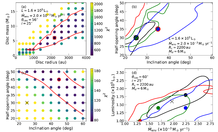
Figure 17: $\chi^{2}$ maps in parameter space. (a) $\chi^{2}$ of 1.3 mm extended configuration interferometric visibilities in the disc mass/radius plane. The red contour correspond to a 50$\sigma_{\chi^{2}}$ level with $\sigma_{\chi^{2}}=10$. The dot with red border marks the minimum value. (b) Minimum $\chi^{2}$ value (dots) and 5$\sigma_{\chi^{2}}$ (see online Table 13) contour level for the SED (black), and $J$ (red), $H$ (green) and $K$ (blue) observations in the cavity half-opening/inclination angle plane. (c) Herschel 70 µm $\chi^{2}$ map in the half-cavity opening/inclination angle plane. The dot with red border marks the minimum value and red contour corresponds to the 5$\sigma_{\chi^{2}}$ level with $\sigma_{\chi^{2}}=1$. (d) Same as (b) but for the luminosity/infall rate plane. The black cross marks the values adopted for the best-fitting model.

Fig. 17(a) shows the $\chi^{2}$ values for 1.3 mm extended configuration visibilities in a grid of models with varying disc mass and radius, and the other parameters equal to the best-fitting model ones. From the figure, we estimate an error of half the parameter resolution in this region of the grid, i.e. errors of 200 au in disc radius and 1 M_☉ in disc mass. We explored the correlation between these parameters and other observations, and found that in general IR observations (including 70 µm) and the SED prefer smaller disc radii. On the other hand, sub(mm) observations prefer models with bigger discs and higher masses. However none of these observations constrained these parameters as well as the 1.3 mm extended configuration visibilities.

The inclination angle and cavity opening angle plane in Fig. 17(b) shows that the minima of the SED and $H$-band observations coincide, whilst the $J$- and $K$-bands also coincide but at higher angles. However, the contour levels show that the latter have flatter $\chi^{2}$ distributions than the former, and Fig. 7 shows that good fits are obtained for the $J$- and $K$-bands at the best-fitting angles. The error in this case is dominated by the SED, because its $\chi^{2}$ distribution is more steeper than the other observations as pointed by its contour. We estimate an error of 5° for both angles. For models with constant envelope infall rates, the SED is best fitted by models with higher values for both angles as the luminosity increases. A similar behaviour is observed in the best fits of the $JHK$-bands, but due to the Monte Carlo noise the positions of the minima are more erratic. On the other hand, if the luminosity remains fixed the inclination angle of the best-fitting model to the SED decreases as the envelope infall rate increases, and there is not a clear trend in the values of the cavity opening angle. This is consistent with a deeper silicate feature at higher envelope infall rates (higher envelope masses) which is compensated by a lower inclination angle. The same is observed in the minima for the $JHK$-bands observations.

We did not use the 70 µm to constrain the inclination and cavity opening angles. The 70 µm distribution in Fig. 17(c) shows that this observation is fitted by larger values for both angles. This is probably pushed by the higher fluxes in the blue-shifted cavity as observed in the horizontal slice in Fig. 1. The inclination angle affects mainly the extension of the emission along the outflow cavity whilst the change in opening angle affects both directions but the change is more subtle. However, the increase in these angles does not increase the emission closer to the source as in the horizontal slice. In addition, the density distribution cannot account for e.g. inhomogeneities in the cavity, which may improve the fit. Submm observations are best fitted by models with lower opening angles, except for the 1.3 mm extended configuration visibilities which prefer slightly larger values. The latter are best fitted by slightly larger inclination angles (mainly in the 30–40° range) than the best-fitting model one. Even though we did not calculate a new grid of disc mass and radius with the best-fitting values for the inclination and cavity opening angles, Fig. 2 shows that a relatively good fit is obtained.

In Fig. 17(d) we show a cut in the stellar luminosity and envelope infall rate for the best-fitting inclination and cavity opening angles. In the figure, the position of the best-fitting model does not coincide with any of the individual observations, but it is in the intersection of the contours of the observations. Its position is at the same distance to the SED and the $H$- and $K$-band observations, hence it provides relatively good fits to them. The distribution of $\chi^{2}$ values for the $J$-band image is flatter than the other observations. From these grids, we estimate an error in the envelope infall rate of $0.2\times 10^{-3}\,\mbox{M${}_{\sun}$}\,{\rm yr}^{-1}$, i.e. roughly 10 per cent of the best-fitting model, and an error of $0.2\times 10^{5}$ L_☉ for the stellar luminosity. The minima for the best-fitted models to the 70 µm and 1.3 mm compact configuration data are generally located towards the higher end of luminosity and infall rate in the grid, whilst the $K$-band speckle and the SCUBA radial profiles prefer values in the lower end of the grid of these parameters. The minima of the 1.3 mm extended configuration prefer higher luminosities and lower infall rates than the best-fitting model.

Fig. 18 shows the position of the minima for grids with changing cavity opening angles and inclinations. For a fixed cavity opening angle (Fig. 18a), in the best-fitting models of the SED the luminosity increases and the infall rate decreases as the inclination angle increases. This is expected because as the inclination angle increases the silicate feature is increasingly deeper, whilst a larger opening angle overestimates the fluxes between ${\sim}2-8$ µm because this range is the most affected by the cavity emission (see Fig. 10). Hence, the envelope infall rate must decrease and the luminosity increase to compensate for the loss of flux in the envelope emission. On the other hand, in the best-fitting models of the $JHK$-band observations the luminosity and the infall rate decrease as the inclination increases. For a fixed inclination angle (Fig. 18b), in the best-fitting models of the SED and the $JHK$-band observations the infall rate increases as the opening angle increases, and in the case of the SED the luminosity slowly increases.

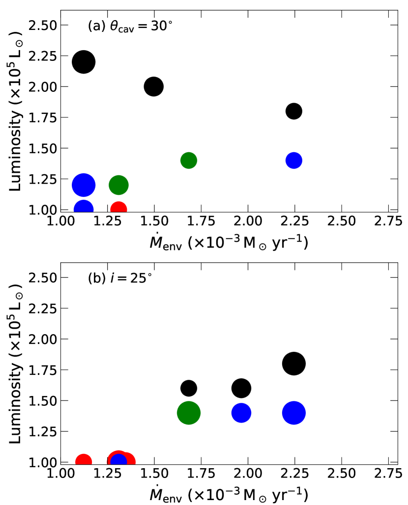
Figure 18: Position of the minimum $\chi^{2}$ in the luminosity-envelope infall rate plane for different (a) inclination angles and (b) cavity opening angles. The colour of the circles represent the SED (black), and $J$ (red), $H$ (green) and $K$ (blue) observations. The sizes of the circles increase with inclination angles (25, 35, 45°) and cavity opening angles (25, 28, 30°).

As part of the visual inspection step, we explored models with different cavity properties. Between models with cavity shape exponents $b_{\rm cav}=2$ and 1.5, the SED and the near-IR observations are best fitted by the former. Models with lower cavity shape exponents the minimum $\chi^{2}$ has a larger inclination angle by 5° between the shape exponents explored. For larger cavity shape exponents, the line of sight crosses a wider section of the envelope for a fixed inclination and cavity opening angle, hence the difference in minimum inclination angle. Models with a steeper density distribution tend to fit the SED best, reaching a factor of ${\sim}2$ difference between the $\chi^{2}$ of a constant and a $p_{\rm cav}=2$ density distribution. Similarly, the $J$- and $H$-band observations also favour steeper density distributions, whilst the $K$-band observation prefer intermediate exponents. None the less, the difference in $\chi^{2}$ is not as sharp as for the SED. A decrease in the cavity reference density of a factor of ${\sim}2$ or larger increases the $\chi^{2}$ of the SED by a similar factor, but the fit is less sensitive to changes of $0.2-0.4\times 10^{-21}$ g cm^-3. To fit the near-IR observations including the speckle interferometry, different combinations of the cavity parameters can produce noticeable changes as these determine the amount scattered emission. Some combinations produce local minima in $\chi^{2}$ values for the UKIRT observation fit, with comparable values between these minima. Given that the emission is not homogeneous, different values may be trying to fit different sections of the cavity. In general, cavity reference densities of 2 or more orders of magnitude smaller than the best fitting values for the SED are required to fit well the speckle visibilities, with increasingly larger density values for flatter density distributions. All in all, it cannot be ruled out that a different combination of the 5 parameters determining the aspect of the cavity may produce better results as these are probably degenerate, and we cannot break these degeneracies because the models cannot account for the inhomogeneities observed.

As expected, models with higher submm dust opacities, such as WD01, require a lower accretion rate, i.e. lower envelope mass, to match the submm points, but still within ${\sim}20$ per cent of the best-fitting model value. Another parameter that determines the envelope mass is its radius which is constrained mainly by the 850 µm intensity radial profile. Values between ${\sim}1.5-2.5\times 10^{5}$ au fit this profile at least up to 40 arcsec. The simulated observation did not take into consideration chopping during the real observations, which can make the observed radius smaller.

Although models with different flaring, scale heights and vertical density exponents were calculated (cf. online Appendix A.1.3), none of them improved the overall fit. Since most of the observations are not sensitive enough to these parameters, an accurate validity range cannot be given.

Stellar parameters are difficult to constrain since the proto-stellar emission cannot be observed directly in the near-IR. By taking into account the ratios of dust extinction/emission and scattering from our best-fitting model, we tried to constrain the stellar temperature by using the highest resolution near-IR point source data. However, the continuum is still dominated by photons scattered or emitted by dust, so this did not allow us to constrain the stellar temperature due to the low amount of direct stellar photons predicted by the model.

On the other hand, the line fitting is affected mainly by the abundance and line width for a fixed stellar mass. This was taken into account during the developing of the model grids. We estimate that the data can be sensitive to a finer grid of abundance values, with steps of e.g. $0.1\times 10^{-8}$. The line width can also be better explored by a finer grid, but with lines whose width is not dominated by the gas kinematics.

5.4.2 Best-fitting model selection

In our analysis we have used two methods to select the best-fitting models: one based on the ranking of $\chi^{2}$ values of each observation to select a seed model from the visual fit to dust continuum observations (Appendix A.1.2, online) and to select the line best-fitting model (Appendix A.3, online), and another method where we develop a grid of models to fit specific dust continuum observations and parameters (Appendix A.2, online). The former ranking method has been used by a few authors rather than using a e.g. $\chi^{2}$ goodness of fit statistic. Jørgensen et al. (2002), who combined SED and submm intensity profiles, argue that the $\chi^{2}$ values cannot be combined because the observations are not completely independent, thus it is not statistically correct to combine them. They also argue that intensity profiles and SEDs constrain different parameters of the density distribution. Williams et al. (2005) add that the $\chi^{2}$ values are in different numerical scales, thus they should be compared in an ordinal way. It can also be added that e.g. radial profiles can have a number of data points comparable to the SED, thus certain wavelengths will carry more weight in a total $\chi^{2}$. In order to explore this further, we show in Table 9 the continuum best-fitting models for the visual inspection step selected by using a total reduced $\chi^{2}$ and an average reduced $\chi^{2}$.

The best-fitting model as selected by the total reduced $\chi^{2}$ has a hotter star (36000 K) with the same luminosity, a larger envelope ($R_{\mathrm{out}}=270000$ au) and a slight higher accretion rate ($\dot{M}_{\mathrm{env}}=1.4\times 10^{-3}\,\mbox{M${}_{\sun}$}\,\mathrm{yr}^{-1}$) than the best-fitting model as selected by ranking during the visual inspection step. Their discs are the same except for the flaring and vertical density exponents, and their cavities have the same density distribution. As was shown in Section 4.1 and in Fig. 17 higher inclination and opening angles are preferred by the 70 µm observations but not by the $J$ and $H$-band ones, and the SED. It can also be seen in Table 9 that better $\chi^{2}$ values than in the best-fitting model by ranking are obtained in those observations with a higher number of points, namely the UKIRT $K$-band and 70 µm observations. Hence, this method for selecting the best-fitting model is dominated by the observations with a larger number of points.

The best-fitting model selected by the average $\chi^{2}$ is a type C model equal to the best-fitting type C model selected by ranking (see online Table 15), except for the envelope radius (200000 au). As argued, this type of models do not fit the near-IR observations and the SED. In general, this method gives more weight to observations which have in general a high $\chi^{2}$ value, namely the 1.3 mm NOEMA observations. It also reflects the difference in $\chi^{2}$ scale between the different observations. If all the observations were well fitted ($\chi^{2}\sim 1$) then this best-fitting model should be the same as the ranking one.

In general the method used in the visual inspection fitting is independent of the intrinsic $\chi^{2}$ scale of each observations and the number of points of each one. Overall the best-fitting model selected by ranking provides a good fit for key observations and its total and average $\chi^{2}$ values are relatively close to the best-fitting ones selected by these two $\chi^{2}$. The disadvantage of the ranking is that it reduces the difference between models with a large difference in $\chi^{2}$ or increases it for models with similar $\chi^{2}$.

On the other hand, in the grid modelling step of Fig. 11 (see also Appendix A.2, online) we determined the best-fitting model from the intersection of confidence regions in parameter space built from $\chi^{2}$ values for different dust continuum observations. This procedure is commonly used to constrain parameters in cosmological models. The advantage of this method is that it does not depend on the intrinsic scale of the $\chi^{2}$ values and does not reduce the differences in $\chi^{2}$ value between models. However, prior knowledge of the effect of each parameter in the fit to each observation is needed, and it requires more computing time to develop a grid. Hence combining this method with a prior filter from our visual inspection fitting improved the $\chi^{2}$ values of key observations.

5.4.3 Dust size distribution and grain growth

In order to explore the change in dust from within the envelope or disc, we derived spectral indices based on dust emission at different scales from single-dish and interferometric observations in the radio/submm regime. The former traces cold dust located in the large-scale envelope, whilst the latter trace scales of a few 1000 au. The dust optical depth is assumed to follow a power law $\tau\propto\nu^{\beta}$ in this regime (optically thin). If it is further assumed that the emission is in the Rayleigh-Jeans regime, the fluxes are then $F_{\nu}\propto\nu^{\beta+2}\propto\nu^{\alpha}$. Fig. 19 shows the observations made at different scales and the indices $\alpha$ of the power law fitted to the single dish, mm and radio interferometry data individually.

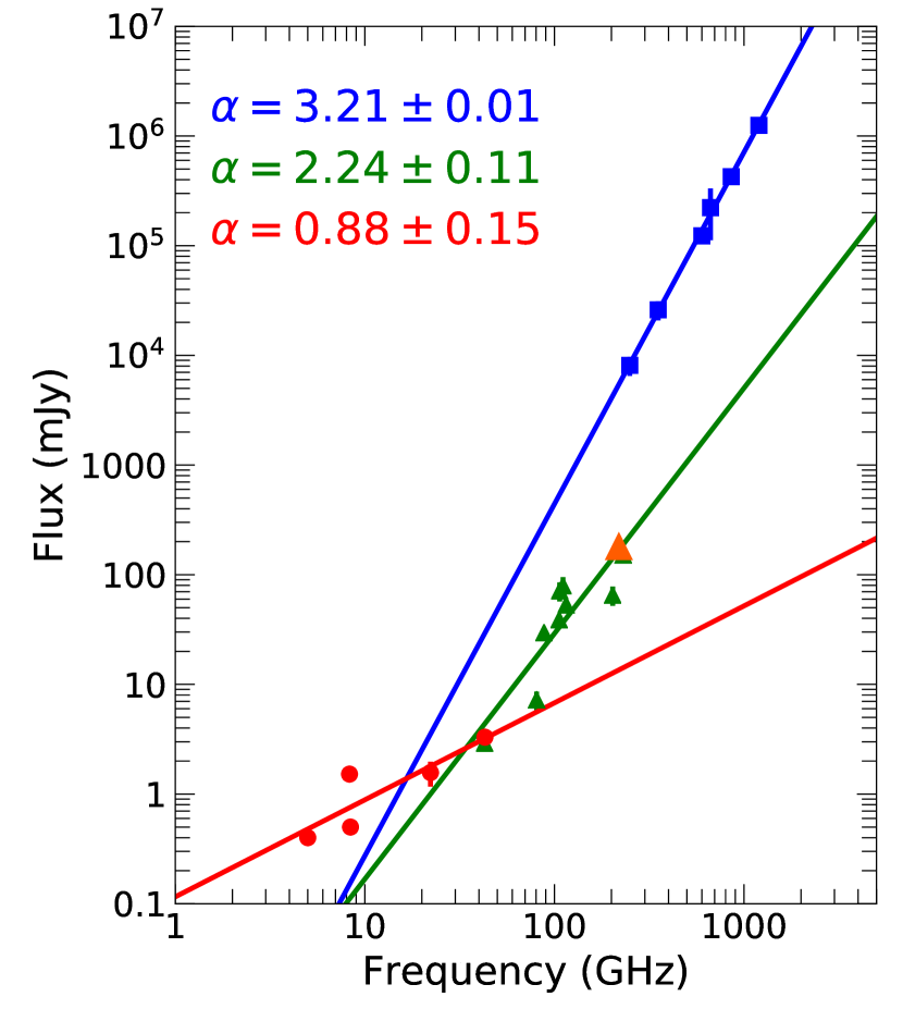
Figure 19: SED of the cm/submm regime as observed at different scales. Blue squares fluxes correspond to single-dish observations and are presented in Table 6. The orange triangle corresponds to the 1.3 mm extended configurations flux in Table 3, and the green triangles come from mm interferometric observations from van der Tak et al. (1999), Johnston et al. (2013) and Wang et al. (2012). Red circles are radio/mm interferometric observations from Campbell (1984), Tofani et al. (1995), Trinidad et al. (2003), van der Tak & Menten (2005) and Johnston et al. (2013). The slopes of the fitted lines are listed in the upper left corner. If the emission is from dust, the dust emissivity slope is $\beta=\alpha-2$.

Dust models with shallower emissivity indices (e.g. WD01, see online Table 12) fit the $\lambda>70$ µm regime of the SED better than dust with steeper spectral indices (e.g. KMH, OHM92), and allow the fit of visibilities at smaller baselines in the 1.3/1.4 mm with smaller discs that better reproduce the 1.4 mm emission. This is supported by the emissivity index derived from single dish observations ($\beta=1.2$ from Fig. 19). However, shallower emissivity index models, i.e. models with larger grains (cf. online Table 12), are not good at fitting the mid-IR regime and show an excess in emission along the cavity in the near-IR images because larger grains scatter more photons.

The dust emissivity index derived from interferometric observations is $\beta=0.2$. This shallower emissivity index implies that larger grains are responsible for the mm disc emission, thus it may be evidence of grain growth in the denser regions, i.e. the disc, of the MYSO. However, contamination from free-free emission can contribute to this index, hence a higher emissivity index cannot be ruled out. Although the best-fitting model from the visual inspection step favours a disc with smaller grains, good fits to the 1.3 mm extended configuration visibilities can be obtained with larger grains (W02-3 grains), albeit reducing the disc mass. On the whole, both types of grains actually do a good job at reproducing the observations, so there is not strong evidence that grain growth is needed to explain the data.

The spectral index of radio/mm observations and 3.6 cm observations (e.g. Trinidad et al., 2003; Johnston et al., 2013) points towards the presence of a jet or wind with $\alpha\sim 0.6$. Hence, the spectral index from mm interferometry may be steeper if the contribution of the jet/wind emission is subtracted, which will depend on the turnover frequency of the jet emission.

The presence of different dust properties to those used here is also supported by modelling of near-IR polarimetric observations of Simpson et al. (2013). They found that elongated dust grains rather than spherical ones can reproduce their observations better. Therefore, the dust properties may be different depending on the physical conditions at different positions, e.g. dust in the cavity walls is being shocked by the outflows or dust in colder regions may develop ice mantles. This may allow dust with $\beta=1.5$ to be present in colder regions of the envelope, thus improving the fit of the submm observations, and dust with $\beta=2.0$ to exist in hotter or shocked regions like the cavity walls, which may improve the mid-IR fit.

5.4.4 The Ulrich solution limitations

The Ulrich (1976) analytical solution for the accretion problem is able to reproduce some of the observed features. However, we could not find one model that can fit all the observations together. In particular, the results of the continuum and CH₃CN line modelling are contradictory. For instance, the stellar mass required by the Ulrich envelope with Keplerian disc velocity model is ${<}15$ M_☉which is much smaller than the one inferred from the source luminosity. This problem cannot be solved by changing the inclination angle, as lower inclination angles do not provide good fits to the $J$- and $K$-band observations. The slower observed rotation than the one suggested by the theoretical model may require the effects of magnetic braking to slow down the rotation of the disc and inner envelope. These limitations on the physics included in the Ulrich solution do not allow us to obtain better results.

Additionally, the simplicity of the models, where the clumpiness of the cavity or the presence of nearby sources are not taken into account, also limits the quality of the fit. The high-resolution 1.3 mm extended configuration observations in Fig. 3(b) recover more extended emission than the previous 1.4 mm observations from Wang et al. (2012), and show that the emission is more clumpy/less axisymmetric than the previous observations. This has also been observed in other MYSOs, e.g. high-resolution Atacama Large Millimeter/submillimeter Array (ALMA) observations of W33A (Maud et al., 2017). In the case of W33A filaments resembling spiral arms has been interpreted as accretion flows (Izquierdo et al., 2018). The velocity distribution in these accretion flows can be modelled with an Ulrich envelope by selecting some of its streamlines (e.g. Tobin et al., 2012, for low-mass star forming regions). Hence a full Ulrich envelope, rather than selecting some streamlines, is less likely.

Simulations with magnetic fields and radiation transfer show promising results. The radiation-magnetohydrodynamics (RMHD) simulations of early stages in the formation of high-mass stars calculated by Commerçon et al. (2011) show that magnetic fields and radiation can reduce the fragmentation during early stages in the formation of massive stars. The collapse of a $10^{3}$ M_☉ rotating molecular cloud investigated by Peters et al. (2011) through RMHD simulations also shows that magnetic fields can reduce fragmentation and that they are important in transporting angular momentum at local scales. Furthermore, the RMHD simulations of Myers et al. (2013), which explore a larger time evolution of a collapsing core with an initial power law density distribution index of –1.5, show that magnetic fields can remove angular momentum from the infalling material through magnetic braking whilst still forming a massive star (20 M_☉). Their models can still form an accretion disc but their centrifugal radii are ${<}50$ au, thus smaller than the one of AFGL 2591. Larger accretion discs can be obtained when non-ideal MHD effects are taken into account (Kölligan & Kuiper, 2018). These RMHD models also show that the matter is accreted into the disc from filaments which have collapsed within the envelope at scales of 5000 au in the mid-plane. However, these models do not include feedback from an outflow.

The non-magnetic simulations by Klassen et al. (2016) produce a Keplerian disc but they focus on 1000 au scales, thus in the transition from the envelope to disc. They also have a higher rotational to kinetic energy ratio than Myers et al. (2013) by a factor of ${\sim}5-30$, and impose an initial solid body rotation. In the 3-D radiation-hydrodynamic simulations of Meyer et al. (2018), Keplerian discs are produced which develop spiral arms and fragment into a multiple stellar system. The 2-D simulations of Kuiper et al. (2015, 2016); Kuiper & Hosokawa (2018) show the effect of radiation on the outflow cavity and its widening from an initially slowly rotating core. The cavity distributions in these models resemble the near-IR observations of AFGL 2591. However, they do not include magnetic fields. Newer simulations are including the effects of an increasing number of physical processes, e.g. in the Kuiper & Hosokawa (2018) simulations the effects of photo-ionisation from a potential Hii region are included. These and future simulations have the potential to describe better the physical properties in MYSOs from high-resolution observations.

5.4.5 A recipe for future multi-wavelength modelling

The diagram in Fig. 20 summarises the steps necessary for modelling multi-wavelength data with 2-D radiative transfer models in order to obtain better constraints to the model physical parameters from specific observations. The modelling is performed in three steps with increasing refinement of key parameters at each step and complexity in the modelling, and each step is divided in a series of sub-steps. The sub-steps are in sequential order, although some of them can be swapped or skipped depending on the available data. Here we discuss the main features and caveats of each step.

Figure 20: Steps for modelling and bringing up constraints from MYSOs observations. Parameters under “cavity shape” are opening angle and cavity shape exponent. Parameters for “disc shape” are scale height and flaring exponent. The item “outflows” refers to molecular line observations of outflows. Simple modelling includes fitting with templates or with models such as 2-D Gaussians.

The aim of the first step is to obtain initial values and constraints for the 2-D model parameters in Table 8. The observations for each parameter in Fig. 20 are in order of preference. Some of these parameters will then be further constrained in the next steps. The initial value for the luminosity can be obtained from model templates (e.g. Mottram et al., 2011a). These model templates can account for rotationally flattened envelopes and cavities (e.g. Robitaille, 2017), hence obtaining an initial range of inclination angles and cavity properties can help to constrain the templates. We have listed the disc shape (disc flaring exponent, scale height) in two sub-steps. The first one is for cases of discs closer to edge-on using imaging whilst the second relies on the modelling of mid-IR visibilities (e.g. di Folco et al., 2009). Although measuring these disc properties, and to a lesser extent the disc radius, from mid-IR observations is desirable as they are tracing optically thick emission from the surface of the disc, some MYSOs may still only be partially resolved in the mid-IR in high-resolution observations (e.g. de Wit et al., 2009). Envelope and disc masses measured from dust emission are obtained by estimating a dust temperature from the SED. These are a good approximation in terms of order of magnitude for the next step. Some deeply embedded MYSOs may be weak in the near-IR, hence to derive the properties of the outflow cavity shape (inclination angle, opening angle, shape exponent) molecular line emission tracing the outflow (e.g. CO) can be used instead. However, precession of the outflow axis can affect the determination of the cavity geometry, PA and inclination angle. In such cases, high-resolution mm interferometric observations tracing the disc can provide further constraints. In general, most geometric properties are degenerate due to projection effects, except at extreme inclination angles.

In Step 2, we have integrated the main relations found in our modelling and added further steps to constrain other parameters. All the sub-steps in this step constrain the physical parameters through 2-D axisymmetric modelling and are relatively independent from each other. Some sub-steps iterate between parameter-observations relations in order to optimise the modelling, however $n$-dimensional optimisation, with $n$ being the number of parameters in the sub-step, can also be performed. Additional parameters constraining the velocity distribution are introduced in this step after modelling the continuum data. Initial values for these parameters can be derived from the luminosity (stellar mass) or analysis of the spectra (outflows).

The objective of the final step is to model 2-D axisymmetric features of specific observations in order to shrink the area in $\chi^{2}$ space in the relations of the previous step. Hence the sub-steps in the previous step must be repeated with the new model and an additional iteration must be performed to constrain the parameters of the newly introduced features (see example in Fig. 20). Since the sub-steps are relatively independent, the introduction of other 2-D structures may not affect all the relations. For instance, introducing entrainment features to better model near-IR observations will likely not affect the envelope radius and disc properties. On the other hand, introducing a torus to explain mid-IR features (e.g. de Wit et al., 2011) can affect the disc properties as well as the envelope mass. Determining the orientation of the 2-D features should be straight forward because the orientation angles (PA and inclination) were constrained in the previous steps. This step requires that the comparison between model and observations is performed on a pixel-by-pixel basis for images in order to increase the number of data points needed to fit the increasing number of parameters in the model. Some of the additional model features may be geometrical rather than physical, hence this step may only constrain the physical parameters in the previous one. Non-axisymmetric features can then be introduced to the models to optimise the relationships in Step 2 (see Section 5.4.4 for examples).

6 Conclusions

We used spatially resolved dust continuum images between 1 to 1400 µm and the SED to study the dust density and temperature distributions, and methyl cyanide interferometric observations to study the inner envelope velocity distribution of the proto-typical MYSO AFGL 2591. We performed a multi-step radiative transfer modelling to constrain the physical model parameters and determined correlations between specific observations and model parameters. We show for the first time that the Herschel 70 µm emission is extended in the outflow direction and explain its extended nature as the result of dust emission from the outflow cavity, whose walls are heated by the radiation escaping through the less dense cavity medium. We found that the inner envelope is rotating and this rotation is slower than the disc.

We have attempted to fit a large number of observations with a unified physical model. The best-fitting model consists of an Ulrich envelope, a flared disc and bipolar outflow cavities with properties consistent with previous results. The presence of a disc is needed in order to fit NOEMA 1.3 mm extended configuration visibilities. We derive a disc mass of $6$ M_☉ and 2200 au radius. These values are relatively independent of the parameters determining the envelope/outflow cavities density distribution. The 450 µm and $K$-band speckle interferometry observations were not fitted well by the models.

This model cannot explain the observed CH₃CN pv maps, because the model lines are wider due to the high velocity gradients of the Ulrich envelope with Keplerian disc model. In addition, the model lines are not skewed like the observed ones. Accretion flows and magnetic braking may be able to explain why the inner envelope rotation is slower than predicted by the Ulrich envelope.

The physical limitations of the Ulrich solution, together with the simplicity of the models, do not allow an improvement over what we have done in this paper. 3-D self-consistent theoretical models should be tested in order to improve the fit to the observations. Additional improvement to the modelling and high-resolution multi-wavelength observations may also be needed to constrain these parameters. Future papers including higher-resolution data from CORE and other surveys will allow a more complete study of MYSOs to test these models.

Data Availability

The data underlying this article will be shared on reasonable request to the corresponding author. Parts of these data were derived from: WFCAM Science Archive (http://wsa.roe.ac.uk/), Herschel Science Archive (http://archives.esac.esa.int/hsa/whsa/), SCUBA Legacy Catalogues (http://www.cadc-ccda.hia-iha.nrc-cnrc.gc.ca/community/scubalegacy/). The $K$-band speckle interferometric data were provided by T. Preibisch by permission.

Appendix A Modelling details

The following sections describe in detail the modelling steps summarised in Fig. 11.

A.1 Dust continuum: visual inspection

In order to obtain the dust density and temperature distributions, we used the 3-D Monte Carlo radiative transfer code hyperion (Robitaille, 2011) to calculate SEDs and images produced by a dust distribution heated by a given heating source. We first performed a fitting by varying the model parameters based on $\chi^{2}$ values and visual inspection. In this step we explored different density distributions and dust models. This allowed us to constrain the range of values for some parameters and to identify correlations between parameters and observations. We then built model grids to constrain parameters strongly related to some of the observations, and to provide fitting uncertainties.

A.1.1 Density distributions

Table 10 presents the different density distribution types considered here, and further details can be found in Appendix B.1. For type A, we follow the nomenclature and fiducial values in Johnston et al. (2013, see also Table 11) in order to compare the results with their results. Types B and C are used to study the effects of different types of envelope and disc distributions on the fit. All these density distributions have been used and/or proposed to explain the emission of MYSOs.

Table 10: Density distributions.

Type	Density structuresa	$N_{\rm model}^{\mathrm{b}}$
A	Ulrich envelopec + flared disc	444
B	Ulrich envelopec + alpha disc	131
C	Power law enveloped + flared disc	52

^a All models include bipolar cavities.

^b Total number of models for each type.

^c Ulrich (1976).

^d $n\propto r^{-p}$ with $n$ the density and $r$ the distance to the source.

For the density distributions, we used the built-in hyperion functions. The values of the distributions were calculated at each cell of a spherical coordinate grid. The densities of all the components are defined between the inner and outer radii, and are defined to model a single source (AFGL 2591 VLA 3). We fixed the maximum radius of the grid to $3\times 10^{5}$ au, i.e. larger than the envelope radius. The optimal inner radius of the grid was chosen by hyperion based on the inner radius of the density distributions (the dust sublimation radius). To calculate the total density distribution, hyperion calculates the density distribution of each component in all cells. Then it replaces the cells within the bipolar outflow cavities, which were initially set to the envelope density, by the density of the cavity component, and finally it sums this with the disc component. The model grid had 700 cells with a logarithmic distribution in the radial direction and 200 cells with a sinusoidal distribution in the elevation direction ($\theta$ in spherical coordinates), thus improving the number of cells close to the inner radius and the mid-plane. For most of the models $5\times 10^{6}$ photons were used for the calculations (specific energy and imaging) in order to optimise the computing time, and we set the convergence criteria to that in (Robitaille, 2011).

A.1.2 Fitting procedure

Table 5 lists the data product type (image, intensity radial profile, visibility profile) that we used to compare the observations and the respective synthetic observation in order to extract spatial information. To obtain each of these data products from the code results and compare them with the observed ones, we binned the images to match the observed pixel size, rotated them to match the cavity position angle (259°; Preibisch et al., 2003) and convolved them with the respective PSF. The details about the processing of the model images can be found in Appendix C.

In order to determine a set of models that best fit our data, we first calculated the reduced $\chi^{2}$, for each of the datasets listed in Table 5 and the SED. The reduced $\chi^{2}$ were calculated after masking the non-relevant data (see Appendix C). Similarly to Williams et al. (2005), the rank of the models for each of these reduced $\chi^{2}$ was calculated, i.e. the rank of the models for each of the types of data. Finally, we combined these ranks to obtain an average rank per model. In the particular case of the $K$-band and 1.3 mm observations, where we have two measurements for the same wavelength, the average rank of the two observations was calculated at each wavelength before they were combined with the results from the other observations. As reference, the best-fitting model from this step is that with the lowest ranking.

A.1.3 Assumed parameters

Most initial parameters were taken from the results of Johnston et al. (2013), where we used average values of their two envelope with disc models, e.g. the disc scale height and density in the cavity. We also used initial parameters from de Wit et al. (2010) for the MYSO W33A, such as the envelope infall rate. The cavity density distribution ($\rho\propto r^{-p_{\rm cav}}$) and shape parameters ($z\propto R^{b_{\rm cav}}$) were taken from observations and theoretical models of outflows (e.g. Preibisch et al., 2003; Bruderer et al., 2010). These parameters were varied and new models computed based on the fitting statistics described in Section A.1.2 and a visual inspection of the results. Since analyses of the effects of changing each parameter in the model images and SED already exist (e.g. Alvarez et al., 2004), we built our models in this step from this knowledge and the previous studies of this source.

Table 11 summarises the input parameters and the ranges used for the models. Models with an envelope and a cavity were used to determine the stellar luminosity that best fits the SED peak and shape. We obtained a value of $L=1.6\times 10^{5}$ L_☉, which is slightly lower than the value in the literature ($L=2\times 10^{5}$ L_☉; Lumsden et al., 2013). The luminosity was fixed to this value for most models, but we also calculated models with other luminosities in order to improve some fits, e.g. $L=1.4\times 10^{5}$ L_☉ for models with WD01 dust (see below). The stellar spectrum was assumed to be that of a black body and its radius was calculated self-consistently with the temperature and luminosity. Since all the emission is reprocessed by dust and our observations are insensitive to the stellar temperature, we do not expect a large change in our results if a stellar atmosphere model is used instead.

Table 11: Parameter ranges used in the visual inspection and grid fitting steps.

Parameter	Visual	Grid
		Step 1	Step 2
Type A
Inclination angle ($i$)	20–40°(5°)	20–40°(5°)	20–60°a (5°)
Stellar temperature ($T_{\star}$/K)	10000–40000	18000
Stellar luminosity ($L_{\star}/10^{5}$ L☉)	1.4–2.0	1.6–2.0 (0.2)	1–2.6 (0.2)
Outer radius ($R_{\mathrm{out}}$/au)	100000–300000b	195000
Envelope infall rate ($\dot{M}_{\mathrm{env}}/10^{-3}\,\mbox{M${}_{\sun}$}\,{\rm yr}^{-1}$)	0.2–3.0	1.3–2.6	0.9–1.7 (0.2),
			2.0, 2.2–3.0 (0.4)
Envelope dustc	OHM92, KMH, WD01	OHM92
Centrifugal radius ($R_{\mathrm{c}}$/au)	100–1000	200–1000 (200),	2200
		1000–3800 (400)
Disc mass ($M_{\mathrm{d}}$/M☉)	0.25–4	0.5, 1, 2–18 (2)	6
Disc scale height at $r=100$ au ($h_{0}$/au)	0.1–11.0	0.6
Disc flaring exponent ($\alpha$)	2.25, 1.88, 2.5	2.25
Disc vertical density exponent ($\beta$)	1.25, 1.13, 1.5	1.25
Disc dustc	OHM92, W02-3	OHM92
Cavity half opening angled ($\theta_{\rm cav}$)	25–40°	28°	15–50° (5°)
Cavity shape exponent ($b_{\mathrm{cav}}$)	1.5, 2.0	2.0
Cavity density exponent ($p_{\rm cav}$)	0, 1.5, 2.0	2.0
Cavity reference densityd ($\rho_{\rm cav}/10^{-21}$ g cm-3)	$2\times 10^{-6}$–21	1.4
Cavity dustc	OHM92, KMH	KMH
Type B
Stellar Mass ($M_{\star}/\mbox{M${}_{\sun}$}$)	40	–	–
Disc accretion rate ($\dot{M}_{\mathrm{acc}}/\mbox{M${}_{\sun}$}\,{\rm yr}^{-1}$)	$1\times 10^{-4}$	–	–
Type C
Envelope power law index ($p$)	2.0	–	–
Envelope mass ($M_{\mathrm{env}}/10^{3}\,\mbox{M${}_{\sun}$}$)	1–5	–	–

Notes. Step 1 refers to the fitting of the 1.3 mm extended configuration visibilities to constrain the disc mass and radius. Step 2 was developed to constrain the envelope infall rate, luminosity, inclination and cavity opening angles (see Section A.2). The numbers in brackets indicate the spacing of the values in the grid.

^a The range depends on the opening angle for grids of luminosity and envelope infall rate, but all cover the 30–40° range.

^b As an exception, one model with radius 790000 au was calculated.

^c See Table 12.

^d Defined at a height $z=10^{4}$ au.

Based on Davies et al. (2011) calculations, we estimated a ZAMS stellar mass between $M_{\star}=30-40$ M_☉ for a stellar luminosity of $L=1.6\times 10^{5}$ L_☉. From eq. 6, the stellar mass and the infall rate are degenerate parameters for a given envelope density. The stellar mass is considered as a free parameter only in models with an alpha disc (type B models) as it determines the accretion luminosity ($L_{\mathrm{acc}}\propto M_{\star}$). The stellar mass can only be constrained by studying the molecular line emission. Since we perform the line modelling after the continuum fit, we can scale the envelope infall rate to match the envelope mass if needed.

The initial inner radius of the model, $R_{\rm in}$, was calculated using eq. 9 with a sublimation temperature of 1500 K. Sublimation of dust was allowed during hyperion iterations by decreasing the dust density in those cells exceeding an upper limit dust sublimation temperature of 1600 K. Although this temperature is higher than the one used to estimate the inner radius using the Whitney et al. (2004) method, the range of sublimation radius values are in a similar range (30–40 au). This upper temperature limit was reached by most models in each density component.

In this step, we kept the disc mass $M_{\mathrm{disc}}\lesssim 0.1\,M_{\star}$ and its radius below 1000 au, which are close to the values found by Wang et al. (2012), determined from the total flux of their interferometric observations at 1.4 mm. We explored more massive and larger discs during the grid fitting step (see Section A.2). For most models, parameters describing the disc flaring and vertical density distribution were fixed to the values in Johnston et al. (2013, $\alpha=2.25$ and $\beta=1.25$), and the disc radius was fixed to the centrifugal radius in most cases. In the few cases where we varied these parameters, their lower limits were those of a steady Keplerian disc in Alvarez et al. (2004, $\alpha=1.88$ and $\beta=1.13$), and upper limits of $\alpha=2.5$ and $\beta=1.5$. The scale height was chosen to produce a physically thin disc.

For type B models, the $\alpha$-disc parameters were fixed to their flared disc equivalent in type A models, whilst the envelope and cavity parameters were constrained in the same ranges as type A models. We expect the accretion rate to be a fraction of the infall rate. de Wit et al. (2010) found that the accretion rate can be three orders of magnitude smaller than the envelope infall rate for a compact (500 au) and less massive (0.01 M_☉) $\alpha$-disc to fit mid-IR observations of the MYSO W33A. From eq. (15) of Hosokawa et al. (2010), accretion rates slightly higher than $10^{-3}$ M_☉ yr^-1, which is comparable with the envelope infall rate, are expected at later phases when the star is settling into the main sequence. Since we do not have any observation to constrain this parameter (e.g. de Wit et al., 2010) and assuming that our source is relatively young (e.g. in the swelling phase of Hosokawa et al., 2010, which is consistent with the definition of MYSO), the disc accretion rate, which determines the accretion luminosity, was set to $1\times 10^{-4}$ M_☉ yr^-1 in most models, which is ${\sim}10$ per cent of the envelope infall rate in the models. For a typical disc with an inner radius of 35 au, outer radius of 100 au and 1 M_☉, an accretion luminosity of ${\sim}15$ L_☉ is obtained from eq. (6) of Whitney et al. (2003). Therefore, the main difference with the flared disc model is the density distribution. The Disc and cavity parameters in type C models were constrained in the same ranges as type A models.

The observed SED has 41 data points. In the images, the number of independent data points can be approximated as the area of the pixels within each observation mask divided by the solid angle of the PSF. If the PSF is assumed Gaussian then the solid angle is $\Omega_{\rm PSF}=2\pi\sigma_{\rm PSF}^{2}$ with $\sigma_{\rm PSF}$ the standard deviation of the PSF. This gives roughly 160 independent points for the 70 µm observation and 2700 for each UKIRT masked observation. For the other observations the number of fitted points ranges between 7–24, but the number of independent points should be around half of those due to the effect of the beam/PSF convolution. Therefore, the number of independent points, and considering that the observations trace different emitting regions, should be enough to constrain the effective 10 free parameters assuming that the data are good probes of these properties.

A.1.4 Dust models

A number of dust models with different optical properties were used during the modelling. The purpose of using different dust libraries is two-fold. On the one hand, changing the dust properties can improve the fit. On the other hand, they can provide information about the dust properties of each density component (e.g. disc, envelope). Table 12 lists the dust models used for each density component.

For the WD01 dust model, we calculated the dust properties using Mie theory together with the dust size distribution as calculated by the available online scripts and the dust dielectric functions of Laor & Draine (1993), so the dust properties are close to those published by Weingartner & Draine (2001). This dust model was recalculated in order to convert to the appropriate format for hyperion. The dust optical properties of OHM92 dust were imported from the dust files developed by de Wit et al. (2010) for the ho-chunk (Whitney et al., 2013) radiative transfer code, whilst the properties for W02-3 dust were imported from the same code library. The properties of the KMH dust model are readily available in hyperion.

We also used other dust libraries with different far-IR slopes for a few models (e.g. KMH dust with ice mantles), but we did not persist with them as they did not improve the fit. We did not include models 1 and 2 from Wood et al. (2002) in order to reduce the parameters in the fit, and we only use model 3 in order to analyse the effect of grain growth and because it is the dust model with the flattest emissivity index.

Table 12: Dust libraries.

Dust	Structures	$\beta^{\mathrm{a}}$	$a_{\rm min}$	$a_{\rm max}$	Size dist.	Ref.
			(µm)	(µm)
OHM92	envelope, disc, cavity	2.0	0.005	0.25	MRN+CDE	(1)
KMH	envelope, cavity	2.0	0.0025	–	MEM	(2)
WD01	envelope	1.7	0.00035	${\sim}1$	pl + log-normal	(3)
W02-3	disc	0.4	–	1000	pl	(4)

Notes. MRN is a power law with index –3.5, CDE stands for continuous distribution of ellipsoids, MEM corresponds to maximum entropy method fitted to data and which can be approximated by a power law plus an exponential, and pl stands for power law.

^a Dust emissivity index measured between $100-1000$ µm.

References. (1) Ossenkopf et al. (1992) silicates and MRN amorphous carbon grains (Mathis et al., 1977), see also de Wit et al. (2010); (2) Kim et al. (1994); (3) Weingartner & Draine (2001) for $R_{V}=5.5$; (4) Wood et al. (2002) model 3.

A.2 Dust continuum: grid fitting

To save computing power whilst concentrating on the constrainable parameters, we avoided running a grid consisting of 15 dimensions, and instead we used the parameters of a set of best-fitting models from the visual inspection step to build model grids for combinations of a limited number of parameters in order to fit specific observations. In this step we only varied the disc radius and mass, the luminosity, the envelope infall rate (i.e. the envelope mass), the cavity opening and inclination angles, in order to further constrain them. We did not limit the range of the parameters as strongly as in the visual inspection step. To process the models and the simulated observations we followed the same steps as in the previous section.

We divided the fitting procedure in two steps. In the first step we constrained the disc mass and radius from the 1.3 mm extended configuration visibilities by minimising the $\chi^{2}$ value. We then used the SED and UKIRT images to constrain the luminosity, envelope infall rate, and the inclination and cavity opening angles. A summary of the parameter space explored during each of these two steps can be found in Table 11.

To obtain a seed model, we determined the most common physical properties of the models in the visual inspection step with a total ranking equal to the best-fitting model ranking plus 100, which gave us a total of 15 different models. The properties of the seed model determined from these 15 models are listed in Table 11, these are fixed during all the fitting steps described below. All these 15 models are type A models (Ulrich envelope and flared disc). Since the stellar luminosity is less constrained by our observations, we inherit the stellar temperature from the control model in Johnston et al. (2013, 18000 K). We set the disc and envelope dust to the OHM92 model, however good fits may also be obtained with a disc with the W02-3 dust model by scaling the disc mass (disc masses with W02-3 are roughly less than half those with OHM92 dust).

In the visual inspection fitting we found a strong relation between the disc mass and radius with the 1.3 mm extended configuration visibilities. The parameters varied during this step are listed under Step 1 in Table 11. We did not develop a rectangular grid (evaluating all the combinations of disc mass and radius) in parameter space, but rather focus on a region which minimises the $\chi^{2}$ values. This region is closely related to the surface density $\Sigma\propto M_{d}R_{c}^{-2}$. Models with different inclination angles, envelope infall rates and luminosities were used to analyze their influence on the fit of the disc parameters. We determined the best-fitting disc radius and mass from the model with minimum $\chi^{2}$. The fit to the 1.3 mm visibilities was relatively independent on the luminosity, envelope infall rate and inclination angle, hence the disc properties were fixed during the following steps.

Then, we constrained the stellar luminosity, envelope infall rate, inclination and cavity opening angles. The stellar luminosity and envelope mass are strongly determined by the SED and to a lesser extent by the UKIRT observations, whilst the inclination and cavity opening angles can be fitted from the SED and UKIRT observations. We iterated between grids of luminosity and envelope infall rate at different inclination and fixed cavity opening angles, and grids of inclination and cavity opening angles at fixed luminosity and envelope infall values. The grids of luminosity and envelope infall rate were calculated at 5 inclination angles. We observed that the minimum $\chi^{2}$ for the SED requires larger inclination angles as the opening angles increases, hence the 5 values of the inclination angle varied depending on the opening angle but most models covered the 30–40° range in steps of 5°. From an initial grid at a seed cavity half opening angle of 28°, we used luminosity and envelope infall rate values at the minimum $\chi^{2}$ for the SED to compute a grid of inclination and cavity opening angles (see Table 11). We then repeated the procedure for a different cavity opening angle. In total we calculated grids of luminosity and envelope infall rate at 5 cavity opening angles (25, 28, 30, 35, 40°), and grids of inclination and cavity opening angles at 9 combinations of luminosity (1.6, 1.8, 2.0$\times 10^{5}\,\mbox{L${}_{\sun}$}$) and envelope infall rate ($1.1,1.3,1.5,1.7,2.0,2.2\times 10^{-3}$ M_☉ yr^-1). Thus, some regions of the parameter space were covered twice.

We could not find a region in the parameter space that minimised the $\chi^{2}$ values for the SED and UKIRT observations simultaneously. Moreover, we found that due to the probabilistic nature of the radiative transfer code, the values of the $\chi^{2}$ may vary for different runs of the same model. Hence, we can only give a region of the parameter space where the global minimum may be located. In Table 13 we list the values of the standard deviation of the $\chi^{2}$ values for 5 runs of a random model at different inclination angles. Since these values may depend on model parameters, we determined a conservative overall $\chi^{2}$ standard deviation in order to define a confidence region in the parameter space where the minimum may be located. The parameters of the best-fitting model were selected from a model at the intersection of the confidence regions of the observations. In the inclination and cavity opening angle plane, the best-fitting model is located at position of the minimum $\chi^{2}$ for the SED and $H$-band observation. The location of the best-fitting model in the same plane is shifted towards lower values with respect to the location of the minimum $\chi^{2}$ of the $J$ and $K$-bands. The position of the best-fitting model in the luminosity and envelope infall rate plane does not coincide with the location of the minimum $\chi^{2}$ of the observations, but it is located in a compact region of the parameter space with a relatively constant distance to the minimum $\chi^{2}$ positions for the SED, $H$- and $K$-band observations.

Table 13: Standard deviation of $\chi^{2}$ values from a random model run 5 times.

Observation	Inclination angle			$\sigma_{\chi^{2}}$
	$\sigma_{30\degr}$	$\sigma_{35\degr}$	$\sigma_{40\degr}$
SED	0.37	0.20	0.16	0.5
UKIRT $J$	2.4	2.6	2.1	3.0
UKIRT $H$	4.5	2.7	1.3	5.0
UKIRT $K$	19	20	18	20
NOEMA 1.3 mm ext.	5.1	5.8	7.4	10
Herschel 70 µm	0.5	0.6	0.7	1.0

A.3 CH₃CN molecular line modelling

Models for the $K=2-5$ lines were calculated using the line radiative transfer code mollie (Keto & Rybicki, 2010). We excluded the blended $K=0$ and 1 transitions (see Fig. 21) to ease the modelling/analysis and because these should not add any additional information. The code requires grids describing the density, temperature and velocity distributions of the gas, the abundance of the molecule with respect to the gas density and the width of the line. mollie calculates the molecular line emission at different velocities, i.e. it produces a data cube, under the LTE approximation for CH₃CN. Since the radiation field (the gas temperature) is calculated from the continuum modelling and the LTE approximation is used, mollie uses the input distributions to calculate the level populations and produce the images.

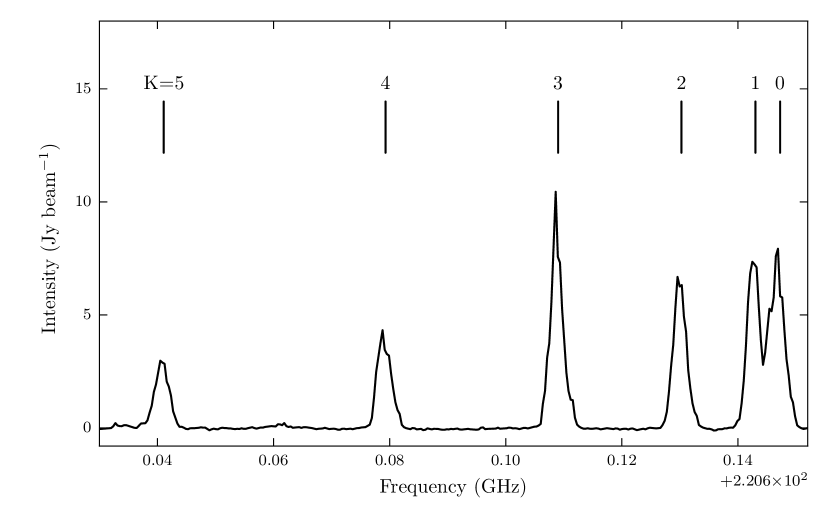
Figure 21: Peak spectrum of the CH₃CN $J=12-11$ observations showing the $K$ transitions.

For the modelling, three nested grids with increasing resolution on the region close to the star were used. The grids were defined with $80^{3}$, $100^{3}$ and $100\times 100\times 50$ cells from large to small scale, respectively. The former covers a size of $4.0\times 10^{5}$ au, the second a grid size of $5.0\times 10^{4}$ au, and the latter a size of 2000 au in the x-y plane. The smallest scale this grid can resolve is 20 au.

In order to evaluate the density, temperature and velocity in these grids, we first oversample each nested grid by dividing each grid cell into 27 smaller grid cells for the two large-scale grids and 125 smaller grid cells for the grid sampling the smaller scales. Then the density and velocity distributions are evaluated at each point and the temperature is interpolated. Finally, number density weighted averages are taken to obtain the coarser grid values. The line width and abundance grids are obtained by evaluating their functions at the positions of the grid. We fixed the inner radius of the gas distributions to half the dust sublimation radius. We do not expect to constrain this inner radius because the resolution of our observations does not allow it.

We used the Ulrich velocity distribution for the envelope, a Keplerian rotation velocity distribution for the disc and a Hubble expansion law for the outflow. The equations and details of the velocity distribution can be found in Appendix B.2.

mollie includes a line width parameter which was set to the sum in quadrature of the thermal speed of sound and a turbulence/non-thermal velocity. The turbulent velocity line width $\Delta v_{\rm nth}$ was varied during the modelling (see below).

Following the studies of other molecules (e.g. Kaźmierczak-Barthel et al., 2015), the methyl cyanide abundance was defined as a step function of the temperature. This approach has also been used for methyl cyanide in other studies (e.g. Johnston et al., 2015) and more generally for many species which freeze out (e.g. Jørgensen et al., 2004). The abundance function is then defined as

$$X_{\rm CH_{3}CN}(T)=\begin{cases}X_{0}&\text{if }\,T<T_{0}\,,\;\mathrm{or}\\ X_{1}&\text{if }\,T>T_{0}\,.\end{cases}$$ (5)

This approximation is consistent with the change in abundance due to thermal desorption of molecules from dust grains in the evolution of hot cores when the temperature increases with time (e.g. Viti et al., 2004). We explored several temperature values to match the extension of the zeroth moment map and the ratios between the $K=2-5$ lines with increasing number of temperature steps from 0 to 2. It was found that one temperature step is enough to explain the observations and limit the number of parameters to fit. The temperature step was fixed to $T_{0}=100$ K and the abundance below this temperature was fixed to $X_{0}=5\times 10^{-12}$. Hence, only $X_{1}$ was varied during the modelling.

To compare the models with the observations, we obtained pv maps for the $K=2-5$ lines at ${\rm PA}=276\degr$ and $6\degr$, i.e. along and perpendicular to the jet axis, and centred in the peak of the zeroth moment map. We use a slit width for the pv maps equal to 3 times the pixel size, i.e. 1.8 arcsec. The pv maps are shown in Fig. 6. Since the observations are not particularly asymmetric, the two position angles allow us to fit the extension of the emitting region. We aligned the spectral axis of the pv maps by matching the centroid of the line at the central position. The average shift for all the lines and models was $-0.69\pm 0.45$ km s^-1. This value is within the errors in $v_{\rm LSR}$ (see above) and equivalent to a systemic velocity of –6 km s^-1. This shift was applied to all the models prior to the comparison with the observations.

Similar to the continuum modelling visual inspection fitting, the best-fitting model was chosen by averaging the ranking of the $\chi^{2}$ of the pv maps. This method was used because both maps are not independent but have a similar number of points. From the observations we estimated the rms $\sigma_{\rm rms}$ from an emission-free region for each channel and use these values as the errors in the $\chi^{2}$ calculation. We masked points corresponding to the position of NOEMA 2 and emission below $5\sigma_{\rm rms}$.

A.3.1 Parameter selection

All the parameters derived from the best-fitting model to the continuum observations were kept unchanged, with the exception of the envelope infall rate. We varied key parameters for the velocity distribution in a grid with values listed in Table 14. Changes in centrifugal radius will not necessarily fit the continuum data because these change the density and temperature distributions. Therefore, the centrifugal radius was not varied. The envelope infall rate was scaled to keep the density of the envelope constant (cf. eq. 6).

Table 14: Values of the line modelling parameter grid.

Parameter	Values
$M_{\star}^{a}$	15, 25, 35 M☉
Abundance ($X_{1}$)b	$(2,2.5,3,3.5,4,4.5)\times 10^{-8}$
Outflow velocityc ($v_{0}$)	0, 1, 5, 10 km s-1
Turbulent width ($\Delta v_{\rm nth}$)	0.5, 0.8, 1.0, 1.5, 2.0 km s-1

^a we report the results for $M_{\star}=35\,\mbox{M${}_{\sun}$}$ and use the other masses for comparison.

^b for $T>100$ K.

^c Defined at $z=10^{4}$ au.

The range of the abundance values is based on the results of the 1-D line modelling (see Section 4.2.1), which in turn are consistent with values in the literature for methyl cyanide in high-mass star-forming regions (e.g Hunter et al., 2014; Johnston et al., 2015; Palau et al., 2017; Ahmadi et al., 2018).

The disc velocity only changed when the stellar mass was varied. The direction of the rotation of the envelope and disc was fixed to $\phi_{\rm dir}=1$, i.e. anticlockwise looking down from the blue-shifted cavity axis as suggested by Wang et al. (2012) from their first moment maps of HDO, H₂¹⁸O and SO₂ line emission.

The outflow velocities were based on Johnston et al. (2013), who found an average velocity relative to $v_{\rm LSR}$ of $-1.2$ km s^-1 at a projected outflow length of 47300 au (i.e. ${\sim}110000$ au at an inclination angle of 25°) from C¹⁸O line observations. Wang et al. (2012) found that a wind with a Hubble law constant of 10 km s^-1 arcsec^-1, which is roughly 5 times higher than the highest velocity used here (10 km s^-1 per 10000 au). Such high-velocity disc wind was not included here because the scale affected by it is not resolved by the methyl cyanide observations. In addition, the wind model used by Wang et al. (2012) is equatorial, i.e. without a velocity component in the polar direction, rather than spherical as our model. It is worth noticing that the methyl cyanide emission does not show any signatures of outflows, thus it is not expected to constrain this parameter.

Appendix B Physical distributions

An extensive list of the parameters used in this section can be found in Tables 11 and 14. In what follows, we use the $(r,\,\theta,\,\phi)$ nomenclature for spherical coordinates and $(R,\,z,\,\phi)$ for cylindrical coordinates.

B.1 Density distribution

The envelope density distribution of types A and B models (see Table 10) use the Ulrich (1976) analytical solution for rotating, infalling material (hereafter Ulrich envelope)

$$\rho(r,\theta)=\frac{\dot{M}_{\mathrm{env}}}{4\pi(GM_{\star}R_{c}^{3})^{0.5}}\left(\frac{r}{R_{c}}\right)^{-1.5}\left(1+\frac{\mu}{\mu_{0}}\right)^{-0.5}\\ \left(\frac{\mu}{\mu_{0}}+\frac{2\mu_{0}^{2}R_{c}}{r}\right)^{-1}\propto\frac{\dot{M}_{\mathrm{env}}}{\sqrt{M_{\star}}}f(\mathbf{r},R_{\mathrm{c}})\,,$$ (6)

where $G$ is the gravitational constant, $f(\mathbf{r},R_{\mathrm{c}})$ is a function of the position and the centrifugal radius, $\mu=\cos\theta$ and $\mu_{0}=\cos\theta_{0}$, with $\theta_{0}$ the angle of the parabolic orbits of the infalling material, and is calculated by solving

$$\mu_{0}^{3}+\mu_{0}\left(\frac{r}{R_{c}}-1\right)-\mu\left(\frac{r}{R_{c}}\right)=0\,.$$ (7)

This density distribution behaves like a power law $n(r)\propto r^{-1.5}$ for distances $r$ larger than the centrifugal radius $R_{\mathrm{c}}$, i.e. like free-falling material, while at shorter distances the density is relatively constant.

Type B models were used to study the MYSO W33A (de Wit et al., 2010), and unlike type A they have an alpha disc (e.g. Shakura & Sunyaev, 1973) with accretion luminosity. The disc density distribution of type A models is given by

$$\rho(R,z)=\rho_{0}\left(\frac{R_{0}}{R}\right)^{\alpha}\exp\left[-0.5\left(\frac{z}{h(R)}\right)^{2}\right]\,,$$ (8)

with the reference density $\rho_{0}$ calculated to match the disc mass ($M_{d}$), a fiducial radius $R_{0}=100\,{\rm au}$ and the scale height $h=h_{0}(R/R_{0})^{\beta}$. The disc density distribution of type B models differs by a factor $(1-\sqrt{R_{\star}/R})$, with $R_{\star}$ the stellar radius, from that of type A models (see hyperion documentation). The disc radius was set to the centrifugal radius $R_{c}$.

Type C is one of the proposed solutions to increase the underestimated near and mid-IR fluxes, which results from 1-D spherically symmetric envelopes used to model SEDs and submm intensity radial profiles of MYSOs (e.g. Williams et al., 2005). The density distribution of this type of models is parametrised as a power law $n=n_{0}(r/r_{0})^{-p}$ with $r_{0}=0.5R_{\mathrm{out}}$, $R_{\mathrm{out}}$ the envelope radius and the density reference value $n_{0}$ is determined by the mass of the envelope $M_{\mathrm{env}}$.

We use the empirical expression found by Whitney et al. (2004) to estimate the dust sublimation radius

$$R_{\mathrm{in}}=R_{\star}\left(\frac{T_{\star}}{T_{\mathrm{sub}}}\right)^{2.1}\propto\sqrt{L_{\star}}\frac{T_{\star}^{0.1}}{T_{\mathrm{sub}}^{2.1}}$$ (9)

where $T_{\mathrm{sub}}$ is the sublimation temperature. For a sublimation temperature $T_{\mathrm{sub}}=1500\,{\rm K}$, luminosity $L_{\star}=1.6\times 10^{5}$ L_☉ and stellar temperatures $T_{\star}=10000-40000$ K the sublimation radius ranges between 30–40 au.

B.2 Velocity distribution

For the envelope, we used the Ulrich envelope velocity distribution. The velocity components of the envelope inside the disc radius were set to zero because the Ulrich solution is undefined at the centrifugal radius resulting in a large increase in velocity. This produces a discontinuity in the velocity distribution but at scales which are not resolved by our observations. The 3-D components of the envelope velocity distribution are given in spherical coordinates by (e.g. Stahler & Palla, 2005)

$$v_{r}(r,\theta)=-\left(\frac{GM_{\star}}{r}\right)^{1/2}\left(1+\frac{\mu}{\mu_{0}}\,,\right)^{1/2}$$ (10)

$$v_{\theta}(r,\theta)=\left(\frac{GM_{\star}}{r}\right)^{1/2}\frac{\mu_{0}-\mu}{\sin\theta}\left(1+\frac{\mu}{\mu_{0}}\right)^{1/2}\,,$$ (11)

$$v_{\phi}(r,\theta)=\phi_{\rm dir}\left(\frac{GM_{\star}}{r}\right)^{1/2}\frac{\sin\theta_{0}}{\sin\theta}\left(1-\frac{\mu}{\mu_{0}}\right)^{1/2}\,,$$ (12)

where $\phi_{\rm dir}$ parametrises the direction of rotation, i.e. has a value of $\pm 1$. We use a stellar mass of 35 M_☉ for the modelling, but as a reference we also calculated models with lower masses.

The outflow velocity was modelled with a Hubble expansion law

$$v_{r}(r)=v_{0}\frac{r}{r_{0}}\,,$$ (13)

where $v_{0}$ is the velocity at $r_{0}=10^{4}\cos^{-1}\theta_{\rm c}$ au with $\theta_{\rm c}$ the half-opening angle of the cavity like in the continuum modelling. A similar velocity distribution was used by Wang et al. (2012) to interpret the molecular emission from the PdBI 1.4 mm observations at a smaller scale, but as a cylindrical radial (i.e. perpendicular to the outflow cavity direction) expansion. A limit of 12 km s^-1 was set to the outflow velocity. Velocities larger than this limit are achieved in colder less dense gas than the envelope, thus its contribution to the spectra is not important.

For the disc, the azimuthal velocity was parametrised as a Keplerian disc, which is described by (e.g. Shakura & Sunyaev, 1976)

$$v_{\phi}(R)=\phi_{\rm dir}\sqrt{\frac{GM_{\star}}{R}}\,,$$ (14)

The other two components of the velocity were set to zero in order to limit the number of parameters in the fit and because the disc is not resolved in the observations.

Appendix C Model image processing

To obtain the data products in Table 5 different processes were used. For images, we have chosen to compare them on a pixel-by-pixel basis by aligning the emission peak. For the UKIRT images, we have used the observed WCS information in the image headers because the peak emission is saturated. The images are convolved with the respective PSF, where we have also taken into account the PSF rotations. To compare the images, they were also masked to isolate the source and exclude emission which cannot be reproduced by our model because of its symmetry. In the $J$, $H$ and $K$ bands this includes features in the outflow cavity (the so-called “loops”), point-like sources inside and outside the cavity and the saturated central region. The diffraction pattern seen in the $K$-band map (see Fig. 7) was not masked.

Monte Carlo noise was present in the images produced by the radiative transfer code because of its probabilistic nature. This noise affected more strongly the near-IR observations due to scattering. In order to reduce this noise in the $JHK$-band images we followed a 2-step process. First, we identified isolated pixels by approximating pixels with fluxes lower than $10^{-10}$ Jy sr^-1 to zero and using a median filter of size 2. This filters out pixels which are located in the outskirts of the cavity and in other similar regions. Then, to recover the pixels in the outskirts of the cavity, we calculated the local density of pixels with values larger than zero within $7\times 7$ pixel² boxes. We used the 75th percentile of the local density values of any given image as threshold so pixels in regions of high local density of pixels, like the outflow cavity, are not filtered out. The amount of flux loss is ${\sim}1$ per cent on average.

A similar procedure was followed to obtain the images used for the model radial intensity profiles. These images were not rotated since the PSF is symmetric and only radial profiles are compared. With these images we follow the same steps utilised to obtain the observed profiles (see Section 2.3.2). In these cases, we have chosen to compare points whose observed intensity is higher than three times the image noise.

In the particular case of the $K$-band speckle interferometric visibilities we Fourier transformed the model image and obtained the visibility radial profile. For the mm interferometric data, we used casa (McMullin et al., 2007) to simulate the observed visibilities from our model images. Noise was added to the simulated observations. For reproducing the observed PSF properties as close as possible, we used the on-source integration time, antenna configurations and hour angle of the observations. The simulated observations have a PSF FWHM of $2\aas@@fstack{\prime\prime}3\times 1\aas@@fstack{\prime\prime}8$ with PA$=93\degr$ and $0\aas@@fstack{\prime\prime}46\times 0\aas@@fstack{\prime\prime}35$ with PA$=62\degr$ in the compact and extended configurations respectively (cf. Table 5). We chose to compare points at uv distances larger than $40\,{\rm k}\lambda$ (angular scale of ${\sim}6$ arcsec) in the compact configuration data because emission not belonging to the core (e.g. background emission from the large scale molecular cloud) may have been included at smaller uv distances. Similarly, we limited the comparison of extended configuration data to uv distances between 100 and $400\,{\rm k}\lambda$ (angular scales between ${\sim}2.5-0.6$ arcsec). Shorter uv distances ($<100\,{\rm k}\lambda$) are covered by the compact configuration and may be underrepresented in the high-resolution model image, whilst larger uv distances ($>400\,{\rm k}\lambda$) may include substructures that the model cannot reproduce (e.g. clumpy emission, see Fig. 3b).

The CH₃CN model images were rotated to match the jet PA and then synthetic observations were calculated with casa. The synthetic images included thermal noise which approximately matches that observed. The $K=3$ line first moment map in Fig. 22(a) shows that, if the velocity structure was completely due to rotation, the rotation axis will be oriented roughly at a ${\rm PA}=286\degr$. However, as pointed out by Wang et al. (2012), expansion or infalling motions can change the perceived position of the rotation angle. The orientation of the disc plane as derived from a Gaussian fit to the 1.3 mm extended configurations map is $\mathrm{PA}=21\degr$, similarly the orientation of the 1.4 mm continuum emission from Wang et al. (2012) is ${\rm PA}=6\degr$. These values are nearly perpendicular to the radio jet orientation (${\rm PA}\sim 100\degr$ from Johnston et al., 2013, see Fig. 5). Therefore, the small scale rotation axis does not have the same orientation as the large scale outflow cavity ($\mathrm{PA}=259\degr$). Then the orientation of the model rotation axis was set to ${\rm PA}=276\degr$, i.e. perpendicular to the disc plane.

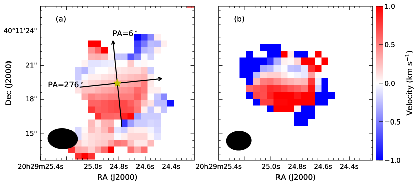
Figure 22: NOEMA compact configuration first moment map for the observed CH₃CN $J=12-11$ $K=3$ line (a) and from the overall best-fitting model (b). Black arrows show the direction of the slices in Fig. 6 with the arrows pointing towards positive offsets. The star marks the position of the radio continuum source. The beam is shown in black in the lower left corner.

Appendix D Best-fitting model by types

Table 15 lists the parameters for the continuum best-fitting models from the visual inspection for types B and C, and from the grid fitting for type A.

Table 15: Parameters of the continuum best-fitting models by density distribution type.

Parameter	Type
	A	B	C
Inclination angle ($i$)	25°	30°	40°
Stellar temperature ($T_{\star}$/K)	18000	18000	30000
Stellar luminosity ($L_{\star}/10^{5}$ L☉)	1.6	1.6	1.4
Outer radius ($R_{\mathrm{out}}$/au)	195000	195000	300000
Envelope infall rate ($\dot{M}_{\mathrm{env}}/10^{-3}\,\mbox{M${}_{\sun}$}\,{\rm yr}^{-1}$)	2.0	1.5a	–
Envelope mass ($M_{\mathrm{env}}/10^{3}\,\mbox{M${}_{\sun}$}$)	2.1b	1.6b	1.0
Envelope dust	OHM92	OHM92	WD01
Centrifugal radius ($R_{\mathrm{c}}$/au)	2200	440	100
Disc mass ($M_{\mathrm{d}}$/M☉)	6.0	1.0	1.2
Disc scale height at $r=100$ au ($h_{0}$/au)	0.6	0.6	0.6
Disc flaring exponent ($\alpha$)	2.25	2.25	2.25
Disc vertical density exponent ($\beta$)	1.25	1.25	1.25
Disc dust	OHM92	OHM92	OHM92
Cavity opening anglec ($2\theta_{\rm cav}$)	60°	56°	60°
Cavity shape exponent ($b_{\mathrm{cav}}$)	2.0	2.0	2.0
Cavity density exponent ($p_{\rm cav}$)	2.0	2.0	2.0
Cavity reference densityc ($\rho_{\rm cav}/10^{-21}$ g cm-3)	1.4	1.4	$3.5\times 10^{-3}$
Cavity dust	KMH	KMH	KMH

^a Scaled to a stellar mass of 35 M_☉.

^b Not an input parameter.

^c Defined at a height $z=10^{4}$ au.

References

- Ahmadi et al. (2018) Ahmadi A., et al., 2018, A&A, 618, A46
- Alvarez et al. (2004) Alvarez C., Hoare M., Lucas P., 2004, A&A, 419, 203
- Benz et al. (2007) Benz A. O., Stäuber P., Bourke T. L., van der Tak F. F. S., van Dishoeck E. F., Jørgensen J. K., 2007, A&A, 475, 549
- Beuther et al. (2018) Beuther H., et al., 2018, A&A, 617, A100
- Boonman et al. (2001) Boonman A. M. S., Stark R., van der Tak F. F. S., van Dishoeck E. F., van der Wal P. B., Schäfer F., de Lange G., Laauwen W. M., 2001, ApJ, 553, L63
- Bruderer et al. (2009) Bruderer S., Benz A. O., Doty S. D., van Dishoeck E. F., Bourke T. L., 2009, ApJ, 700, 872
- Bruderer et al. (2010) Bruderer S., Benz A. O., Stäuber P., Doty S. D., 2010, ApJ, 720, 1432
- Campbell (1984) Campbell B., 1984, ApJ, 287, 334
- Casali et al. (2007) Casali M., et al., 2007, A&A, 467, 777
- Commerçon et al. (2011) Commerçon B., Hennebelle P., Henning T., 2011, ApJ, 742, L9
- Cunningham et al. (2011) Cunningham A. J., Klein R. I., Krumholz M. R., McKee C. F., 2011, ApJ, 740, 107
- Davies et al. (2011) Davies B., Hoare M. G., Lumsden S. L., Hosokawa T., Oudmaijer R. D., Urquhart J. S., Mottram J. C., Stead J., 2011, MNRAS, 416, 972
- Di Francesco et al. (2008) Di Francesco J., Johnstone D., Kirk H., MacKenzie T., Ledwosinska E., 2008, ApJS, 175, 277
- Duarte-Cabral et al. (2013) Duarte-Cabral A., Bontemps S., Motte F., Hennemann M., Schneider N., André P., 2013, A&A, 558, A125
- Gieser et al. (2019) Gieser C., et al., 2019, A&A, 631, A142
- Griffin et al. (2010) Griffin M. J., et al., 2010, A&A, 518, L3
- Haemmerlé & Peters (2016) Haemmerlé L., Peters T., 2016, MNRAS, 458, 3299
- Hasegawa & Mitchell (1995) Hasegawa T. I., Mitchell G. F., 1995, ApJ, 451, 225
- Hatchell et al. (2000) Hatchell J., Fuller G. A., Millar T. J., Thompson M. A., Macdonald G. H., 2000, A&A, 357, 637
- Hoare (2002) Hoare M. G., 2002, in Crowther P., ed., Astronomical Society of the Pacific Conference Series Vol. 267, Hot Star Workshop III: The Earliest Phases of Massive Star Birth. p. 137
- Hoare & Franco (2007) Hoare M. G., Franco J., 2007, Astrophysics and Space Science Proceedings, 1, 61
- Hosokawa et al. (2010) Hosokawa T., Yorke H. W., Omukai K., 2010, ApJ, 721, 478
- Hunter et al. (2014) Hunter T. R., Brogan C. L., Cyganowski C. J., Young K. H., 2014, ApJ, 788, 187
- Izquierdo et al. (2018) Izquierdo A. F., Galván-Madrid R., Maud L. T., Hoare M. G., Johnston K. G., Keto E. R., Zhang Q., de Wit W.-J., 2018, MNRAS, 478, 2505
- Johnston et al. (2013) Johnston K. G., Shepherd D. S., Robitaille T. P., Wood K., 2013, A&A, 551, A43
- Johnston et al. (2015) Johnston K. G., et al., 2015, ApJ, 813, L19
- Jørgensen et al. (2002) Jørgensen J. K., Schöier F. L., van Dishoeck E. F., 2002, A&A, 389, 908
- Jørgensen et al. (2004) Jørgensen J. K., Schöier F. L., van Dishoeck E. F., 2004, A&A, 416, 603
- Kaźmierczak-Barthel et al. (2014) Kaźmierczak-Barthel M., van der Tak F. F. S., Helmich F. P., Chavarría L., Wang K.-S., Ceccarelli C., 2014, A&A, 567, A53
- Kaźmierczak-Barthel et al. (2015) Kaźmierczak-Barthel M., Semenov D. A., van der Tak F. F. S., Chavarría L., van der Wiel M. H. D., 2015, A&A, 574, A71
- Keto & Rybicki (2010) Keto E., Rybicki G., 2010, ApJ, 716, 1315
- Kim et al. (1994) Kim S.-H., Martin P. G., Hendry P. D., 1994, ApJ, 422, 164
- Klassen et al. (2016) Klassen M., Pudritz R. E., Kuiper R., Peters T., Banerjee R., 2016, ApJ, 823, 28
- Kölligan & Kuiper (2018) Kölligan A., Kuiper R., 2018, A&A, 620, A182
- Krumholz et al. (2005) Krumholz M. R., McKee C. F., Klein R. I., 2005, ApJ, 618, L33
- Krumholz et al. (2012) Krumholz M. R., Klein R. I., McKee C. F., 2012, ApJ, 754, 71
- Kuiper & Hosokawa (2018) Kuiper R., Hosokawa T., 2018, A&A, 616, A101
- Kuiper & Yorke (2013) Kuiper R., Yorke H. W., 2013, ApJ, 772, 61
- Kuiper et al. (2010) Kuiper R., Klahr H., Beuther H., Henning T., 2010, ApJ, 722, 1556
- Kuiper et al. (2015) Kuiper R., Yorke H. W., Turner N. J., 2015, ApJ, 800, 86
- Kuiper et al. (2016) Kuiper R., Turner N. J., Yorke H. W., 2016, ApJ, 832, 40
- Lada et al. (1984) Lada C. J., Thronson Jr. H. A., Smith H. A., Schwartz P. R., Glaccum W., 1984, ApJ, 286, 302
- Laor & Draine (1993) Laor A., Draine B. T., 1993, ApJ, 402, 441
- Lucas et al. (2008) Lucas P. W., et al., 2008, MNRAS, 391, 136
- Lumsden et al. (2013) Lumsden S. L., Hoare M. G., Urquhart J. S., Oudmaijer R. D., Davies B., Mottram J. C., Cooper H. D. B., Moore T. J. T., 2013, ApJS, 208, 11
- Lutz (2012) Lutz D., 2012, Herschel Internal Document PICC-ME-TN-03, PACS Photometer Point Spread Function (http://herschel.esac.esa.int/twiki/pub/Public/PacsCalibrationWeb/bolopsf_20.pdf)
- Mathis et al. (1977) Mathis J. S., Rumpl W., Nordsieck K. H., 1977, ApJ, 217, 425
- Matzner & McKee (1999) Matzner C. D., McKee C. F., 1999, ApJ, 526, L109
- Maud et al. (2013) Maud L. T., Hoare M. G., Gibb A. G., Shepherd D., Indebetouw R., 2013, MNRAS, 428, 609
- Maud et al. (2017) Maud L. T., Hoare M. G., Galván-Madrid R., Zhang Q., de Wit W. J., Keto E., Johnston K. G., Pineda J. E., 2017, MNRAS, 467, L120
- McDonald et al. (2011) McDonald M., Courteau S., Tully R. B., Roediger J., 2011, MNRAS, 414, 2055
- McMullin et al. (2007) McMullin J. P., Waters B., Schiebel D., Young W., Golap K., 2007, in Shaw R. A., Hill F., Bell D. J., eds, Astronomical Society of the Pacific Conference Series Vol. 376, Astronomical Data Analysis Software and Systems XVI. p. 127
- Meyer et al. (2018) Meyer D. M. A., Kuiper R., Kley W., Johnston K. G., Vorobyov E., 2018, MNRAS, 473, 3615
- Minchin et al. (1991) Minchin N. R., Hough J. H., McCall A., Aspin C., Hayashi S. S., Yamashita T., Burton M. G., 1991, MNRAS, 251, 508
- Molinari et al. (2010) Molinari S., et al., 2010, PASP, 122, 314
- Morales et al. (2009) Morales E. F. E., Mardones D., Garay G., Brooks K. J., Pineda J. E., 2009, ApJ, 698, 488
- Motte et al. (2007) Motte F., Bontemps S., Schilke P., Schneider N., Menten K. M., Broguière D., 2007, A&A, 476, 1243
- Motte et al. (2010) Motte F., et al., 2010, A&A, 518, L77
- Mottram et al. (2011a) Mottram J. C., et al., 2011a, A&A, 525, A149
- Mottram et al. (2011b) Mottram J. C., et al., 2011b, ApJ, 730, L33
- Myers et al. (2013) Myers A. T., McKee C. F., Cunningham A. J., Klein R. I., Krumholz M. R., 2013, ApJ, 766, 97
- Olguin et al. (2015) Olguin F. A., Hoare M. G., Wheelwright H. E., Clay S. J., de Wit W.-J., Rafiq I., Pezzuto S., Molinari S., 2015, MNRAS, 449, 2784
- Ossenkopf et al. (1992) Ossenkopf V., Henning T., Mathis J. S., 1992, A&A, 261, 567
- Palau et al. (2013) Palau A., Sánchez Contreras C., Sahai R., Sánchez-Monge Á., Rizzo J. R., 2013, MNRAS, 428, 1537
- Palau et al. (2014) Palau A., et al., 2014, ApJ, 785, 42
- Palau et al. (2017) Palau A., et al., 2017, MNRAS, 467, 2723
- Parkin et al. (2009) Parkin E. R., Pittard J. M., Hoare M. G., Wright N. J., Drake J. J., 2009, MNRAS, 400, 629
- Peters et al. (2010) Peters T., Klessen R. S., Mac Low M.-M., Banerjee R., 2010, ApJ, 725, 134
- Peters et al. (2011) Peters T., Banerjee R., Klessen R. S., Mac Low M.-M., 2011, ApJ, 729, 72
- Pilbratt et al. (2010) Pilbratt G. L., et al., 2010, A&A, 518, L1
- Poetzel et al. (1992) Poetzel R., Mundt R., Ray T. P., 1992, A&A, 262, 229
- Poglitsch et al. (2010) Poglitsch A., et al., 2010, A&A, 518, L2
- Preibisch et al. (2003) Preibisch T., Balega Y. Y., Schertl D., Weigelt G., 2003, A&A, 412, 735
- Richer et al. (2000) Richer J. S., Shepherd D. S., Cabrit S., Bachiller R., Churchwell E., 2000, in Mannings V., Boss A. P., Russell S. S., eds, Protostars and Planets IV. p. 867 (arXiv:astro-ph/9904097)
- Robitaille (2011) Robitaille T. P., 2011, A&A, 536, A79
- Robitaille (2017) Robitaille T. P., 2017, A&A, 600, A11
- Rodgers & Charnley (2001) Rodgers S. D., Charnley S. B., 2001, ApJ, 546, 324
- Roy et al. (2011) Roy A., et al., 2011, ApJ, 727, 114
- Roy et al. (2014) Roy A., et al., 2014, A&A, 562, A138
- Russeil et al. (2010) Russeil D., Zavagno A., Motte F., Schneider N., Bontemps S., Walsh A. J., 2010, A&A, 515, A55
- Rygl et al. (2012) Rygl K. L. J., et al., 2012, A&A, 539, A79
- Sadavoy et al. (2013) Sadavoy S. I., et al., 2013, ApJ, 767, 126
- Sanna et al. (2012) Sanna A., Reid M. J., Carrasco-González C., Menten K. M., Brunthaler A., Moscadelli L., Rygl K. L. J., 2012, ApJ, 745, 191
- Schneider et al. (2016) Schneider N., et al., 2016, A&A, 591, A40
- Shakura & Sunyaev (1973) Shakura N. I., Sunyaev R. A., 1973, A&A, 500, 33
- Shakura & Sunyaev (1976) Shakura N. I., Sunyaev R. A., 1976, MNRAS, 175, 613
- Simpson et al. (2013) Simpson J. P., et al., 2013, MNRAS, 435, 3419
- Smith et al. (2009) Smith R. J., Longmore S., Bonnell I., 2009, MNRAS, 400, 1775
- Stahler & Palla (2005) Stahler S. W., Palla F., 2005, The Formation of Stars
- Stäuber et al. (2005) Stäuber P., Doty S. D., van Dishoeck E. F., Benz A. O., 2005, A&A, 440, 949
- Tamura & Yamashita (1992) Tamura M., Yamashita T., 1992, ApJ, 391, 710
- Tobin et al. (2012) Tobin J. J., Hartmann L., Bergin E., Chiang H.-F., Looney L. W., Chandler C. J., Maret S., Heitsch F., 2012, ApJ, 748, 16
- Tofani et al. (1995) Tofani G., Felli M., Taylor G. B., Hunter T. R., 1995, A&AS, 112, 299
- Trinidad et al. (2003) Trinidad M. A., et al., 2003, ApJ, 589, 386
- Trinidad et al. (2013) Trinidad M. A., et al., 2013, MNRAS, 430, 1309
- Ulrich (1976) Ulrich R. K., 1976, ApJ, 210, 377
- Vázquez-Semadeni et al. (2019) Vázquez-Semadeni E., Palau A., Ballesteros-Paredes J., Gómez G. C., Zamora-Avilés M., 2019, arXiv e-prints, p. arXiv:1903.11247
- Viti et al. (2004) Viti S., Collings M. P., Dever J. W., McCoustra M. R. S., Williams D. A., 2004, MNRAS, 354, 1141
- Wang et al. (2012) Wang K.-S., van der Tak F. F. S., Hogerheijde M. R., 2012, A&A, 543, A22
- Weingartner & Draine (2001) Weingartner J. C., Draine B. T., 2001, ApJ, 548, 296
- Whitney et al. (2003) Whitney B. A., Wood K., Bjorkman J. E., Wolff M. J., 2003, ApJ, 591, 1049
- Whitney et al. (2004) Whitney B. A., Indebetouw R., Bjorkman J. E., Wood K., 2004, ApJ, 617, 1177
- Whitney et al. (2013) Whitney B. A., Robitaille T. P., Bjorkman J. E., Dong R., Wolff M. J., Wood K., Honor J., 2013, ApJS, 207, 30
- Williams et al. (2005) Williams S. J., Fuller G. A., Sridharan T. K., 2005, A&A, 434, 257
- Wood et al. (2002) Wood K., Wolff M. J., Bjorkman J. E., Whitney B., 2002, ApJ, 564, 887
- Zhang et al. (2013) Zhang Y., Tan J. C., McKee C. F., 2013, ApJ, 766, 86
- de Wit et al. (2009) de Wit W. J., et al., 2009, A&A, 494, 157
- de Wit et al. (2010) de Wit W. J., Hoare M. G., Oudmaijer R. D., Lumsden S. L., 2010, A&A, 515, A45
- de Wit et al. (2011) de Wit W. J., Hoare M. G., Oudmaijer R. D., Nürnberger D. E. A., Wheelwright H. E., Lumsden S. L., 2011, A&A, 526, L5
- di Folco et al. (2009) di Folco E., Dutrey A., Chesneau O., Wolf S., Schegerer A., Leinert C., Lopez B., 2009, A&A, 500, 1065
- van Dishoeck & Blake (1998) van Dishoeck E. F., Blake G. A., 1998, ARA&A, 36, 317
- van der Tak & Menten (2005) van der Tak F. F. S., Menten K. M., 2005, A&A, 437, 947
- van der Tak et al. (1999) van der Tak F. F. S., van Dishoeck E. F., Evans II N. J., Bakker E. J., Blake G. A., 1999, ApJ, 522, 991
- van der Tak et al. (2006) van der Tak F. F. S., Walmsley C. M., Herpin F., Ceccarelli C., 2006, A&A, 447, 1011
- van der Tak et al. (2007) van der Tak F. F. S., Black J. H., Schöier F. L., Jansen D. J., van Dishoeck E. F., 2007, A&A, 468, 627