A scalable random forest regressor for combining neutron-star equation of state measurements: A case study with GW170817 and GW190425

Abstract

Gravitational-wave observations of binary neutron star coalescences constrain the neutron-star equation of state by enabling measurement of the tidal deformation of each neutron star. This deformation is well approximated by the tidal deformability parameter $\Lambda$, which was constrained using the first binary neutron star gravitational-wave observation, GW170817. Now, with the measurement of the second binary neutron star, GW190425, we can combine different gravitational-wave measurements to obtain tighter constraints on the neutron-star equation of state. In this paper, we combine data from GW170817 and GW190425 to place constraints on the neutron-star equation of state. To facilitate this calculation, we derive interpolated marginalized likelihoods for each event using a machine learning algorithm. These likelihoods, which we make publicly available, allow for results from multiple gravitational-wave signals to be easily combined. Using these new data products, we find that the radius of a fiducial 1.4 $M_{\odot}$ neutron star is constrained to $11.6^{+1.6}_{-0.9}$ km at 90% confidence and the pressure at twice the nuclear saturation density is constrained to $3.1^{+3.1}_{-1.3}\times 10^{34}$ dyne/cm² at 90% confidence. Combining GW170817 and GW190425 produces constraints indistinguishable from GW170817 alone and is consistent with findings from other works.

1 Introduction

Neutron stars are some of the most compact objects found in our Universe with densities in excess of the nuclear saturation density. Such conditions cannot be simulated by Earth-based experiments and so the study of these objects offers a unique way to understand how matter behaves at supranuclear densities. The behaviour of dense matter in neutron stars is determined by the neutron star equation of state. Gravitational-wave observations of binary neutron star coalescences allow us to constrain the neutron star equation of state by measuring the tidal deformability $\Lambda$, which is a result of the mass-quadrupole moment $Q_{ij}$ induced by the tidal field of the companion star (Damour et al., 1992). The first measurement of a binary neutron star coalescence, GW170817 (Abbott et al., 2017), detected by LIGO and Virgo (Aasi et al., 2015; Acernese et al., 2014), placed the first constraints on $\Lambda$ scaled to a 1.4 $M_{\odot}$ neutron star to $\Lambda_{1.4}\leq 800$ at 90% confidence, favouring compact equations of state. This observation was combined with measurements of the mass of PSR J0348+0432 (Antoniadis et al., 2013), to place constraints on the neutron star radius as well as the pressure inside their cores. De et al. (2018) constrained the radius of the neutron stars in GW170817 to $8.9\,\mathrm{km}\leq R\leq 13.2\,\mathrm{km}$ and Abbott et al. (2018) constrained the radius of both neutron stars to $11.9^{+1.4}_{-1.4}$ km and the pressure at twice the nuclear saturation density to $3.5^{+2.7}_{-1.7}\times 10^{34}$ dyne/cm².

Raaijmakers et al. (2020) combined the tidal deformabilities from GW170817 with the heaviest pulsar observed to date, PSR J0740+6620 (Cromartie et al., 2020), and the mass-radius measurement of pulsar PSR J0030+0451 (Riley et al., 2019; Raaijmakers et al., 2019; Miller et al., 2019). Their results are dominated by PSR J0740+6620. Capano et al. (2020) then combined GW170817 and PSR J0030+0451, including information from low-energy nuclear theory constrained by experimental data. Their results find the tightest constraint on the neutron star equation of state, which constrain the radius of a 1.4 $M_{\odot}$ neutron star to $R=11.0^{+0.9}_{-0.6}$ km (90% confidence).

The second gravitational-wave measurement of a binary neutron star, GW190425 (Abbott et al., 2020a), was detected with a signal-to-noise ratio SNR=12.9, significantly lower than GW170817. This event is interesting because the total mass of the binary is significantly heavier than any other double neutron star system (Farrow et al., 2019). The fact that the binary is massive means that the tidal deformability is small and the gravitational-wave data alone cannot technically rule out that any of the objects of the binary is a black hole, though, this would be highly surprising as massive neutron stars (consistent with those of GW190425) are commonly in found in binaries with white dwarfs (Kiziltan et al., 2013). Despite the low SNR of GW190425, it was possible to map the tidal deformabilities of GW170817 to the mass scale of GW190425 in order to constrain the equation of state (Abbott et al., 2020a), but the results are dominated by the prior, meaning that the data are not informative enough to place tighter constraints on the equation of state.

Neutron star-black hole coalescences can also potentially constrain the neutron star equation of state. A candidate for such an event is GW190814 (Abbott et al., 2020b) which is the result of a merger of a $23.2^{+1.1}_{-1.0}$ $M_{\odot}$ black hole with a $2.59^{+0.08}_{-0.09}$ $M_{\odot}$ compact object. It is not clear whether the compact object is the heaviest neutron star or the lightest black hole observed to date. The tidal deformability of the low mass object is uninformative and no electromagnetic counterpart was observed, which is consistent with a black hole or a neutron star due to the extreme mass ratio and distance of this event (Fernández et al., 2020; Morgan et al., 2020). However, we can use the maximum neutron star mass ($m_{\text{TOV}}$) to determine the nature of this object. If the mass of the compact object is greater than $m_{\text{TOV}}$, we can assume it is a black black hole. Current constraints on the neutron star maximum mass from GW170817 tidal-deformability measurements imply $m_{\rm TOV}\lesssim 2.3\,\mathrm{M_{\odot}}$ (Lim & Holt, 2019; Essick et al., 2020), supporting the conclusion that the $m=2.59^{+0.08}_{-0.09}\,\mathrm{M_{\odot}}$ secondary of GW190814 is too massive to be a neutron star. This claim is further strengthened when the GW170817 constraint is combined with equation of state inference results from terrestrial heavy-ion experiments (Fattoyev et al., 2020).

With the increasing number of binary neutron star measurements from gravitational-wave observations and electromagnetic observations, it is important moving forward to have a framework that allows the community to easily combine different measurements constraining the neutron-star equation of state. In Hernandez Vivanco et al. (2019), we highlighted the technical challenges associated with equation-of-state inference using multiple gravitational-wave events. We pointed out that the usual method of releasing posterior samples is not conducive to equation-of-state inference because inference calculations require the computation of line integrals, which in general do not pass through any of the posterior samples. We proposed a new paradigm, which makes use of machine-learning representations of marginal likelihood surfaces. Similar to our method, the work presented in Wysocki et al. (2020) solves the problem of combining gravitational-wave observations to constrain the equation of state by interpolating the marginalised likelihood using either random forest or Gaussian process interpolation. Their method is used to infer the merger rate and mass distribution of neutron stars in addition to the neutron-star equation of state. See also Lackey & Wade (2015); Agathos et al. (2015) for other approaches to stacking gravitational-wave signals for equation-of-state inference. For a different approach to calculating marginal likelihoods, see Pankow et al. (2015); Lange et al. (2018), which use adaptive mesh refinement to calculate marginal likelihoods on a mesh grid as in Abbott et al. (2018).

In this paper, we build on Hernandez Vivanco et al. (2019) to present constraints on the neutron star equation of state obtained from combining the first two binary neutron star gravitational-wave observations, GW170817 and GW190425. We do not include GW190814 in our analysis because it is unlikely that the compact object is a neutron star and, if it is a neutron star, the tidal deformability is uninformative and does not provide any additional constraints to the neutron star equation of state (Abbott et al., 2020b). While combining data from GW170817 and GW190425, we calculate marginalised likelihoods of GW170817 and GW190425 using a machine learning algorithm consisting of a random forest regressor. We make these data products publicly available. This form of data release is useful for equation of state measurements from multiple measurements.

The advantage of the marginalised likelihoods calculated in this study is that they are continuous and can be evaluated at any point of the $(m,\Lambda)$ plane supported by the posterior distributions of GW170817 and GW190425. (This is helpful for evaluating the aforementioned line integrals required for equation-of-state inference.) Additionally, we can adaptively refine the interpolation by calculating the interpolated likelihood with greater density in the intrinsic parameters depending on the data, which allows us to achieve the necessary interpolation accuracy for whatever calculation may be required.

This paper is organised as follows. In Sec. 2, we give an overview of the method we use to combine gravitational-wave observations and explain why interpolating the likelihood distribution solves the problem of combining events using hierarchical Bayesian inference. In Sec. 3 we explain how to use the interpolated likelihoods released in this study. In Sec. 4 we present constraints on the equation of state using the interpolated likelihoods. In Sec. 5 we discuss our results and we conclude in Sec. 6.

2 Method

We follow the method we introduced in Hernandez Vivanco et al. (2019), which presents a solution to the “stacking problem” found in hierarchical Bayesian inference. We briefly explain how our method works in practise as follows.

We start by writing Bayes theorem, where our aim is to obtain a posterior distribution $p(\Upsilon|\vec{d})$ on the hyper-parameters $\Upsilon$ that define the neutron star equation of state.

$$p(\Upsilon|\vec{d})=\frac{{\cal L}(\vec{d}|\Upsilon)\pi(\Upsilon)}{\mathcal{Z}_{\Upsilon}}.$$ (1)

The posterior $p(\Upsilon|\vec{d})$ depends on the hyper-likelihood $\mathcal{L}(\vec{d}|\Upsilon)$, the hyper-prior $\pi(\Upsilon)$ and the evidence $\mathcal{Z}_{\Upsilon}$. Here, the likelihood $\mathcal{L}_{\text{tot}}$ is defined by

$${\cal L}_{\text{tot}}(\vec{d}|\Upsilon)=\prod_{i}^{N}\int d\theta_{i}{\cal L}(d_{i}|\theta_{i})\pi(\theta_{i}|\Upsilon),$$ (2)

where $N$ are the number of gravitational-wave events that we combine and $\theta$ are the parameters that model the properties of a binary neutron star coalescence. Our method can be extended to account for X-ray observations, e.g. by NICER (Miller et al., 2019), by adding another term in the likelihood defined in Equation (2), which would place additional constraints on the mass and radius of neutron stars. However, in this study we focus only on gravitational-wave observations.

It can be shown that the multi-detector likelihood distribution $\mathcal{L}_{\text{tot}}(\vec{d}|\Upsilon)$ can be expressed as  (e.g. Thrane & Talbot, 2019)

$${\cal L}_{\text{tot}}(\vec{d}|\Upsilon)= \prod_{i}^{N}\frac{\mathcal{Z}_{\emptyset}^{i}}{n_{i}}\sum_{k}^{n_{i}}\frac{\pi(\theta_{i}^{k}|\Upsilon)}{\pi(\theta_{i}^{k}|\emptyset)},$$ (3)

where $n_{i}$ are the posterior samples obtained from running parameter estimation on individual events using an initial prior $\pi(\theta_{i}^{k}|\emptyset)$ and $\pi(\theta_{i}^{k}|\Upsilon)$ is the hyper-prior that depends on hyper-parameters $\Upsilon$ that model the neutron star equation of state.

The stacking problem occurs when we try to combine posterior samples to probe deterministic curves represented in the hyper-prior $\pi(\theta_{i}^{k}|\Upsilon)$, i.e, curves that are infinitely thin instead of having a probability distribution spanning over an area of the parameter space. Since the equation of state is defined by a curve in the $(\Lambda,m)$ plane, we find that no posterior sample will fall exactly on the curve defined by the equation of state and Equation (3) evaluates to zero.

We solve this issue in Hernandez Vivanco et al. (2019) by interpolating the marginalised likelihood for each gravitational-wave observation. This is different to using kernel density estimation (KDE) to represent posterior samples, as in  (e.g. Lackey & Wade, 2015; Raaijmakers et al., 2020), because KDEs perform density estimation whereas likelihood interpolation is a direct surrogate for the underlying function. The marginalised likelihood depends on the intrinsic parameters $\omega=(m_{1},m_{2},\Lambda_{1},\Lambda_{2})$ that determine the neutron star equation of state. By marginalising the likelihood, we can rewrite the total likelihood defined in Equation (2) as

$${\cal L}_{\text{tot}}(\vec{d}|\Upsilon)= \prod_{i}^{N}\int d\omega_{i}{\cal L}_{\kappa}^{\text{int}}(d_{i}|\omega_{i})\pi(\omega_{i}|\Upsilon),$$ (4)

where ${\cal L}_{\kappa}^{\text{int}}(d_{i}|\omega_{i})$ is the interpolated likelihood marginalised over the parameters $\kappa$ that are not in $\omega$.

The interpolated likelihood is obtained by running parameter estimation with parameters $\omega$ fixed at random interpolation points $\omega_{i}$, where we obtain evidences $\mathcal{Z}_{i}$ that effectively represent the marginalised likelihood evaluated at $\omega_{i}$. The data generated during this step is used to train a random forest regressor (Breiman, 2001) to predict the marginalised likelihood at any point $\mathcal{L}(d|\omega_{i})$. We refer to this step as “second-stage parameter estimation”. By working with the interpolated likelihood defined in Equation (4), we do not work with posterior samples at any point and we avoid the issue found in Equation (3).

2.1 Second-stage parameter estimation

To obtain the interpolation likelihood distributions defined in Equation (4), we run parameter estimation by fixing random intrinsic parameters $\omega_{i}=(\mathcal{M}_{i},q_{i},\Lambda_{1,i},\Lambda_{2,i})$, where $\mathcal{M}$ is the chirp mass and $q$ is the mass ratio, to evaluate the marginalised likelihood distribution evaluated at $\omega_{i}$. We refer to this step as “second-stage parameter estimation”. The values of $\omega_{i}$ are chosen from the posterior distributions of each event as well as random points from the prior. We run second-stage parameter estimation with Bilby (Ashton et al., 2019) using the Dynesty sampler (Speagle, 2020). There are some subtleties when running second-stage parameter estimation which we detail below.

The duration of binary neutron star signals is in the order of minutes. Running parameter estimation of binary neutron star inspirals is therefore more computationally expensive than lower-duration events such as binary black hole coalescences. One of the solutions to this problem is to use reduced-order models (ROM) (Smith et al., 2016). The key idea of this method is to remove redundant evaluations of the waveform at some frequency bins, which enables the evaluation of significantly cheaper Bayesian probability distributions using reduced order quadrature (ROQ) integration. This can accelerate Bayesian parameter estimation by as much as a factor of 300 compared to running parameter estimation using the full waveform approximant.

In our analysis, we run second-stage parameter estimation on GW190425 using an ROQ implementation of the precessing-spin waveform approximant IMRPhenomPv2_NRTidal (Khan et al., 2016; Baylor et al., 2019) starting at a frequency $f_{\text{min}}=19.4$ Hz. Similarly, we analyse GW170817 using an ROQ implementation of the spin-aligned waveform approximant IMRPhenomD_NRTidal (Husa et al., 2016; Dietrich et al., 2017) starting at a frequency $f_{\text{min}}=32$ Hz. We do not use the same waveform approximant for GW170817 and GW190425 because we do not currently have an ROQ implementation of the IMRPhenomPv2_NRTidal approximant spanning over the chirp mass values defined by the GW170817 prior. In both cases, we assume a low-spin prior as detailed in Table 1 and Table 2. Note that the minimum frequency at which we start the analyses of both events is different. The reason why we analyse GW170817 from 32 Hz is related to discontinuities in the waveform that break the requirement for the greedy basis finding algorithm defined in Smith et al. (2016), that require the model be smooth. However, when we analyse GW170817 from 32 Hz, contrary to $23$ Hz as in Romero-Shaw et al. (2020b), we lose a signal-to-noise ratio of $\sim 1$. This does not affect the information about the tidal deformabilities, consistent with Harry & Hinderer (2018), but the chirp mass posterior distribution changes from $\mathcal{M}_{\text{23 Hz}}=1.19755^{+0.00012}_{-0.00011}$ to $\mathcal{M}_{\text{32 Hz}}=1.19751^{+0.00020}_{-0.00017}$ (90% confidence) and the lower mass ratio limit changes from $q_{\text{23 Hz}}=0.759$ to $q_{\text{32 Hz}}=0.750$ (90% confidence).

Parameter	Unit	Prior	Minimum	Maximum
$\mathcal{M}$	$M_{\odot}$	Uniform	1.18	1.21
$q$	-	Uniform	0.125	1
$\Lambda_{1}$, $\Lambda_{2}$	-	Uniform	0	5000
$a_{1}$, $a_{2}$	-	Uniform	0	0.05
$\cos(\theta_{jn})$	-	Uniform	-1	1
$\psi$	rad.	Uniform	0	$\pi$
$\phi$	rad.	Uniform	0	$2\pi$
$d_{L}$	Mpc	Comoving	1	75

Table 1: Prior distributions used in the analysis of GW170817. In this table, $\mathcal{M}$ is the chirp mass, $q$ is the mass ratio, $\Lambda_{1,2}$ are the tidal deformabilities, $a_{1,2}$ are the spin magnitudes, $\theta_{jn}$ is the inclination angle, $\psi$ is the polarization angle, $\phi$ is the binary phase and $d_{L}$ is the luminosity distance. We fix the right ascension (RA) and declination (DEC) to 3.44616 and -0.408084 degrees respectively consistent with electromagnetic observations and we use an aligned-spin prior.

Parameter	Unit	Prior	Minimum	Maximum
$\mathcal{M}$	$M_{\odot}$	Uniform	1.485	1.49
$q$	-	Uniform	0.125	1
$\Lambda_{1}$, $\Lambda_{2}$	-	Uniform	0	5000
$a_{1}$, $a_{2}$	-	Uniform	0	0.05
$\theta_{1}$, $\theta_{2}$	rad	Sin	0	$\pi$
$\phi_{12}$, $\phi_{jl}$	rad	Uniform	0	$2\pi$
RA	rad.	Uniform	0	$2\pi$
DEC	rad.	Cos	$-\pi/2$	$\pi/2$
$\cos(\theta_{jn})$	-	Uniform	-1	1
$\psi$	rad.	Uniform	0	$\pi$
$\phi$	rad.	Uniform	0	$2\pi$
$d_{L}$	Mpc	Comoving	1	500

Table 2: Prior distributions used in the analysis of GW190425. The parameters are the same as Table 1 with the difference that we use a precessing-spin prior.

3 Marginalised likelihood fits

3.1 Validation

The key idea of our work is to obtain marginalised likelihood distributions for individual gravitational-wave observations to avoid the stacking problem. We interpolate the likelihood distribution with a random forest regressor (Breiman, 2001) using the Python package Scikit-learn (Pedregosa et al., 2011). A random forest is a bagging algorithm that combines the results from random decision trees to make a prediction. Each tree is trained individually and there is no interaction between each decision tree during training. The results are obtained by averaging the outcomes of each tree which reduces the risk of over-fitting (Biau & Scornet, 2016). In this study, we use 50 decision trees to train our model. Once the model is trained, we use it to predict the marginalised likelihood $\mathcal{L}$, given intrinsic parameters $w=(\mathcal{M},q,\Lambda_{1},\Lambda_{2})$. We generate $\sim 6\times 10^{3}$ interpolation points for GW190425 and $\sim 11\times 10^{3}$ interpolation points for GW170817. We use 90% of this data for training and 10% for testing.

To check if an interpolated marginalised likelihood reproduces the original posterior, we sample the interpolated marginalised likelihood and check if the posterior distributions are consistent. We do this for GW170817 and GW190425. The results are shown in Fig. 1 and Fig. 2, where we see that the interpolated likelihoods accurately reproduce the original posteriors. To quantitatively determine if both distributions are similar, we use the Jensen–Shannon (JS) divergence (Lin, 1991). In Romero-Shaw et al. (2020b), it was found that posteriors with JS divergence values $\gtrsim 0.002$ bit are statistically significant. This value is somewhat arbitrary: Romero-Shaw et al. (2020b) compared a large set of posteriors from multiple gravitational-wave events and demonstrated that a JS divergence of $\lesssim 0.002$ bit results in consistent posteriors, i.e., the median and confidence intervals are essentially the same. For consistency, in this paper, we adopt the threshold value of 0.002 bit proposed in Romero-Shaw et al. (2020b) to compare the original posteriors and the posteriors obtained from sampling the interpolated likelihood. We calculate the JS values for all four intrinsic parameters $\omega=(\mathcal{M},q,\Lambda_{1},\Lambda_{2})$ and find that the maximum JS values for GW190425 and GW170817 are 0.001 bit and 0.002 bit respectively, validating the accuracy of our interpolated likelihoods.

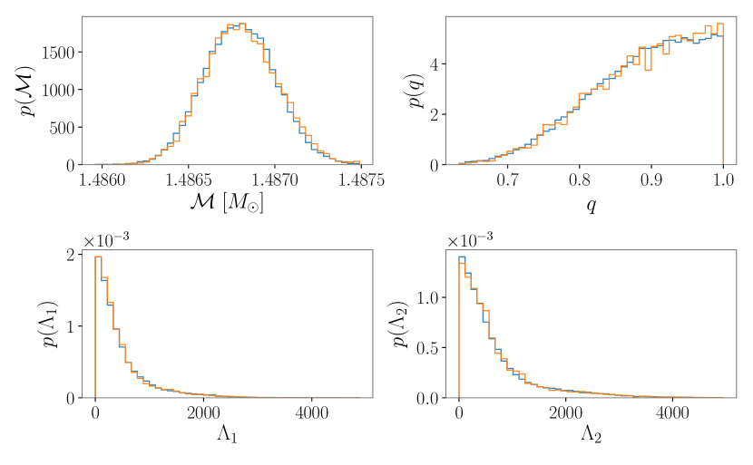
Figure 1: Posterior distributions comparing the original posterior samples from GW190425, shown in blue, with the samples obtained from the interpolated likelihood, shown in orange.

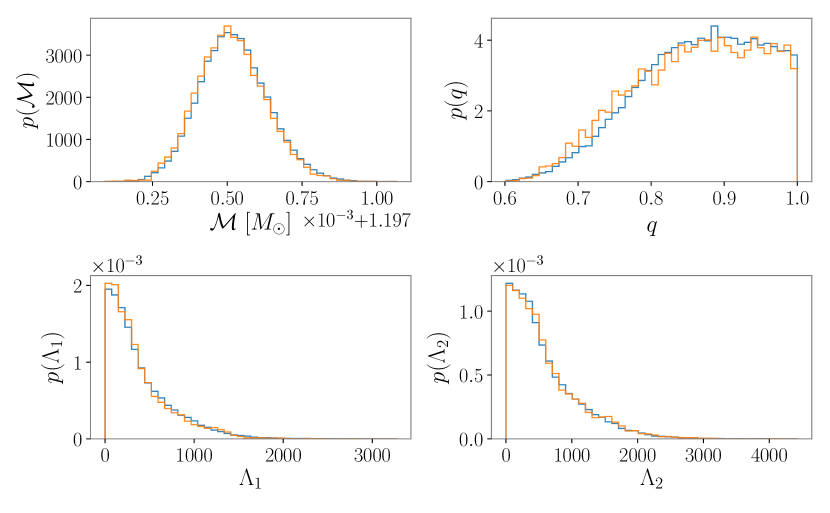
Figure 2: Posterior distributions comparing the original posterior samples from GW170817, shown in blue, with the samples obtained from the interpolated likelihood, shown in orange.

3.2 Data release

We make the GW170817 and GW190425 interpolated marginalised likelihoods publicly available. These likelihoods can be used to reproduce the posteriors shown in Fig. 1 and Fig. 2. This form of data release is potentially more useful than releasing posterior samples alone, as is usually done (e.g. Abbott et al., 2019b; De et al., 2019; Abbott et al., 2019a; Romero-Shaw et al., 2020b). While posterior samples can be used in hierarchical Bayesian inference as long as Equation 3 can be evaluated  (e.g. Talbot & Thrane, 2018; Smith et al., 2020), we cannot use posterior samples alone to constrain the neutron star equation of state without relying on KDE-based methods, as explained in Sec. 2. An interpolated likelihood, on the other hand, can be evaluated at any point of the $(m,\Lambda)$ parameter space and is therefore ideal for use when sampling equation of state hyper-parameters. Moreover, our trained models are fast to evaluate, with a single likelihood evaluation taking in the order of $\sim 6$ ms.

The interpolated marginalised likelihoods can be found in our neuTrOn stAr STacking package, Toast. Our Python package uses a random forest regressor to predict the log likelihood. However, other interpolation methods could improve the accuracy of a random forest regressor. Therefore the interpolation points of GW170817 and GW190425 are also publicly available.

4 Case study: combined equation of state measurement on GW170817 and GW190425

We carry out hierarchical Bayesian inference following the method described in  Hernandez Vivanco et al. (2019). We combine data from GW170817 and GW190425 assuming that both events are the result of binary neutron star coalescences following the same equation of state. We assume the piecewise polytrope parametrisation of the equation of state (Read et al., 2009), which models pressure $p$ as a function of density $\rho$ with three different polytropes. Each polytrope has the form

$$p=K\rho^{\Gamma}.$$ (5)

To fully determine the equation of state with three polytropes, we use four hyper-parameters $\Upsilon=\{\log_{10}p_{0},\Gamma_{1},\Gamma_{2},\Gamma_{3}\}$, where $\log_{10}p_{0}$ is a reference pressure and $\Gamma_{i}$ represents the slope of each polytrope. To convert the gravitational-wave measurable parameters $(m,\Lambda)$ to $(p,\rho)$, we solve the Tolman-Volkoff-Oppenheimer (TOV) equations along with the second Love number $k_{2}$ (Lattimer & Prakash, 2001; Hinderer, 2008) using the LIGO Algorithm Library LALSuite (LIGO Scientific Collaboration, 2018).

While sampling the piecewise polytrope hyper-parameters $\Upsilon$, we impose three conditions:

1. The equation of state must be monotonic, i.e. $dp/d\rho\geq 0$.

2. We require all samples to satisfy that $m_{\text{TOV}}\geq 1.97$ $M_{\odot}$, consistent with pulsars PSR J0348+0432 (Antoniadis et al., 2013) and PSR J0740+6620 (Cromartie et al., 2020).

3. The speed of sound $v_{s}$ should not exceed the speed of light $c$. In practice we, set the restriction to $v_{s}\leq 1.1c$ due to errors introduced by the equation of state parametrisation, as in  Lackey & Wade (2015); Carney et al. (2018).

Using the conditions detailed above, we combine GW170817 and GW190425 by sampling the hyper-parameters $\Upsilon$ using the Bayesian inference library for gravitational-wave astronomy Bilby (Ashton et al., 2019). We use the posterior samples of $\Upsilon$ to obtain posterior samples for $p(\rho)$ and $m(R)$. Our results are shown in Fig. 3. We find that the neutron star radius at a mass of 1.4 $M_{\odot}$ is constrained to $11.6^{+1.6}_{-0.9}$ km at 90% confidence and the pressure at $2\rho_{\text{nuc}}$ ($6\rho_{\text{nuc}}$) saturation density is constrained to $3.1^{+3.1}_{-1.3}\times 10^{34}$ dyne/cm² ($8.3^{+8.6}_{-2.6}\times 10^{35}$ dyne/cm²) at 90% confidence. The results obtained by combining GW170817 and GW19045 are indistinguishable from the constraints of GW170817 alone at the precision given and are consistent with  Abbott et al. (2018, 2020a).

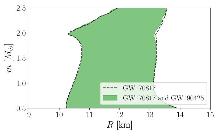
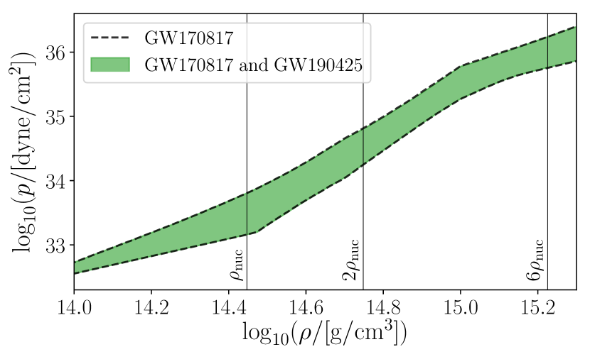
Figure 3: 90% confidence intervals of the posterior distributions of $m(R)$ and $p(\rho)$ obtained by combining GW170817 and GW190425. The neutron star radius at a mass of 1.4 $M_{\odot}$ is constrained to $11.6^{+1.6}_{-0.9}$ km at 90% confidence and the pressure at $2\rho_{\text{nuc}}$ ($6\rho_{\text{nuc}}$) is constrained to $3.1^{+3.1}_{-1.3}\times 10^{34}$ dyne/cm² ($8.3^{+8.6}_{-2.6}\times 10^{35}$ dyne/cm²) at 90% confidence. Our results are dominated by GW170817.

5 Discussion

Abbott et al. (2018) showed that GW170817 constrains the pressure at $2\rho_{\text{nuc}}$ ($6\rho_{\text{nuc}}$) to $3.5^{+2.7}_{-1.7}\times 10^{34}$ dyne/cm² ($9.0^{+7.9}_{-2.6}\times 10^{35}$ dyne/cm²) at 90% confidence. Similarly, GW190425 constrains the pressure at $2\rho_{\text{nuc}}$ ($6\rho_{\text{nuc}}$) to $5.9^{+4.9}_{-3.1}\times 10^{35}$ dyne/cm² ($9.4^{+13.3}_{-4.2}$ dyne/cm²) at 90% confidence (Abbott et al., 2020a). Both of these results are obtained assuming the binaries consist of two neutron stars with the same equation of state, assuming a low-spin prior and setting a maximum neutron-star mass prior to $m_{\text{TOV}}\geq 1.97$ $M_{\odot}$.

Using our method and the same assumptions for the analysis of GW170817 and GW190425, we find that the pressure at $2\rho_{\text{nuc}}$ ($6\rho_{\text{nuc}}$) is constrained to $3.1^{+3.1}_{-1.3}\times 10^{34}$ dyne/cm² ($8.3^{+8.6}_{-2.6}\times 10^{35}$ dyne/cm²) at 90% confidence, consistent with the results presented in Abbott et al. (2017, 2020a). Furthermore, we place limits on the radius of a 1.4 $M_{\odot}$ neutron star to $11.6^{+1.6}_{-0.9}$ km at 90% confidence. De et al. (2018) infer a neutron star radius in the range $8.9\text{ km}\leq R\leq 13.2\text{ km}$ from GW170817, assuming different mass priors and a piecewise polytrope parametrization of the equation of state. Similarly, Essick et al. (2020) find that the radius at a mass of $1.4$ $M_{\odot}$ is constrained to $10.86^{+2.04}_{-1.86}$ km ($12.51^{+1.00}_{-0.88}$ km) with nonparametric priors loosely (tightly) constrained from equations of state found in the literature (Landry & Essick, 2019). Finally, Dietrich et al. (2020) constrain the radius of a 1.4 $M_{\odot}$ neutron star to $11.74^{+0.98}_{-0.79}$ km (90% confindence) by combining GW170817 with its electromagnetic counterparts GRB170817A and AT2017gfo along with NICER measurements, GW190425 and nuclear-physics constraints. Our results are consistent with Abbott et al. (2018); De et al. (2018); Abbott et al. (2020a); Essick et al. (2020); Dietrich et al. (2020).

Although the results from  Abbott et al. (2018); De et al. (2018); Essick et al. (2020) are obtained by analysing GW170817 alone, these are consistent with our results obtained from combining GW170817 and GW190425 because the posteriors are dominated by GW170817. This is consistent with  Hernandez Vivanco et al. (2019), where it was found that the constraints on the equation of state are dominated by events with SNR $\gtrsim 20$.

6 Conclusions

We constrain the neutron star equation of state by combining the gravitational-wave measurements of GW170817 and GW190425. To do so, we calculate interpolated marginalised likelihoods for both events using a random forest regressor. The interpolated likelihoods of GW170817 and GW190425 are made public and we argue that this form of data release is more useful than releasing posterior samples alone. Using the interpolated likelihoods calculated in this study, we find that the radius of a 1.4 $M_{\odot}$ neutron star is constrained to $11.6^{+1.6}_{-0.9}$ km at 90% confidence and the pressure at $2\rho_{\text{nuc}}$ ($6\rho_{\text{nuc}}$) is constrained to $3.1^{+3.1}_{-1.3}\times 10^{34}$ dyne/cm² ($8.3^{+8.6}_{-2.6}\times 10^{35}$ dyne/cm²) at 90% confidence, consistent with results found in the literature.

References

- Aasi et al. (2015) Aasi J., et al., 2015, Class. Quant. Grav., 32, 074001
- Abbott et al. (2017) Abbott B. P., et al., 2017, Phys. Rev. Lett., 119, 161101
- Abbott et al. (2018) Abbott B. P., et al., 2018, Phys. Rev. Lett., 121, 161101
- Abbott et al. (2019a) Abbott R., et al., 2019a, preprint (arXiv:1912.11716)
- Abbott et al. (2019b) Abbott B. P., et al., 2019b, Phys. Rev. X, 9, 031040
- Abbott et al. (2020a) Abbott B. P., et al., 2020a, ApJ, 892, L3
- Abbott et al. (2020b) Abbott R., et al., 2020b, ApJ, 896, L44
- Acernese et al. (2014) Acernese F., et al., 2014, Class. Quant. Grav., 32, 024001
- Agathos et al. (2015) Agathos M., Meidam J., Del Pozzo W., Li T. G. F., Tompitak M., Veitch J., Vitale S., Van Den Broeck C., 2015, Phys. Rev. D, 92, 023012
- Antoniadis et al. (2013) Antoniadis J., et al., 2013, Science, 340, 1233232
- Ashton et al. (2019) Ashton G., et al., 2019, ApJS, 241, 27
- Baylor et al. (2019) Baylor A., Smith R., Chase E., 2019, IMRPhenomPv2_NRTidal_GW190425_narrow_Mc, doi:10.5281/zenodo.3478659
- Biau & Scornet (2016) Biau G., Scornet E., 2016, TEST, 25, 197
- Breiman (2001) Breiman L., 2001, Machine Learning, 45, 5
- Capano et al. (2020) Capano C. D., et al., 2020, Nature Astronomy, 4, 625
- Carney et al. (2018) Carney M. F., Wade L. E., Irwin B. S., 2018, Phys. Rev. D, 98, 063004
- Cromartie et al. (2020) Cromartie H. T., et al., 2020, Nature Astronomy, 4, 72
- Damour et al. (1992) Damour T., Soffel M., Xu C., 1992, Phys. Rev. D, 45, 1017
- De et al. (2018) De S., Finstad D., Lattimer J. M., Brown D. A., Berger E., Biwer C. M., 2018, Phys. Rev. Lett., 121, 091102
- De et al. (2019) De S., Biwer C. M., Capano C. D., Nitz A. H., Brown D. A., 2019, Scientific Data, 6, 81
- Dietrich et al. (2017) Dietrich T., Bernuzzi S., Tichy W., 2017, Phys. Rev. D, 96, 121501
- Dietrich et al. (2020) Dietrich T., Coughlin M. W., Pang P. T. H., Bulla M., Heinzel J., Issa L., Tews I., Antier S., 2020, preprint (arXiv:2002.11355)
- Essick et al. (2020) Essick R., Landry P., Holz D. E., 2020, Phys. Rev. D, 101, 063007
- Farrow et al. (2019) Farrow N., Zhu X.-J., Thrane E., 2019, ApJ, 876, 18
- Fattoyev et al. (2020) Fattoyev F. J., Horowitz C. J., Piekarewicz J., Reed B., 2020, preprint (arXiv:2007.03799)
- Fernández et al. (2020) Fernández R., Foucart F., Lippuner J., 2020, MNRAS, 497, 3221
- Harry & Hinderer (2018) Harry I., Hinderer T., 2018, Class. Quant. Grav., 35, 145010
- Hernandez Vivanco et al. (2019) Hernandez Vivanco F., Smith R., Thrane E., Lasky P. D., Talbot C., Raymond V., 2019, Phys. Rev. D, 100, 103009
- Hinderer (2008) Hinderer T., 2008, ApJ, 677, 1216
- Husa et al. (2016) Husa S., Khan S., Hannam M., Pürrer M., Ohme F., Forteza X. J., Bohé A., 2016, Phys. Rev. D, 93, 044006
- Khan et al. (2016) Khan S., Husa S., Hannam M., Ohme F., Pürrer M., Forteza X. J., Bohé A., 2016, Phys. Rev. D, 93, 044007
- Kiziltan et al. (2013) Kiziltan B., Kottas A., Yoreo M. D., Thorsett S. E., 2013, ApJ, 778, 66
- LIGO Scientific Collaboration (2018) LIGO Scientific Collaboration 2018, LIGO Algorithm Library - LALSuite, free software (GPL), doi:10.7935/GT1W-FZ16
- Lackey & Wade (2015) Lackey B. D., Wade L., 2015, Phys. Rev. D, 91, 043002
- Landry & Essick (2019) Landry P., Essick R., 2019, Phys. Rev. D, 99, 084049
- Lange et al. (2018) Lange J., O’Shaughnessy R., Rizzo M., 2018, preprint (arXiv:1805.10457)
- Lattimer & Prakash (2001) Lattimer J. M., Prakash M., 2001, ApJ, 550, 426
- Lim & Holt (2019) Lim Y., Holt J. W., 2019, Eur. Phys. J. A, 55, 209
- Lin (1991) Lin J., 1991, IEEE Transactions on Information Theory, 37, 145
- Miller et al. (2019) Miller M. C., et al., 2019, ApJ, 887, L24
- Morgan et al. (2020) Morgan R., et al., 2020, ApJ, 901, 83
- Pankow et al. (2015) Pankow C., Brady P., Ochsner E., O’Shaughnessy R., 2015, Phys. Rev. D, 92, 023002
- Pedregosa et al. (2011) Pedregosa F., et al., 2011, J. Mach. Learn. Res., 12, 2825
- Raaijmakers et al. (2019) Raaijmakers G., et al., 2019, ApJ, 887, L22
- Raaijmakers et al. (2020) Raaijmakers G., et al., 2020, ApJ, 893, L21
- Read et al. (2009) Read J. S., Lackey B. D., Owen B. J., Friedman J. L., 2009, Phys. Rev. D, 79, 124032
- Riley et al. (2019) Riley T. E., et al., 2019, ApJ, 887, L21
- Romero-Shaw et al. (2020a) Romero-Shaw I. M., Farrow N., Stevenson S., Thrane E., Zhu X.-J., 2020a, MNRAS, 496, L64
- Romero-Shaw et al. (2020b) Romero-Shaw I. M., et al., 2020b, MNRAS, in press
- Safarzadeh et al. (2020) Safarzadeh M., Ramirez-Ruiz E., Berger E., 2020, ApJ, 900, 13
- Smith et al. (2016) Smith R., Field S. E., Blackburn K., Haster C.-J., Pürrer M., Raymond V., Schmidt P., 2016, Phys. Rev. D, 94, 044031
- Smith et al. (2020) Smith R. J. E., Talbot C., Hernandez Vivanco F., Thrane E., 2020, MNRAS, 496, 3281
- Speagle (2020) Speagle J. S., 2020, MNRAS, 493, 3132
- Talbot & Thrane (2018) Talbot C., Thrane E., 2018, ApJ, 856, 173
- Thrane & Talbot (2019) Thrane E., Talbot C., 2019, PASA, 36, e010
- Wysocki et al. (2020) Wysocki D., O’Shaughnessy R., Wade L., Lange J., 2020, preprint (arXiv:2001.01747)