Theory of oblique-field magnetoresistance from spin centers in three-terminal spintronic devices

Abstract

We present a general stochastic Liouville theory of electrical transport across a barrier between two conductors that occurs via sequential hopping through a single defect’s spin-$0$ to spin-$1/2$ transition.We find magnetoconductances similar to Hanle features (pseudo-Hanle features) that originate from Pauli blocking without spin accumulation, and also predict that evolution of the defect’s spin modifies the conventional Hanle response, producing an inverted Hanle signal from spin center evolution. We propose studies in oblique magnetic fields that would unambiguously determine if a magnetoconductance results from spin-center assisted transport.

Introduction.— A current flowing through a magnetic conductor, with carriers flowing into (spin injection) or out of (spin extraction) a nonmagnetic conductor, can produce a nonequilibrium spin population in the nonmagnetic materialJohnson and Silsbee (1985) that can be sensed through a spin-sensitive voltage. An applied magnetic field, intended to precess these nonequilibrium spins and thereby reduce the voltage (the Hanle effect or HEJohnson and Silsbee (1988)), often produces surprising results challenging to interpret using reasonable spin coherence timesTran et al. (2009); Jansen et al. (2012); Txoperena et al. (2013); Inoue et al. (2015); Txoperena and Casanova (2016). Anomalous Hanle features (the inverted Hanle effect or IHE) were found with parallel applied field and magnetization; conventional interpretations attribute IHE to magnetic fringe fields from a non-uniform interface, however detailed structural measurements of the interface failed to correlate these features with measured non-uniformity. For currents and voltages measured using the same contact (three-terminal, or 3T measurements), features mimicking the HE and IHE were foundTxoperena et al. (2014); Inoue et al. (2015), originating from magnetic-field-dependent transport through spin centers. However, agreement between some 3T and four-terminal (4T) non-local experiments indicates that the impurity effect does not always dominate over direct tunneling Lou et al. (2006, 2007); Aoki et al. (2012).

Here we analyze sequential spin-center-mediated tunneling between different magnetic or non-magnetic leads in both the spin injection and spin extraction regimes using the stochastic Liouville equation (SLE) formalism. The SLE framework is highly adaptable to many physical systems, including spin-oriented tunneling through spin centersHarmon and Flatté (2018). We apply the formalism to sequential tunneling involving a spin center that alternates between spin zero and spin one-half as its charge state changes. In the spin extraction regime, our formalism confirms previous studies that demonstrated supposed HE and IHE to be the result of a Pauli blockade Song and Dery (2014); Inoue et al. (2015), which we now refer to as “pseudo HE” and “pseudo IHE” phenomena. To indicate the experimental geometry without assigning a mechanism we refer to “Hanle measurements” or “inverted Hanle measurements”. The combined effects of spin accumulation at the spin center and the coherent evolution of that spin accumulation lead to an altered spin injection process; we predict a previously undescribed, broad IHE (with same physical origin as the conventional HE) accompanying the known conventional HE (that can be broad or narrow). We will refer to these as “conventional HE” and “conventional IHE”, distinct from the pseudo HE and pseudo IHE. We analyze the oblique field data of Ref. He et al., 2016 to show that a ratio of the angular dependent responses could, in principle, provide incontrovertible evidence of the impurity model by definitively ruling out the fringe-field mechanism for the inverted signal. Our calculations predict distinct magnetic field widths in the magneto-response that motivate further measurements to resolve the origin of the observed features.Lastly we show that the effects described herein require charge current and are thus not present for non-local (4T) measurements (or spin pumping).

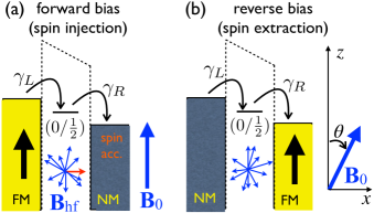
Figure 1: Spin center-mediated transport between a ferromagnet (FM) and nonmagnetic metal (NM) for (a) spin injection and (b) spin extraction with interfacial spin centers possessing a transition level (0/$\frac{1}{2}$). The barrier trap in (a) is a spin transport center. The barrier trap in (b) is a spin bottleneck center. The IHE emerges from (a). If the spin center possesses a nuclear spin moment, assumed to be randomly oriented, some portion (red arrow in (a)) of the hyperfine field will be perpendicular to $\bm{B}_{0}$. This $\perp\bm{B}_{0}$ component reduces the spin current; increasing $B_{0}$ reduces the relative importance of $B_{hf}$ which leads to increasing spin accumulation in the NM. (b) The applied magnetic field makes an angle $\theta$ with respect to the $z$-axis as shown in (b).

Interfacial Spin Centers.— This work treats spin injection and spin extraction between a non-magnetic material (NM) and a ferromagnet (FM); the charge and/or spin current passes through an interfacial barrier trap state through sequential hopping from one lead onto the trap, and then from the trap to the other lead. Figure 1(a) shows spin injection under a forward bias. The transition level of the spin center within the insulating barrier is labeled as (0/$\frac{1}{2}$) to denote the two possible spin states: $0$ here refers to the spin when no charge has hopped onto the level whereas $\frac{1}{2}$ is the spin when a charged has hopped onto the level. Figure 1(b) shows the same center in the spin extraction regime (reverse bias, or with the non-magnetic and ferromagnetic contacts reversed). We differentiate between the two configurations of Fig. 1 by defining (a) a spin transport center (since spin will accumulate in the NM) and (b) a spin bottleneck center since a bottleneck forms at the right junction. For both situations, there are only the two designated spin states of the defect, differing by single charge carrier occupancy. The supplement discusses barrier traps with a transition level ($\frac{1}{2}$/0), which under forward (reverse) bias yield charge and spin dynamics identical to the (0/$\frac{1}{2}$) level under reverse (forward) bias.sup Thus the spin and charge currents under forward bias, when both (0/$\frac{1}{2}$) and ($\frac{1}{2}$/0) centers are present, can be accurately described by combinations of the two configurations shown in Fig. 1, with $N_{t}$ spin transport centers and $N_{b}$ spin bottleneck centers. The total current then is the sum of such currents:

$$i_{defect} = N_{t}i_{t}(\bm{P}_{L}=\bm{P},\bm{P}_{R}=0)+N_{b}i_{b}(\bm{P}_{L}=\bm{P},\bm{P}_{R}=0),$$ (1)

$$= N_{t}i_{t}(\bm{P}_{L}=\bm{P},\bm{P}_{R}=0)+N_{b}i_{t}(\bm{P}_{L}=0,\bm{P}_{R}=\bm{P}),$$

where $i_{defect}=i_{tot}-i_{dc}$ is the difference between the total current $i_{tot}$ and the direct (unaffected by the center) tunneling current $i_{dc}$. The equivalency $i_{b}(\bm{P}_{L}=\bm{P},\bm{P}_{R}=0)\equiv i_{t}(\bm{P}_{L}=0,\bm{P}_{R}=\bm{P})$ is derived described in the Supplement sup . We concern ourselves only with $i_{defect}$ so our goal is to calculate $i_{t}(\bm{P}_{L}=\bm{P},\bm{P}_{R}=0)$ and $i_{t}(\bm{P}_{L}=0,\bm{P}_{R}=\bm{P})$.

Theory.— Operators for the static magnetizations of each electrode are $\hat{\mathbb{M}}_{L,R}=\frac{1}{2}(I+\mathbb{P}_{L,R}\cdot\mathbb{\sigma})$. The time-evolution of the density matrix of the spin center, $\rho(t)$, is determined by the SLE. A 2$\times$2 matrix for the current $\hat{i}$ fully describes the flow of charge and coherent spin. Diagonal elements represent the movement of charge with up or down spins, and off-diagonal elements describe the flow of charge with up and down spin superpositions. Charge currents are then $i=\text{Tr}\hat{i}$, and spin currents are $\bm{i}_{s,L(R)}=\text{Tr}\hat{i}_{L(R)}\bm{\sigma}$.

The current operators are formulated by considering e.g., in Fig. 1(b), the probability for a charge to pass from the barrier trap to the FM to be $\frac{1}{2}(1+\bm{P}_{d}(t)\cdot\bm{P}_{R})$. The generalization of this probability for our current operator is $\hat{\mathbb{M}}_{R}\rho(t)$ which yields an expression for the ‘right’ current (trap to right lead $R$)Harmon and Flatté (2018)

$$\hat{i}_{R}(t)=\frac{e}{2}\gamma_{R}\Big{[}\hat{\mathbb{M}}_{R}\rho(t)+\rho(t)^{\dagger}\hat{\mathbb{M}}_{R}^{\dagger}\Big{]},$$ (2)

where the second term ensures hermiticity. The ‘left’ current (left lead $L$ to trap) can be derived in a similar fashion after constraining the center to be at most singly occupied:

$$\hat{i}_{L}(t)=e\gamma_{L}[1-\text{Tr}\rho(t)]\hat{\mathbb{M}}_{L}.$$ (3)

Charge conservation demands that the ‘left’ charge current equal the ‘right’ charge current.

To determine charge currents, spin currents, and spin accumulations, the spin center’s steady-state density matrix must be found. The center undergoes several interwoven processes (e.g. charge hopping on and off, applied and local fields, charge and spin blocking) so unraveling the physics is not intuitive, however the SLE is well suited for this type of problem. It avoids complications due to the choice of a spin quantization axis (see concluding remarks). The SLE Haberkorn (1976):

$$\frac{\partial\rho(t)}{\partial t}=\underbrace{-\frac{i}{{\hbar}}[\mathscr{H},\rho(t)]}_{\text{coherent evolution}}-\underbrace{\gamma_{R}\{\hat{\mathbb{M}}_{R},\rho(t)\}}_{\text{spin selection}}+\underbrace{2\gamma_{L}[1-\text{Tr}\rho(t)]\hat{\mathbb{M}}_{L}}_{\text{generation}},$$ (4)

where $\gamma_{R,L}$ are the spin dependent hopping rates to the right (left) electrode. The spin Hamiltonian at the spin center site is $\mathscr{H}={\frac{\hbar}{2}(\bm{b}_{0}+\bm{b}_{hf})}\cdot\bm{\sigma}=\frac{1}{2}\bm{b}\cdot\bm{\sigma}$  where $\bm{b}_{0}=g\mu_{B}\bm{B}_{0}/\hbar$, $\bm{b}_{hf}=g\mu_{B}\bm{B}_{hf}/\hbar$, $\bm{b}=\bm{b}_{0}+\bm{b}_{hf}$, $\bm{B}_{0}$ is a uniform magnetic field, and $\bm{B}_{hf}$ is the hyperfine field at the spin center. The hyperfine fields are assumed to be distributed as a gaussian function with width $\overline{b}_{hf}$. The first term of the SLE represents the coherent evolution of the center’s spin spin, the second term (curly braces are anti-commutators) denotes the spin-selective nature of tunneling into the FM. The third term describes hopping onto the impurity site from the left contact. We assume the spin lifetimes and coherence times of the spin ($T_{1}$ and $T_{2}$) are longer than the transport processes producing the current.

Spin Extraction.— We now apply this theory to spin extraction [Fig. 1(b)sup ]. The current,

$$i\equiv i(\bm{P}_{R},0)=e\frac{(1-P_{R}^{2}\chi(\bm{b}))\gamma_{L}\gamma_{R}}{(1-P_{R}^{2}\chi(\bm{b}))\gamma_{R}+2\gamma_{L}},$$ (5)

with $\chi(\bm{b})=(\gamma_{R}^{2}+(\bm{b}\cdot\hat{P}_{R})^{2})/(\gamma_{R}^{2}+b^{2})$ is the same result found in Refs. Song and Dery, 2014; Inoue et al., 2015, but differs from Ref. Yue et al., 2015 (see concluding remarks).

The spin polarization of the impurities, $\bm{P}_{d}=\text{Tr}(\bm{\sigma}\rho)$, is

$$\bm{P}_{d}=-\frac{2\gamma_{L}}{\gamma_{R}(1-P_{R}^{2}\chi(\bm{b}))+2\gamma_{L}}\frac{\gamma_{R}^{2}\bm{P}_{R}+\gamma_{R}\bm{b}\times\bm{P}_{R}+(\bm{b}\cdot\bm{P}_{R})\bm{B}}{\gamma_{R}^{2}+b^{2}}.$$ (6)

Spins parallel to the FM preferentially leave the barrier trap, thus a polarization opposite to the FM develops on the impurity site. This can be seen for $\bm{b}_{hf}=0$ and $\bm{b}_{0}||\bm{P}_{R}$, which leads to $\bm{P}_{d}\propto-\bm{P}_{R}$. This accumulation of defect spins, due to requiring spins leaving the defect to be parallel to $\bm{P}_{R}$, is called spin filtering Harmon and Flatté (2018). There can be no spin accumulation in the NM since the impurity is only filled from the NM when it is empty; therefore no preferred spin is taken out of the NM. sup

Spin Injection.— There is no spin filtering effect for the spin injection geometry [Fig. 1(a)], so the current, $i(\bm{P}_{L},\bm{P}_{R}=0)=e\gamma_{L}\gamma_{R}/(\gamma_{R}+2\gamma_{L})$ is independent of $\bm{b}_{0}$. The steady state impurity spin polarization,

$$\bm{P}_{d}=\frac{2\gamma_{L}}{\gamma_{R}+2\gamma_{L}}\left[\frac{\gamma_{R}^{2}\bm{P}_{L}+\gamma_{R}\bm{b}\times\bm{P}_{L}+(\bm{b}\cdot\bm{P}_{L})\bm{b}}{\gamma_{R}^{2}+b^{2}}\right].$$ (7)

The spin current, $\bm{i}_{s}=e\gamma_{R}\bm{P}_{d}/2$, leads to an excess (above an assumed unpolarized background) spin polarization of NM carriers per unit volume, which we call the spin accumulation density, $\bm{p}_{0}$, at the interface with area $A$. The spin accumulation density decays further within the NM as $\bm{p}=\bm{p}_{0}\exp(-x/\lambda_{s})$ where $\lambda_{s}$ is the NM spin diffusion length. By setting the spin gained due to the spin current equal to the spin loss/evolution in NM,sup $\bm{i}_{s}/e=A\lambda_{s}(\frac{1}{\tau_{s}}\bm{p}_{0}-\bm{b}_{0}\times\bm{p}_{0})$, the spin accumulation density can be solved analytically for a general spin current:

$$\bm{p}_{0}=\frac{\tau_{s}}{A\lambda_{s}}\frac{\gamma_{R}}{2}\frac{\bm{P}_{d}+\tau_{s}\bm{b}_{0}\times\bm{P}_{d}+\tau_{s}^{2}(\bm{b}_{0}\cdot\bm{P}_{d})\bm{b}_{0}}{1+\tau_{s}^{2}b_{0}^{2}},$$ (8)

where the field dependence is hidden within $\bm{P}_{d}$ [see Eq. (7]. This expression is identical to expressions for the oblique Hanle effect for direct tunneling, replacing the spin polarization injected into the NM with the defect polarization $\bm{P}_{d}$.Meier and Zachachrenya (1984)

Canting the direction of the spin current away from the magnetization direction produces a previously unknown effective IHE. The origin of the canting is seen by investigating Eq. (7) for scenarios where $\bm{b}_{hf}||\bm{P}_{L}||\bm{b}_{0}$ and $\bm{b}_{hf}\perp\bm{P}_{L}||\bm{b}_{0}$. When $\bm{b}_{hf}||\bm{P}_{L}||\bm{b}_{0}$, $\bm{P}_{d}||\bm{P}_{L}$ (i.e. no canting) and upon substituting Eq. (7) into Eq. (8) we find no field dependence. For $\bm{b}_{hf}\perp\bm{P}_{L}||\bm{b}_{0}$, $\bm{P}_{d}$ develops components transverse to $\bm{P}_{L}$ which indicate canting and the component of $\bm{p}||\bm{P}_{L}$ will be smaller than for a parallel hyperfine field. As the applied field is increased the transverse hyperfine component’s effect is minimized and the maximum $p_{z}$ is restored. This is an IHE but in reality its origin is the same as the conventional HE except that a “hidden” transverse field (a component of the hyperfine field $\perp\bm{P}_{L}||\bm{b}_{0}$ ) exists at the trap site. This transverse hyperfine component rotates the spin that is injected into the NM which results in a smaller accumulation of $p_{z}$. Prior theories of inverted Hanle measurements have either been (1) solely attributed to the spatially inhomogeneous fringe fields of the ferromagnetic contactDash et al. (2011), or (2) assigned to the pseudo IHESong and Dery (2014); Txoperena et al. (2014); Inoue et al. (2015).

The hyperfine-field averaged NM spin accumulation is shown in Figure 2. The combined dephasing evident in Eq. (7) and Eq. (8) changes the conventional quadratic fall off in field to $p_{z}\sim 1/(\gamma_{R}^{2}+b^{2})(1+\tau_{s}^{2}b_{0}^{2})$. The width of the effects are primarily determined by $\gamma_{R}$, $\overline{b}_{hf}$, or $\tau_{s}^{-1}$; the width of the IHE is governed by the hyperfine field, and the HE by $\tau_{s}^{-1}$ for $\tau_{s}^{-1}\ll\overline{b}_{hf}$, leading to very different widths. The discrepancy should offer a means of distinguishing if this trap-mediated spin accumulation leads to observed spin voltages. However, if $\tau_{s}^{-1}\gg\overline{b}_{hf}$, the widths are the same.

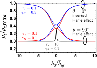
Figure 2: Spin accumulation density parallel to $\hat{z}$ in NM, under conditions of spin injection [see Fig. 1(a)], normalized to the maximum possible spin accumulation density, $p_{z,\text{max}}=\gamma_{L}\gamma_{R}\tau_{s}/A\lambda_{s}(\gamma_{R}+2\gamma_{L})$. The conventional Hanle (inverted Hanle) curves are concave down (up) and have widths sensitive (insensitive) to the spin relaxation time of traps, $\tau_{s}$. Colors (red, blue, and black) denote different $\tau_{s}$’s and $\gamma_{R}$’s chosen in the calculation. The red curves are dashed to demonstrate that the red and black parameters yield negligibly different inverted Hanle curves. $\gamma_{L}=10$ and all rates are in units of $\overline{b}_{hf}$.

ExperimentsAoki et al. (2012) on Fe/MgO/Si do observe a sharper peak of the HE superimposed upon a broader peak, as well as a broader inverted Hanle peak. The spin lifetime of the narrow peak is comparable to the one obtained in an accompanying nonlocal four-terminal experiment, which suggests an origin in direct tunneling. The presence of similarly broad peaks in the Hanle and inverted Hanle curves point to additional charge hopping through spin bottleneck sites, though contributions from hopping through spin transport sites cannot be ruled out. Other experimentsSato et al. (2015) on Fe/SiO₂/Si displayed behavior in oblique fields which suggests the importance of stray fields.

Oblique Fields.— Recently, the effect of oblique magnetic fields was measured to help distinguish spin accumulation and magnetic-field-dependent transport though barrier trapsHe et al. (2016). A strong field applied parallel to the magnetization suppresses any stray fields and returns the spin accumulation to its stray-field-free value, which for oblique fields is proportional to $\cos^{2}\theta$ for direct tunneling.Meier and Zachachrenya (1984) Ref. He et al., 2016 compared oblique measurements (solid symbols in Fig. 3) to both the direct tunneling model and the trap model (spin bottleneck sites); the result was inconclusive as both models adequately described the data.

We propose alternate quantities to distinguish the two models: the ratio of the current or spin accumulation at zero and high fields at angle $\theta$. The barrier trap model predicts a universal response whereas the stray-field model depends on the details of the magnetic layer’s roughness. Specifically,

$$i_{\text{ratio}}=\frac{\langle i(b_{0}\rightarrow\infty,\theta)\rangle-\langle i(b_{0}=0)\rangle}{\langle i(b_{0}\rightarrow\infty,\theta=0^{\circ})\rangle-\langle i(b_{0}=0)\rangle}$$ (9)

for spin extraction and

$$p_{\text{ratio}}=\frac{\langle p_{z}(b_{0}\rightarrow\infty,\theta)\rangle-\langle p_{z}(b_{0}=0)\rangle}{\langle p_{z}(b_{0}\rightarrow\infty,\theta=0^{\circ})\rangle-\langle p_{z}(b_{0}=0)\rangle}$$ (10)

for spin injection. Angular brackets denote averaging over the gaussian distribution of hyperfine fields.

In general $i_{\text{ratio}}$ can only be computed numerically but $p_{\text{ratio}}$ is analytically found to be sup

$$p_{\text{ratio}}=\frac{3\mathcal{C}(\cos^{2}\theta-1)}{2}+1$$ (11)

with

$$\mathcal{C}=\left[1-\frac{\gamma_{R}^{2}}{\overline{b}_{hf}^{2}}+\frac{\sqrt{2\pi}}{2}\frac{\gamma_{R}^{3}}{\overline{b}_{hf}^{3}}e^{{\gamma_{R}^{2}}/{2\overline{b}_{hf}^{2}}}\text{erfc}(\frac{1}{\sqrt{2}}\frac{\gamma_{R}}{\overline{b}_{hf}})\right]^{-1}$$ (12)

where, remarkably, there is no dependence on $\gamma_{L}$ nor $\tau_{s}$, and no approximations have been made on the relative size of the various rates. As shown in the Supplementsup , for either metric, if $\gamma_{R}\ll\overline{b}_{hf}\ll\gamma_{L}$ then $i_{\text{ratio}}=p_{\text{ratio}}\equiv r(\theta)=(3\cos^{2}\theta-{1})/{2}$. Figure 3 shows the oblique field data from Ref. He et al., 2016 as well as $r(\theta)$ and the agreement with the barrier trap prediction is remarkable. The fixed ratio between currents at $90^{\circ}$ and $0^{\circ}$ [$r(90^{\circ})=-1/2$] was already noted in STO/LAO/Co structuresInoue et al. (2015). Ratios near this value hold in some other experiments as well, but not allJain et al. (2012); Txoperena et al. (2013); Tinkey et al. (2014). The common occurrence of the ratio is a strong indicator that stray fields are often not the IHE mechanism. Different structures and magnets possess varying degrees of roughness and thus varying stray field distribution which have no cause to agree with $r(90^{\circ})=-1/2$.

Whether the line shapes are determined by spin transport centers or spin bottleneck centers is difficult to ascertain based solely on the angle-dependent amplitudes. The width for spin bottleneck centers, determined by the hyperfine coupling, is the same for parallel and perpendicular applied fields.sup This is not the case for spin transport centers when $\tau_{s}\overline{b}_{hf}\gg 1$; in this instance the width is governed by $\tau_{s}^{-1}$. We expect that both impurity types occur (in addition to direct tunneling) so disentangling their contributions in measurements in the literature is not feasible within the scope of this article. For $\gamma_{R}\ll\overline{b}_{hf}\ll\gamma_{L}$, both $i_{\text{ratio}}$ and $p_{\text{ratio}}$ approach $r$ but outside that strict constraint the two ratios are not identical [Fig. 3(a) vs. Fig. 3(b)]. $p_{\text{ratio}}$ is more sensitive to $\gamma_{R}$ than $i_{\text{ratio}}$.

Figure 4 summarizes the magnitudes of the conventional and pseudo HE and IHE for either spin injection (red) or spin extraction (orange). The blue curves (red dashed line) indicate slow (fast) $\gamma_{R}$ approximations for extraction (injection). Three regions are represented by red (forbidden), cyan (IHE $<$ HE), and green (IHE $>$ HE). The quantity $-x^{-1}_{\text{ratio}}(90^{\circ})$ should be interpreted as the ratio between IHE and HE: e.g. $-i^{-1}_{\text{ratio}}(90^{\circ})=\Delta i(\theta=0^{\circ})/\Delta i(\theta=90^{\circ})$

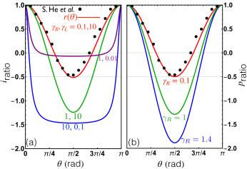
Figure 3: (a) $i_{\text{ratio}}$ and (b) $p_{\text{ratio}}$ as a function of applied field angle for a series of hopping rates (labeling each solid curve) between the spin center level and a left NM contact and right FM contact. Black circles are data from Ref. He et al., 2016. (a) Solid curves (red, purple, green, and blue) are determined from numerically averaging over the gaussian distribution of hyperfine fields for $i(0)$. (b) The results are independent of the left electrode $\rightarrow$ barrier trap hopping rate. Solid curves (black, green, and blue) are determined from Eq. (11). The red numerical line for $\gamma_{R}=0.1$, $\gamma_{L}=10$ is nearly identical to the analytic function $r(\theta)=\frac{3}{2}\cos^{2}\theta-\frac{1}{2}$.

The large-$\gamma_{R}$ asymptotic behavior of $-p^{-1}_{\text{ratio}}(\theta)$ is $2\overline{b}_{hf}^{2}\csc\theta/\gamma_{R}^{2}$ which is the dashed red line in Figure 4.

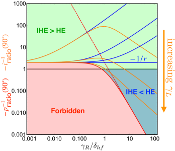
Figure 4: Ratio of the inverted Hanle effect (IHE) to the Hanle effect (HE) absolute scale factors versus $\gamma_{R}$ for either spin extraction (orange, current ratio) or spin injection (red, polarization ratio). Blue curves are for $\gamma_{R}\ll\overline{b}_{hf}$ with the horizontal blue line being $-r^{-1}(\theta)$. The dashed red line is $2\overline{b}_{hf}^{2}\csc\theta/\gamma_{R}^{2}$. Values of $\gamma_{L}$ are 0.001, 0.1, 1. As $\gamma_{L}$ increases further, the orange lines converges to the red line. $p_{\text{ratio}}$ is independent of $\gamma_{L}$

Ramifications for Non-Local Spin Detection.— For smaller voltage bias hops occur back and forth from each lead to the interfacial barrier trap. At zero bias (or zero charge current), no spin current is produced sup . Thus the described magneto-effects for spin transport centers or spin bottleneck centers cannot occur without a bias, so such effects are not expected in nonlocal measurements. Ref. Aoki et al., 2012 observes impurity-assisted signatures in three-terminal but not four-terminal devices. Thus the trap effects here will not cause confusion for spin pumping and thermal spin transport experiments involving FM/NM interfaces without charge currents. The traps as described here will not alter the spin currents without charge currents, nor can unbiased spin centers mediate ferromagnetic proximity polarization phenomenonKawakami et al. (2001); Ciuti et al. (2002); Ou et al. (2016).

Concluding Remarks. — The ambiguity in the spin-dependent magnetoresistance in a resonant tunneling formulation originates from the dependence of the Hubbard Hamiltonian ($Un_{\uparrow}n_{\downarrow}$) on the spin quantization axisSong and Dery (2014); Yue et al. (2015). Our calculations and predictions are independent of the quantization axis and agree with Ref. Song and Dery, 2014, although the reason why this is the “proper” choice is unclear; we thus suggest that the SLE approach is more robust as no assumption of an axis is required.