Carnegie Supernova Project II: The slowest rising Type Ia supernova LSQ14fmg
and clues to the origin of super-Chandrasekhar/03fg-like events

Abstract

The Type Ia supernova (SN Ia) LSQ14fmg exhibits exaggerated properties which may help to reveal the origin of the “super-Chandrasekhar” (or 03fg-like) group. The optical spectrum is typical of a 03fg-like SN Ia, but the light curves are unlike those of any SNe Ia observed. The light curves of LSQ14fmg rise extremely slowly. At $-23$ rest-frame days relative to $B$-band maximum, LSQ14fmg is already brighter than $M_{V}=-19$ mag before host extinction correction. The observed color curves show a flat evolution from the earliest observation to approximately one week after maximum. The near-infrared light curves peak brighter than $-20.5$ mag in the $J$ and $H$ bands, far more luminous than any 03fg-like SNe Ia with near-infrared observations. At one month past maximum, the optical light curves decline rapidly. The early, slow rise and flat color evolution are interpreted to result from an additional excess flux from a power source other than the radioactive decay of the synthesized ⁵⁶Ni. The excess flux matches the interaction with a typical superwind of an asymptotic giant branch (AGB) star in density structure, mass-loss rate, and duration. The rapid decline starting at around one month past $B$-band maximum may be an indication of rapid cooling by active carbon monoxide (CO) formation, which requires a low temperature and high density environment. These peculiarities point to an AGB progenitor near the end of its evolution and the core degenerate scenario as the likely explosion mechanism for LSQ14fmg.

1 Introduction

Observations of distant Type Ia supernovae (SNe Ia) led to the discovery of the accelerating expansion of the Universe (Riess et al., 1998; Perlmutter et al., 1999) and accurate measurements of the Hubble-Lemaître constant (Freedman et al., 2001). Despite the success, there is no consensus on the origin(s) of SNe Ia (e.g., Hoeflich et al., 2017; Blondin et al., 2017), beyond that they are thermonuclear explosions of carbon-oxygen white dwarfs (C/O WDs; Hoyle & Fowler, 1960). The vast majority of SNe Ia are remarkably uniform and follow the tight luminosity decline rate relation (or Phillips relation; Phillips, 1993). The bright-slow/faint-fast correlation enables SNe Ia to be used as cosmological standard candles. As observational data on SNe Ia accumulate, objects with extreme or peculiar properties have begun to emerge and form subgroups within the SN Ia classification, such as the subluminous 91bg-like (Filippenko et al., 1992a; Leibundgut et al., 1993) and 02cx-like (Li et al., 2003), as well as the overluminous 91T-like (Phillips et al., 1992; Filippenko et al., 1992b) and “super-Chandrasekhar” or 03fg-like (Howell et al., 2006) subgroups (for a review, see Taubenberger, 2017). Due to their extreme nature, the approach of identifying the origins of these subgroups which allows a clearer definition of the normal population, has been shown to be more fruitful than studying the normal objects alone (e.g., Hamuy et al., 2003; Foley et al., 2013; McCully et al., 2014; Jiang et al., 2017; De et al., 2019).

The Chandrasekhar limit (Chandrasekhar, 1931) of 1.4 $\mathrm{M}_{\odot}$ provides the theoretical mass limit above which the electron degeneracy pressure of a non-rotating WD can no longer support the star against its gravity. An exceptionally luminous SN Ia discovered by the Supernova Legacy Survey (SNLS-03D3bb or SN 2003fg; Howell et al., 2006) seemed to have defied this limit and stands out from the normal population that follows the tight Phillips relation. Subsequent discoveries of the overluminous SNe 2007if (Scalzo et al., 2010; Yuan et al., 2010) and 2009dc (Yamanaka et al., 2009; Silverman et al., 2011; Taubenberger et al., 2011) shared similar distinguishing properties and confirm this subgroup of peculiar SNe Ia, commonly referred to as “super-Chandrasekhar” SNe Ia.

As they are situated at nearly a full magnitude brighter than normal SNe Ia with similar decline rates in the Phillips relation, luminosity appeared to be the defining characteristic of this peculiar subgroup. However, the discoveries of fainter objects that share other similarities with the overluminous ones, such as SNe 2006gz (Hicken et al., 2007), 2012dn (Chakradhari et al., 2014; Parrent et al., 2016; Yamanaka et al., 2016; Taubenberger et al., 2019), and ASASSN-15pz (Chen et al., 2019) suggests a wide range of ejecta masses. As the peak luminosities of the fainter objects extend into the range of normal SNe Ia of similar decline rates, and other power sources for their luminosities are suggested (e.g., Noebauer et al., 2016), it is no longer clear that any are “super-Chandrasekhar” in ejecta mass. Thus, throughout this paper, the term “03fg-like” will be used in place of “super-Chandrasekhar,” following the convention of naming the peculiar subgroup after the first object of its kind discovered. The 03fg-like objects are extremely rare. To date, fewer than ten objects have been identified as candidates, and a few more had marginal identifying properties, such as SN 2004gu (Contreras et al., 2010), SN 2011hr (Zhang et al., 2016), LSQ12gdj (Scalzo et al., 2014), and iPTF13asv (Cao et al., 2016), pointing to possible connections to other peculiar subgroups.

The members of the 03fg-like group have relatively low decline rates in their $B$- and $V$-band light curves, positioning these SNe Ia on the bright, slowly declining end of the Phillips relation. They also have slightly longer rise times compared to normal SNe Ia. In general, the optical spectra of 03fg-like SNe Ia at maximum light resemble those of normal objects, dominated by lines of intermediate-mass elements (IMEs), such as Si, S, and Ca. However, they also show distinguishing characteristics: weak spectral lines and low expansion velocities at maximum light (as low as $8{,}000$  km s^-1 in the most luminous events). Some 03fg-like SNe Ia show evidence of substantial unburned material via strong and/or persistent optical C II features. In the near-infrared (NIR), on the other hand, the spectral features of 03fg-like and normal SNe Ia are drastically different (Hsiao et al., 2019). The prominent spectroscopic “$H$-band break” which emerges a few days after maximum light in normal objects (Kirshner et al., 1973; Elias et al., 1985; Wheeler et al., 1998) is missing or appears much later in 03fg-like objects (Taubenberger et al., 2011; Hsiao et al., 2019). Assuming that the slower rise and high luminosity result from larger amounts of ⁵⁶Ni produced, Arnett’s rule (Arnett, 1982) yields exceptionally high ⁵⁶Ni masses of $1.3-1.8$ $\mathrm{M}_{\odot}$. Even without accounting for the IMEs and unburned material observed in the spectra, some of these explosions are already near or above the Chandrasekhar mass, unless there are other energy sources at play.

A normal SN Ia with high peak luminosity and slow decline in the $B$ band typically has an $i$-band light curve that peaks before the $B$-band maximum and a prominent secondary maximum. On the other hand, all members of the 03fg-like group have late $i$-band primary maxima, occurring a few days after $B$-band maxima, and weak or no secondary maxima in the $i$ band (González-Gaitán et al., 2014; Ashall et al., 2020). The unique $i$-band morphology may be the simplest way of distinguishing members of the 03fg-like group from normal or 91T-like objects. So far, there have been only two 03fg-like objects with spectropolarimetric observations and both show very low continuum polarization similar to normal SNe Ia: ${<}0.3$% in SN 2009dc (Tanaka et al., 2010) and $0.7$% in SN 2007if (Cikota et al., 2019). For SN 2012dn, the NIR light curves were observed to have sustained high luminosities, and the excess was interpreted as an echo by circumstellar medium (Yamanaka et al., 2016). Assuming it is in an accreting WD system, the continuum polarization is predicted to be as high as 8% (Nagao et al., 2018). There are also indications that 03fg-like events are systematically overluminous in the ultraviolet compared to normal SNe Ia (Brown et al., 2014). The 03fg-like objects tend to explode in low-mass, star-forming galaxies, e.g., SNe 2003fg (Howell et al., 2006) and 2007if (Childress et al., 2011). If their host galaxies are more massive, they tend to occur in more remote locations far from the centers of their hosts, e.g., SNe 2009dc (Taubenberger et al., 2011) and 2012dn (Chakradhari et al., 2014), pointing to a preference for low metallicity or young stellar population environments.

Several theoretical explanations for the origin of the 03fg-like group have been proposed, but there is currently no single cohesive theory that explains all the observations. Differentially rotating WDs can have masses well above the Chandrasekhar limit (e.g., Durisen, 1975). However, the substantial kinetic energy required to propagate the nuclear flame is in apparent contradiction to the low photospheric velocities observed in the brightest 03fg-like events (Hachinger et al., 2012). An off-center explosion may result in nuclear burning toward a preferred direction and an asymmetric distribution of ⁵⁶Ni synthesized (e.g., Hillebrandt et al., 2007). However, these models do not reproduce the slow rise and decline in the observed light curves, but produce substantial continuum polarization and shifts in the forbidden Fe features in the nebular phase, in contradiction to observations. The merger of two WDs has also been proposed as a possible explosion scenario, either on secular (e.g., Webbink, 1984; Yoon et al., 2007) or dynamical (e.g., Pakmor et al., 2010, 2012) time scales, although an accretion induced collapse (Nomoto & Kondo, 1991) may occur rather than a thermonuclear explosion. The observed low continuum polarization also appears to disfavor off-center explosions, dynamical mergers, and even a differentially rotating WD (Uenishi et al., 2003).

The core degenerate scenario describes the merger of a WD and the degenerate core of an asymptotic giant branch (AGB) star at or shortly after the common envelope phase (e.g., Livio & Riess, 2003; Kashi & Soker, 2011). The explosion may start as a deflagration or a detonation (Hoeflich et al., 2019; Soker, 2019). This scenario should produce a spherical explosion that matches the low continuum polarization observed, but spectral interaction signatures between the ejecta and the hydrogen-rich AGB envelope have not been observed.

In this paper, we present the Carnegie Supernova Project-II (CSP-II; Phillips et al., 2019) observations of the 03fg-like SN Ia LSQ14fmg. This object exhibits several pronounced peculiar properties which are unique or best observed among the 03fg-like group and may help to reveal the origin of 03fg-like events. The data set of LSQ14fmg and possible theoretical explanations for the observed peculiarities are presented. In Section 2, details of the observations are described. In Sections 3 and 4, the photometric and spectroscopic properties of LSQ14fmg are compared to those of normal and 03fg-like SNe Ia. In Section 5, an analysis of the host galaxy of LSQ14fmg is presented. Possible theoretical explanations for the unique observed properties of LSQ14fmg are explored in Section 6, followed by a summary of conclusions in Section 7.

2 Observations

LSQ14fmg was discovered by the La Silla-QUEST Low Redshift Supernova Survey (LSQ; Baltay et al., 2013) using an image taken on 2014 September 21.03 UT and confirmed with another image taken 2 hours later. Forced photometry on pre-discovery images revealed the transient to be present as early as 2014 September 15.05 UT. The image of last non-detection was taken on 2014 August 20.21 UT, nearly one month before the first detection. The image yields a limit of $21.9\pm 0.1$ mag. Stacked images from the All-Sky Automated Survey for Supernovae (ASAS-SN; Shappee et al., 2014; Kochanek et al., 2017) provided limits at four epochs during the time gap between the last non-detection and the first detection. The Palomar Transient Factory (PTF; Law et al., 2009) and the Pan-STARRS imaging survey (Kaiser et al., 2010) did not cover the field of LSQ14fmg during the time gap. A classification spectrum was taken on 2014 September 24.95 UT with the Andalucia Faint Object Spectrograph and Camera (ALFOSC) on the Nordic Optical Telescope (NOT). LSQ14fmg was reported to be similar to a 91T-like SN Ia a few days before maximum light due to its shallow Si II features (Taddia et al., 2014).

Since the supernova redshift, determined using the classification spectrum, was well in the Hubble flow, LSQ14fmg was then followed up by CSP-II as part of the “Cosmology” sample (see Phillips et al., 2019) in the optical $BVri$ bands with the e2v CCD on the Swope Telescope and in the NIR $YJH$ bands with RetroCam on the du Pont Telescope. The photometry was computed relative to a local sequence of stars calibrated with respect to standard star fields observed over typically 20 photometric nights in the optical and three photometric nights in the NIR. The 1-$\sigma$ uncertainties presented here correspond to the sum in quadrature of the instrumental error and the nightly zero-point error. The field of LSQ14fmg was also monitored by the ESO 1-m Schmidt telescope and the Quest camera of LSQ in the broad $gr$ filter with an approximately $2$-day cadence until around maximum light. The LSQ data were reduced and the photometry was performed using the same methods as Contreras et al. (2018). The photometry is tabulated in the natural photometric system of each of Swope+e2v, du Pont+RetroCam, and LSQ+QUEST in Tables 1, 2, and 3, respectively. The color terms for transforming to the standard systems are listed in Phillips et al. (2019). Since the LSQ $gr$ band most closely resembles the $V$ band in terms of wavelength coverage, an arbitrary zero point was added to the LSQ $gr$-band light curve such that it matches the Swope $V$-band light curve. No S-corrections (Stritzinger et al., 2002) were included. All the light curves have had the host galaxy light removed using host galaxy templates taken before the explosion (LSQ) or $\sim 200$ days ($BVri$) to $\sim 300$ ($YJH$) after maximum light. These light curves are presented in Fig. 1.

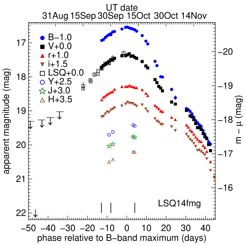
Figure 1: Optical and NIR light curves of LSQ14fmg. A non-detection limit from an image taken on 2014 August 20.21 UT by LSQ, as well as four less stringent limits from ASAS-SN, are represented by downward arrows. The short vertical lines mark the dates when the follow-up spectra were taken. The axis on the right is computed using a distance modulus of 37.26 mag. The time axis is shown in the rest-frame.

After the first classification spectrum was taken with NOT+ALFOSC, two additional follow-up spectra were also obtained with the NOT, creating a time series that spans approximately 2.5 weeks. All spectra were reduced in the standard manner using IRAF scripts. A journal of the spectroscopic observations is presented in Table 4, and the three spectra are shown in Fig. 2.

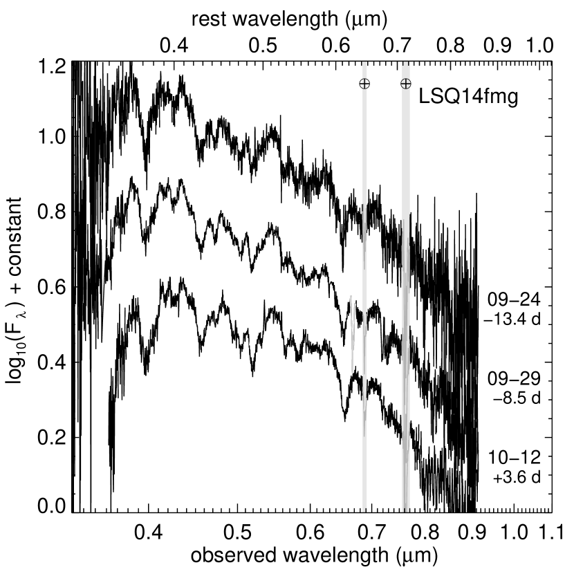
Figure 2: Optical spectra of LSQ14fmg. The UT date of the observation and rest-frame phase relative to $B$-band maximum are labeled for each spectrum. The gray vertical bands mark the regions of telluric absorptions. A sharp feature in the second spectrum near observer frame 0.67 $\mu$m is an artifact from the second-order contamination correction and is thus grayed out. There is very little spectral evolution during the $\sim 2.5$-week coverage.

The first $i$-band image taken with the Swope Telescope is shown in Fig. 3. The host galaxy of LSQ14fmg is not immediately apparent in the follow-up images. However, the site of LSQ14fmg is in the Sloan Digital Sky Survey (SDSS) Data Release 15 footprint (Aguado et al., 2019). The center of a low-luminosity galaxy, SDSS J221646.15+152114.2 coincides with the position of LSQ14fmg within 1″. We therefore assume this is the host galaxy of LSQ14fmg. After the supernova had faded, on 2015 July 19.03 UT, a spectrum of the host galaxy was taken with Wide-Field CCD (WFCCD) spectrograph on the du Pont telescope. A host galaxy heliocentric redshift of $z_{\mathrm{helio}}=0.0661\pm 0.0003$ was measured using four narrow emission lines of H$\alpha$, [N II] and [S II]. Correcting to the reference frame defined by the cosmic microwave background (CMB) radiation (Fixsen et al., 1996), the redshift becomes $z_{\mathrm{CMB}}=0.0649$. This corresponds to a distance modulus of $37.26\pm 0.03$, assuming $H_{0}=72$  km s^-1 Mpc^-1. The distance to the host galaxy of LSQ14fmg is known quite precisely due to the small uncertainty contribution from any peculiar velocities. The properties of the host galaxy are summarized in Table 5.

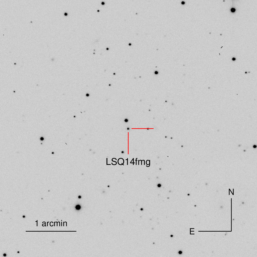
Figure 3: The first Swope $i$-band image of LSQ14fmg taken approximately two weeks before $B$ maximum. The crosshair marks the location of the supernova. The compass and the size of the field are also noted.

Integral field spectroscopy of the LSQ14fmg host galaxy was obtained on 2017 August 4, around three years after the supernova explosion, with the Multi-Unit Spectroscopic Explorer (MUSE; Bacon et al., 2010), mounted to the Unit 4 telescope (UT4) at the Very Large Telescope (VLT) of the Cerro Paranal Observatory. The observations were obtained as part of the All-weather MUse Supernova Integral-field Nearby Galaxies (AMUSING; Galbany et al., 2016) survey, aimed at studying the host environments of a large sample of nearby supernovae. The wide-field mode of MUSE provides a field-of-view of approximately 1′$\times$1′ and a squared spatial pixel of 0.2″ per side, which limits the spatial resolution. The atmospheric seeing during the observations was measured to be 1.16″. The wavelength coverage ranges from 4750 to 9300 Å, with a spectral resolution from $\lambda$/$\Delta\lambda$ $\sim$ 1800 on the blue end to 3600 on the red end of the spectrum. A detailed explanation of the data reduction is provided in Krühler et al. (2017). Briefly, version 1.2.1 of the MUSE reduction pipeline (Weilbacher et al., 2014) and the Reflex environment (Freudling et al., 2013) were used. The sky subtraction was performed using the Zurich Atmosphere Purge package (ZAP; Soto et al. 2016), employing blank sky regions within the science frame. The effects of Galactic extinction were also corrected based on the reddening estimates from Schlafly & Finkbeiner (2011). Analysis of this data is presented in Sec. 5.

Table 1: Swope+e2v photometry of LSQ14fmg in the natural system.

MJD	$B$	$V$	$r$	$i$
56925.15	17.930 (0.012)	17.736 (0.012)	17.671 (0.010)	17.677 (0.013)
56926.08	17.903 (0.008)	17.671 (0.009)	17.593 (0.008)	17.659 (0.011)
56927.10	17.843 (0.011)	17.638 (0.010)	17.559 (0.009)	17.591 (0.012)
56928.05	17.799 (0.010)	17.586 (0.008)	17.513 (0.009)	17.532 (0.010)
56929.05	17.759 (0.009)	17.544 (0.010)	17.483 (0.008)	17.544 (0.010)
56930.07	17.760 (0.032)	17.505 (0.008)	17.450 (0.008)	17.480 (0.010)
56931.10	17.679 (0.012)	17.491 (0.018)	17.431 (0.013)	17.448 (0.015)
56932.07	17.666 (0.010)	17.456 (0.009)	17.367 (0.010)	17.413 (0.012)
56936.08	17.593 (0.018)	17.381 (0.014)	17.285 (0.013)	17.355 (0.014)
56938.06	17.544 (0.025)	17.378 (0.019)	17.281 (0.019)	17.301 (0.020)
56939.07	17.537 (0.019)	17.352 (0.020)	17.284 (0.018)	17.247 (0.015)
56940.06	17.561 (0.013)	17.323 (0.016)	17.250 (0.013)	17.273 (0.013)
56941.05	17.579 (0.009)	17.396 (0.008)	17.275 (0.008)	17.278 (0.011)
56942.04	17.595 (0.008)	17.384 (0.010)	17.288 (0.009)	17.285 (0.011)
56943.03	17.616 (0.011)	17.426 (0.009)	17.311 (0.010)	17.328 (0.014)
56944.05	17.657 (0.017)	17.455 (0.017)	17.318 (0.011)	17.361 (0.015)
56947.05	17.786 (0.010)	17.549 (0.011)	17.378 (0.014)	17.326 (0.015)
56949.05	17.949 (0.010)	17.680 (0.011)	17.483 (0.009)	17.447 (0.010)
56950.05	18.033 (0.015)	17.736 (0.012)	17.549 (0.011)	17.520 (0.011)
56954.01	18.544 (0.017)	18.080 (0.012)	17.838 (0.010)	17.731 (0.013)
56955.05	18.669 (0.022)	18.170 (0.014)	17.885 (0.012)	17.803 (0.012)
56956.05	$\cdots$	18.280 (0.033)	17.937 (0.013)	17.834 (0.015)
56957.06	18.994 (0.018)	18.329 (0.014)	18.003 (0.012)	17.895 (0.014)
56958.05	19.004 (0.019)	18.411 (0.015)	18.021 (0.011)	17.903 (0.013)
56963.00	19.369 (0.054)	18.739 (0.038)	18.188 (0.025)	17.969 (0.022)
56965.03	19.613 (0.078)	18.800 (0.041)	18.254 (0.020)	18.078 (0.018)
56971.03	19.932 (0.039)	18.986 (0.031)	18.415 (0.016)	18.191 (0.016)
56972.04	19.963 (0.044)	$\cdots$	18.477 (0.014)	18.264 (0.017)
56973.03	20.017 (0.027)	19.147 (0.021)	18.565 (0.016)	18.343 (0.017)
56974.02	20.087 (0.029)	19.174 (0.020)	18.608 (0.018)	18.388 (0.017)
56975.02	20.184 (0.029)	19.259 (0.022)	18.684 (0.019)	18.455 (0.025)
56976.02	20.285 (0.042)	19.372 (0.024)	18.769 (0.020)	18.545 (0.021)
56977.02	20.347 (0.042)	19.491 (0.031)	18.832 (0.022)	18.663 (0.029)
56978.02	20.411 (0.050)	19.498 (0.028)	18.887 (0.020)	18.656 (0.017)
56979.02	20.458 (0.053)	19.545 (0.031)	18.902 (0.019)	18.701 (0.024)
56980.08	20.579 (0.055)	19.667 (0.034)	19.019 (0.020)	18.748 (0.026)
56981.03	20.690 (0.057)	19.762 (0.030)	19.079 (0.018)	18.797 (0.025)
56982.05	20.795 (0.058)	19.819 (0.031)	19.192 (0.021)	18.909 (0.023)
56983.04	20.912 (0.070)	19.991 (0.036)	$\cdots$	$\cdots$
56984.06	20.976 (0.068)	20.168 (0.048)	19.493 (0.024)	19.252 (0.030)
56986.06	$\cdots$	$\cdots$	$\cdots$	19.458 (0.134)
56994.05	$\cdots$	$\cdots$	$\cdots$	19.705 (0.100)
56996.05	$\cdots$	$\cdots$	$\cdots$	20.037 (0.132)

Table 2: du Pont+RetroCam photometry of LSQ14fmg in the natural system.

MJD	$Y$	$J$	$H$
56929.11	17.202 (0.009)	17.033 (0.012)	16.999 (0.014)
56931.16	17.119 (0.011)	16.981 (0.010)	16.932 (0.016)
56942.08	16.917 (0.010)	16.756 (0.011)	16.705 (0.015)
56942.99	16.945 (0.011)	16.781 (0.012)	16.712 (0.017)

Table 3: LSQ+QUEST photometry of LSQ14fmg in the natural system.

MJD	LSQ $gr$
56915.05	18.3453 (0.042)
56915.13	18.2650 (0.110)
56919.04	18.0967 (0.039)
56919.12	18.1374 (0.018)
56921.12	17.9322 (0.069)
56923.03	17.9187 (0.022)
56923.11	17.8252 (0.019)
56925.02	17.7274 (0.088)
56925.10	17.7614 (0.029)
56927.02	17.6167 (0.030)
56927.10	17.6105 (0.036)
56929.02	17.6052 (0.018)
56929.11	17.5840 (0.035)
56931.01	17.5045 (0.013)
56931.12	17.4551 (0.095)
56937.02	17.2903 (0.045)

Table 4: Journal of spectroscopic observations.

UT date	MJD	Instrument	$t_{\rm{max}}(B)$
2014-09-24	56924.95	NOT+ALFOSC	$-13.4$
2014-09-29	56930.10	NOT+ALFOSC	$-8.5$
2014-10-12	56943.06	NOT+ALFOSC	$+3.6$

Table 5: Properties of LSQ14fmg and its presumed host galaxy.

LSQ14fmg
$\alpha(J2000)$	334.192125°
$\delta(J2000)$	+15.353925°
$\Delta m_{15}(B)$	$1.062\pm 0.058$ mag
$s_{\mathrm{BV}}$	$1.180\pm 0.067$
JD${}_{\mathrm{max}}(B)$	$2456939.7\pm 0.5$
JD${}_{\mathrm{max}}(V)$	$2456938.5\pm 0.5$
JD${}_{\mathrm{max}}(r)$	$2456940.7\pm 0.7$
JD${}_{\mathrm{max}}(i)$	$2456940.7\pm 0.4$
$B_{\mathrm{max}}$	$17.385\pm 0.008$ mag
$V_{\mathrm{max}}$	$17.273\pm 0.008$ mag
$r_{\mathrm{max}}$	$17.175\pm 0.005$ mag
$i_{\mathrm{max}}$	$17.256\pm 0.006$ mag
$Y_{\mathrm{max}}$	$16.862\pm 0.010$ mag
$J_{\mathrm{max}}$	$16.715\pm 0.011$ mag
$H_{\mathrm{max}}$	$16.678\pm 0.015$ mag
$M_{B\mathrm{,max}}$	$-19.87\pm 0.03$ mag
$M_{V\mathrm{,max}}$	$-19.99\pm 0.03$ mag
$M_{r\mathrm{,max}}$	$-20.08\pm 0.03$ mag
$M_{i\mathrm{,max}}$	$-20.00\pm 0.03$ mag
$M_{Y\mathrm{,max}}$	$-20.40\pm 0.03$ mag
$M_{J\mathrm{,max}}$	$-20.55\pm 0.03$ mag
$M_{H\mathrm{,max}}$	$-20.58\pm 0.03$ mag
$M_{B\mathrm{,max}}$	$-20.3\pm 0.5$ mag
SDSS J221646.15+152114.2
$\alpha(J2000)$	334.192306°
$\delta(J2000)$	+15.353950°
$z_{\mathrm{helio}}$	$0.0661\pm 0.0003$
$z_{\mathrm{CMB}}$	$0.0649$
$r$	$22.40\pm 0.53$ mag
$M_{r}$	$-14.86\pm 0.53$ mag
distance modulus	$37.26\pm 0.03$ mag
E($B-V$)host	$0.13\pm 0.15$ mag
stellar mass	1.15$\pm$0.26$\times$109 M⊙
SFR	0.081$\pm$0.027 M⊙ yr-1
$\log_{10}$(sSFR[yr-1])	$-10.14\pm$0.49

3 Photometric properties

Although there is no doubt that LSQ14fmg is a SN Ia from its spectra, the light curves do not resemble those of a normal or 03fg-like SN Ia. In this section, the peculiar photometric properties of LSQ14fmg are explored.

For a peculiar and unique transient like LSQ14fmg, it is difficult to derive its host extinction from the light curves, since the intrinsic colors are unknown. A Na I D absorption feature at the host redshift is detected in the last two low-resolution spectra, which have higher signal-to-noise ratios than the classification spectrum. The equivalent widths (EWs) of the Na I D absorption of the two spectra spanning approximately two weeks are consistent with each other. Taking the value of the last spectrum, we obtained $0.82\pm 0.38$ Å. Adopting the empirical relation from Poznanski et al. (2012), while including the measurement error and the dispersion around the empirical relation (Phillips et al., 2013), yields a very uncertain color excess of E$(B-V)_{\mathrm{host}}=0.13\pm 0.16$ mag. The extinction estimate from the Balmer decrement of the MUSE observation at the location of the supernova is also consistent with zero.

Peak brightness is a key diagnostic of 03fg-like objects. The $B$-band peak apparent magnitude of LSQ14fmg without any correction is $17.385\pm 0.008$ mag. Applying $K$-corrections, Milky Way extinction correction, and the distance modulus yields an absolute magnitude of $-19.87\pm 0.03$ mag in the $B$ band. Without correcting for host extinction, the peak absolute $B$ magnitude of LSQ14fmg lies in the middle of the range for 03fg-like objects (Taubenberger, 2017). Applying the uncertain host extinction correction while assuming a total-to-selective extinction ratio of $R_{V}=3.1$, then brings the peak absolute $B$ magnitude to $-20.3\pm 0.5$ mag, one of the brightest in the 03fg-like group (Fig. 4). The photometric properties of LSQ14fmg are summarized in Table 5.

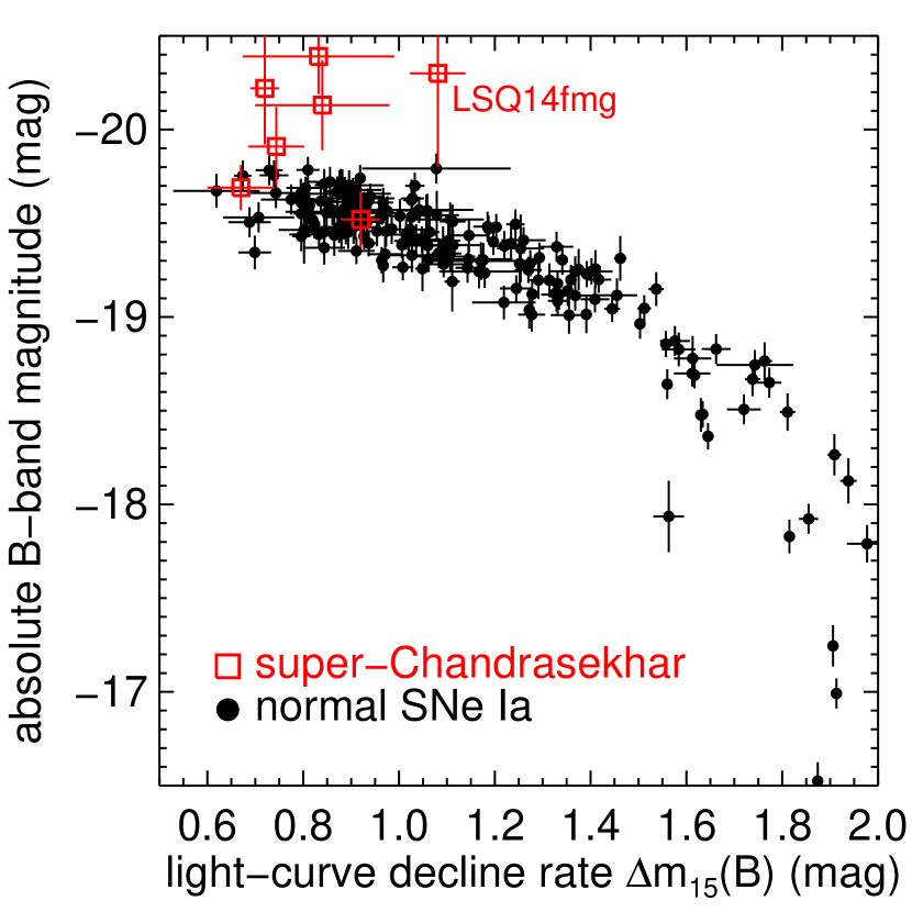
Figure 4: The Phillips relation constructed using SNe Ia observed by the CSP (Krisciunas et al., 2017; Phillips et al., 2019). Other published 03fg-like objects and LSQ14fmg in particular are highlighted for comparison.

Since there are only three observed spectra of LSQ14fmg, the time-series spectra of SN 2009dc (Silverman et al., 2011; Taubenberger et al., 2011) were used to calculate the $K$-corrections. The spectra of SN 2009dc were warped (Hsiao et al., 2007) to match the observed colors of LSQ14fmg before the $K$-corrections were computed. The uncertainty associated with this approach is measured to be less than 0.03 mag. Throughout the paper, the $B$-band maximum JD date of $2456939.7\pm 0.5$, measured using the $K$-corrected and Milky Way extinction corrected light curve, was adopted. Note that the $K$-corrected $B$-band light curve peaks slightly later than the uncorrected one published in Ashall et al. (2020), who analyzed a large sample of low-redshift peculiar objects. For other 03fg-like objects used in this paper, time-series spectra of SNe 2009dc (Silverman et al., 2011; Taubenberger et al., 2011), 2012dn (Taubenberger et al., 2019), or spectral templates of Hsiao et al. (2007) were used, depending on which data set provided the closest match to the $K$-corrections computed with observed spectra. These time-series spectroscopic data sets were chosen for their short cadence and extensive coverage in phase. For the remainder of the analysis, we use all $K$-corrected and Milky Way extinction corrected light curves, except for the LSQ+QUEST $gr$ light curve of LSQ14fmg, which is artificially shifted to match the $V$-band light curve.

In Fig. 5, the light-curve shape of LSQ14fmg is compared with a normal SN Ia and other 03fg-like objects. In the left panel, normal SN Ia SN 2012hr from the CSP-II sample (Phillips et al., 2019) was chosen since it has a very similar $\Delta m_{15}(B)$ value compared to LSQ14fmg. In the right panel, the light curves of LSQ14fmg are compared with those of SNe 2006gz (Hicken et al., 2007), 2007if (Scalzo et al., 2010; Yuan et al., 2010; Krisciunas et al., 2017), 2009dc (Taubenberger et al., 2011; Hicken et al., 2012; Krisciunas et al., 2017), 2012dn (Taubenberger et al., 2019), and ASASSN-15pz (Chen et al., 2019). All light curves are $K$-corrected except for the early LSQ $gr$ light curve of LSQ14fmg and the early ROTSE-III unfiltered light curve of SN 2007if adjusted to SDSS $r$ as described by Yuan et al. (2010). All light curves are also corrected for Milky Way extinction and time dilation. Filled symbols represent CSP data.

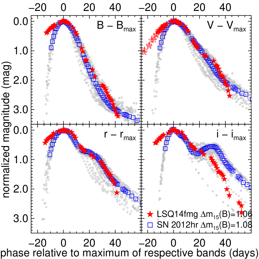
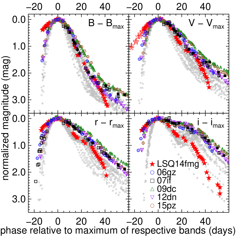
Figure 5: Light-curve shape comparisons between LSQ14fmg and a normal SN Ia with a similar decline rate (left panels) and all published low-redshift 03fg-like SNe Ia (right panels). All light curves are shifted in both the time and magnitude axes to match the peak magnitude in each band. The time axis is shown in the rest-frame of each SN Ia. SNe Ia from CSP-I and CSP-II that are well-sampled and cover extended phase range are plotted as gray circles in the background. The light curves of LSQ14fmg are plotted as filled red stars. The LSQ $gr$ light curve is plotted with the $V$ band as open red stars.

The rise of LSQ14fmg in all bands is strikingly slow compared to normal SNe Ia. The light-curve shapes of LSQ14fmg are compared with those of normal SNe Ia from CSP-I (Krisciunas et al., 2017) and CSP-II (Phillips et al., 2019) in Fig. 5. Members of the 03fg-like group have slightly longer rise times to maximum, e.g., 24 days in SN 2007if (Scalzo et al., 2010), compared to the $\sim$19-day rise time of the normal population (e.g., Conley et al., 2006). The rise time of LSQ14fmg may be much longer than any SNe Ia, and it certainly has the slowest rise ever observed in a SN Ia during the time segment from the first data point to maximum. The first light-curve point captured by LSQ is at 22.6 rest-frame days before $B$ maximum and is already as bright as $M_{V}=-19.1\pm 0.1$ mag before host extinction correction (Fig. 1). Unfortunately, the last LSQ non-detection was more than 25 days before the first LSQ point, preventing an accurate estimate of the rise time (Section 2). For an extremely bright object like SN 2009dc, the rise in the $B$ and $V$ bands is slower than most normal SNe Ia, perhaps due to a larger amount of ⁵⁶Ni produced, but is clearly still much faster than that of LSQ14fmg (right panels of Fig. 5). Early ROTSE-III data (Yuan et al., 2010) in combination with SNIFS data (Scalzo et al., 2010) in the $r$ band showed that SN 2007if, another extremely luminous 03fg-like object, also has a much faster rise than LSQ14fmg (right panels of Fig. 5). The above suggests that the extremely slow rise of LSQ14fmg is unique and the high pre-maximum luminosity may have a power source other than ⁵⁶Ni.

The post-maximum decline is not unusual in the $B$, $V$, and $r$ bands, and the decline rate lies in the slower end of this particular sample of normal SNe Ia (Fig. 5). The decline rate of LSQ14fmg as defined by Phillips (1993) is directly measured to be $\Delta m_{15}(B)$ $=1.062\pm 0.058$ mag and the color stretch parameter (Burns et al., 2014) $s_{\mathrm{BV}}$ $=1.180\pm 0.067$, which are not extreme. In the left panels of Fig. 5, the light curves of a normal SN Ia, SN 2012hr, with a similar decline rate, $\Delta m_{15}(B)$=$1.075\pm 0.009$ mag, are highlighted for comparison. The post-maximum evolution is nearly identical between SN 2012hr and LSQ14fmg in the $BVr$ bands until around one month past $B$-band maximum. The likeness to normal SNe Ia in the bluer bands, in combination with the preference for low-luminosity and star-forming hosts (Section 5), means that an object like LSQ14fmg can be a significant contaminant to a high-redshift cosmology SN Ia sample, which may only sample the bluer rest-frame bands at a few epochs. All 03fg-like SNe Ia have normal $B$-band post-maximum decline, with decline rates at the slower end of the normal SN Ia population. The differences in the post-maximum evolution between normal and 03fg-like objects become larger from blue to red filter bands (right panel of Fig. 5) as pointed out by previous studies (e.g., González-Gaitán et al., 2014).

The largest photometric differences in the optical can be seen in the $i$ band (Fig. 5). A SN Ia with high peak luminosity and relatively slow decline in the $B$ band is typically accompanied by a prominent secondary maximum in the $i$ band (e.g., Folatelli et al., 2010). In addition, the primary maximum of the $i$-band typically peaks before that of $B$ band. On the contrary, LSQ14fmg has a weak $i$-band secondary maximum and has an $i$-band primary maximum that peaks slightly after $B$-band maximum, properties which resemble that of a fast-declining, subluminous SN Ia. All members of the 03fg-like group have much weaker or no secondary maxima in the $i$ band and have the primary maxima of the $i$ band peaking after those in the $B$ band (Ashall et al., 2020). Indeed, the timing of the $i$-band primary maxima and the strength of the $i$-band secondary maxima of objects with slow-declining $B$-band light curves may be the simplest way of distinguishing members of the 03fg-like group from slow-declining normal SNe Ia or 91T-like objects. SN 2004gu was noted to be similar in peak brightness, decline rate, and spectral features to SN 2006gz by Contreras et al. (2010). However, the $iYJH$-band light curves of SN 2004gu all show strong secondary maxima. While SN 2004gu may be physically related to the 03fg-like subgroup, observationally it shares more similarities with the 91T-like subgroup. It is thus not treated as an 03fg-like event here.

Another peculiarity of LSQ14fmg surfaces at around one month past $B$-band maximum. The $B$ and $V$ light curves of normal, as well as 03fg-like SNe Ia, flatten, while those of LSQ14fmg flatten briefly around the same epoch, but then the decline rate increases rapidly around one month past maximum (Fig. 5). The unusually rapid decline is also seen to some degree in the $r$ and $i$ bands. The rapid dimming starting at around one month past maximum is a unique characteristic of LSQ14fmg even compared to the peculiar 03fg-like group. Note, however, that a few 03fg-like SNe Ia show evidence of a period of more rapid decline than normal SNe Ia, but at a much later epoch, beyond 70 days past maximum in SN 2012dn (Chakradhari et al., 2014) and beyond 200 days past maximum in SN 2009dc (Taubenberger et al., 2013; Maeda et al., 2009). Other 03fg-like may not have adequate late-time light curve coverage to characterize this dimming. This peculiar feature may be shared among 03fg-like objects and caused by a common mechanism.

The color evolution of LSQ14fmg is also unique (Fig. 6). Note that we present the observed colors, rather than attempting to obtain the intrinsic colors through the very uncertain host reddening corrections. The observed $B-V$ color shows a completely flat evolution and remains red ($B-V=0.14$) out to roughly one week past $B$ maximum. The evolution then tracks that of normal SNe Ia toward redder colors until the epoch of the Lira Law (Lira, 1996; Phillips et al., 1999) is reached. Our time coverage at this epoch is insufficient to obtain a reliable $B-V$ slope. However, the $B-V$ color tracks the blue end of the normal SN Ia sample, perhaps indicating minimal host galaxy reddening. Recall that E$(B-V)$ derived from Na I D is uncertain, but is consistent with minimal to no reddening. The observed $r-i$ color evolution of LSQ14fmg is even more remarkable. A period of flat evolution is also observed out to roughly one week past $B$ maximum and is comparatively red ($r-i=-0.11$). Furthermore, while $r-i$ curves of normal SNe Ia show the similar characteristic shape of the $B-V$ curves, the $r-i$ of LSQ14fmg is completely featureless and monotonically increasing toward redder colors with time. Other 03fg-like objects show flatter $r-i$ curves, but never as extreme.

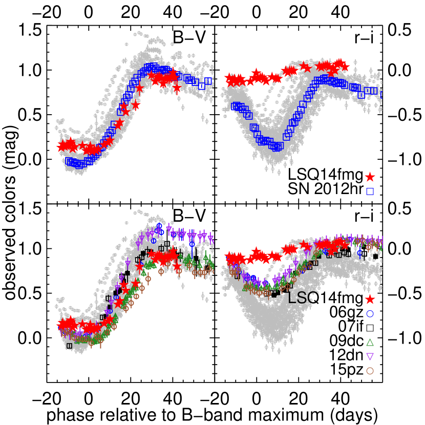
Figure 6: The observed $B-V$ (left panels) and $r-i$ (right panels) colors of LSQ14fmg. The colors are plotted in comparison to normal SNe Ia from CSP-I and CSP-II as gray backgrounds, and to SN 2012hr, a normal SN Ia of a similar $\Delta m_{15}(B)$ value (top panels), and to other 03fg-like objects (bottom panels). These plots use the same data set shown in Fig. 5 and are without host extinction corrections. The time axis is presented in the rest-frame and relative to $B$-band maximum.

LSQ14fmg is overluminous in the NIR. Our $YJH$ light curves do not have adequate time coverage for any detailed analyses. However, taking the brightest point in each band and applying only the Milky Way extinction correction and distance modulus, the $YJH$ peaks are as bright as $-20.4$ mag, $-20.6$ mag, and $-20.6$ mag, respectively. In contrast, the $YJH$ peaks for SN 2012hr, a normal SN Ia with a similar $\Delta m_{15}(B)$, are $-18.3$ mag, $-18.4$ mag, and $-18.1$ mag, respectively. LSQ14fmg is much brighter in the NIR than any normal or 03fg-like SNe Ia, including SNe 2009dc (Taubenberger et al., 2011), 2012dn (Yamanaka et al., 2016), and ASASSN-15pz (Chen et al., 2019).

4 Spectroscopic properties

Three optical spectra were taken of LSQ14fmg from approximately two weeks before to a few days past $B$ maximum. The time series spans more than two weeks, yet it shows very little evolution in the ions present and their line profile shapes (Fig. 2). The optical spectral features of LSQ14fmg are typical of 03fg-like and normal SNe Ia. Although weak, all the expected lines of IMEs are present.

In Fig. 7, the near-maximum-light spectrum of LSQ14fmg is compared to the spectra of 03fg-like SNe 2003fg (Howell et al., 2006), 2006gz (Hicken et al., 2007), 2007if (Scalzo et al., 2010), 2009dc (Taubenberger et al., 2011), 2012dn (Taubenberger et al., 2019), as well as SN 1991T (Jeffery et al., 1992), and the normal-bright SN 2011fe (Mazzali et al., 2014). Comparing the spectral features near maximum, LSQ14fmg shares many similarities with others in the 03fg-like group. The P-Cygni profiles are much weaker compared to those of normal SNe Ia, such as the well-observed, prototypical normal SN Ia SN 2011fe in Fig. 7. The pseudo-EWs of both Si II $\lambda$$\lambda$0.5972,0.6355 $\mu$m are quite small, placing LSQ14fmg solidly in the “shallow silicon” group in the Branch et al. (2006) classification scheme, along with other 03fg-like SNe Ia (Fig. 8). In fact, the Si II $\lambda$0.5972 $\mu$m line of LSQ14fmg is extremely weak in all the spectra and was difficult to identify. The measured velocity of the Si II $\lambda$0.6355 $\mu$m line is then used to locate the Si II $\lambda$0.5972 $\mu$m absorption. Indeed, LSQ14fmg has the smallest pseudo-EW of Si II $\lambda$0.5972 $\mu$m of all the members in the 03fg-like group.

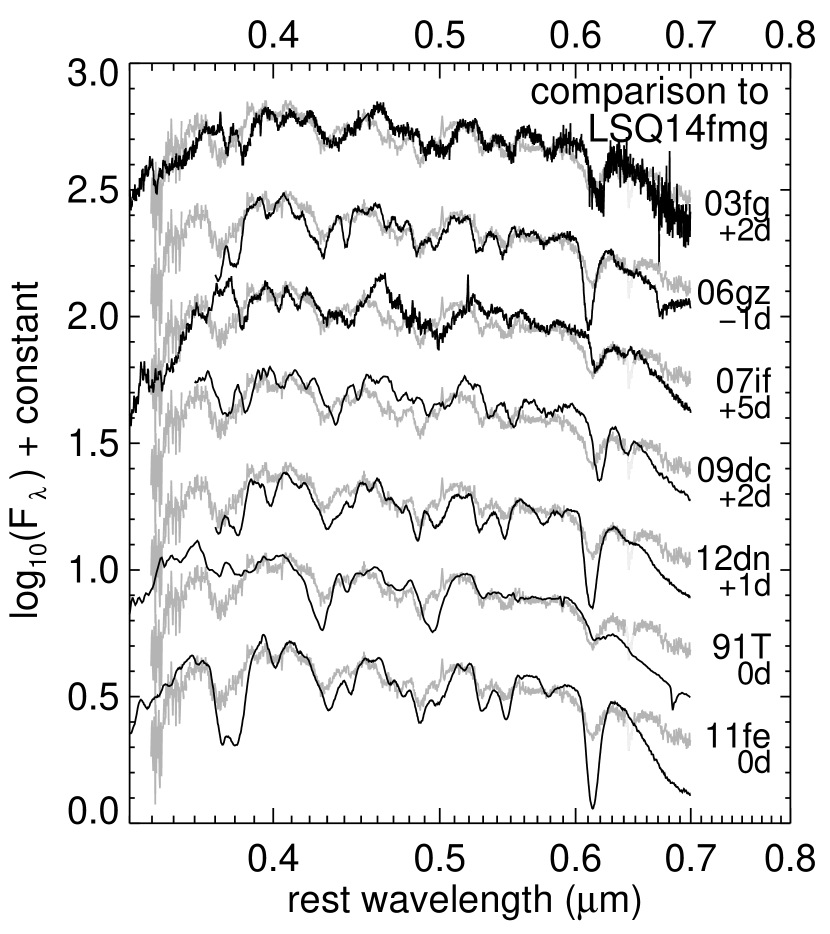
Figure 7: Comparison of near-maximum-light spectra of 03fg-like SNe Ia, SN 1991T, and the normal-bright SN 2011fe to that of LSQ14fmg. The $+3.6$ day spectrum of LSQ14fmg is plotted in the background in gray for each comparison.

Figure 8: Classification of SNe Ia based on Branch et al. (2006) into “core normal” (CN), “cool” (CL), “broad line” (BL), and “shallow silicon” (SS) subtypes. Measurements of the pseudo-EW were adopted from CSP-I (Folatelli et al., 2013). Additional measurements of the 03fg-like group were done using data from Howell et al. (2006); Hicken et al. (2007); Scalzo et al. (2010); Taubenberger et al. (2011). All members of the 03fg-like group fall in the “shallow silicon” subtype.

SYNAPPS (Thomas et al., 2011), a highly parameterized and fast spectrum synthesis code derived from SYNOW (Branch et al., 2005), identified ions which are present in normal SNe Ia in the near-maximum-light spectrum of LSQ14fmg (Fig. 9). The fit shows that the spectrum is dominated by features of IME. Carbon may be present in the spectra of LSQ14fmg. Unfortunately, both the C II $\lambda$$\lambda$0.6580,0.7235 $\mu$m lines coincide with telluric absorption lines. The presence of C II is uncertain from the SYNAPPS fit. Despite the shallow Si II lines, LSQ14fmg does not show particularly strong high-ionization Fe III lines like SN 1991T. 03fg-like SNe Ia, as a group, do not appear to be at extremely high ionization states like 91T-like objects.

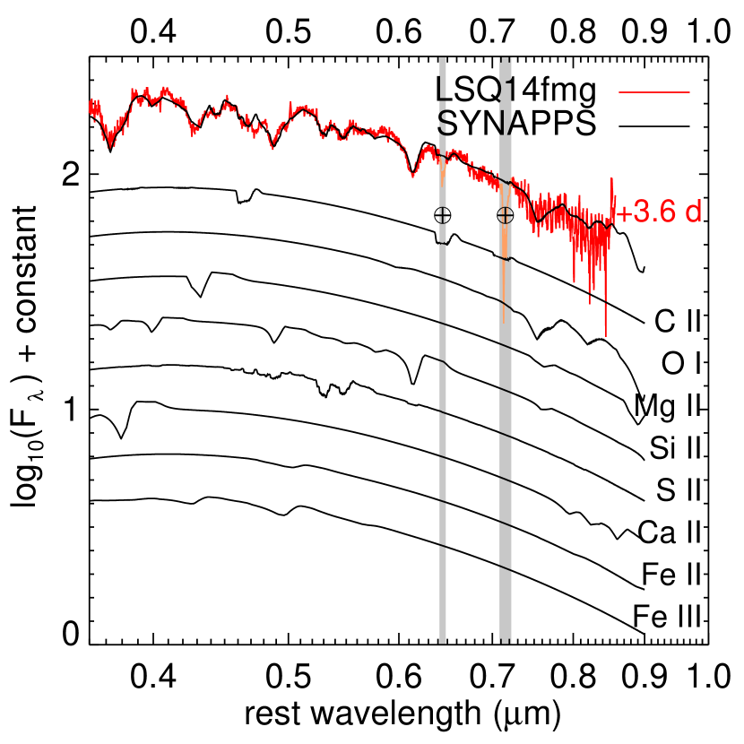
Figure 9: SYNAPPS fit of the near-maximum spectrum of LSQ14fmg. The isolated contribution of each ion is also shown. The gray vertical bands mark strong telluric absorptions, which unfortunately coincide with C II $\lambda$$\lambda$0.6580,0.7235 $\mu$m.

In Fig. 10, Si II $\lambda$0.6355 $\mu$m velocities of normal and 03fg-like SNe Ia are compared. The velocities of normal SNe Ia in CSP-I with adequate time coverage (Folatelli et al., 2013) are plotted in the background in gray, and the velocities of SNe 2009ig (Marion et al., 2013) and 2011fe (Pereira et al., 2013) are added in this group for their early-phase coverage. The shaded region represents the average and the 1$\sigma$ dispersion of the normal SN Ia sample of Folatelli et al. (2013). Velocity measurements of 03fg-like SNe Ia, SNe 2006gz (Hicken et al., 2007), 2007if (Scalzo et al., 2010), 2009dc (CSP-I), 2012dn (Taubenberger et al., 2019), and ASASSN-15pz (Chen et al., 2019) are highlighted. The Si II velocities of LSQ14fmg were measured by first removing the continuum, assumed to be a straight line connecting the blue and red boundaries of the absorption features, then fitting a Gaussian function for the minimum. To account for the uncertainty in determining the feature boundaries, velocity measurements were made on $1{,}000$ realizations of varying boundaries and random noise. The velocity errors presented include both the Gaussian fit error and the standard deviation of the realizations. Fig. 10 shows that there is a wide range of Si II velocities for the 03fg-like SNe Ia. The Si II velocity of LSQ14fmg is not in either extreme and is similar to those of the less luminous objects in the 03fg-like group, SNe 2006gz and 2012dn.

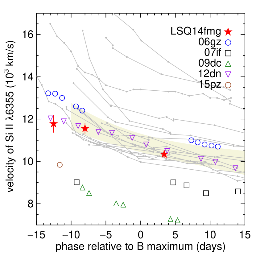
Figure 10: Comparison of the time evolution of the Si II $\lambda$0.6355 $\mu$m velocity between LSQ14fmg and other SNe Ia. The time axis is shown in the rest-frame of each SN Ia. Normal SNe Ia from CSP-I are plotted as gray in the background. The shaded region represents the average and the 1$\sigma$ dispersion of the normal sample. 03fg-like SNe Ia are highlighted.

The two earliest spectra of LSQ14fmg show Si II velocity evolving from $11{,}800\pm 400$  km s^-1 to $11{,}600\pm 200$  km s^-1, during the epoch in which Si II $\lambda$0.6355 $\mu$m of normal SNe Ia shows a rapid decline in velocity (Fig. 10). The absence of the rapid decline indicates that Si is confined at the lower-velocity range. The velocity evolution is consistent with a monotonically decreasing evolution similar to that of SN 2012dn (Taubenberger et al., 2019). From the Nearby Supernova Factory sample, Scalzo et al. (2012) identified five overluminous SNe Ia with velocity plateaus. These velocity plateaus lasted at least until 10 days past $B$ maximum. However, the ensuing drop in velocity is likely caused by the onset of Fe II features which blend with Si II $\lambda$0.6355 $\mu$m and broaden the feature toward the red, and may not represent a true decrease in the Si II velocity. The signal-to-noise ratio of our first spectrum is too low to discern whether there is a velocity plateau. Additionally, there is no evidence of the emergence of iron lines in all three spectra of LSQ14fmg. We therefore concluded that the observed decline reflects a true Si II velocity decline.

NIR spectroscopy can help reveal the physical properties of all types of supernovae (e.g. Davis et al., 2019; Hsiao et al., 2019). As shown in Fig. 6 of Hsiao et al. (2019), NIR spectroscopy can be used to easily identify a 03fg-like SN Ia. The prominent $H$-band break (Hsiao et al., 2013; Ashall et al., 2019a, b) is observed in normal SNe Ia starting a few days past maximum and results from the exposed iron-group elements (Wheeler et al., 1998). In a 03fg-like SN Ia, the $H$-band break does not appear until much later, indicating that the iron-group elements are hidden until a few months past maximum (e.g., Taubenberger et al., 2011). Unfortunately, no NIR spectra were taken of LSQ14fmg.

5 Host properties

The integral field spectroscopy obtained by MUSE was analyzed to obtain detailed host properties. First, a synthetic $r$-band image was produced by convolving the transmission of the Swope $r$-band filter with the MUSE datacube (top panel of Fig. 11). Visual inspection of the $r$-band image at the supernova position revealed an extended source which was presumed to be the host of LSQ14fmg. Based on the $r$-band brightness, a contour was defined for the extended source (Fig. 11), and the spectrum within the contour was then extracted from the datacube. The spectrum shows the typical emission lines of a star-forming galaxy on top of a blue continuum. By measuring the observed wavelengths of the strongest emission lines, the heliocentric redshift for the galaxy was determined to be $z_{\mathrm{helio}}=0.0661\pm 0.0003$, in complete agreement with the result from the WFCCD host spectrum. The $r$-band magnitude of the host was measured to be $r=22.40\pm 0.53$ from the datacube. This puts the absolute magnitude of the host galaxy at $M_{r}=-14.86\pm 0.53$.

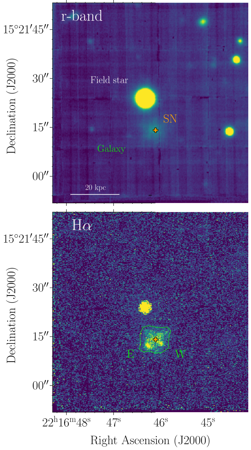
Figure 11: LSQ14fmg host galaxy images extracted from the MUSE datacube. The top panel corresponds to the synthetic $r$-band image and the bottom panel the stellar-population-subtracted and extinction-corrected gas-phase emission line map of H$\alpha$. The bright central point source is a foreground field star. The SN position is marked with a cross, and the host galaxy is defined by a green contour.

The analysis of modeling the spectrum of the host galaxy of LSQ14fmg is similar to that employed by Galbany et al. (2014, 2016), using a modified version of STARLIGHT (Cid Fernandes et al., 2005; López Fernández et al., 2016). The program models the stellar component of the observed spectral continuum by estimating the fractional contributions of simple stellar populations (SSP) of various ages and metallicities, while including the effects of foreground dust. The base model consists of 248 spectra from the “Granada-Miles” (GM) base. GM is a combination of the MILES SSP spectra (Vazdekis et al., 2010; Falcón-Barroso et al., 2011) for populations older than 63 Myr and the González Delgado et al. (2005) models for younger ages. The Initial Mass Function of Salpeter (1955) is assumed in STARLIGHT, as well as the evolutionary tracks by Girardi et al. (2000), with the exception that the youngest ages ($<$3 Myr) are based on the Geneva tracks (Schaller et al., 1992; Schaerer et al., 1993; Charbonnel et al., 1993). The GM base is defined as a regular age, metallicity $(t,Z)$ grid with 62 ages spanning $t=0.001-14$ Gyr and four metallicities ($Z/Z_{\odot}=$ 0.2, 0.4, 1, and 1.5 where $Z_{\odot}=0.02$). For the foreground dust, the Fitzpatrick (1999) reddening law with $R_{V}=3.1$ is used.

After removing the best SSP fit from each observed spectrum, a gas emission spectrum was obtained for each spaxel. The flux of the most prominent emission lines was then estimated with Gaussian fits and the dust attenuation derived from the Balmer decrement was corrected (case B recombination of Osterbrock & Ferland, 2006). From the results at each spaxel, extinction-corrected maps of the most prominent emission lines were created. For example, the extinction-corrected H$\alpha$ emission map unveils some structures on the SE and SW parts of the galaxy (the bottom panel of Fig. 11). Three spectra were then extracted from the SN location, and the SE and SW structures. The same procedures for fitting the spectra described above were applied to these three spectra to obtain the properties of the SN and host environment.

The spectra of the SN location and the SE and SW structures exhibit typical emission lines of a region with ongoing star formation, on top of a faint stellar continuum. This is confirmed by the location of their line ratios in the BPT diagram (Baldwin et al., 1981), falling below the Kewley et al. (2001) demarcation. Some environmental properties were measured for each location and are summarized in Table 6. These include the ongoing star-formation rate (SFR) as measured from the H$\alpha$ emission flux (Kennicutt, 1998), the weight of young-to-old populations from the H$\alpha$ EW, and the oxygen abundance in the O3N2 (Marino et al., 2013) and D16 (Dopita et al., 2016) scales.

Globally, a SFR of 0.081$\pm$0.027 M_⊙ yr^-1 and a stellar mass of 1.15$\pm$0.26$\times$10⁹ M_⊙ for the entire galaxy were measured, corresponding to a log of the specific SFR (sSFR) of $-10.14\pm$0.49 in yr^-1. The gas-phase metallicities are subsolar at all three locations considered as well as for the entire galaxy. The H$\alpha$ EWs are a few tens of Å, indicating a significant contribution of populations as young as $\sim$10 Myr (e.g., Kuncarayakti et al., 2018). To place the properties of LSQ14fmg’s host galaxy in the context of other SN Ia host galaxies, the sample of 215 host galaxies from the updated Pmas/Ppak Integral-field of Supernova hosts COmpilation (PISCO; Galbany et al., 2018), with properties obtained in the same fashion, was used for comparison. The host galaxy of LSQ14fmg has an extremely low stellar mass (second percentile of the PISCO host sample), similar to that of the Small Magellanic Cloud (e.g., Stanimirović et al., 2004). The SFR is low (20th percentile). However, in terms of sSFR, this low-mass galaxy is very efficient in producing new stars (90th percentile). It contains a relatively young stellar population component (80th percentile). And in both oxygen abundance calibrators, the host of LSQ14fmg ranks on the low metallicity side (10th percentile). These properties are consistent with those of other host galaxies of 03fg-like events (e.g., Childress et al., 2011).

Table 6: Properties of LSQ14fmg and host environment from the MUSE observation.

location	H$\alpha$ EW	SFR	12+$\log_{10}$(O/H)
	(Å)	(M⊙ yr-1)	O3N2 (dex)	D16 (dex)
LSQ14fmg	21.94$\pm$0.45	0.0048$\pm$0.0018	8.41$\pm$0.17	8.30$\pm$0.12
SE	37.31$\pm$0.64	0.0080$\pm$0.0016	8.34$\pm$0.17	8.20$\pm$0.12
SW	44.11$\pm$0.69	0.0045$\pm$0.0017	8.33$\pm$0.14	8.22$\pm$0.13
global	22.07$\pm$0.38	0.081$\pm$0.027	8.32$\pm$0.15	8.15$\pm$0.16

6 Discussion

Few theoretical studies have attempted to explain the 03fg-like group, partly because of the small sample size providing limited observational constraints. The peculiarities of LSQ14fmg provide insights into their origin and have guided radiation hydrodynamical simulations in order to determine the range of physical parameters governing the group and the most likely explosion scenario.

6.1 Hydrodynamical Model

Models of SN Ia explosions in a dense non-degenerate envelope had been explored by Khokhlov et al. (1993), Hoeflich & Khokhlov (1996), and more recently by Noebauer et al. (2016). They provide general explanations for several of the key observed trends in the 03fg-like group. The interaction between the ejecta and the dense envelope produces a strong reverse shock. The conversion of kinetic to luminous energy brightens and broadens the light curve, consistent with the observed slow rise and decline (Noebauer et al., 2016). This also decelerates the ejecta. Thus, more massive envelopes would, in general, manifest themselves observationally as brighter peak magnitudes and lower photospheric velocities (e.g., Quimby et al., 2007).

If we assume simply that the mass of the envelope is the only free parameter governing the 03fg-like subgroup, the inferred observational trends appear to hold for the small current sample. Within this theoretical framework, the brightest objects (e.g., SNe 2007if and 2009dc) result from explosions within the most massive envelopes and therefore have the lowest velocities (Fig. 10), slowest evolution (Fig. 5), and the most leftover unburned material (strongest C II features) compared to the faintest objects (e.g., SNe 2006gz and 2012dn). These “envelope models” are successful in reproducing some of the observables, but they do not specify the physical origin of the dense envelope. They were originally designed to mimic the WD merger scenario. However, these models are also an appropriate description for the core degenerate scenario where a WD merges with the degenerate core of an AGB star. The envelope, in this case, would be the non-degenerate envelope of the AGB star, rather than the accreted material from the secondary WD.

Given the above, we opted to compare the observations of LSQ14fmg to an updated and expanded suite of envelope models of Khokhlov et al. (1993) and Hoeflich & Khokhlov (1996) to explore the parameter space of the physical properties of the explosion. The code Hydrodynamical RAdiation (HYDRA) was used to simulate the evolution toward thermonuclear runaway and the explosion itself, as well as non-local thermodynamic equilibrium (NLTE) radiation transport to generate model light curves and spectra (Hoeflich et al., 2017, and references therein). The amount of ⁵⁶Ni produced depends on stellar evolution parameters such as main-sequence mass and metallicity, as well as when the explosion occurs (Domínguez et al., 2001). On the other hand, the envelope mass was treated as a free parameter, since the mechanisms for mass loss are not well understood.

Using the minimum Si II velocity as an indicator of the envelope mass (Quimby et al., 2007), the $10{,}000$  km s^-1 Si II velocity of LSQ14fmg (Fig. 10) corresponds to an envelope mass of roughly 0.2 $\mathrm{M}_{\odot}$. The original DET2ENV2 model of Hoeflich & Khokhlov (1996), i.e., 1.2 $\mathrm{M}_{\odot}$ degenerate core mass and 0.2 $\mathrm{M}_{\odot}$ non-degenerate envelope mass in pure detonation, has light curves too faint and narrow compared to the observations of LSQ14fmg.

Our best matching model requires a higher core mass of 1.45 $\mathrm{M}_{\odot}$, which is below the limit of $\sim 2$ $\mathrm{M}_{\odot}$ for rapidly rotating WDs (e.g., Yoon & Langer, 2005), and roughly the same envelope mass of 0.2 $\mathrm{M}_{\odot}$ as DET2ENV2. A higher mass of the degenerate core is needed to produce a sufficiently slow light curve. A star of 7 $\mathrm{M}_{\odot}$ main-sequence mass, $2\times 10^{10}$ cm radius, and metallicity Z/Z${}_{\odot}=10^{-4}$ with little H and He left in the envelope was used as a proxy for the high-mass progenitor. The model was also modified to include an initial deflagration burning phase which processed 0.2 $\mathrm{M}_{\odot}$ of material before the ensuing detonation (e.g., Poludnenko et al., 2019). The pre-expansion phase is required to avoid excessive electron capture present in classical near-Chandrasekhar-mass explosions. A prominent shell in the density structure is formed by the interaction with the non-degenerate envelope within the first few minutes of the explosion (Fig. 12). The shell then causes the confinement of materials at lower velocities, below $12{,}000$  km s^-1 (Fig. 12) which matches the observations (Fig. 10). Note that the shell is Rayleigh–Taylor unstable which may result in mixing on a scale of approximately $2{,}000$  km s^-1. The model produces ⁵⁶Ni and Si masses of 1.07 $\mathrm{M}_{\odot}$ and 0.08 $\mathrm{M}_{\odot}$, respectively, as well as small amounts of explosive C-burning products: O, Ne, Mg (Fig. 12). In general, the confinement at lower expansion velocities results in more efficient gamma-ray trapping. The results are generally high luminosities in this class of models.

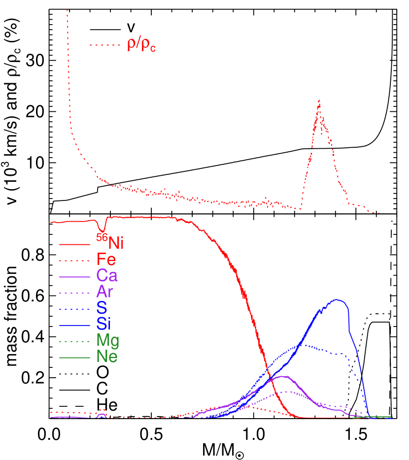
Figure 12: Density and chemical structures of the model (1.45 $\mathrm{M}_{\odot}$ degenerate core and 0.2 $\mathrm{M}_{\odot}$ envelope) that best match the observations of LSQ14fmg. The top panel plots the density structure relative to the initial central density, $\rho_{c}$, and the conversion between mass and velocity space. The bottom panel plots the chemical structure.

The comparisons between the model and observed light curves are presented in Fig. 13. The envelope model $i$-band light curve matches the observed weak secondary maximum and the overall light-curve shape, although the match is not perfect. Note that the $i$-band rise for 03fg-like objects is generally slower than those in the bluer bands (Fig. 5). The secondary maximum is formed through the expanding atmosphere in radius, and the subsequent decline coincides with the ionization transition (Hoeflich et al., 1995; Kasen, 2006). For our model, the weak secondary maximum is related to the fast receding photosphere and photospheric conditions similar to those in subluminous SNe Ia. The envelope model $B$- and $V$-band light curves suggest an early flux excess in LSQ14fmg that lasts until approximately one week after maximum and a late flux deficit that starts at approximately one month past maximum. The model spectra show stronger NIR C I lines than optical C II lines.

Figure 13: Comparison between the $B$-, $V$-, and $i$-band light curves of the envelope model (1.45 $\mathrm{M}_{\odot}$ core mass and 0.2 $\mathrm{M}_{\odot}$ envelope mass) and LSQ14fmg (red stars). Three model light curves are shown: the envelope model (thin gray curves), the same model with the effect of CO formation (dashed green curves), and with both the effects of CO formation and wind interaction (solid black curves). A W7 model light curve with 3 times the mass is plotted as gray background to represent a ⁵⁶Ni powered light curve. Note that we did not apply the uncertain host extinction correction for the analysis in this section and assumed that host extinction is negligible (Section 3).

6.2 Wind Interaction

Note that an enormous amount of ⁵⁶Ni would be required to match the extremely slow rise of LSQ14fmg. By doing so, it would result in large discrepancies in the radioactive decay tail of the light curves, . In Fig. 13, the $V$-band light curve of LSQ14fmg is compared to a simple W7 model (Nomoto et al., 1984). The mass of W7 needs to be increased by 3 times to approach the peak luminosity of LSQ14fmg. This implies a total mass of $>4$ $\mathrm{M}_{\odot}$ and pushes the IME region to as high as $42{,}000$  km s^-1, which disagrees with the observed spectra. And even then, the rising part of the model light curve is still not slow enough, hinting that an additional power source is required for the early part of the observed light curve.

Comparing the $V$-band light curves of LSQ14fmg and our envelope model described above (Fig. 13), we found a nearly constant flux difference in time from the earliest data point to approximately one week past maximum (top panel of Fig. 14). This is the same phase and duration of the flat evolution in the observed $B-V$ and $r-i$ color curves (Fig. 6). The excess flux is substantial and constitutes roughly 30% of the modeled supernova flux at peak in the $V$ band. We propose that the observed flux excess is the result of the interaction between the supernova ejecta and stellar wind. The spectral absorption features of LSQ14fmg are extremely weak even when compared with other 03fg-like events (Fig. 8); this may also be a result of the excess flux. Possible reasons for the lack of interaction signatures in the observed spectra are explored in Section 6.4.

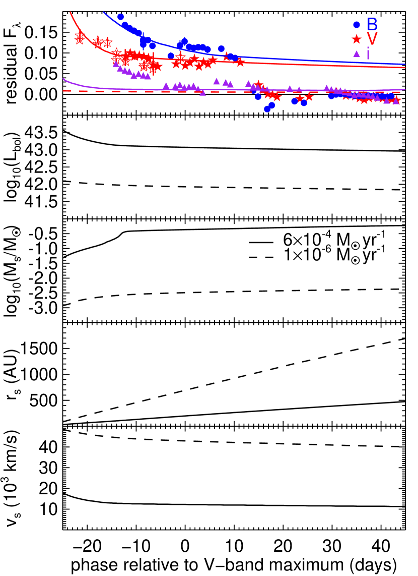
Figure 14: Wind model of the excess flux observed in LSQ14fmg. The top panel shows the model wind flux compared to the LSQ14fmg flux residual in the $B$ (blue circles), $V$ (red stars), and $i$ band (purple triangles) in ergs s^-1 cm^-2 Å^-1 while placing the model and LSQ14fmg at 10 pc. The open red stars represent LSQ $gr$ data. The remaining four panels from top to bottom illustrate the shock emission bolometric luminosity, $L_{bol}$, in $\log_{10}$ of ergs s^-1 Å^-1; shock-front mass, $M_{s}$, in $\log_{10}$ of $\mathrm{M}_{\odot}$; shock-front radius, $r_{s}$, in AU; and velocity, $v_{s}$, in  km s^-1, respectively. The mass-loss rate that matches the observed excess the best ($6\times 10^{-4}$ $\mathrm{M}_{\odot}$ yr^-1) is shown as solid curves. The mass-loss rate of $1\times 10^{-6}$ $\mathrm{M}_{\odot}$ yr^-1 is shown as dashed curves for comparison. Only the $V$-band flux for the $1\times 10^{-6}$ $\mathrm{M}_{\odot}$ yr^-1 model is shown for clarity.

We modeled the possible interaction with a stellar wind using the same approach described in Gerardy et al. (2004) but with an updated implementation. The interaction efficiently converts the kinetic energy of the rapidly expanding outer layers of the ejecta into luminosity. The impact velocity of the shock front, $v_{s}$, is well in excess of $10{,}000$  km s^-1 (Fig. 14), and the emission peaks in the hard X-ray to gamma-ray regime (0.1 to 10 MeV) and then Compton scatters. A fraction of this hard radiation will back heat the ejecta and deposit energy well below the optical photosphere, e.g., at an optical depth of $5-10$. Here, we assume that the additional energy is thermalized, and use a bolometric correction given by our explosion model to calculate the wind flux in the $B$, $V$, and $i$ band. The fact that the $B-V$ color at peak of our supernova model matches the observed $B-V$ color of LSQ14fmg, which contains the wind, supports the above assumption. The transport of hard radiation was calculated at several epochs, and we found that roughly 1/3 of the hard radiation heats the photosphere. The remaining hard radiation mostly goes into expansion work. This 1/3 factor was then used as constant in time. Momentum conservation ($\dot{M}\times v_{s}=\mathrm{constant}$) dictates that the bolometric luminosity, $L_{bol}$, starts high and declines at the beginning (Fig. 14) as the shock-front mass, $M_{s}$, piles up. Thereafter, the excess emission declines slowly because $M_{s}$ now dominates the dynamics. The time when the observed excess emission runs out (approximately one month from explosion) is used to estimate the outer edge of the wind, roughly $200-300$ AU in radius. This then places constraints on the shock-front radius, $r_{s}$, and $v_{s}$. The wind parameters which produce the best match to the observed flux excess are a wind speed of approximately 20  km s^-1 and a mass-loss rate of approximately $6\times 10^{-4}$ $\mathrm{M}_{\odot}$ yr^-1. This is slightly higher than the mass-loss rate derived from the NIR excess in SN 2012dn (Nagao et al., 2017).

The derived mass-loss rate and wind speed are akin to those of a typical AGB superwind (e.g., van Loon et al., 2003; Marshall et al., 2004), where the star ejects most of its mass toward the end stage of the AGB phase (Vassiliadis & Wood, 1993). The duration of the excess flux is observed to last roughly one month, which corresponds to the ejecta sweeping through $\sim 10^{2}$ years of wind material spanning $\sim 200$ AU in radius. This is also consistent with the duration of a superwind episode (e.g., Meixner et al., 1997) with a size that is much larger than an AGB star. If LSQ14fmg was observed in the first few days after explosion, the wind would be optically thick and a strong early emission could be present (e.g., Piro & Morozova, 2016). An encounter with a superwind later in the SN Ia evolution may be similar to the interaction signatures observed by Graham et al. (2019). Note that any pre-existing dust in the superwind is likely evaporated within days.

If the superwind interpretation is correct, it is unlikely that this is the first superwind episode of the AGB progenitor. Assuming that previous superwind episodes have the same mass-loss rate and duration as derived here, we attempt to predict some observables from the upcoming impacts here. If the density of the medium between superwind shells is zero due to reverse shocks, the ejecta of LSQ14fmg is expected to produce $3-4$ rebrightening phases due to these impacts. To estimate the X-ray and radio luminosities, Equations 51 and 52 of Dragulin & Hoeflich (2016) were used, respectively, with the same approximations. As input to the equations, the time is taken as the amount it took the superwind to reach the location of the shock interaction and the brightness temperature is derived from the mean kinetic energy of the ejecta at the time of impact. To calculate the luminosities of lower-energy photons, we assume the spectral energy distribution of the explosion model at day 100 and consider the direct emission from the shock material at 10 pc. This may stand as a proxy for the luminosity in $H_{\alpha}$, in the ultraviolet, or in $U$ and $B$ bands, depending on the abundances of the ejected material. The results are summarized in Table 7 for three upcoming rebrightening phases and for three cases where the periods of recurring superwind episodes are $5{,}000$, $10{,}000$, and $50{,}000$ years. The values are reported in the rest frame of the model. Note that the duration of the brightening phase depends on the thickness of the superwind shells and if the superwind shell becomes dispersed, the luminosities given here would be correspondingly lowered.

Table 7: Prediction of upcoming impacts with previous superwind episodes for LSQ14fmg.

period of superwind	$5{,}000$ yr			$10{,}000$ yr			$50{,}000$ yr
time of impact relative to explosion (yr)	8.3	17	26	17	34	52	82	170	260
X-ray luminosity ($\log_{10}$ of ergs/s)	43.3	43.2	43.2	43.3	43.3	43.2	43.3	43.2	43.2
specific radio luminosity ($10^{-19}$ ergs/s/Hz)	1200	440	240	430	150	83	35	13	6.9
specific low-energy flux ($10^{-2}$ ergs/cm2/s/Å)	7.7	6.4	5.5	7.5	6.6	5.9	7.7	6.4	5.5

6.3 Formation of CO

Approximately $2-3$ weeks after the end of the wind interaction phase, the $B$- and $V$-band light curves show rapid decline. This may be explained by active CO formation, facilitating a period of further rapid cooling. A HYDRA module for time-dependent CO formation via neutral and charged particle reactions (e.g., Sharp & Hoeflich, 1989; Gerardy et al., 2000) is utilized here. In Fig. 13, the effect of CO formation is shown and model light curves with and without CO formation begin to diverge roughly one month past explosion in the $B$ and $V$ bands, consistent with the observation. As noted earlier, other 03fg-like events with adequate time coverage also show a period of rapid decline in light curves, but at much later phases. It is interesting to note here that the onset of the CO formation in our envelope models is not a free parameter. 03fg-like objects with faster-expanding ejecta, such as LSQ14fmg, SNe 2006gz, and 2012dn, cool faster, facilitating earlier CO formation. On the other hand, the slower expansion rates of SNe 2007if and 2009dc make it more difficult to cool, and the onset of CO formation is expected to be much later. The high mass-loss rate of the presumed AGB progenitor of LSQ14fmg due to the recent wind episode may have sped up the CO onset as well. Fig. 15 shows the model prediction of the phase of CO onset in terms of envelope mass, and observations are plotted using the minimum Si II velocity as an indicator of the envelope mass (Quimby et al., 2007). While envelope mass is the dominant factor, note that the C/O core mass and envelope composition also affect the phase of CO onset. Future follow-up efforts may use the prediction in Fig. 15 as a rough guide to provide dense-cadence and wide-wavelength coverage at these epochs of interest. Note that we did not consider Si II velocities later than 10 days past $B$ maximum, when iron lines begin to emerge.

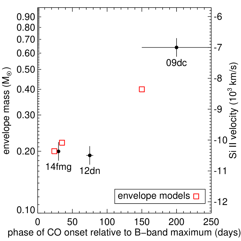
Figure 15: Model prediction of the onset of CO formation in terms of envelope mass. Observations are plotted using the minimum Si II velocity as an indicator of the envelope mass (Quimby et al., 2007). The minimum Si II velocities are taken around 5 days past maximum to avoid line blending with Fe II lines at later phases.

6.4 Core-degenerate Scenario

The observed peculiarities of LSQ14fmg all point to the progenitor being near the final stage of AGB evolution and the core degenerate scenario (e.g., Kashi & Soker, 2011) as the likely explosion mechanism. The best-matching model suggests that the progenitor has little H and He remain in the envelope. The early excess indicates the interaction with a superwind, where the AGB ejects most of its mass toward the end stage of its evolution.

The biggest weakness for the core degenerate scenario may be that no narrow emission lines, akin to those found in Type IIn SNe (Schlegel, 1990), have been observed in a 03fg-like event to indicate the interaction between the ejecta and the AGB’s envelope or wind. At least for LSQ14fmg, the indications are that its AGB progenitor is near the final phase of the evolution. Small amounts of H and He are left in the envelope, and there may not be sufficient optical depth in the wind. Furthermore, gamma-ray trapping is efficient, as is evident in the delayed onset of the $H$-band break in the NIR spectra of 03fg-like events (Taubenberger et al., 2011; Hsiao et al., 2019). Hard gamma-ray radiation from the radioactive decay of ⁵⁶Co required to excite any remaining He may have been prevented from escaping, suppressing the He I lines (e.g., Graham, 1988).

The peculiar rapid decline in the light curves of LSQ14fmg starting at around one month past $B$-band maximum indicates the onset of CO formation. CO formation requires a low temperature and high density environment. In a normal SN Ia, the expansion is too rapid for the ejecta to cool down enough to form any CO. The core degenerate scenario may have more suitable conditions for CO formation since the ejecta were cooled while enshrouded in a dense envelope. Note that the requirement for a large amount of C/O expanding at low velocities in our model is similar to that of a subluminous SN Ia, which also produces CO (Hoeflich et al., 1995). Furthermore, the copious amount of mass loss during recent episodes may have stripped most of the H and He layers, leaving a compact carbon-rich envelope. Our model then reproduces the observed early CO onset, as well as the high $i$-band and NIR luminosities caused by the efficient redistribution of flux toward the red by carbon.

In general, the low continuum polarization measured for two 03fg-like events also favors an AGB origin, since, in the WD merger scenario, a prominent thick disk is formed along with a spherical envelope (Yoon et al., 2007). Note, however, that circumstellar material farther out could produce substantial continuum polarization (Nagao et al., 2018), given the asymmetric nature of planetary nebulae. Studies of the structures of young SN Ia remnants, such as Kepler’s supernova, also indicate interaction with AGB wind (Patnaude et al., 2012) or a planetary nebula (Chiotellis et al., 2020) from the progenitor system.

Although this paper does not directly address the possible triggering mechanism, the parameters derived from the hydrodynamical simulation offer some clues. Our model infers that the degenerate core mass is high and could be above the Chandrasekhar mass but well below the limit for a rotationally supported degenerate core. An initial phase of deflagration burning is required. The deflagration phase suggests that the degenerate core may be formed by secular accretion during a common envelope phase (Hoeflich et al., 2019), rather than a merger on dynamical time scales, which would trigger a detonation. The high mass suggests that the degenerate core mass is supported by rapid rotation. The explosion may then be triggered by the contraction of the degenerate core through angular momentum transport. The high progenitor mass also disfavors dynamical merger scenarios of two massive WDs, as an accretion induced collapse is likely to result (e.g., Nomoto & Kondo, 1991).

7 Conclusions

The exaggerated light-curve properties of LSQ14fmg may help to reveal the origin of the 03fg-like group. The light curves of LSQ14fmg rise extremely slowly, even in comparison within the 03fg-like group. While the most luminous 03fg-like events have a typical rise time of $22-24$ days (Taubenberger, 2017), at $-23$ days relative to $B$ maximum, LSQ14fmg is already as bright as $M_{V}=-19.1\pm 0.1$ mag, the typical peak magnitude of a normal SN Ia (Fig. 4). The light and color curves of LSQ14fmg indicate different power sources dominating each epoch in the evolution. The $B-V$ color stays flat out to roughly one week past $B$ maximum, until SN Ia-like color curves take over. The comparison of the peculiar $V$-band light curve with an envelope model yield an apparent excess flux, indicative of interaction of the supernova ejecta with a wind-like density structure. The time-dependent flux excess suggests a mass-loss rate akin to that of a typical AGB superwind. The light curves thus have multiple power sources from the interactions with the superwind and the envelope, in addition to the radioactive decay of ⁵⁶Ni. The early peculiar rise is accompanied by a late rapid decline starting at around one month past $B$-band maximum. The rapid decline may be an indication of rapid cooling by active CO formation, which is only possible with a dense and massive C/O-rich envelope. These observations of LSQ14fmg offer three important clues about the 03fg-like group: 1) their emission is likely not entirely powered by ⁵⁶Ni; 2) the excess emission of LSQ14fmg may point to interactions with a wind that is of an AGB origin; 3) the conditions in the ejecta are favorable for CO production. All of the above point to the core degenerate scenario, the merger of a WD and the degenerate core of an AGB, as the likely explosion mechanism. Our hydrodynamical simulation suggests that LSQ14fmg explodes near the final evolutionary stage of the progenitor AGB star. A high degenerate core mass of 1.45 $\mathrm{M}_{\odot}$ and an initial deflagration phase are required to match the observations. While the core degenerate scenario provides a coherent picture of the observational properties of the 03fg-like events as a group, there are still questions left unanswered. The duration of the late AGB evolutionary phase is quite limited. Can it account for the rate of 03fg-like events? Is the explosion trigger associated with a violent mass-loss event and is the preference for low-metallicity environments associated with the mass-loss trigger? What is the relation between 03fg-like, 91T-like, and 02ic-like (Hamuy et al., 2003) events? Future observations of 03fg-like events should take into consideration predictions from the core degenerate scenario to support or refute it. These observations may also provide constraints to the uncertain mass-loss mechanisms of low-mass stars.

References

- Aguado et al. (2019) Aguado, D. S., Ahumada, R., Almeida, A., et al. 2019, ApJS, 240, 23
- Arnett (1982) Arnett, W. D. 1982, ApJ, 253, 785
- Ashall et al. (2019a) Ashall, C., Hsiao, E. Y., Hoeflich, P., et al. 2019a, ApJ, 875, L14
- Ashall et al. (2019b) Ashall, C., Hoeflich, P., Hsiao, E. Y., et al. 2019b, ApJ, 878, 86
- Ashall et al. (2020) Ashall, C., Lu, J., Burns, C., et al. 2020, ApJ, 895, L3
- Bacon et al. (2010) Bacon, R., Accardo, M., Adjali, L., et al. 2010, Proc. SPIE, 7735, 773508
- Baldwin et al. (1981) Baldwin, J. A., Phillips, M. M., & Terlevich, R. 1981, PASP, 93, 5
- Baltay et al. (2013) Baltay, C., Rabinowitz, D., Hadjiyska, E., et al. 2013, PASP, 125, 683
- Blondin et al. (2017) Blondin, S., Dessart, L., Hillier, D. J., & Khokhlov, A. M. 2017, MNRAS, 470, 157
- Branch et al. (2005) Branch, D., Baron, E., Hall, N., Melakayil, M., & Parrent, J. 2005, PASP, 117, 545
- Branch et al. (2006) Branch, D., Dang, L. C., Hall, N., et al. 2006, PASP, 118, 560
- Brown et al. (2014) Brown, P. J., Kuin, P., Scalzo, R., et al. 2014, ApJ, 787, 29
- Burns et al. (2014) Burns, C. R., Stritzinger, M., Phillips, M. M., et al. 2014, ApJ, 789, 32
- Burns et al. (2011) Burns, C. R., Stritzinger, M., Phillips, M. M., et al. 2011, AJ, 141, 19
- Cao et al. (2016) Cao, Y., Johansson, J., Nugent, P. E., et al. 2016, ApJ, 823, 147
- Chakradhari et al. (2014) Chakradhari, N. K., Sahu, D. K., Srivastav, S., & Anupama, G. C. 2014, MNRAS, 443, 1663
- Chandrasekhar (1931) Chandrasekhar, S. 1931, ApJ, 74, 81
- Charbonnel et al. (1993) Charbonnel, C., Meynet, G., Maeder, A., Schaller, G., & Schaerer, D. 1993, A&AS, 101, 415
- Chen et al. (2019) Chen, P., Dong, S., Katz, B., et al. 2019, ApJ, 880, 35
- Childress et al. (2011) Childress, M., Aldering, G., Aragon, C., et al. 2011, ApJ, 733, 3
- Chiotellis et al. (2020) Chiotellis, A., Boumis, P., & Spetsieri, Z. T. 2020, Galaxies, 8, 38
- Cid Fernandes et al. (2005) Cid Fernandes, R., Mateus, A., Sodré, L., Stasińska, G., & Gomes, J. M. 2005, MNRAS, 358, 363
- Cikota et al. (2019) Cikota, A., Patat, F., Wang, L., et al. 2019, MNRAS, 490, 578
- Conley et al. (2006) Conley, A., Howell, D. A., Howes, A., et al. 2006, AJ, 132, 1707
- Contreras et al. (2010) Contreras, C., Hamuy, M., Phillips, M. M., et al. 2010, AJ, 139, 519
- Contreras et al. (2018) Contreras, C., Phillips, M. M., Burns, C. R., et al. 2018, ApJ, 859, 24
- Davis et al. (2019) Davis, S., Hsiao, E. Y., Ashall, C., et al. 2019, ApJ, 887, 4
- De et al. (2019) De, K., Kasliwal, M. M., Polin, A., et al. 2019, ApJ, 873, L18
- Domínguez et al. (2001) Domínguez, I., Hoeflich, P., & Straniero, O. 2001, ApJ, 557, 279
- Dopita et al. (2016) Dopita, M. A., Kewley, L. J., Sutherland, R. S., & Nicholls, D. C. 2016, Ap&SS, 361, 61
- Dragulin & Hoeflich (2016) Dragulin, P., & Hoeflich, P. 2016, ApJ, 818, 26
- Durisen (1975) Durisen, R. H. 1975, ApJ, 199, 179
- Elias et al. (1985) Elias, J. H., Matthews, K., Neugebauer, G., & Persson, S. E. 1985, ApJ, 296, 379
- Falcón-Barroso et al. (2011) Falcón-Barroso, J., Sánchez-Blázquez, P., Vazdekis, A., et al. 2011, A&A, 532, A95
- Filippenko et al. (1992a) Filippenko, A. V., Richmond, M. W., Branch, D., et al. 1992a, AJ, 104, 1543
- Filippenko et al. (1992b) Filippenko, A. V., Richmond, M. W., Matheson, T., et al. 1992b, ApJ, 384, L15
- Fitzpatrick (1999) Fitzpatrick, E. L. 1999, PASP, 111, 63
- Fixsen et al. (1996) Fixsen, D. J., Cheng, E. S., Gales, J. M., et al. 1996, ApJ, 473, 576
- Folatelli et al. (2010) Folatelli, G., Phillips, M. M., Burns, C. R., et al. 2010, AJ, 139, 120
- Folatelli et al. (2013) Folatelli, G., Morrell, N., Phillips, M. M., et al. 2013, ApJ, 773, 53
- Foley et al. (2013) Foley, R. J., Challis, P. J., Chornock, R., et al. 2013, ApJ, 767, 57
- Freedman et al. (2001) Freedman, W. L., Madore, B. F., Gibson, B. K., et al. 2001, ApJ, 553, 47
- Freudling et al. (2013) Freudling, W., Romaniello, M., Bramich, D. M., et al. 2013, A&A, 559, A96
- Galbany et al. (2016) Galbany, L., Anderson, J. P., Rosales-Ortega, F. F., et al. 2016, MNRAS, 455, 4087
- Galbany et al. (2018) Galbany, L., Anderson, J. P., Sánchez, S. F., et al. 2018, ApJ, 855, 107
- Galbany et al. (2014) Galbany, L., Stanishev, V., Mourão, A. M., et al. 2014, A&A, 572, A38
- Galbany et al. (2016) Galbany, L., Stanishev, V., Mourão, A. M., et al. 2016, A&A, 591, A48
- Gerardy et al. (2000) Gerardy, C. L., Fesen, R. A., Hoeflich, P., & Wheeler, J. C. 2000, AJ, 119, 2968
- Gerardy et al. (2004) Gerardy, C. L., Hoeflich, P., Fesen, R. A., et al. 2004, ApJ, 607, 391
- Girardi et al. (2000) Girardi, L., Bressan, A., Bertelli, G., & Chiosi, C. 2000, A&AS, 141, 371
- González Delgado et al. (2005) González Delgado, R. M., Cerviño, M., Martins, L. P., Leitherer, C., & Hauschildt, P. H. 2005, MNRAS, 357, 945
- González-Gaitán et al. (2014) González-Gaitán, S., Hsiao, E. Y., Pignata, G., et al. 2014, ApJ, 795, 142
- Graham (1988) Graham, J. R. 1988, ApJ, 335, L53
- Graham et al. (2019) Graham, M. L., Harris, C. E., Nugent, P. E., et al. 2019, ApJ, 871, 62
- Hachinger et al. (2012) Hachinger, S., Mazzali, P. A., Taubenberger, S., et al. 2012, MNRAS, 427, 2057
- Hamuy et al. (2003) Hamuy, M., Phillips, M. M., Suntzeff, N. B., et al. 2003, Nature, 424, 651
- Hicken et al. (2007) Hicken, M., Garnavich, P. M., Prieto, J. L., et al. 2007, ApJ, 669, L17
- Hicken et al. (2012) Hicken, M., Challis, P., Kirshner, R. P., et al. 2012, ApJS, 200, 12
- Hillebrandt et al. (2007) Hillebrandt, W., Sim, S. A., & Röpke, F. K. 2007, A&A, 465, L17
- Hoeflich et al. (2017) Hoeflich, P., Hsiao, E. Y., Ashall, C., et al. 2017, ApJ, 846, 58
- Hoeflich & Khokhlov (1996) Hoeflich, P., & Khokhlov, A. 1996, ApJ, 457, 500
- Hoeflich et al. (1995) Hoeflich, P., Khokhlov, A. M., & Wheeler, J. C. 1995, ApJ, 444, 831
- Hoeflich et al. (2019) Hoeflich, P., Ashall, C., Fisher, A., et al. 2019, Nuclei in the Cosmos XV, held 24-29 June, 2018 in L’Aquila, Italy. Edited by A. Formicola, M. Junker, L. Gialanella, G. Imbriani. Springer Proceedings in Physics, Vol. 219, 2019, p. 187-194, 219, 187
- Howell et al. (2006) Howell, D. A., Sullivan, M., Nugent, P. E., et al. 2006, Nature, 443, 308
- Hoyle & Fowler (1960) Hoyle, F., & Fowler, W. A. 1960, ApJ, 132, 565
- Hsiao et al. (2007) Hsiao, E. Y., Conley, A., Howell, D. A., et al. 2007, ApJ, 663, 1187
- Hsiao et al. (2013) Hsiao, E. Y., Marion, G. H., Phillips, M. M., et al. 2013, ApJ, 766, 72
- Hsiao et al. (2019) Hsiao, E. Y., Phillips, M. M., Marion, G. H., et al. 2019, PASP, 131, 014002
- Jeffery et al. (1992) Jeffery, D. J., Leibundgut, B., Kirshner, R. P., et al. 1992, ApJ, 397, 304
- Jiang et al. (2017) Jiang, J.-A., Doi, M., Maeda, K., et al. 2017, Nature, 550, 80
- Kaiser et al. (2010) Kaiser, N., Burgett, W., Chambers, K., et al. 2010, Proc. SPIE, 7733, 77330E
- Kasen (2006) Kasen, D. 2006, ApJ, 649, 939
- Kashi & Soker (2011) Kashi, A., & Soker, N. 2011, MNRAS, 417, 1466
- Kennicutt (1998) Kennicutt, R. C., Jr. 1998, ApJ, 498, 541
- Kewley et al. (2001) Kewley, L. J., Dopita, M. A., Sutherland, R. S., Heisler, C. A., & Trevena, J. 2001, ApJ, 556, 121
- Khokhlov et al. (1993) Khokhlov, A., Mueller, E., & Hoeflich, P. 1993, A&A, 270, 223
- Kirshner et al. (1973) Kirshner, R. P., Willner, S. P., Becklin, E. E., Neugebauer, G., & Oke, J. B. 1973, ApJ, 180, L97
- Kochanek et al. (2017) Kochanek, C. S., Shappee, B. J., Stanek, K. Z., et al. 2017, PASP, 129, 104502
- Krühler et al. (2017) Krühler, T., Kuncarayakti, H., Schady, P., et al. 2017, A&A, 602, A85
- Krisciunas et al. (2017) Krisciunas, K., Contreras, C., Burns, C. R., et al. 2017, AJ, 154, 211
- Kuncarayakti et al. (2018) Kuncarayakti, H., Anderson, J. P., Galbany, L., et al. 2018, A&A, 613, A35
- Lantz et al. (2004) Lantz, B., Aldering, G., Antilogus, P., et al. 2004, Proc. SPIE, 5249, 146
- Law et al. (2009) Law, N. M., Kulkarni, S. R., Dekany, R. G., et al. 2009, PASP, 121, 1395
- Leibundgut et al. (1993) Leibundgut, B., Kirshner, R. P., Phillips, M. M., et al. 1993, AJ, 105, 301
- Li et al. (2003) Li, W., Filippenko, A. V., Chornock, R., et al. 2003, PASP, 115, 453
- Lira (1996) Lira, P. 1996, Masters Thesis,
- Livio & Riess (2003) Livio, M., & Riess, A. G. 2003, ApJ, 594, L93
- López Fernández et al. (2016) López Fernández, R., Cid Fernandes, R., González Delgado, R. M., et al. 2016, MNRAS, 458, 184
- Maeda et al. (2009) Maeda, K., Kawabata, K., Li, W., et al. 2009, ApJ, 690, 1745
- Marino et al. (2013) Marino, R. A., Rosales-Ortega, F. F., Sánchez, S. F., et al. 2013, A&A, 559, A114
- Marion et al. (2013) Marion, G. H., Vinko, J., Wheeler, J. C., et al. 2013, ApJ, 777, 40
- Marshall et al. (2004) Marshall, J. R., van Loon, J. T., Matsuura, M., et al. 2004, MNRAS, 355, 1348
- Mazzali et al. (2014) Mazzali, P. A., Sullivan, M., Hachinger, S., et al. 2014, MNRAS, 439, 1959
- McCully et al. (2014) McCully, C., Jha, S. W., Foley, R. J., et al. 2014, Nature, 512, 54
- Meixner et al. (1997) Meixner, M., Skinner, C. J., Graham, J. R., et al. 1997, ApJ, 482, 897
- Nagao et al. (2018) Nagao, T., Maeda, K., & Yamanaka, M. 2018, MNRAS, 476, 4806
- Nagao et al. (2017) Nagao, T., Maeda, K., & Yamanaka, M. 2017, ApJ, 835, 143
- Noebauer et al. (2016) Noebauer, U. M., Taubenberger, S., Blinnikov, S., Sorokina, E., & Hillebrandt, W. 2016, MNRAS, 463, 2972
- Nomoto et al. (1984) Nomoto, K., Thielemann, F.-K., & Yokoi, K. 1984, ApJ, 286, 644
- Nomoto & Kondo (1991) Nomoto, K., & Kondo, Y. 1991, ApJ, 367, L19
- Osterbrock & Ferland (2006) Osterbrock, D. E., & Ferland, G. J. 2006, Astrophysics of gaseous nebulae and active galactic nuclei, 2nd. ed. by D.E. Osterbrock and G.J. Ferland. Sausalito, CA: University Science Books, 2006,
- Pakmor et al. (2010) Pakmor, R., Kromer, M., Röpke, F. K., et al. 2010, Nature, 463, 61
- Pakmor et al. (2012) Pakmor, R., Kromer, M., Taubenberger, S., et al. 2012, ApJ, 747, L10
- Parrent et al. (2016) Parrent, J. T., Howell, D. A., Fesen, R. A., et al. 2016, MNRAS, 457, 3702
- Patnaude et al. (2012) Patnaude, D. J., Badenes, C., Park, S., & Laming, J. M. 2012, ApJ, 756, 6
- Pereira et al. (2013) Pereira, R., Thomas, R. C., Aldering, G., et al. 2013, A&A, 554, A27
- Perlmutter et al. (1999) Perlmutter, S., Aldering, G., Goldhaber, G., et al. 1999, ApJ, 517, 565
- Phillips (1993) Phillips, M. M. 1993, ApJ, 413, L105
- Phillips et al. (2019) Phillips, M. M., Contreras, C., Hsiao, E. Y., et al. 2019, PASP, 131, 014001
- Phillips et al. (1999) Phillips, M. M., Lira, P., Suntzeff, N. B., et al. 1999, AJ, 118, 1766
- Phillips et al. (2013) Phillips, M. M., Simon, J. D., Morrell, N., et al. 2013, ApJ, 779, 38
- Phillips et al. (1992) Phillips, M. M., Wells, L. A., Suntzeff, N. B., et al. 1992, AJ, 103, 1632
- Piro & Morozova (2016) Piro, A. L., & Morozova, V. S. 2016, ApJ, 826, 96
- Poludnenko et al. (2019) Poludnenko, A. Y., Chambers, J., Ahmed, K., Gamezo, V. N., & Taylor, B. D. 2019, Science, 366, aau7365
- Poznanski et al. (2012) Poznanski, D., Prochaska, J. X., & Bloom, J. S. 2012, MNRAS, 426, 1465
- Quimby et al. (2007) Quimby, R., Hoeflich, P., & Wheeler, J. C. 2007, ApJ, 666, 1083
- Riess et al. (1998) Riess, A. G., Filippenko, A. V., Challis, P., et al. 1998, AJ, 116, 1009
- Salpeter (1955) Salpeter, E. E. 1955, ApJ, 121, 161
- Scalzo et al. (2012) Scalzo, R., Aldering, G., Antilogus, P., et al. 2012, ApJ, 757, 12
- Scalzo et al. (2010) Scalzo, R. A., Aldering, G., Antilogus, P., et al. 2010, ApJ, 713, 1073
- Scalzo et al. (2014) Scalzo, R. A., Childress, M., Tucker, B., et al. 2014, MNRAS, 445, 30
- Schaerer et al. (1993) Schaerer, D., Meynet, G., Maeder, A., & Schaller, G. 1993, A&AS, 98, 523
- Schaller et al. (1992) Schaller, G., Schaerer, D., Meynet, G., & Maeder, A. 1992, A&AS, 96, 269
- Schlafly & Finkbeiner (2011) Schlafly, E. F., & Finkbeiner, D. P. 2011, ApJ, 737, 103
- Schlegel (1990) Schlegel, E. M. 1990, MNRAS, 244, 269
- Shappee et al. (2014) Shappee, B. J., Prieto, J. L., Grupe, D., et al. 2014, ApJ, 788, 48
- Sharp & Hoeflich (1989) Sharp, C. M., & Hoeflich, P. 1989, Highlights of Astronomy, 8, 207
- Silverman et al. (2011) Silverman, J. M., Ganeshalingam, M., Li, W., et al. 2011, MNRAS, 410, 585
- Soker (2019) Soker, N. 2019, New A Rev., 87, 101535
- Soto et al. (2016) Soto, K. T., Lilly, S. J., Bacon, R., Richard, J., & Conseil, S. 2016, MNRAS, 458, 3210
- Stanimirović et al. (2004) Stanimirović, S., Staveley-Smith, L., & Jones, P. A. 2004, ApJ, 604, 176
- Stritzinger et al. (2002) Stritzinger, M., Hamuy, M., Suntzeff, N. B., et al. 2002, AJ, 124, 2100
- Taddia et al. (2014) Taddia, F., Stritzinger, M., Hsiao, E. Y., et al. 2014, The Astronomer’s Telegram, 6495,
- Tanaka et al. (2010) Tanaka, M., Kawabata, K. S., Yamanaka, M., et al. 2010, ApJ, 714, 1209
- Taubenberger et al. (2011) Taubenberger, S., Benetti, S., Childress, M., et al. 2011, MNRAS, 412, 2735
- Taubenberger et al. (2019) Taubenberger, S., Floers, A., Vogl, C., et al. 2019, MNRAS, 488, 5473
- Taubenberger et al. (2013) Taubenberger, S., Kromer, M., Hachinger, S., et al. 2013, MNRAS, 432, 3117
- Taubenberger (2017) Taubenberger, S. 2017, Handbook of Supernovae, 317
- Thomas et al. (2011) Thomas, R. C., Nugent, P. E., & Meza, J. C. 2011, PASP, 123, 237
- Uenishi et al. (2003) Uenishi, T., Nomoto, K., & Hachisu, I. 2003, ApJ, 595, 1094
- van Loon et al. (2003) van Loon, J. T., Marshall, J. R., Matsuura, M., & Zijlstra, A. A. 2003, MNRAS, 341, 1205
- Vassiliadis & Wood (1993) Vassiliadis, E., & Wood, P. R. 1993, ApJ, 413, 641
- Vazdekis et al. (2010) Vazdekis, A., Sánchez-Blázquez, P., Falcón-Barroso, J., et al. 2010, MNRAS, 404, 1639
- Webbink (1984) Webbink, R. F. 1984, ApJ, 277, 355
- Weilbacher et al. (2014) Weilbacher, P. M., Streicher, O., Urrutia, T., et al. 2014, Astronomical Data Analysis Software and Systems XXIII, 485, 451
- Wheeler et al. (1998) Wheeler, J. C., Hoeflich, P., Harkness, R. P., & Spyromilio, J. 1998, ApJ, 496, 908
- Yamanaka et al. (2009) Yamanaka, M., Kawabata, K. S., Kinugasa, K., et al. 2009, ApJ, 707, L118
- Yamanaka et al. (2016) Yamanaka, M., Maeda, K., Tanaka, M., et al. 2016, PASJ, 68, 68
- Yoon & Langer (2005) Yoon, S.-C., & Langer, N. 2005, A&A, 435, 967
- Yoon et al. (2007) Yoon, S.-C., Podsiadlowski, P., & Rosswog, S. 2007, MNRAS, 380, 933
- Yuan et al. (2010) Yuan, F., Quimby, R. M., Wheeler, J. C., et al. 2010, ApJ, 715, 1338
- Zhang et al. (2016) Zhang, J.-J., Wang, X.-F., Sasdelli, M., et al. 2016, ApJ, 817, 114