On Thermodynamics of AdS Black Holes with Scalar Hair
Abstract
It has been known that in the presence of a scalar hair there would be a distinct additional contribution to the first law of black hole thermodynamics. While it has been checked in many examples, a deeper understanding of this issue is necessary. The thermodynamics of AdS black holes in Einstein-scalar gravity is studied by using the standard holographic renormalization procedure and the variation of the Hamiltonian via the Wald formalism. It is found that the first law requires a modification by including an additional term that has a particular form , with and a new pair of thermodynamic conjugate variables. is the leading source term of the asymptotic fall-off of the scalar field near the AdS boundary, and is precisely the response of the dual scalar operator from the holographic point of view. Some hairy black holes are constructed explicitly to check the first law of thermodynamics as well as the thermodynamic relations.
1 Introduction
The discovery of the thermodynamics of black holes has revealed a deep and fundamental relationship among gravitation, thermodynamics and quantum theory. It was achieved primarily by using classical and semiclassical analysis and has been given rise to most of our present physical understandings into the nature of quantum phenomena in the strong gravity regime [1, 2]. Over a long period in the past, it was established that black holes are uniquely specified by asymptotic charges, because of a number of black hole theorems. Nevertheless, more recently, motivations from higher dimensions, string theory and holography have led to considerations that violate many of the assumptions of these black hole theorems. Many new black hole solutions have been constructed and investigated, and the physics of black holes becomes more abundant than previously believed [3, 4]. One of the simplest and most interesting cases is black holes with a scalar field, and there are increasing number of black hole solutions with non-trivial scalar hair in the literature. Despite recent progress, the subject of scalar hair and its contribution to the first law of black hole thermodynamics remain to be elucidated.
It has been shown [5, 6] that the naively-expected first law of thermodynamics for the Einstein-scalar black holes does not hold, where is the energy or mass of a black hole, and and are the Hawking temperature and the Bekenstein-Hawking entropy, respectively. More precisely, for the (d+1)-dimensional Einstein-scalar gravity
| (1) |
the first law of AdS black holes should be modified with the full differential being shifted by a 1-form:
| (2) |
where and are two coefficients of the asymptotic fall-off of the scalar field near the AdS boundary. The first law then becomes
| (3) |
The two constants and depend on the spacetime dimension and the mass of the scalar field. In particular, it was emphasized that , and therefore the contribution in (2) is not integrable. While it has been argued that and describe the potential and charge of the scalar hair that breaks some of the asymptotic AdS symmetries [7], the physical meaning of and is unclear. 222 was considered as the scalar charge in [7], but no conserved current associated with this charge has been known so far. As the Einstein-scalar gravity is the simplest case in a variety of gravity and supergravity theories, and has wide applications in many fields, it would be of great interest to have a further understanding on the first law of black holes with non-trivial scalar hair and the physical meaning of the new pair of variables and . In particular, in many studies of holographic QCD the black holes with scalar hair were constructed to mimic QCD phenomenology in a strongly coupled regime, for which some physical observables were obtained by using the traditional first law of black holes together with some thermodynamic relations, see e.g. [8, 9, 10, 11, 12]. 333For example, the pressure or free energy is computed directly by integrating the first law of thermodynamics, while keeping all sources fixed. However, if the first law needs to be modified in the presence of the scalar hair by the form (3), one must take the new modification (2) into consideration when discussing the equation of state and other thermodynamic properties.
Although there are some discussions to deal with this issue in the literature, most of them imposed a special relationship on the coefficients and (see e.g. [13, 14, 15, 16]). In this so-called “designer gravity” the boundary conditions of the scalar in the AdS boundary are modified, such that and are independent. In some sense, it means that only a special branch of hairy black hole solutions will be considered. This raises an interesting question: Is it possible to formulate a unified version of the first law of black hole thermodynamic without imposing a special relationship on the coefficients and ? In the present paper, we investigate the thermodynamics of the AdS black holes in Einstein gravity coupled to a scalar field described by the action (1). We adopt the standard holographic renormalization procedure [17] to define thermodynamic variables, such as energy, pressure and free energy. Then we use the Wald formalism [18, 19] to derive the first law of black hole thermodynamics. We show how the scalar hair contributes non-trivially to the first law of thermodynamics. In contrast to (3), we find that the contribution from scalar hair has a particularly simple and instructive form, from which we are able to give a clear physical interpretation for both and . We also construct the hairy black holes explicitly to demonstrate their existence and to numerically check the resulting thermodynamic relations. Finally, a general argument is given for the form of scalar hair contribution to the first law of thermodynamics.
2 Setup and Background
We are interested in the thermodynamics of the (d+1)-dimensional asymptotically AdS black holes in Einstein-scalar theory (1). We consider the planar black holes with the ansatz given by
| (4) |
for which the location of the event horizon is at where . We take the geometry at the black hole boundary to be . Although we focus on the case with planar symmetry in the present study, our discussion below should apply to black holes with spherical and hyperbolic horizon geometries.
Near the AdS boundary, one has , with the AdS curvature scale, and . 444In general one only needs to approach a constant near the AdS boundary. But it should not be thought of as a free parameter, as it can be absorbed into a rescaling of the time coordinate. We choose such that the asymptotic AdS metric has a canonically normalized time coordinate, i.e. we are interested in the boundary system with respect to the metric . Without loss of generality, near the AdS boundary we parameterize the scalar potential as follows
| (5) |
where we have chosen at the black hole boundary for convenience, and the parameter is the mass of the scalar field. Then the asymptotic expansion for the scalar near the AdS boundary is schematically given by
| (6) |
where , and and are two constants. In order to allow the most general solutions with two non-trivial parameters and , we have considered the case where the mass-squared of the scalar field is negative, but above the Breitenlohner-Freedman (BF) bound , i.e. . 555There is a special case saturating the BF bound with , for which the scalar asymptotics behaves different from (6). This case does not change our discussion below and a concrete example is presented in the appendix. Following the spirit of holography, we call the leading term as the source. 666For the mass range slightly above the BF bound, , the two falloffs of (6) are both normalizable and either one can be considered as a source, corresponding to two different dual field theories [20]. We will only consider standard quantization for the scalar field throughout the manuscript. In the rest of our discussion, without loss of generality, we shall work with for simplicity by fixing in such a way the length unit.
The equations of motion that follow from the action (1) are:
| (7) |
| (8) |
Substituting the ansatz (4) into the above equations of motion, we obtain the following equations of motion:
| (9) |
where only two of the last three equations are independent. The temperature and entropy density associated with the above background are given by
| (10) |
respectively.
Making use of (9), we can obtain a radial conserved quantity 777For black holes with spherical and hyperbolic horizon topologies, there is an extra term in due to non-vanishing curvature of horizons [21].
| (11) |
which connects horizon to boundary data. Evaluating (11) at the horizon and using (10), one finds
| (12) |
Therefore, signals extremity. As a consequence, for the Einstein-scalar theory the extremality condition implies is a constant, and thus extremal geometries are relativistic independently of which potential one chooses [22]. The extremal geometry is described by a metric of the form
| (13) |
where for convenience we have set . In order to compute at the AdS boundary , one needs to know the boundary asymptotics for the bulk fields and , which depend on the details of the theory one considers.
3 Wald Formula
Our next step is to consider the first law of thermodynamics for our Einstein-scalar black holes (4). We will adopt the general procedure developed by Wald [18]. In Wald’s procedure, one considers the variation of the parameters in a (d+1) dimensional solution, and constructs a closed (d-1)-form with a Killing vector. To make contact with the first law of black hole thermodynamics, we take , i.e. the time-like Killing vector that is null on the horizon. Then one introduces the integral
| (14) |
over any (d-1)-dimensional surface at constant and . It has been shown by [18] that the variation of the Hamiltonian is independent of .
For our present case (4) of the Einstein-scalar theory, we follow the derivation presented in [5, 6] and obtain that
| (15) |
Then at radius is given by
| (16) |
with the spatial volume of the (d-1)-plane. Since is a radially conserved quantity, it can be evaluated at any position. Near the horizon at , we have
| (17) |
Thus , and we obtain
| (18) |
where we have used .
In order to evaluate (16) at the boundary, one should know the boundary asymptotics for three bulk fields , and . The expansions near the black hole boundary depend on the precise form of . For a given potential , one can in principle obtain the full asymptotic form by taking appropriate large- expansions for , and , inserting them into the equations of motion (9), and solving for the coefficients in the expansions up to some desired order. In practice, it is in general difficult to make the appropriate expansions due to the backreaction of the scalar to the metric. In certain cases, there is logarithmic dependence in the asymptotic expansions for the metric and scalar fields.
Furthermore, we also need to obtain the mass of the Einstein-scalar black holes, for which we use the standard holographic techniques. More precisely, we calculate the renormalized stress tensor for the dual boundary theory and the mass is obtained from the component of the holographic stress tensor, i.e. . In order to do that, we should add appropriate boundary terms and counterterms to the bulk action to remove divergences in the holographic stress tensor, which also depends on the non-linear detail of the coupling . To avoid above complications, our strategy is to consider some representative “benchmark” models in this work. We will find the precise form of boundary asymptotics and will examine the thermodynamics of the black hole solutions via the holographic renormalization.
4 Five Dimensional Case
For the five-dimensional case, we consider the following class of potentials:
| (19) |
with a constant. Near the AdS boundary where , one has
| (20) |
Therefore, the the cosmological constant is given by with the AdS radius and of (6).
Using the equations of motion (9), the boundary asymptotics as for the bulk fields and are found to be
| (21) |
We point out that due to the non-trivial source , there are terms with dependence in the above expansion. As we have pointed out, we will set to fix the normalization of time.
4.1 Thermodynamic relation
To read off the physical observables via the holographic renormalization, we need to consider appropriate boundary terms in the UV. For the present class of models with given in (19), the boundary terms are found to be
| (22) |
where is the induced metric at the AdS boundary and the extrinsic curvature defined by the outward pointing normal vector to the boundary between . The first term of (22) is Gibbons-Hawking term for a well-defined Dirichlet variational principle, and the three local covariant surface counterterms in the middle are required to remove divergences. The last term is a finite counterterm with typically a constant free parameter, which defines a renormalization scheme. As will be demonstrated below, most of the thermodynamic variables depend on the parameter . Note also that the coefficient of the logarithmic term depends on the model parameter . According to the holographic dictionary, the holographic stress tensor is
| (23) |
and the condensate for the dual scalar operator reads
| (24) |
Inserting the boundary expansions of the bulk fields (21) into (23), we obtain the non-vanishing components of the stress tensor
| (25) |
where is the pressure and is the energy density which is also known as the mass density of the black hole. 888In our discussion the boundary geometry possesses a time-like Killing vector . We define the energy density of the dual field theory as , which is equal to the energy density of the black hole via the AdS/CFT correspondence. Instead of energy and entropy of (3), we use energy density and entropy density in the planar black hole case (4). The trace of the stress tensor is given by
| (26) |
Note that there is a trace anomaly in the presence of the source term which breaks the conformal symmetry. The expectation value of the dual scalar operator obtained from (24) reads
| (27) |
It is clear that , and depend on the parameter of (22), corresponding to the renormalization scheme.
We now compute the free energy density which is identified as the temperature times the renormalized action in Euclidean signature. Since we consider a stationary problem, the Euclidean action is related to the Minkowski one by a minus sign. Therefore, we have
| (28) |
with the spatial volume and . Employing the equations of motion, we find
| (29) |
Substituting the asymptotical expansion (21) into above expression, we obtain the free energy
| (30) |
One immediately finds that the pressure reappears in the analysis as just minus the free energy, i.e. , which is expected from thermodynamics. Furthermore, evaluating the conserved quantity (11) at the AdS boundary, one obtains
| (31) |
where we have used (25). So we manage to obtain the expected thermodynamic relation
| (32) |
for the class of potentials in (19), independent of the renormalization scheme one chooses.
4.2 First law of thermodynamics
We now consider the first law of thermodynamics for our Einstein-scalar black hole by considering the Wald formula. In the present case with , we compute the radial conserved quantity
| (33) |
both at the horizon and the AdS boundary.
As we have already shown in (18), the horizon computation yields
| (34) |
Substituting the UV expansion (21) into (33) and evaluating it at infinity, we obtain
| (35) |
where the expressions for energy density (25) and condensate (27) have been used in the second and third equalities, respectively. Therefore, we have the following first law of thermodynamics
| (36) |
and in terms of free energy (32) we have
| (37) |
Although the boundary behaviors of bulk fields are sensitive to the model parameter and the thermodynamic quantities, such as and , depend on the choice of parameter in the boundary counterterms, the first law of thermodynamics can be written as above simple and compact form.
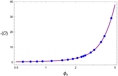
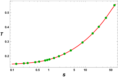
To check the first law of thermodynamics, we construct the hairy black holes by solving the equations of motion (9) numerically for the potentials (19) with . We can then read off from the black hole boundary (21), and obtain from the horizon data via (10). The presence of logarithmic terms in (21) poses some technical complications on extracting physical data. In practice, we fit the numerical solutions close to the AdS boundary using ultraviolet asymptotics (21) and obtain which are required to calculate most of the physical quantities. According to the first law (36), one should have with the entropy density fixed and with the source fixed. In figure 1, we compare and extracted from the boundary data and the first law of thermodynamics (36). The results from both ways match with each other perfectly. We also check the thermodynamic relation (32), which is found to be satisfied with high numerical accuracy.
5 Four Dimensional Case
In this section we consider a family of models in four dimensions. The potential reads
| (38) |
with a free parameter.999This particular form of scalar potential was introduced in [23]. It allows the near boundary expansion that is consistent without the logarithmic terms. Near the AdS boundary where , one has
| (39) |
from which one obtains the cosmological constant and the parameter of (6). The asymptotics for the three bulk fields and near the AdS boundary are given by
| (40) |
where we have set to fix the normalization of time. In contrast to the five dimensional case, there are no logarithmic terms in above expansions due to the particular form of potential in (38).
5.1 Thermodynamic relation
Following the holographic renormalization procedure, we introduce the counterterm action for the class of potentials (38)
| (41) |
where the first one is Gibbons-Hawking boundary term for a well-defined Dirichlet variational principle and the following two terms for removing divergence. The last term of (41) is a finite counterterm with a constant, corresponding to the freedom to choose the counterterms in holographic renormalization. Then we obtain the holographic stress tensor
| (42) |
and the condensate for the dual scalar operator reads
| (43) |
By substituting the expansions (40) into (42), we obtain the stress tensor
| (44) |
where is the pressure and is the energy (mass) density. Due to the presence of the source term , the stress tensor also has a non-vanishing trace
| (45) |
The expectation value of the dual scalar operator obtained from (43) reads
| (46) |
5.2 First law of thermodynamics
We now consider the first law of thermodynamics by using the Wald formula developed in Section 3. For the present case with , we compute the radial conserved quantity (16) at the AdS boundary and obtain that
| (50) |
Note that the variation of the energy density is given from (44) that
| (51) |
Then we find
| (52) |
where the last equation is obtained by using the expression for the condensate (46). Therefore, we have the following first law of thermodynamics
| (53) |
and in terms of free energy we have
| (54) |
Although and depend on the parameter in the boundary counterterms (38), the final form of the first law of thermodynamics is independent of .
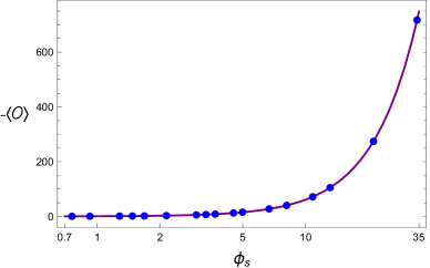
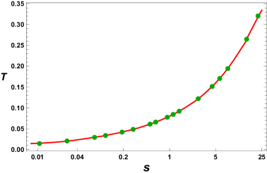
In order to further check our discussion, we construct the four dimensional hairy black holes numerically for the potentials (38), and read off thermodynamic quantities from boundary data via (10), (44) and (46). The thermodynamic relation (49) is found to be satisfied with very high numerical accuracy. In figure 2 we show the observables extracted from the first law of thermodynamics (53), including (left panel) and (right panel). Both exactly agree with the ones obtained from boundary data directly.
6 Discussion
We have examined the thermodynamics for black holes with non-trivial scalar hair in Einstein gravity coupled to a scalar field in asymptotically AdS spacetime. We defined the energy or mass of the hairy black hole from the holographic stress tensor via the standard holographic renormalization. Although the explicit expressions for thermodynamic variables, such as and , depend on the details of a model one considers, we have shown that the thermodynamic relation and the first law of thermodynamics can be written as the model-independent language already advocated in terms of thermodynamic quantities, see e.g. (32) and (36). More precisely, by incorporating the Wald formalism, we have found that the first law of thermodynamics is modified with a novel contribution from the scalar hair. One recovers the traditional first law of thermodynamics by restricting on the family of solutions with the source fixed, i.e. . We have checked numerically the new form of first law and thermodynamic relations for two families of models in five and four dimensions. 101010Although a scalar is the simplest field in any field theory, it is still difficult to obtain analytic scalar black hole solutions with general coefficients and of (6). There have been some analytic hairy black holes, see e.g. [24, 25, 26, 27, 28], but these are very special solutions for which the first law of thermodynamics does not contain any contribution from the scalar hair. The special case that saturates the BF bound was also examined in the appendix.
The new form of the first law of thermodynamics (36) seems quite natural from the holographic point of view. Identifying the leading term of the scalar in the boundary expansion (6) as the source, we introduce its conjugate using the GKPW formula [29, 30]
| (55) |
On the other hand, for a stationary background geometry, the renormalized on-shell action is closely related to the free energy via (28). Therefore, we immediately obtain
| (56) |
where we have used in the last equality. Thus, it is reasonable to consider and as a pair of thermodynamic conjugate variables in the first law.
It has been known that in the presence of a scalar hair there should be a non-trivial contribution to the first law of thermodynamics (2). While this result has been checked in many examples [5, 6, 7], a deeper and broader physical understanding is needed for this new correction. Using the standard holographic dictionary, our analysis suggests that such contribution has a particular form where is the conjugate of in terms of the renormalized on-shell action and is precisely the response of the dual operator in the presence of the source . Comparing our result with (3), we can give a clear physical interpretation on the pair of thermodynamic variables : is the source term of the scalar hair and the response of the scalar from the holographic point of view. In particular, for the branch of solutions with the source fixed, which is the typical situation for holographic applications, such additional contribution to the first law vanishes. It also means that only for the branch of black hole solutions with fixed can one obtain the pressure by directly integrating the first law of thermodynamics, i.e. .
We point out that there is some subtlety on the definition of mass for asymptotically AdS black holes. In the present work we have defined the mass using standard holographic techniques. Apart from the holographic mass, other definitions include ADM mass [31, 32], Komar mass [33, 34], Hamiltonian mass [7, 35] and so on. A thorough study on the role of different definitions of mass in the first law of thermodynamics is interesting but beyond the scope of this manuscript. Although we did not consider all possible models, our discussion suffices to illustrate the key feature we uncover. It should be helpful to examine other cases of potential with a different scalar mass. In the present study we focused on the neutral case, but our discussion can be easily extended to the charged case by adding a U(1) gauge field. It would also apply to other kinds of matter content, such as massive vector and p-from fields, by incorporating the Wald formalism and the holographic renormalization. 111111Another possible way to obtain the first law of thermodynamics is through a Hamilton-Jacobi-like analysis as discussed in [36], after considering the holographic renormalization. While we have demonstrated the first law of thermodynamic for homogeneous black holes, it will be interesting to consider black holes that break translational invariance, in particular, for the case with an inhomogeneous background geometry.
Acknowledgements
I am grateful to Rong-Gen Cai, Qiang Wen, Song He and Hong Lü for helpful discussions and comments on the manuscript. This work was supported in part by the National Key Research and Development Program of China Grant No.2020YFC2201501 and by the National Natural Science Foundation of China Grants No.12075298, No.11991052 and No.12047503.
Appendix A Scalar Mass Saturating the BF Bound
There is a special case for which the scalar mass saturates the BF bound. It is interesting and necessary to check if our discussion about the first law of thermodynamics is valid for this particular situation. As a concrete example, we consider the potential that appears in gauged supergravity in five dimensions [37]:
| (57) |
Near the AdS boundary where , one has
| (58) |
which corresponds to the cosmological constant and the scalar mass .
The boundary asymptotics as for the bulk fields and are given by
| (59) |
Note that there are complicated logarithmic terms in the presence of non-trivial source . We will set to fix the normalization of time.
To obtain the physical observables via the holographic renormalization procedure, we need to add appropriate boundary terms at the AdS boundary. For the potential in (57), the boundary terms are given by
| (60) |
where is a free parameter which defines a renormalization scheme. Then we obtain the holographic stress tensor
| (61) |
and the condensate for the scalar operator
| (62) |
Inserting the boundary expansions (59) into (61), we obtain the energy density and the pressure
| (63) |
The expectation value of the dual scalar operator obtained from (62) reads
| (64) |
Employing the equations of motion (9) and using the asymptotical expansion (59), we obtain the free energy
| (65) |
Evaluating the conserved quantity (11) at the AdS boundary, we can obtain
| (66) |
So we manage to obtain the expected thermodynamic relation
| (67) |
We now consider the first law of thermodynamics for the potential (57). As we have already shown, the horizon computation gives
| (68) |
while evaluating at infinity yields
| (69) |
where we have used the expressions (63) and (64). Therefore, we have the same form of the first law of thermodynamics
| (70) |
even for the scalar mass that saturates the BF bound. Note that the thermodynamic variables, such as and , depend on the parameter appearing in the boundary counterterms, the first law of thermodynamics has the same universal form.
References
- [1] S. F. Ross, “Black hole thermodynamics,” [arXiv:hep-th/0502195 [hep-th]].
- [2] R. M. Wald, “The thermodynamics of black holes,” Living Rev. Rel. 4, 6 (2001) [arXiv:gr-qc/9912119 [gr-qc]].
- [3] Ó. J. C. Dias, J. E. Santos and B. Way, “Numerical Methods for Finding Stationary Gravitational Solutions,” Class. Quant. Grav. 33, no.13, 133001 (2016) [arXiv:1510.02804 [hep-th]].
- [4] P. M. Chesler and L. G. Yaffe, “Numerical solution of gravitational dynamics in asymptotically anti-de Sitter spacetimes,” JHEP 07, 086 (2014) [arXiv:1309.1439 [hep-th]].
- [5] H. S. Liu and H. Lü, “Scalar Charges in Asymptotic AdS Geometries,” Phys. Lett. B 730, 267-270 (2014) [arXiv:1401.0010 [hep-th]].
- [6] H. Lü, C. N. Pope and Q. Wen, “Thermodynamics of AdS Black Holes in Einstein-Scalar Gravity,” JHEP 03, 165 (2015) [arXiv:1408.1514 [hep-th]].
- [7] H. Lü, Y. Pang and C. N. Pope, “AdS Dyonic Black Hole and its Thermodynamics,” JHEP 11, 033 (2013) [arXiv:1307.6243 [hep-th]].
- [8] S. S. Gubser and A. Nellore, “Mimicking the QCD equation of state with a dual black hole,” Phys. Rev. D 78, 086007 (2008) [arXiv:0804.0434 [hep-th]].
- [9] D. Li, S. He, M. Huang and Q. S. Yan, “Thermodynamics of deformed AdS5 model with a positive/negative quadratic correction in graviton-dilaton system,” JHEP 09, 041 (2011) [arXiv:1103.5389 [hep-th]].
- [10] S. He, S. Y. Wu, Y. Yang and P. H. Yuan, “Phase Structure in a Dynamical Soft-Wall Holographic QCD Model,” JHEP 04, 093 (2013) [arXiv:1301.0385 [hep-th]].
- [11] R. Rougemont, A. Ficnar, S. Finazzo and J. Noronha, “Energy loss, equilibration, and thermodynamics of a baryon rich strongly coupled quark-gluon plasma,” JHEP 04, 102 (2016) [arXiv:1507.06556 [hep-th]].
- [12] Z. Fang and Y. L. Wu, “Equation of state and chiral transition in soft-wall AdS/QCD with more realistic gravitational background,” [arXiv:1909.06917 [hep-ph]].
- [13] T. Hertog and G. T. Horowitz, “Designer gravity and field theory effective potentials,” Phys. Rev. Lett. 94, 221301 (2005) [arXiv:hep-th/0412169 [hep-th]].
- [14] A. J. Amsel and D. Marolf, “Energy Bounds in Designer Gravity,” Phys. Rev. D 74, 064006 (2006) [erratum: Phys. Rev. D 75, 029901 (2007)] [arXiv:hep-th/0605101 [hep-th]].
- [15] M. Henneaux, C. Martinez, R. Troncoso and J. Zanelli, “Asymptotic behavior and Hamiltonian analysis of anti-de Sitter gravity coupled to scalar fields,” Annals Phys. 322, 824-848 (2007) [arXiv:hep-th/0603185 [hep-th]].
- [16] A. Anabalon, D. Astefanesei, D. Choque and C. Martinez, “Trace Anomaly and Counterterms in Designer Gravity,” JHEP 03, 117 (2016) [arXiv:1511.08759 [hep-th]].
- [17] K. Skenderis, “Lecture notes on holographic renormalization,” Class. Quant. Grav. 19, 5849-5876 (2002) [arXiv:hep-th/0209067 [hep-th]].
- [18] R. M. Wald, “Black hole entropy is the Noether charge,” Phys. Rev. D 48, no.8, 3427-3431 (1993) [arXiv:gr-qc/9307038 [gr-qc]].
- [19] V. Iyer and R. M. Wald, “Some properties of Noether charge and a proposal for dynamical black hole entropy,” Phys. Rev. D 50, 846-864 (1994) [arXiv:gr-qc/9403028 [gr-qc]].
- [20] I. R. Klebanov and E. Witten, “AdS / CFT correspondence and symmetry breaking,” Nucl. Phys. B 556, 89-114 (1999) [arXiv:hep-th/9905104 [hep-th]].
- [21] R. G. Cai, L. Li and R. Q. Yang, “No Inner-Horizon Theorem for Black Holes with Charged Scalar Hair,” [arXiv:2009.05520 [gr-qc]].
- [22] S. Cremonini, L. Li, K. Ritchie and Y. Tang, “Constraining Non-Relativistic RG Flows with Holography,” [arXiv:2006.10780 [hep-th]].
- [23] E. Kiritsis and J. Ren, “On Holographic Insulators and Supersolids,” JHEP 09, 168 (2015) [arXiv:1503.03481 [hep-th]].
- [24] A. Anabalon, “Exact Black Holes and Universality in the Backreaction of non-linear Sigma Models with a potential in (A)dS4,” JHEP 06, 127 (2012) [arXiv:1204.2720 [hep-th]].
- [25] P. A. González, E. Papantonopoulos, J. Saavedra and Y. Vásquez, “Four-Dimensional Asymptotically AdS Black Holes with Scalar Hair,” JHEP 12, 021 (2013) [arXiv:1309.2161 [gr-qc]].
- [26] A. Anabalón and D. Astefanesei, “On attractor mechanism of black holes,” Phys. Lett. B 727, 568-572 (2013) [arXiv:1309.5863 [hep-th]].
- [27] X. H. Feng, H. Lu and Q. Wen, “Scalar Hairy Black Holes in General Dimensions,” Phys. Rev. D 89, no.4, 044014 (2014) [arXiv:1312.5374 [hep-th]].
- [28] J. Ren, “Phase transitions of hyperbolic black holes in anti-de Sitter space,” [arXiv:1910.06344 [hep-th]].
- [29] S. S. Gubser, I. R. Klebanov and A. M. Polyakov, “Gauge theory correlators from noncritical string theory,” Phys. Lett. B 428, 105-114 (1998) [arXiv:hep-th/9802109 [hep-th]].
- [30] E. Witten, “Anti-de Sitter space and holography,” Adv. Theor. Math. Phys. 2, 253-291 (1998) [arXiv:hep-th/9802150 [hep-th]].
- [31] A. Ashtekar and A. Magnon, “Asymptotically anti-de Sitter space-times,” Class. Quant. Grav. 1, L39-L44 (1984).
- [32] A. Ashtekar and S. Das, “Asymptotically Anti-de Sitter space-times: Conserved quantities,” Class. Quant. Grav. 17, L17-L30 (2000) [arXiv:hep-th/9911230 [hep-th]].
- [33] G. Barnich and G. Compere, “Generalized Smarr relation for Kerr AdS black holes from improved surface integrals,” Phys. Rev. D 71, 044016 (2005) [arXiv:gr-qc/0412029 [gr-qc]].
- [34] D. Kastor, S. Ray and J. Traschen, “Enthalpy and the Mechanics of AdS Black Holes,” Class. Quant. Grav. 26, 195011 (2009) [arXiv:0904.2765 [hep-th]].
- [35] D. D. K. Chow and G. Compère, “Dyonic AdS black holes in maximal gauged supergravity,” Phys. Rev. D 89, no.6, 065003 (2014) [arXiv:1311.1204 [hep-th]].
- [36] Y. Tian, X. N. Wu and H. B. Zhang, “Holographic Entropy Production,” JHEP 10, 170 (2014) [arXiv:1407.8273 [hep-th]].
- [37] M. Cvetic, M. J. Duff, P. Hoxha, J. T. Liu, H. Lu, J. X. Lu, R. Martinez-Acosta, C. N. Pope, H. Sati and T. A. Tran, “Embedding AdS black holes in ten-dimensions and eleven-dimensions,” Nucl. Phys. B 558, 96-126 (1999) [arXiv:hep-th/9903214 [hep-th]].