The surface of rapidly-rotating neutron stars:
implications to neutron star parameter estimation

Abstract

The Neutron star Interior Composition Explorer (NICER) is currently observing the x-ray pulse profiles emitted by hot spots on the surface of rotating neutron stars allowing for an inference of their radii with unprecedented precision. A critical ingredient in the pulse profile model is an analytical formula for the oblate shape of the star. These formulas require a fitting over a large ensemble of neutron star solutions, which cover a wide set of equations of state, stellar compactnesses and rotational frequencies. However, this procedure introduces a source of systematic error, as (i) the fits do not describe perfectly the surface of all stars in the ensemble and (ii) neutron stars are described by a single equation of state, whose influence on the surface shape is averaged out during the fitting procedure. Here we perform a first study of this systematic error, finding evidence that it is subdominant relative to the statistical error in the radius inference by NICER. We also find evidence that the formula currently used by NICER can be used in the inference of the radii of rapidly rotating stars, outside of the formula’s domain of validity. Moreover, we employ an accurate enthalpy-based method to locate the surface of numerical solutions of rapidly rotating neutron stars and a new highly accurate formula to describe their surfaces. These results can be used in applications that require an accurate description of oblate surfaces of rapidly rotating neutron stars.

I Introduction

One of the outstanding open problems in nuclear astrophysics is the determination of the properties of cold, nuclear matter above nuclear saturation density. The physics of nuclear matter in this scenario is encapsulated in the so-called (barotropic) equation of state: a relation between the pressure and energy density of matter, assumed to be described by a perfect fluid. In this context, neutron stars provide a natural laboratory to explore the equation of state. The precise inference of neutron star properties, such as the masses $M$ and (equatorial) radii $R_{\rm eq}$, is expected to reveal the equation of state Lattimer and Prakash (2007); Baym et al. (2018). While the former has been measured with exquisite precision through measurements of the orbital parameters in double pulsar system with radio astronomy, the latter remains elusive, with current inferences having large systematic errors Özel (2013); Miller and Lamb (2016); Degenaar and Suleimanov (2018).

The Neutron star Interior Composition Explorer (NICER) is currently observing the x-ray emission from hot spots on the surface of neutron stars Gendreau et al. (2012); Arzoumanian et al. (2014); Gendreau and Arzoumanian (2017). This x-ray flux is seen as a pulsation in a detector and its shape (i.e. the profile) carries information about the surface properties of the star and the spacetime surrounding it Watts et al. (2016); Watts (2019). Combined, this information allows for the simultaneous inference of both the mass $M$ and the equatorial radius $R_{\rm eq}$ at the 5%–10% level. The mission’s promise was recently realized with the announcement of the measurement of the mass and (equatorial) radius of the isolated millisecond pulsar the J0030+0451 Riley et al. (2019); Miller et al. (2019a), demonstrating the usefulness of time and energy-resolved x-ray observations to infer neutron star properties. Moreover, additional properties (such as the star’s moment of inertia) can be inferred using quasi-equation-of-state independent relations Silva et al. (2020). Further inferences obtained from the observation of three other pulsars PSRs J0437–4715, J1231–1411, and J2124–3358 are expected to be released in the near future Bogdanov et al. (2019a). These electromagnetic observations combined with gravitational-wave inferences on the tidal deformability from neutron star binaries will improve considerably our understanding of the neutron star equations of state (see e.g. Raithel (2019); Raaijmakers et al. (2019, 2020); Jiang et al. (2020); Zimmerman et al. (2020); Dietrich et al. (2020); Chatziioannou (2020); Essick et al. (2020)).

In principle, the pulse profile can be calculated by performing ray-tracing from the hot spot(s) to the observer in numerically constructed neutron star spacetime models Cadeau et al. (2005, 2007). In practice, the large multidimensional parameter space of the problem makes it computationally prohibitive to use ray-tracing for parameter inference using Bayesian methods. This obstacle calls for a pulse profile model that is computationally efficient to calculate, yet captures the salient features of a full ray-tracing calculation. In the canonical pulse profile model used in the literature, photons are emitted from an oblate surface and assumed to propagate in an ambient Schwarzschild background Cadeau et al. (2007); Morsink et al. (2007). Previous works Cadeau et al. (2007); Bogdanov et al. (2019b) have shown that this “Oblate+Schwarzschild” (O+S) approximation provides all the necessary ingredients to capture, with good precision, the results of ray-tracing in numerically generated neutron star spacetimes.

The O+S model takes as an ingredient an analytical formula to describe the rotation-induced oblateness of the star Morsink et al. (2007). The use of such “shape formulas” by-pass the process of calculating numerically rapidly rotating neutron star models Paschalidis and Stergioulas (2017), which is also computationally expensive in itself. Such formulas have been suggested in the literature Morsink et al. (2007); AlGendy and Morsink (2014) and they share the feature of being obtained by fitting an analytically prescribed “shape function” to a large ensemble of rotating neutron star models, which covers a large sample of equations of state and spin frequencies. This fitting process introduces a systematic error when estimating e.g. the star’s radius because (i) the fits do not describe perfectly the surface of all stars in the ensemble and (ii) neutron stars are, in reality, described by a single equation of state, whose influence on the surface shape is averaged out during the fitting procedure. As the shape of a star being observed is determined by its rotation frequency and its underlying equation of state, the radius inference is, in principle, affected by the ensemble used to find the fit.

Having identified that this may be a source of systematic error, it is natural to ask if it has an immediate impact on NICER today, or in the future. Here we perform a first study on this issue. We first numerically construct rotating neutron star solutions, valid to all orders in rotation, and compare their surface to the different fits used in the literature. We then create a new fitting function that is better suited at recovering the surface of rapidly rotating neutron stars. With these fitting functions at hand, we then study through a simplified Bayesian analysis whether the use of fitting functions introduces systematic errors in the parameters extracted. We find evidence that this systematic error is subdominant relative to the statistical error in the radius inference by NICER. We also find evidence that the formula currently used by NICER can be used in the inference of the radii of rapidly rotating stars, outside of the formula’s domain of validity.

In the remainder of this paper we present how we arrived at these conclusions. In Sec. II we present the neutron star models we use, how they are computed and present a method to accurately locate their surfaces. We also review how the fitting formulas for neutron star surfaces are obtained and introduce a new formula that describes accurately the surface of rapidly rotating neutron stars. In Sec. III we analyze in detail the impact of the different fitting formulas on the resulting pulse profile and their impact on the inference of the equatorial radius. In Sec. IV we summarize our conclusions and discuss possible extension of this work. Unless stated otherwise, we work in geometric units with $c=1=G$.

II The surface of rotating neutron stars

II.1 Rapidly rotating neutron stars

We start by calculating a large catalog of rapidly, rotating neutron star solutions using the RNS (“rotating neutrons stars”) code developed by Stergioulas and Friedmann Stergioulas and Friedman (1995). The code obtains equilibrium neutron star solutions by solving Einstein’s equations in the presence of a perfect fluid using the Komatsu-Eriguchi-Hachisu scheme Komatsu et al. (1989a, b) and improving upon the modifications introduced by Cook, Shapiro and Teukolsky Cook et al. (1994a, b). All these methods use the line element of a stationary and axisymmetric spacetime, which, in quasi-isotropic coordinates, is given by:

$${\rm d}s^{2} =-\,e^{\gamma+\rho}\,{\rm d}t^{2}+e^{2\alpha}\left({\rm d}r^{2}+r^{2}\,{\rm d}\theta^{2}\right)$$

$$\quad+r^{2}e^{\gamma-\rho}\sin^{2}\theta\,({\rm d}\phi-\omega\,{\rm d}t)^{2}\,,$$ (1)

where $\alpha$, $\gamma$, $\rho$ and $\omega$ are functions of the coordinates $r$ and $\theta$ only. Given a rotation law (we assume uniform rotation) and an equation of state, the RNS code can obtain equilibrium solutions once a central energy density $\varepsilon_{\rm c}$ and a ratio $r_{\rm pol}/r_{\rm eq}$ (between the polar and the equatorial coordinate radii) have been specified.

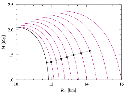
Figure 1: Left: families of rotating neutron star solutions parametrized by their central energy density, using the SLy4 equation of state and evenly spaced in polar-to-equatorial coordinate radius ratio $r_{\rm pol}/r_{\rm eq}$, from static configuration (solid, leftmost curve) to their Kepler limit (dashed, rightmost curve). As the rotation frequency increases, the stars with fixed central energy density move toward larger equatorial radii and masses. This is illustrated by the dots, which correspond to a fixed central energy density, with parameters presented in Table 1. Right: illustration of the deformation of a neutron star caused by rotation. The curves show the surface of the stars marked by a black circle in the left panel. The axes correspond to $(R/R_{\rm static})\,(1-\mu^{2})^{1/2}$ and $(R/R_{\rm static})\,\mu$. The shaded region represents a static, spherically symmetric star using the SLy4 equation of state and central total energy density $\varepsilon_{\rm c}/c^{2}=9.4769\times 10^{14}$ g/cm³, with a radius of $R_{\rm static}=11.76$ km and a mass of $M=1.35$ M_⊙. When the rotation frequency $f$ increases, the star flattens at the poles, while bulging out in the equator, as shown by the various lines. The ratio $\mathfrak{r}$ between the polar $R(1)$ to the equatorial radius $R(0)$ decreases from unity (for the static model) to $0.72$ at $f=1041.75$ Hz.

Once a neutron star solution has been obtained, we can determine the star’s coordinate surface $r_{\rm s}(\theta)$ by the loci where the pressure vanishes. Then, the (circumferential) radius of the star is determined as a function of the cosine of the colatitude $\theta$ as,

$$R(\mu)=r_{\rm s}\,e^{(\gamma_{\rm s}-\rho_{\rm s})/2}\,,$$ (2)

where we defined $\mu\equiv\cos\theta$, $\gamma_{\rm s}\equiv\gamma(r_{\rm s})$ and $\rho_{\rm s}\equiv\rho(r_{\rm s})$. Based on this definition of the surface, we also define for later use the ratio $\mathfrak{r}$

$$\mathfrak{r}\equiv{R_{\rm pol}}/{R_{\rm eq}}\,,$$ (3)

between polar radius [$R_{\rm pol}\equiv R(\mu=1)$] and equatorial radius [$R_{\rm eq}\equiv R(\mu=0)$]. We further define the eccentricity of the star as

$$e\equiv\sqrt{1-\mathfrak{r}^{2}}\,,\quad\textrm{(eccentricity)}.$$ (4)

To remain agnostic regarding the underlying matter description of neutron star interiors, we consider a set of equations of state that covers a wide variety of predicted neutron star masses and radii. The equations of state we use, in increasing order of stiffness (i.e. largest maximum mass supported) are: FPS Baym et al. (1971); Lorenz et al. (1993), SLy4 Douchin and Haensel (2001), AU Wiringa et al. (1988); Negele and Vautherin (1973), UU Wiringa et al. (1988); Negele and Vautherin (1973), APR Akmal et al. (1998) and L Pandharipande et al. (1976). Most of these equations of state are consistent with the recent gravitational wave observations of a binary neutron star coalescence by the LIGO Scientific Collaboration Abbott et al. (2018), with the exception of FPS and L, which are not stiff enough and too stiff respectively, but we include them here nonetheless for completeness. For each equation of state, we calculate 198 equilibrium configurations parametrized by the central energy density $\varepsilon_{\rm c}$ and evenly spaced in the polar-to-equatorial coordinate radii ratio $r_{\rm pol}/r_{\rm eq}$, from slowly rotating models up to the Kepler limit. In total, our catalog consists of 1188 stars.

To illustrate the impact of rotation on the properties of neutron stars, we show in the left panel of Fig. 1 the mass-(equatorial) radius relation for a family of solutions obtained using the SLy4 equation of state and various rotation rates. The solid line represents the nonrotating family of solutions, obtained by integrating the TOV (Tolman-Oppenheimer-Volkoff) equations Tolman (1939); Oppenheimer and Volkoff (1939) for a range of central energy densities $\varepsilon_{\rm c}$. The dashed lines represent families of solutions with increasing $r_{\rm pol}/r_{\rm eq}$ ratios, which is equivalent to an increase of the rotational frequency $f$. We see that the mass-(equatorial) radius relations shifts toward larger radii (due to the “bulging” out of the star’s equator) and larger masses (due to the contribution of rotational energy to the star’s gravitational mass and more support to baryons).

This behavior becomes more evident by tracking stars with constant $\varepsilon_{\rm c}$ as we increase $r_{\rm pol}/r_{\rm eq}$. As an example, in the left panel of Fig. 1 we mark with circles the solutions with $\varepsilon_{\rm c}=9.4769\times 10^{14}$ g/cm³, which show the trend described above. This particular sequence of stars covers rotation frequencies $f$ between approximately 400 and 1050 Hz, and will later serve as benchmark in our work. A variety of their properties are summarized in Table 1, and their surfaces (obtained by a procedure described in Sec. II.2) are shown in the right panel of Fig. 1.

Model	$M$	$R_{\rm eq}$	$\mathfrak{r}$	$j$	$q$	$f$	$\sigma$	$\kappa$
	($M_{\odot}$)	(km)				(Hz)
1	1.377	12.00	0.956	0.215	5.225	413.8	0.064	0.169
2	1.408	12.27	0.912	0.307	4.940	583.4	0.133	0.169
3	1.442	12.57	0.868	0.381	4.685	710.9	0.207	0.169
4	1.479	12.90	0.824	0.444	4.445	815.4	0.287	0.169
5	1.518	13.27	0.780	0.501	4.222	903.7	0.374	0.169
6	1.560	13.70	0.736	0.551	4.015	978.9	0.470	0.168
7	1.603	14.19	0.692	0.596	3.830	1041.7	0.575	0.167

Table 1: The properties of the reference stellar models. The models, obtained using the equation of state SLy4, correspond to a sequence of constant total central energy density $\varepsilon_{\rm c}=9.4769\times 10^{14}$ g/cm³ stars with increasing rotational frequency. From left to right, the columns represent the gravitational mass $M$, the equatorial radius $R_{\rm eq}$, the polar-to-equatorial radius ratio $\mathfrak{r}$, the dimensionless angular momentum $j\equiv cJ/(GM^{2})$, the dimensionless quadrupole moment $q\equiv-c^{4}Q/(G^{2}j^{2}M^{3})$, the rotational frequency $f$ and the compactness and spin parameter duo $\kappa$, $\sigma$. The surfaces of models 1, 3, 5 and 7 are shown in the right panel of Fig. 1.

In Fig. 2 we show our complete set of neutron star solutions. It is convenient to show it not in the usual mass-(equatorial) radius plane, but instead in a plane spanned by the dimensionless parameters,

$$\kappa \equiv\frac{GM}{R_{\rm eq}c^{2}}\,,\,\,\quad\textrm{(compactness)}$$ (5a)

$$\sigma \equiv\frac{\Omega^{2}R^{3}_{\rm eq}}{GM}\,,\quad\textrm{(dimensionless spin parameter)}$$ (5b)

where $\Omega=2\pi f$ is the angular frequency and we momentarily restored factors of $c$ and $G$. In this parametrization, the neutron star solutions fall on approximately equation-of-state-independent curves, whose location depends on $r_{\rm pol}/r_{\rm eq}$. If we loosely base our definition of a rapidly rotating neutron star as one with $\sigma\gtrsim 0.2$, which is approximately the value of $\sigma$ for a canonical neutron star $1.4\,{\rm M}_{\odot}$ (described by equation of state SLy4) spinning at $f\approx 716$ Hz (the frequency of the fastest known pulsar to date Hessels et al. (2006)) we see that the largest fraction of our catalog consist of rapidly rotating stars. We include very rapidly rotating stars in our work precisely because we want to study how sensitive the fitting functions that NICER uses are to their targets being slowly rotating. Currently, all NICER targets are indeed (relatively) slowly rotating (with rotational frequencies smaller than $300$ Hz Bogdanov et al. (2019a)), but in the future, it may be the case that more rapidly rotating targets are found.

What would a typical value of $\sigma$ for a NICER target be? To answer this question, we used the Markov-Chain Monte Carlo samples obtained by the Illinois-Maryland analysis of the millisecond pulsar PSR J0030+0451 Miller et al. (2019b, a), which has a known rotation frequency of $f=205.53$ Hz Lommen et al. (2000); Arzoumanian et al. (2018a). We found that the best fit value to be $\sigma=0.02$, indicating that PSR J0030+0451 is very slowly rotating in the sense described above. In this regime, neutron stars can be very well-described with the Hartle-Thorne formalism Hartle (1967); Hartle and Thorne (1968); Berti et al. (2005). In general, this formalism cannot be used to describe rapidly rotating stars, which thus forces us to rely on numerical codes such as RNS.

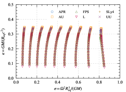
Figure 2: Neutron star models parametrized by $\sigma$ and $\kappa$ used in our analytical fits to model the stellar surface. We used an equation of state catalog that covers a wide range of stiffness. Models with fixed $\mathfrak{r}$ lie on approximately equation-of-independent-curves in this plane.

II.2 Locating the surface

Having obtained a numerical neutron star solution with RNS, how do we locate its surface? To do this, we take advantage of the first integral of the equation of hydrostationary equilibrium. The equation of hydrostationary equilibrium for a uniformly rotating star with constant angular velocity $\Omega$ is Friedman and Stergioulas (2013)

$$\frac{\nabla_{a}\,p}{(\varepsilon+p)}=\nabla_{a}\ln u^{t}\,,$$ (6)

where $u^{a}=u^{t}\,(t^{a}+\Omega\,\phi^{a})$ is the 4-velocity of a fluid element expressed in terms of the timelike and spacelike Killing vectors $t^{a}$ and $\phi^{a}$ respectively, while

$$u^{t}=\frac{\exp\left[-(\rho+\gamma)/2\right]}{\sqrt{1-(\Omega-\omega)^{2}r^{2}\sin^{2}\theta\exp(-2\rho)}}\,,$$ (7)

which follows from the normalization condition $u^{a}u_{a}=-1$ and the line element in Eq. (1).

For a barotropic equation of state, that is, one where the energy density $\varepsilon$ and pressure $p$ are related as $\varepsilon=\varepsilon(p)$, if one defines the enthalpy per unit mass as

$$h(p)\equiv\int_{0}^{p}\frac{{\rm d}p^{\prime}}{(\varepsilon+p)}\,,$$ (8)

a first integral of Eq. (6) is

$$h-\ln u^{t}=\textrm{const.}=\left(\frac{\rho+\gamma}{2}\right)_{\rm pol}\,,$$ (9)

where the right-hand side of the equation is evaluated at the pole of the star $r_{\rm pol}=r(\mu=1)$. One can verify that at the surface of the star on the pole, the enthalpy goes to zero and it is zero along the entire surface of the star, while it is positive in the interior and negative in the exterior of the star.

The RNS code provides the value of the polar redshift,

$$z_{\rm pol}=\exp\left[-(\rho_{\rm pol}+\gamma_{\rm pol})/2\right]-1\,,$$ (10)

and the surface can then be found from the condition that $h=0$ at $r=r_{\rm s}$, where the constant in (9) is $-\ln(1+z_{\rm pol})$. Next, using Eq. (7), we solve the equation

$$u^{t}(r,\mu)-z_{\rm pol}-1=0\,,$$ (11)

searching, in a sequence of values of $\mu\in[0,1]$, for the values of $r$ such that (11) is satisfied. This gives $r_{\rm s}$ and then we can find the circumferential radius using Eq. (2). A Mathematica notebook implementing these steps can be found in Pappas . As an example we show in Fig. 3 the contours of constant enthalpy per unit mass $h$ for Model 1 in Table 1. The surface is indicated with a solid line, which corresponds to $h=0$, while the two dashed lines correspond to $h=\pm 0.01$.

Figure 3: Contours of constant enthalpy per unit mass ($h$) for Model 1 of Table 1. We depict contours of constant $h=\pm 0.01$ near the surface. The contour inside the stellar surface has $h>0$ and the contour outside has $h<0$. The surface $R_{s}(\mu)$ of the star at $h=0$ is indicated by the solid line. The axes correspond to $(R/R_{\rm static})\,(1-\mu^{2})^{1/2}$ and $(R/R_{\rm static})\,\mu$, where $R_{\rm static}=11.76$ km, as in the right panel of Fig. 1.

II.3 Analytical fits

Having obtained the data for the surface $R(\mu)$ of each star in our ensemble, we can now obtain analytical fits that describe the surfaces of all stars. The procedure to generate such a formula is simple and was first explored in Morsink et al. (2007): we first fit a proposed formula $R(\mu;\{a_{n}\})$ (that depends on one or more free constants $a_{n}$) for each star, parametrized by its compactness $\kappa$ and spin parameters $\sigma$ (see Fig. 2). The outcome of this procedure is a table $\{a_{n},\,\kappa,\,\sigma\}$. This data can then be fitted to some analytical representation $a_{n}(\kappa,\,\sigma)$. These steps result in a formula $R(\mu;\{\kappa,\,\sigma\})$ for the surface.

We stress that this process introduces a smearing of the particular way in which deformations away from sphericity take place for neutron stars described by different equations of state as the rotation frequency increases. For practical applications, such as pulse profile modeling, but see also for the cooling tail method Suleimanov et al. (2017, 2020), an ideal formula $R(\mu)$ would capture accurately the neutron star surfaces at a wide range of spin frequencies, compactness and a wide set of equations of state (i.e. it has to be quasi-equation-of-state independent Morsink et al. (2007); AlGendy and Morsink (2014); Yagi and Yunes (2017)).

In the remainder of this subsection, we review two formulas used in the literature (Secs. II.3.1 and II.3.2) that share these properties and also introduce a new formula (Sec. II.3.3).

II.3.1 The Morsink et al. formula

In Morsink et al. (2007), Morsink et al. introduced a formula based on the assumption that the surface is related with the equatorial radius $R_{\rm eq}$ as

$$R_{\rm M}(\mu)=R_{\rm eq}\left[1+\sum_{n=0}^{2}a_{2n}(\sigma,\,\kappa)P_{2n}(\mu)\right]\,,$$ (12)

where $P_{\ell}(\cdot)$ are Legendre polynomials, $\mu=\cos\theta$ and $a_{2n}$ are coefficients that depend on both $\sigma$ and $\kappa$ as

$$a_{2n}\equiv c_{(1,0)}\sigma+c_{(1,1)}\sigma\kappa+c_{(2,0)}\sigma^{2}\,,$$ (13)

where $c_{(i,j)}$ is the coefficient multiplying the product $\sigma^{i}\kappa^{j}$. This notation will be used throughout this work.

The argument $\mu$ for the Legendre polynomials is chosen to enforce the $\mathbb{Z}_{2}$-symmetry of the star’s surface across the equator and the even-order Legendre polynomials are used to force that $R_{\rm M}(\mu)=R_{\rm M}(-\mu)$ across the spin axis. Up to $n=1$, this formula corresponds to the first order rotation-induced deformations in Hartle’s perturbative expansion Hartle (1967), while the $n=2$ term captures higher-order spin deformations of the star. In the nonrotating limit ($\sigma=0$), we have $a_{2}=a_{4}=0$ and therefore $R_{\rm M}=R_{\rm eq}$ for all $\mu$. One caveat of Eq. (12) is that it does not satisfy the consistency condition $R_{\rm M}(0)=R_{\rm eq}$. However, the mismatch between $R_{\rm M}(1)$ and $R_{\rm eq}$ is less than 1% Morsink et al. (2007).

The coefficients $c_{(i,j)}$ in Eq. (13) are summarized in Table 2. For self-consistency in our analysis, we recalculated the values of these coefficients using our neutron star ensemble, which differs from that used in Morsink et al. (2007) in size, rotation frequencies sampled and equations of state used. The values quoted between parenthesis in Table 2 correspond to the values found in Morsink et al. (2007). We see that in general our values are in good agreement.

Surface model		Coefficient
	$c_{(1,0)}$	$c_{(1,1)}$	$c_{(2,0)}$
Morsink et al. Morsink et al. (2007)
$a_{0}$	$(-0.18)\,-0.193$	$(+0.23)\,+0.092$	$(-0.05)\,-0.015$
$a_{2}$	$(-0.39)\,-0.391$	$(+0.29)\,+0.088$	$(+0.13)\,+0.149$
$a_{4}$	$(+0.04)\,+0.031$	$(-0.15)\,-0.064$	$(+0.07)\,+0.086$
AlGendy & Morsink AlGendy and Morsink (2014)
$a_{2}$	$(-0.788)\,-0.533$	$(+1.030)\,+0.203$	-

Table 2: Values of the coefficients $c_{(i,j)}$ for Morsink et al. and AlGendy & Morsink fits. The values quoted in parenthesis correspond to the original values found in Morsink et al. (2007); AlGendy and Morsink (2014), obtained using a neutron star ensemble different from ours. We attribute the larger differences in the AlGendy & Morsink fitting coefficients between our values and the ones quoted in AlGendy and Morsink (2014) to the fact those were obtained using a ensemble of mostly slowly rotating stars with spin parameter $\sigma\leq 0.1$, whereas we do include rapidly rotating models with $\sigma$ as large as $0.8$ (see Fig. 1).

Surface model				Coefficient
	$c_{(0,0)}^{(y)}$	$c_{(1/2,0)}^{(y)}$	$c_{(1,0)}^{(y)}$	$c_{(0,1)}^{(y)}$	$c_{(1,1)}^{(y)}$	$c_{(2,0)}^{(y)}$	$c_{(0,2)}^{(y)}$
Slow-elliptical fit
$y=e$	-	$+1.089$	$+0.168$	-	$-0.685$	$-0.802$	-
$y=a_{2}$	$-1.013$	-	$-0.312$	-	$+0.930$	$-1.596$	-
$y=a_{4}$	$+0.016$	-	$+0.301$	-	$-1.261$	$+2.728$	-
Fast-elliptical fit
$y=e$	$+0.251$	-	$+0.935$	$+0.709$	$+0.030$	$-0.472$	$-2.427$
$y=a_{2}$	$-1.265$	-	$+0.220$	$+2.651$	$+1.010$	$-1.815$	$-7.657$
$y=a_{4}$	$+0.556$	-	$-1.465$	$-4.260$	$-2.327$	$+4.921$	$+12.98$

Table 3: Values of the coefficients $c_{(i,j)}$ for the slow and fast variations of the elliptical fit. The former only uses stars for which the spin parameter is $\sigma\leq 0.25$, while the latter only those for which $\sigma\geq 0.2$.

II.3.2 The AlGendy & Morsink formula

An alternative to Eq. (12) that satisfies the constraint $R(0)=R_{\rm eq}$ was proposed by AlGendy & Morsink  AlGendy and Morsink (2014) and is currently in use in the pulse profile modeling by NICER Bogdanov et al. (2019b). Their formula is

$$R_{\rm A}(\mu) =R_{\rm eq}\left[1-\left(1-\mathfrak{r}\right)\,\mu^{2}\right]\equiv R_{\rm eq}\left[1+a_{2}(\kappa,\sigma)\,\mu^{2}\right]\,,$$

where the coefficient $a_{2}$ is given by

$$a_{2}=c_{(1,0)}\sigma+c_{(1,1)}\sigma\kappa\,,$$ (15)

and represents the multiplicative factor $(1-\mathfrak{r})$, which contains both the equatorial $R_{\rm eq}$ and polar $R_{\rm pol}$ radii of the star [cf. Eq. (3)]. Due to the same symmetry requirements as in the Morsink et al. fit, even powers of $\mu=\cos\theta$ are used. In the nonrotating limit $(\sigma=0)$, $a_{2}=0$ and therefore $R_{\rm A}=R_{\rm eq}$ for all $\mu$.

The values of $c_{(1,0)}$ and $c_{(1,1)}$ are quoted in Table 2. As we did previously for the Morsink et al. formula, we recalculated the fitting coefficients using our own neutron star ensemble. We find larger differences between our values and those quoted in AlGendy and Morsink (2014). We credit these differences due to the fact that Ref. AlGendy and Morsink (2014) only considered slowly rotating stars ($\sigma\leq 0.1$) whereas our catalog consists of mostly rapidly rotating stars ($\sigma\geq 0.25$), as we have discussed before.

II.3.3 The elliptical formula

In addition to the models previously described, we also introduce a new expression. Our choice is inspired by the elliptical isodensity approximation Lai et al. (1993) and is given by:

$$R_{\rm E}(\mu)=R_{\rm eq}\sqrt{\frac{1-e^{2}}{1-e^{2}\,g(\mu)}}\,,$$ (16)

where

$$g(\mu) =1+a_{2}(\kappa,\sigma)\,\mu^{2}+a_{4}(\kappa,\sigma)\,\mu^{4}$$

$$\quad-[1+a_{2}(\kappa,\sigma)+a_{4}(\kappa,\sigma)]\,\mu^{6}\,.$$ (17)

and the term multiplying $\mu^{6}$ was chosen such that,

$$\frac{R_{\rm E}(1)}{R_{\rm E}(0)}=\mathfrak{r}=\sqrt{1-e^{2}}\,,$$ (18)

thereby enforcing the interpretation of $e$ as the star’s eccentricity Stein et al. (2014). As in the previous fitting formulas, even powers of $\mu$ are used to enforce $R_{\rm E}(\mu)=R_{\rm E}(-\mu)$. At a qualitative level our formula differs from Eqs. (12) and (LABEL:eq:fit_algendy_etal) in that we are including relativistic and spin corrections to an otherwise ellipsoidal star, whereas the other two fits are including relativistic and spin corrections to an otherwise spherical star. Using an ellipsoidal star as the unperturbed configuration is motivated by the fact that in Newtonian gravity rotating stars are not spheres, but rather they are ellipsoids of revolution.

We obtained two fits using our elliptic formula. The first, which we name the “slow elliptical” fit, uses only stars with $\sigma\leq 0.25$. The second, which we name the “fast elliptical” fit, uses only stars with $\sigma\geq 0.2$. The reasons are twofold. First, on the observational side, the fastest known millisecond pulsar has a frequency of 716 Hz Hessels et al. (2006), which is approximately 2.5 times the rotation frequency of the fastest spinning NICER’s target Bogdanov et al. (2019a), PSR J1231–1411 which has a rotation frequency of $271.7$ Hz Ransom et al. (2011). Second, on the practical side, the majority of the stars in our catalog have $\sigma>0.25$, which corresponds approximately to minimum rotation frequencies in the 700-800 Hz range. Therefore, any fit obtained using the full catalog will be skewed toward the values of coefficients $c_{(i,j)}$ corresponding to rapidly rotating stars. These two observations suggest separating our fits in the slow and fast fits, including a “buffer $\sigma$-region” where they overlap.

The coefficients $e$, $a_{2}$ and $a_{4}$ are determined by

$$y =c_{(0,0)}^{(y)}+c_{(1/2,0)}^{(y)}\sigma^{1/2}+c_{(1,0)}^{(y)}\sigma+c_{(0,1)}^{(y)}\kappa$$

$$\quad+c_{(1,1)}^{(y)}\sigma\kappa+c_{(2,0)}^{(y)}\sigma^{2}+c_{(0,2)}^{(y)}\kappa^{2}\,,$$ (19)

with $y$ any of $e$ or $a_{2n}$. In the slow-elliptical fit we set

$$c_{(0,0)}^{(e)}=c_{(1,0)}^{(e)}=c_{(2,0)}^{(e)}=0\,,$$ (20a)

$$c_{(1/2,0)}^{(a_{2n})}=c_{(1,0)}^{(a_{2n})}=c_{(2,0)}^{(a_{2n})}=0\,,$$ (20b)

since to impose the nonrotating limit we must set all $\sigma$-free coefficients to zero. The peculiar fractional-order coefficient $c_{(1/2,0)}$ is introduced to capture better the behavior of the eccentricity $e$ in the $\sigma\ll 1$ limit. As for the fast-elliptical fit, we do not need to impose these restrictions on the $\sigma$-free coefficients, but we do set

$$c_{(1/2,0)}^{(y)}=0,\quad\textrm{for}\quad\,y=\{e,\,a_{2n}\}\,,$$ (21)

since its introduction was motivated by $e$ in the small-$\sigma$ limit. The coefficients $c_{(i,j)}$ for both flavors of the elliptic fit are summarized in Table 3.

II.4 Comparison between the different formulas

In the previous section, we introduced three formulas that describe the surface of neutron stars for a wide range of spin and compactness parameters. How do they compare when confronted against the properties of individual neutron star models computed as accurately as possible? Neutron stars are generally believed to be described by a single equation of state. Therefore, using fits which integrate out the surface variability of neutron stars due to different equations of state could introduce a source of systematic error in any neutron star parameter estimation where the fits are used.

As a first step to analyze this source of systematic error, in this section we compare the three formulas (using our own fitting coefficients) against neutron star models computed numerically with the equation of state SLy4 Douchin and Haensel (2001). We use our own fitting coefficients for all three formulas to avoid a systematic error introduced by comparing different fits obtained from different neutron-star catalogs. Recall that the catalogs used here and in Refs. Morsink et al. (2007); AlGendy and Morsink (2014) are all different. We chose the equation of state SLy4 because it yields neutron stars with masses greater than $1.9\,{\rm M}_{\odot}$ as required by the observations of the massive pulsars J1614$-$2230 Demorest et al. (2010); Fonseca et al. (2016); Arzoumanian et al. (2018b), J0348+0432 Antoniadis et al. (2013) and J0740+6620 Cromartie et al. (2019), and yet it is relatively soft as required by tidal deformability estimates from the GW170817 event Abbott et al. (2017, 2018, 2019).

Let us first describe the neutron star models we will use as benchmarks in this section and in the remainder of this work. We use a sequence of stars parametrized by their central energy density $\varepsilon_{\rm c}$ ($=9.4769\times 10^{14}$ g/cm³), which for the SLy4 equation of state results results in a “canonical” neutron star with a mass of approximately $1.4\,{\rm M}_{\odot}$ in the nonrotating limit. The properties of these “benchmark stars” are summarized in Table 1 and they are indicated by markers in the mass-(equatorial) radius plane in Fig. 1. We will use the term “benchmark” to any property or observable calculated using one of these stars. For instance, we will refer to their surfaces as “benchmark surfaces” and to the pulse profile emitted from their surface as “benchmark pulse profiles.”

To describe the shape of these stars as accurately as possible we fit separately both $R=R(\mu$) and

$$\frac{{\rm d}\log R(\mu)}{{\rm d}\theta}=-(1-\mu^{2})^{1/2}\frac{1}{R(\mu)}\frac{{\rm d}R(\mu)}{{\rm d}\mu}\,,$$ (22)

the latter being a measurement of the deviation from sphericity of the star’s surface and subject to the constraints

$$[{\rm d}\log R(\mu)/{\rm d}\theta]_{\mu=0}=[{\rm d}\log R(\mu)/{\rm d}\theta]_{\mu=1}=0\,.$$ (23)

Model	$10^{-2}\cdot a_{2}$	$10^{-2}\cdot a_{4}$	$10^{-2}\cdot a_{6}$	$10^{-2}\cdot a_{8}$	$10^{-2}\cdot a_{10}$	$10^{-2}\cdot b_{1}$	$10^{-2}\cdot b_{3}$	$10\cdot c_{0}$	$10\cdot c_{2}$	$10\cdot c_{4}$
1	$-4.174$	$0.3647$	$-0.0495$	$0.01175$	$-0.0034$	$-5.213$	$-5.623$	$6.244$	$7.575$	$0.811$
2	$-9.132$	$1.832$	$-0.531$	$0.1603$	$-0.0310$	$-10.42$	$-10.67$	$5.702$	$7.656$	$1.464$
3	$-15.15$	$5.349$	$-2.644$	$1.173$	$-0.276$	$-18.16$	$-12.09$	$5.992$	$7.373$	$1.403$
4	$-22.68$	$12.73$	$-9.303$	$5.279$	$-1.422$	$-19.50$	$-17.04$	$4.295$	$7.769$	$1.895$
5	$-32.44$	$27.49$	$-27.20$	$18.32$	$-5.423$	$-17.76$	$-23.03$	$2.724$	$7.710$	$2.603$
6	$-45.69$	$56.56$	$-70.98$	$54.16$	$-17.17$	$-16.07$	$-30.44$	$1.731$	$7.760$	$3.507$
7	$-64.72$	$114.0$	$-172.8$	$145.0$	$-48.43$	$-13.76$	$-38.70$	$1.013$	$7.644$	$4.591$

Table 4: Values of the coefficients $a_{i}$ in the fitting formula Eq. (24a) and $b_{i}$, $c_{i}$ in Eq. (24b) for our set of reference stellar models, whose properties are summarized in Table 1.

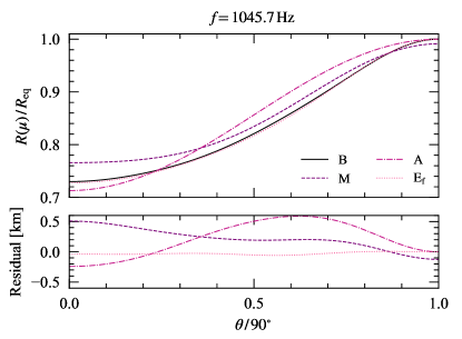
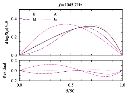
Figure 4: Surfaces (top) and surficial logarithmic derivative (bottom) of rotating neutron stars. The left-panels correspond to a star with rotation frequency of $f=413.8$ Hz, whereas the right-panels to a star with rotation frequency of $f=1045.7$ Hz, which correspond to the benchmark stars labeled 1 and 7 in Table 1. The top-panels show $R(\mu)$ normalized by the equatorial radius $R_{\rm eq}$, while the bottom panels show ${\rm d}\log R(\mu)/{\rm d}\theta$ without normalization. The different curves correspond to the surface as determined by the RNS code (solid line), as predicted using the Morsink et al. fit (dashed line), the AlGendy & Morsink fit (dash-dotted line) and the elliptical fit (dotted lines), with the slow-elliptical fit on the left and the fast-elliptical fit on the right. The bottom panels show the residuals between each of the fits and the benchmark surfaces.

For these two quantities we used the following fitting formulas

$$R_{\rm B}(\mu) =R_{\rm eq}\left(1+\sum_{k=1}^{5}a_{2k}\mu^{2k}\right)\,,$$ (24a)

$$\frac{{\rm d}\log R_{\rm B}(\mu)}{{\rm d}\theta} =-(1-\mu^{2})^{1/2}\frac{\sum_{k=0}^{2}b_{2k+1}\mu^{2k+1}}{\sum_{k=0}^{3}c_{2k}\mu^{2k}}\,.$$ (24b)

Equation (24a) is a higher-order AlGendy & Morsink fit, with the higher powers of $\mu$ introduced to describe the greater deformations away from spherical symmetry that happen at high rotation frequencies and to simultaneously retain the property that $R_{\rm B}(0)=R_{\rm eq}$. Equation (24b) is chosen such as to represent the logarithmic derivative of Eq. (24a) and, by construction, it satisfies the constraints of Eq. (23).

We used these formula to fit our numerical data and the resulting fitting coefficients $a_{i}$, $b_{i}$ and $c_{i}$ are summarized in Table 4. To obtain the fits for Eq. (24b), we first calculated numerically the logarithmic-derivative using a sixth-order finite difference formula. A detailed study of the numerical derivatives and the goodness of the fits is presented in Appendix A.

In the top panel of Fig. 4 we show the residuals $R_{\rm fit}-R_{\rm B}$, as functions of the colatitude $\theta$, between the three fitting formulas and the benchmark stars for the slowest and fastest rotating stars in Table 1. We see that for the slowest rotating model (left-panel) the Morsink et al. and the (slow) elliptic fit behave very similarly and they are both closer to the benchmark surface in comparison to the AlGendy & Morsink formula. Nonetheless, the residuals are small, below $0.1$ km, indicating that all three formulas agree well with the benchmark surface. The situation changes when we consider the fastest rotating model (right-panel). We see that the (fast) elliptical fit outperforms both the Morsink et al. and the AlGendy & Morsink fits. For the latter two formulas the largest value of the residual increases approximately fivefold, however, staying bound to be less than 0.5 km. In the bottom panel of Fig. 4 we carry out the same analysis but for the logarithmic-derivative of the surface, reaching similar conclusions.

III Implications of the fitting formulas on the pulse profiles

In the previous section we introduced the various fitting expressions for the surface of rotating neutron stars and studied how well they reproduce a set of benchmark surfaces. How does the mismatch between fit and benchmark surfaces appear in the pulse profile generated by hot spots on the star’s surface? In this section we address this question in two fronts. First, given that the surface depends on the colatitude $\theta$, it is clear that the mismodeling of pulse profiles will depend both on where on the surface the hot spot is located ($\theta_{\rm s})$ and on the line of sight of the observer ($\iota_{\rm o}$), where both angles measured relative to the rotation axis of the star. Therefore, it is natural to examine for which combinations $(\theta_{\rm s},\,\iota_{\rm o})$ the mismatch is smallest/largest. Second, we want to explore how the different formulas perform when trying to extract the equatorial radius $R_{\rm eq}$ from a synthetic injection. Of course, both questions are intertwined as, for instance, a combination $(\theta_{\rm s},\,\iota_{\rm o})$ for which the flux mismatch is large will, likely, result in a large systematic error in the inference of $R_{\rm eq}$. For the reasons explained in Sec. II.4, we continue to use the surface formulas with our own set of fitting coefficients.

To answer these questions we need to construct (as accurately as possible) reference pulse profiles to compare against. Ideally, these “benchmark pulse profiles” should be calculated doing ray-tracing on a numerically constructed rotating neutron star spacetime. For simplicity, we restrict ourselves to the O+S model, with the star’s oblateness modeled by the high-order fitting expressions introduced in Sec. II.4.

As already mentioned, the O+S model is currently used by NICER and its validity has extensively been examined by comparison against ray-tracing in numerically obtained spacetimes of rotating neutron stars. These studies have shown that the O+S model can accurately describe the x-ray emission of the neutron star surfaces for a typical NICER target. Our own implementation of the O+S model follows closely the presentation in Refs. Morsink et al. (2007); Salmi et al. (2018); Bogdanov et al. (2019b). The code was validated against the Alberta code described in Bogdanov et al. (2019b) which, in turn, has been validated against several other codes used in the NICER collaboration.

In all calculations in this work, we assume for simplicity a pointlike hot spot with angular radius $\Delta\theta_{\rm s}=0.01^{\circ}$. We further assume that this hot spot radiates isotropically according to a blackbody spectrum with $k_{\rm B}T^{\prime}_{0}=0.35$ keV (measured by an observer comoving with the hot spot). We place the observer at a distance $d=200$ pc from the source and we assume that this observer collects photons arriving with $E=1$ keV. We also fix the initial phase of the observed flux (i.e. its zero value) to when the hot spot is closest to the observer. This is a representative value within the soft x-ray band in which NICER operates. These quantities are summarized in Table 5.

Parameter	Value
Hot spot angular radius ($\Delta\theta_{\rm s}$)	$0.01$ deg
Hot spot temperature at comoving frame ($k_{\rm B}T^{\prime}_{0}$)	$0.35$ keV
Observed photon energy ($E$)	1 keV
Distance ($d$)	200 pc

Table 5: Pulse profile parameters. The table summarizes the parameters that enter the pulse profile calculation which we keep fixed throughout this work. We assume the existence of single, pointlike hot spot on the star’s surface to isolate the effects of the different neutron star surface models on the resulting x-ray flux.

These simplifications allow us to isolate the influence of the different surface models on the pulse profiles. However, our results must be considered conservative since other effects, such as the influence of frame dragging and higher-spacetime multipole moments on the photon motion, are not taken into account in the O+S approximation. Our analysis, while indicative of what can happen in a more complete analysis, cannot substitute a full parameter estimation in the framework of Bayesian inference (see, e.g., Lo et al. (2013, 2018); Miller (2016); Miller et al. (2019a); Riley et al. (2019)), a task which we leave for future study.

In Fig. 5 we show some examples of the difference in the pulse profile (in units of photons cm^-2 s^-1 keV^-1) when we fix all parameters used to produce it and only vary the fitting formula used to model the star’s surface. We quantify this difference by subtracting the benchmark pulse profile (i.e. the one obtained using the “exact” surface formula) from the pulse profile obtained using each fitting formula and then dividing by the mean value of the former. We consider the slowest and fastest stars in our benchmark catalog and two hot spot-observer orientations. The first, labeled “low inclination” has $(\theta_{\rm s},\,\iota_{\rm o})=(45^{\circ},\,20^{\circ})$, while the second, labeled “high inclination” has $(\theta_{\rm s},\,\iota_{\rm o})=(80^{\circ},\,85^{\circ})$. These two configurations are summarized in Table 6. The figure shows that for the slowest rotating model, all fitting formulas agree with the benchmark pulse profiles with differences of at most $\sim 1\%$. For the fastest rotating model, a larger differences appear and can be as large as $\sim 30\%$. Except at these phase values, all formulas agree with the benchmark pulse profile in the high-inclination case. However, for the low-inclination case, we see that the new fast elliptical fit does agree remarkably well with the benchmark pulse profile.

Case	$\theta_{\rm s}$	$\iota_{\rm o}$	$\delta{R_{\rm eq}}$
	(deg)	(deg)	(km)
Low inclination	45	20	0.20
High inclination	80	85	0.05

Table 6: Summary of the hotspot/observer arrangements used in the estimation of $R_{\rm eq}$ and the values of the statistical error $\delta{R_{\rm eq}}$ used when calculating the likelihood. The two arrangements are located Fig. 6 by the markers $\bigcirc$ (low inclination) and $\Box$ (high inclination). The statistical errors are based on Lo et al. (2013, 2018).

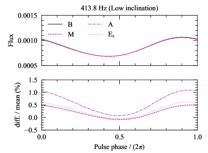
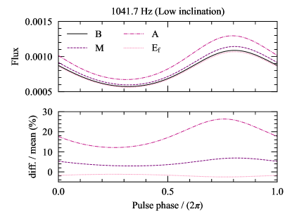
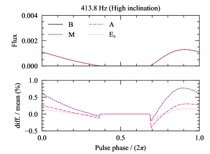
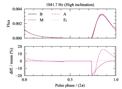
Figure 5: Illustrative pulse profiles. We compare the pulse profiles, in units of photons cm^-2 s^-1 keV^-1, obtained using the three different fitting formulas against those obtained by the slowest and fastest rotating benchmark stars (models 1 and 7 in Table 1). Top row: the low-inclination hot spot/observer orientation with the pulse profiles in the top panel and the difference between each surface model and the benchmark pulse profiles divided by the mean of the latter in the bottom panel. Bottom row: similar to the top row but for the high-inclination hot spot-observer orientation.

III.1 Dependence on the hot spot and observer’s orientation

Let us examine the error introduced by the fitting formulas, relative to the benchmark pulse profiles, when we vary the hot spot ($\theta_{\rm s}$) and observer location ($\iota_{\rm o}$). The reason for this study is the following: there is no reason for the error to be the same for all pairs $(\theta_{\rm s},\iota_{\rm o})$. Indeed, as shown in Fig. 4, a surface fit can match exactly the benchmark models locally, although not well globally. If the hotspot is located at one of these special values of colatitude, the resulting pulse profile will be the same. The location of these “coincident colatitudes” depends on the frequency $f$ of the star. For instance, returning to Fig. 4, we see that for the AlGendy & Morsink fit this happens at $\theta/90^{\circ}=1$ when $f=413.8$ Hz, but at $\theta/90^{\circ}\approx 0.32$ and $1$ when $f=1045.7$ Hz. An extreme example where this situation happens for all rotation frequencies is when both $\theta_{\rm s}$ and $\iota_{\rm o}$ are on the equator ($90^{\circ}$). In this case, as long as $R_{\rm fit}=R_{\rm eq}$ the pulse profiles will be identical. This happens for the AlGendy & Morsink and elliptical fits, and to a good approximation for the Morsink et al. formula.

We quantify the mismatch between pulse profiles predicted by the different surface formulas over the course of a single revolution of the star using two measures. First, we define the mean residual

$$\mathscr{R}\equiv\frac{1}{N_{\rm bins}}\,\sum_{i=1}^{N_{\rm bins}}|F^{\rm B}_{i}-F^{\rm fit}_{i}|\,,$$ (25)

where $F^{\rm B}_{i}$ ($F^{\rm fit}_{i})$ is the flux calculated using the benchmark surface (the fitting formulas) at the $i$-th phase bins and $N_{\rm bins}=16$ is total number of phase bins used. Second, we define the “normalized” residual

$$\mathscr{M}\equiv\frac{1}{N_{\rm bins}}\frac{\sum_{i=1}^{N_{\rm bins}}|F^{\rm B}_{i}-F^{\rm fit}_{i}|}{\langle F^{\rm B}\rangle}\,,$$ (26)

where $\langle F^{\rm B}\rangle$ is the mean value of the benchmark pulse profile,

$$\langle F^{\rm B}\rangle\equiv\frac{1}{N_{\rm bins}}\,\sum_{i=1}^{N_{\rm bins}}F^{\rm B}_{i}\,.$$ (27)

In Fig. 6, we show $\mathscr{M}$ as a function of ($\theta_{\rm s},\iota_{\rm o}$) in the domain $\mathscr{D}=[0,90^{\circ}]\times[0,90^{\circ}]$, for four sample benchmark stars with rotation frequencies $413.8$, $710.9$, $903.7$ and $1041.7$ Hz. These correspond to the stars labeled 1, 3, 4 and 7 in Table 1. These four stars define the columns in Fig. 6, while the four fitting formulas define the rows. We use the same color map scale along each column. This figure reveals a number of interesting facts, namely:

• As expected, the normalized residual is minimal at $\theta_{\rm s}=\iota_{\rm o}=90^{\circ}$. In fact, it remains small for any $\iota_{\rm o}$, as long as $\theta_{\rm s}\approx 90^{\circ}$, for all formulas.

• The Morsink et al. , AlGendy & Morsink and (slow) elliptical formulas all have small normalized residuals for all combinations of $\theta_{\rm s}$ and $\iota_{\rm o}$ relative to the benchmark flux at $413.6$ Hz (leftmost column). Since this value is already larger than the fastest spinning neutron star in NICER’s target list, we can expect that these three formulas would imply similar best fit parameter estimates if used to analyze NICER data. Perhaps unsurprisingly, the fast-elliptical fit (which was obtained using only $\sigma\geq 0.25$ stars) has regions in the $(\theta_{\rm s},\,\iota_{\rm o})$ where the normalized residual becomes larger ($\mathscr{M}\geq 0.3$). Yet, these regions are confined to $\theta_{\rm s}\leq 25^{\circ}$.

• For faster rotating stars (the three rightmost columns), we see that the Morsink et al. , AlGendy & Morsink and slow elliptical formulas start to fail to reproduce the benchmark flux, as can be seen by the increase in size of the region in which $\mathscr{M}\gtrsim 0.3$. There are regions however, where the normalized residual still remains small. In contrast, the fast elliptical formula outperforms all the three formulas when applied to rapidly rotating stars, as we should expect, by construction.

In Fig. 7 we show the dimensionless integrated values of $\mathscr{M}$, defined as

$$\bar{\mathscr{M}}\equiv\int_{\mathscr{D}}\mathscr{M}\,{\rm d}(\theta_{\rm s}/90^{\circ})\,{\rm d}(\iota_{\rm o}/90^{\circ})\,,$$ (28)

(and likewise for $\bar{\mathscr{R}}$) as a function of the rotation frequency $f$ for the seven benchmark stars. The figure shows that these two error measures behave similarly. For the Morsink et al. , AlGendy & Morsink and slow-elliptical fits, both $\bar{\mathscr{R}}$ and $\bar{\mathscr{M}}$ increase monotonically as a function of $f$. On the other hand, for the fast-elliptical fit both $\bar{\mathscr{R}}$ and $\bar{\mathscr{M}}$ decrease with $f$ to values smaller than the other three curves, yet showing a small oscillatory behavior past 700 Hz, probably associated with numerical error.

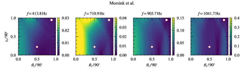
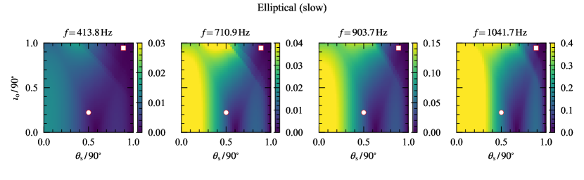
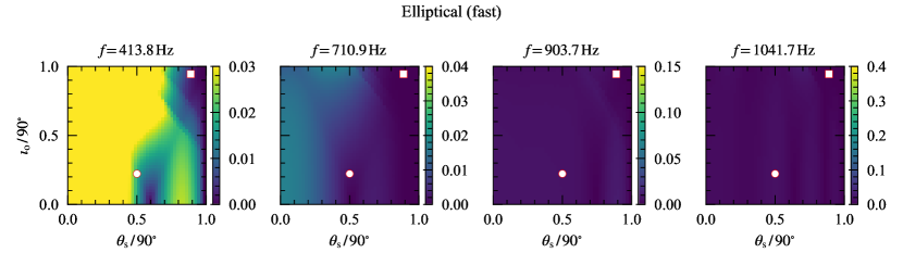
Figure 6: The normalized residual $\mathscr{M}$ [defined in Eq. (26)] as function of ($\theta_{\rm s}$, $\iota_{\rm o}$). The results for $\mathscr{R}$ [defined in Eq. (25)] are qualitatively the same. We use the same scale for all panels in each column. The columns correspond to which benchmark star we compared each fitting formula against. We see that as the rotation frequency $f$ increases the Morsink et al. (top row) and AlGendy & Morsink (middle row) in general deteriorate relative to our benchmark fluxes, calculated using the formulas of Sec. II.4. On the other hand, the elliptic fit remains relatively accurate for the whole frequency range considered by us. This conclusion can be quantified by calculating the integrals of $\mathscr{M}$ and $\mathscr{R}$, whose results are shown in Fig. 7. The markers denote the two combinations of hot spot colatitude ($\theta_{\rm s}$) and line of sight to the observer ($\iota_{\rm o}$) angles used in our parameter estimation study in Sec. III.2.2.

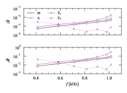
Figure 7: The integrated values of $\bar{\mathscr{R}}$ (top panel) and $\bar{\mathscr{M}}$ (bottom panel) in the domain shown in Fig. 6 as functions of the rotation frequency $f$ of the benchmark stars. The legend is shared between both panels. Overall, all three formulas perform well for slowly rotating stars. As the rotation frequency $f$ increases, the errors for the Morsink et al. (solid lines) and AlGendy & Morsink (dashed lines) fits increase, whereas for the elliptic fit (dash-dotted line) the errors show less variability.

III.2 Systematics errors on the equatorial radius inference

In this section we study how the different formulas used to describe surface of rotating neutron stars affect the parameter estimation of the star’s equatorial radius. We continue to use the simplifying assumptions of Sec. III and the parameters summarized in Table 5. We further fix the orientation angles $(\theta_{\rm s}$, $\iota_{\rm o})$ according to the two cases listed in Table 6. Finally, the star parameters $M$, $R_{\rm eq}$ and $f$ are fixed to:

• $M=1.4$ M_⊙, $R_{\rm eq}=13$ km and $f=205$ Hz as to mimic the parameters inferred from PSR J0030+0451 Miller et al. (2019a). We use the AlGendy & Morsink formula to describe the star’s surface. (Section III.2.2.)

• $\{M,\,R_{\rm eq},\,f\}$ are those of the benchmark stars of Table 1. We use the benchmark surface models of Sec. II.4.

In both cases, we use the same methodology to perform a (restricted) likelihood analysis study as used in Silva and Yunes (2019).

III.2.1 Statistical methods

We call the signal measured during an observation the synthetic injected signal, or (for brevity) the injection $F_{\rm inj}(\bm{\vartheta}^{\ast})$. The pulse profile that we use to extract and characterize this observed pulse profile is referred to as the model $F_{\rm mod}(\bm{\vartheta})$. Here, ${\bm{\vartheta}^{\ast}}$ (${\bm{\vartheta}}$) represent the injection (model) parameters used to calculate the pulse profile.

Both pulse profiles are calculated using the O+S approximation once all parameters

$$\bm{\vartheta}=\{M,R_{\rm eq},f,\theta_{\rm s},\iota_{\rm o},\Delta\theta_{\rm s},d,k_{\rm B}T^{\prime}_{0}\}\,,$$ (29)

have been specified. As done in the previous section, we work with a reduced model parameter space obtained by fixing

$$\bm{\vartheta}_{\rm fix}=\{M,f,\theta_{\rm s},\iota_{\rm o},\Delta\theta_{\rm s},d,k_{\rm B}T^{\prime}_{0}\}\,,$$ (30)

to the injected values, leaving as the single variable parameter the equatorial radius $R_{\rm eq}$.

We calculate the best-fit parameter value by minimizing the reduced chi-squared $\chi^{2}_{\rm red}$ between the injection and the model pulse profiles, sampling over the model’s variable parameter $R_{\rm eq}$. The reduced chi-squared is defined as

$$\chi_{\rm red}^{2}\equiv\frac{1}{N}\sum_{i=1}^{N}\left[\frac{F_{\rm mod}(\phi_{i},{\bm{\vartheta}}_{\rm fix},R_{\rm eq})-F_{\rm inj}(\phi_{i},{\bm{\vartheta}}_{\rm fix},R_{\rm eq}^{\ast})}{\sigma(\phi_{i})}\right]^{2}\,,\\$$ (31)

where $R^{\ast}_{\rm eq}$ is the equatorial radius of the star used to calculate the injection pulse profile. The summation in (31) is over the $N$ time stamps during the course of one observed revolution of the star. We normalize the phase (dividing by $2\pi$) for a revolution such that $\phi_{i}\in[0,1]$ and use $N=16$ time stamps. The standard deviation of the distribution ($\sigma$) is modeled as $\sigma(\phi_{i})=\sigma_{R_{\rm eq}}(\phi_{i})$, where $\sigma_{R_{\rm eq}}$ is the standard deviations on the (injection) equatorial radius. We calculate the standard deviation $\sigma_{R_{\rm eq}}$ as Ayzenberg et al. (2016); Ayzenberg and Yunes (2017).

$$\sigma_{R_{\rm eq}} =\frac{1}{2}\left|F_{\rm inj}(\phi_{i},{\bm{\vartheta}}_{\rm fix},R_{\rm eq}^{\ast}+\delta R_{\rm eq})\right.$$

$$\quad\left.-\,\,F_{\rm inj}(\phi_{i},{\bm{\vartheta}}_{\rm fix},R_{\rm eq}^{\ast}-\delta R_{\rm eq})\right|\,,$$ (32)

where we assume the values for the statistical error $\delta R_{\rm eq}$ listed in Table 6. To obtain the standard deviation, we need to calculate the pulse profile emitted by a star with radii $R^{\ast}_{\rm eq}\pm\delta R_{\rm eq}$. In this calculation, we cannot use the “exact” fits (because they are valid only for the benchmark stars), nor the fitting formulas we are using to calculate the model pulse profile $F_{\rm mod}$ (because it could bias the resulting likelihood). To overcome this problem, we obtained a high-order AlGendy & Morsink fit, similar to Eq. (LABEL:eq:fit_algendy_etal) but adding terms $a_{2i}\,\mu^{2i}$ up to $i=5$ and using only stars described by the SLy4 equation of state.

Once the reduced chi-squared is obtained, we assume that the likelihood is Gaussian

$$L(R_{\rm eq})=\exp\left(-\chi_{\rm red}^{2}/2\right)\,,$$ (33)

which we combine with the prior $\pi(R_{\rm eq})$, to obtain the posterior

$$P(R_{\rm eq})\propto L(R_{\rm eq})\cdot\pi(R_{\rm eq})\,.$$ (34)

We use a flat prior in the range $\kappa\in[0.125,0.3125]$ for the compactness Miller et al. (2019a). We also set an upper bound on the spin parameter, $\sigma\leq 1$, a condition that is only violated by stars rotating near their mass-shedding frequency. These two conditions combined with the fixed mass $M$ and rotational frequency $f$ of the star (used to produce the injection pulse profile) fix a range of values for $R_{\rm eq}$. We take our prior on $R_{\rm eq}$ to be uniform in the range $R_{\rm eq}\in[10,\,R_{\rm eq}^{\rm max}]$ km, where the upper bound is set by the lower and upper limits on $\kappa$ and $\sigma$ respectively.

In Fig. 8 we illustrate this discussion. The solid lines delimit the allowed region in the ($M$, $R_{\rm eq}$)-plane by the compactness prior alone. Part of this region is carved out by imposing an upper limit on $\sigma$ which, for four sample values of $f$, are shown by the dashed lines. We see that for the slowest rotating star in Table 1 (for which $1.377$ M_⊙ and $f=413.8$ Hz) the value of $R_{\rm eq}^{\rm max}$ is set by the lower prior on the compactness ($\kappa=0.125$). On the other extreme, for the fastest rotating star (for which $1.603$ M_⊙ and $f=1041.7$ Hz), the value of $R_{\rm eq}^{\rm max}$ is set by the upper bound on the spin parameter ($\sigma=1$ with $f\approx 1041$ Hz). The prior ranges on $R_{\rm eq}$ for these two examples are illustrated by the dot-dashed lines labeled “1” and “7”, respectively.

To obtain the posterior distribution $P(R_{\rm eq})$, we evaluate Eq. (34) on a fine grid covering $R_{\rm eq}\in[10,\,R^{\rm max}_{\rm eq}]$ km. Next, we sort the pair $\{R_{{\rm eq},i},\,P(R_{{\rm eq},i})\}$ in an descending order of posterior. The first entry determines the best fit inferred value of the equatorial radius. We are also interested in the $1\sigma$ credible intervals of the resulting posterior distributions. To calculate them, we add all $P(R_{{\rm eq},i})$-values until the cumulative sum reaches 68% of the total $\sum_{i}^{N}P(R_{{\rm eq},i})$. The smallest and largest values of $R_{{\rm eq},i}$ in this interval yield the credible interval.

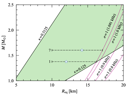
Figure 8: Lines of constant compactness ($\kappa$) and spin parameter ($\sigma$) in the mass-equatorial-radius plane. The two solid lines correspond to the edges of the prior range on the compactness. The four dashed lines mark curves of constant $\sigma=1$ for some sample rotational frequency values: $f=$ 800, 900, 1000 and 1041 Hz. For stars with $M\lesssim 1.4$ M_⊙, the lower end of the prior ($\kappa=0.125$), fixes the largest allowed value of the equatorial radius $R^{\rm max}_{\rm eq}$. For stars with larger masses, the upper limit $\sigma\leq 1$, reduces $R^{\rm max}_{\rm eq}$ if the rotation frequency $f$ is sufficiently high. Both scenarios are illustrated by the dot-dashed lines labeled 1 and 7, which make reference to the labels used in Table 1. For the line labeled 1, the mass is $1.377$ M_⊙ and $f=413.8$ Hz and thus $R_{\rm eq}^{\rm max}$ is set by lower end of the prior in the compactness. Conversely, for the line labeled 7, the mass is $1.603$ M_⊙ and $f=1041.7$ Hz and thus $R_{\rm eq}^{\rm max}$ is set by the $\sigma=1$ ($f=1041.7$ Hz) curve. The values of $R_{\rm eq}$ and $M$ of the benchmark stars 1 and 7 are marked with stars.

III.2.2 Systematics due to fitting formulas

In this section, we calculate our injection flux using the AlGendy & Morsink model for the star surface, assuming $M^{\ast}=1.4$ M_⊙, $R_{\rm eq}^{\ast}=13$ km and $f^{\ast}=205$ Hz. These values were chosen to mimic a source similar to PSR J0030+0451 as inferred by the Illinois-Maryland analysis Miller et al. (2019a). We are interested in whether the other formulas (Morsink et al. and elliptical) can recover the injected equatorial radius.

In Fig. 9 we show the resulting posterior distributions on $R_{\rm eq}$ obtained from this exercise, which we did for the two hot spot-observer orientations of Table 6. The posteriors clearly show that the best fit values of $R_{\rm eq}$ for both Morsink et al. (solid lines) and the two flavors of the elliptical formulas (dot-dashed and dashed lines) agree well with the injection $R_{\rm eq}^{\ast}$ (vertical dotted line).

These results are hardly surprising given our discussion in Sec. III.1 but serve (albeit through a restrictive likelihood analysis) to show that all three formulas work equally well in describing the pulse profile emitted by neutron stars targeted by NICER, i.e. millisecond pulsars with rotation frequencies below a few hundred hertz Bogdanov et al. (2019a).

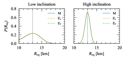
Figure 9: Posterior probability distributions of the equatorial radius. Left panel: for the low-inclination ($\theta_{\rm s}=45^{\circ}$, $\iota_{\rm o}=20^{\circ}$) orientation. Right panel: for the high-inclination ($\theta_{\rm s}=85^{\circ}$, $\iota_{\rm o}=80^{\circ}$) orientation. Pulse profile models using both the Morsink et al. (solid lines) and the elliptic fits (dashed and dot-dashed lines) recover the injected radius $R_{\rm eq}^{\ast}=13$ km (vertical dotted line).

III.2.3 Systematics due to equation of state averaging

We now turn our attention to the systematic errors that may be introduced by the fact that the surface formulas represent an average of the shape of an ensemble of neutron stars, described by different equations of state and spanning various frequencies, while the target is described by a single equation of state. To do this, we use the stars from Table 1 to calculate the injection pulse profiles with their surfaces modeled using the formulas described in Sec. II.4. Next, we perform the same likelihood analysis described in Sec. III.2.1, using in our model each of the surface formulas, and then, we analyze the resulting posterior distributions. These steps are repeated for both hot spot-observer orientations listed in Table 6.

Figure 10 summarizes our findings and constitutes the main results of this paper. The figure shows the fractional error between the best fit value of the equatorial radius (as inferred by a given surface formula) and the injected value of the equatorial radius as a function of the rotation frequency. Different markers correspond to the different fitting formulas. In the top panel (corresponding to the low-inclination orientation) we see that all formulas recover well the injected equatorial radius $R^{\ast}_{\rm eq}$ at small frequencies, with the fast elliptical formula working surprisingly well in this situation. As we increase the rotation frequency $f$, we see that the AlGendy & Morsink and slow elliptic formula increasingly underestimate $R^{\ast}_{\rm eq}$, in the worst scenario by 7% and 6% percent respectively. A similar behavior is seen for the fast elliptical fit, which tends to overestimate $R^{\ast}_{\rm eq}$ instead, but by a similar percentage. In contrast, the Morsink et al. fit inference remains robust over the whole $f$ range, misinferring the equatorial radius by $\sim 3\%$ at most (for the fastest spinning star). In the bottom panel (corresponding to the high-inclination orientation), we see that all formulas recover accurately $R^{\ast}_{\rm eq}$ regardless of the spin frequency of the star, with errors staying below 2%.

What are the implications of these results to real data analysis with NICER? Bearing in mind the oversimplifications we have used in our data analysis study, our results indicate that the systematic error introduced by the averaging procedure in obtaining the fitting formulas used to model the pulse profile emission of neutron stars is subdominant relative to the statistical error, which in our case is modeled by the value of $\delta{R_{\rm eq}}$, that is, below 20% for the low-inclination orientation and 5% for the high-inclination orientation. In Table 7 we show the median and the $\pm 1\sigma$ interval for the inferred equatorial radii using the various fitting formulas.

An interesting result of our calculation is that the AlGendy & Morsink formula, despite its simple form, is sufficient to infer the injected radii $R^{\ast}_{\rm eq}$ with percent fractional difference smaller than 6%, even for the fastest rotating star. Is this because we used rapidly rotating models when obtaining our own version of the AlGendy & Morsink  fit? To answer this question, we repeated our analysis, but using the same coefficients $c_{(i,j)}$ from Ref. AlGendy and Morsink (2014) (quoted between parenthesis in Table 2). As we mentioned before, the original AlGendy & Morsink fit used only slowly rotating stars with spin parameter $\sigma<0.1$. The outcome of this result is surprising: the percent fractional difference remains a few percent, even in the extreme case of the fastest rotating star. Quantitatively, in the low inclination orientation the percent fractional difference increase in magnitude from 5.8% to 7.6% for the fastest rotating star. In the high inclination orientation, this value decreases from 0.5% to 0.1%. (See Table 8, which also includes the results of the same exercise, but using the Morsink et al.  fit Morsink et al. (2007).) The conclusion is then clear: we have found evidence that the original AlGendy & Morsink formula AlGendy and Morsink (2014) has a domain of applicability wider than originally expected.

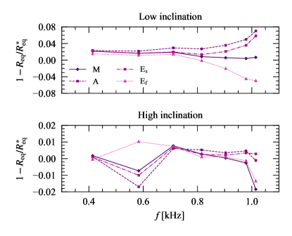
Figure 10: Fractional difference between injected $R_{\rm eq}^{\ast}$ and inferred best fit equatorial radii $R_{\rm eq}$ as a function of the rotation frequency $f$ for the different fitting formulas. For the low-inclination orientation the error stays below 10%, with the “fast” elliptic fit recovering the injected $R_{\rm eq}$ at high frequencies. For the high-inclination orientation all formulas recover the injected $R_{\rm eq}$ with less than 2% precision independently of $f$. In both cases panels, all fractional errors are smaller than the statistical errors we have assumed (0.2 for the low inclination and 0.05 for the high inclination scenarios).

Model	$R^{\ast}_{\rm eq}$	$f$	$R_{\rm eq}^{\rm M}$	$R_{\rm eq}^{\rm A}$	$R_{\rm eq}^{{\rm E}_{\rm s}}$	$R_{\rm eq}^{{\rm E}_{\rm f}}$
	(km)	(Hz)	(km)	(km)	(km)	(km)
1	12.00	413.8	($11.74^{+1.73}_{-1.48}$) $11.98^{+0.50}_{-0.49}$	($11.72^{+1.72}_{-1.46}$) $11.99^{+0.50}_{-0.49}$	($11.74^{+1.73}_{-1.47}$) $11.99^{+0.50}_{-0.49}$	($11.82^{+1.73}_{-1.47}$) $12.01^{+0.51}_{-0.50}$
2	12.27	583.4	($12.07^{+1.58}_{-1.39}$) $12.36^{+0.36}_{-0.40}$	($12.00^{+1.55}_{-1.34}$) $12.48^{+0.38}_{-0.38}$	($12.07^{+1.58}_{-1.39}$) $12.39^{+0.37}_{-0.39}$	($12.13^{+1.57}_{-1.38}$) $12.15^{+0.35}_{-0.40}$
3	12.57	710.9	($12.42^{+1.43}_{-1.31}$) $12.56^{+0.49}_{-0.48}$	($12.29^{+1.37}_{-1.22}$) $12.58^{+0.50}_{-0.48}$	($12.41^{+1.43}_{-1.29}$) $12.57^{+0.48}_{-0.49}$	($12.48^{+1.42}_{-1.32}$) $12.56^{+0.72}_{-0.49}$
4	12.90	815.4	($12.79^{+1.28}_{-1.25}$) $12.86^{+0.45}_{-0.47}$	($12.55^{+1.17}_{-1.08}$) $12.83^{+0.47}_{-0.48}$	($12.73^{+1.25}_{-1.16}$) $12.87^{+0.45}_{-0.46}$	($12.92^{+1.30}_{-1.37}$) $12.89^{+0.44}_{-0.45}$
5	13.27	903.7	($13.20^{+1.13}_{-1.22}$) $12.27^{+0.52}_{-0.53}$	($12.80^{+0.98}_{-0.92}$) $13.23^{+0.51}_{-0.51}$	($13.00^{+1.05}_{-0.97}$) $13.25^{+0.51}_{-0.51}$	($13.54^{+1.30}_{-1.66}$) $13.26^{+0.52}_{-0.50}$
6	13.70	978.9	($13.64^{+1.02}_{-1.24}$) $13.73^{+0.50}_{-0.53}$	($13.01^{+0.79}_{-0.76}$) $13.63^{+0.49}_{-0.52}$	($13.21^{+0.83}_{-0.76}$) $13.65^{+0.48}_{-0.50}$	($14.31^{+1.46}_{-1.77}$) $13.72^{+0.44}_{-0.48}$
7	14.19	1041.7	($14.09^{+0.94}_{-1.22}$) $14.45^{+0.37}_{-0.62}$	($13.20^{+0.60}_{-0.59}$) $14.20^{+0.37}_{-0.55}$	($13.36^{+0.61}_{-0.55}$) $14.15^{+0.30}_{-0.51}$	($14.89^{+1.47}_{-1.24}$) $14.38^{+0.21}_{-0.45}$

Table 7: Inferred equatorial radii $R_{\rm eq}$ for each fitting formula. The first three columns correspond to the benchmark star label, its equatorial radius and its rotation frequency, respectively. The remaining columns are the median and the $\pm 1\sigma$ credible intervals as inferred by using the different fitting formulas in the pulse profile model. For the inferred $R_{\rm eq}$ entries, the results between parenthesis correspond to the low-orientation case, while the others to the high-inclination case.

Model	$R^{\ast}_{\rm eq}$	$f$	$R_{\rm eq}^{\rm M}$ as in Morsink et al. (2007)	$R_{\rm eq}^{\rm A}$ as in AlGendy and Morsink (2014)
	(km)	(Hz)	(km)	(km)
1	12.00	413.8	($11.72^{+1.72}_{-1.47}$) $11.96^{+0.49}_{-0.48}$	($11.74^{+1.73}_{-1.47}$) $11.99^{+0.50}_{-0.49}$
2	12.27	583.4	($12.02^{+1.56}_{-1.37}$) $12.44^{+0.38}_{-0.39}$	($12.04^{+1.56}_{-1.37}$) $12.38^{+0.37}_{-0.39}$
3	12.57	710.9	($12.34^{+1.40}_{-1.30}$) $12.55^{+0.50}_{-0.48}$	($12.35^{+1.39}_{-1.25}$) $12.57^{+0.48}_{-0.49}$
4	12.90	815.4	($12.67^{+1.25}_{-1.21}$) $12.82^{+0.47}_{-0.49}$	($12.65^{+1.21}_{-1.13}$) $12.86^{+0.45}_{-0.47}$
5	13.27	903.7	($13.02^{+1.10}_{-1.15}$) $12.24^{+0.53}_{-0.54}$	($12.94^{+1.04}_{-0.98}$) $13.24^{+0.52}_{-0.50}$
6	13.70	978.9	($13.38^{+0.96}_{-1.11}$) $13.72^{+0.52}_{-0.57}$	($13.20^{+0.84}_{-0.84}$) $13.66^{+0.50}_{-0.51}$
7	14.19	1041.7	($13.73^{+0.84}_{-1.06}$) $14.45^{+0.47}_{-0.64}$	($13.42^{+0.66}_{-0.66}$) $14.26^{+0.36}_{-0.56}$

Table 8: Inferred equatorial radii $R_{\rm eq}$ using the formulas of Morsink et al.  Morsink et al. (2007) and AlGendy & Morsink  AlGendy and Morsink (2014), and the fitting coefficients obtained originally in these works. The table is analogous to Table 7. Overall, the relative difference ($\equiv 2\cdot|a-b|/|a+b|$) between the median values of $R_{\rm eq}$ using our and the original fitting coefficients is below 3%. Among both formulas, the largest fractional difference between best-fit $R_{\rm eq}$ and the injected $R_{\rm eq}^{\ast}$ values happens for the AlGendy & Morsink formula (7.6%, Model 7).

IV Conclusions

We studied the systematic error introduced by the use of analytical formulas to describe the surface of rapidly rotating neutron stars. These formulas are constructed by fitting certain analytical expressions to an ensemble of neutron star models described by a variety of equations of state and covering a wide range of compactness and spin parameter values. Neutron stars, however, are believed to be described by a single equation of state, and therefore, the fitting procedure used to obtain these surface formulas introduces a source of systematic error in the parameter estimation of neutron star properties, which could have implications to x-ray pulse profile observations with NICER.

To study the impact of this systematic error, we performed a restricted likelihood analysis using synthetic pulse profile data. We found that the systematic error described above is smaller than the statistical error indicating, albeit in a simplified analysis, that the radius parameter estimation by NICER Riley et al. (2019); Miller et al. (2019a) is not affected by it. It would be interesting to repeat the analysis carried here in a complete set-up following, for instance, the theoretical studies in Lo et al. (2013, 2018); Miller (2016), using as the injection pulse profile (i.e. synthetic signal) one calculated using the “exact” formulas obtained here. More specifically, it would be interesting to investigate the cumulative effect of this systematic error when one considers multiple finite-sized hot spots Sotani et al. (2019); Sotani (2020) and how it depends on their location on the star’s surface. As seen in Fig. 6 this error has a nontrivial behavior in the case of a single, pointlike hot spot. It would be important to analyze it in more realistic hot spot geometries ideally reproducing the hot spot configurations as inferred by NICER for PSR J0030+0451 Riley et al. (2019); Miller et al. (2019a). We think it is unlikely that this systematic error will matter for the slowly-spinning neutron stars targeted by NICER, but we hope our work motivates further studies, which should also include the level of realism of a full statistical analysis as done in Riley et al. (2019); Miller et al. (2019a).

Another interesting question to explore is how our ignorance on the equation of state affects the resulting fitting formulas. In our analysis, we used for our synthetic data the pulse profile emitted from the surface of a neutron star whose equation of state was also used to obtained the fitting formulas. In practice, it is unlikely that this situation will happen and it would then be important to investigate the variability (and the implications to radii inferences) of using different equation of state catalogs which could differ from the one used here to produce the surface fits.

Finally, it would also be important to repeat this analysis in the context of future large-area x-ray timing facilities Watts et al. (2019), such as the enhanced X-ray Timing and Polarimetry (eXTP) Zhang et al. (2019) and the Spectroscopic Time-Resolving Observatory for Broadband Energy X-rays (STROBE-X) Ray et al. (2018, 2019) missions. These future missions are expected to provide more precise parameter estimation of the radii of neutron stars relative to NICER’s current capabilities. As the statistical error is decreased, all sources of systematic errors will become more important, and the one discussed here may be of relevance.

As by-products of our study we also presented a method to accurately locate the surface of rotating neutron star solutions obtained with RNS. An implementation of the method is publicly available in Pappas . Moreover, we have also introduced a new analytical formula to describe the surface of rapidly rotating neutron stars. This formula, based on the ellipsoidal isodensity approximation Lai et al. (1993), better captures the surface of rapidly rotating neutron stars relative to other formulas known in the literature. The application range of this new formula is not limited by the problems studied here, and it could also be used to model the effect of stellar oblateness on parameter estimation using the cooling tail method Suleimanov et al. (2020) or in the wave propagation on thin oceans on neutron star surfaces van Baal et al. (2020).

Appendix A “Exact” surfaces: numerical derivatives, error estimates, and fits

In this appendix we show the details behind the fits for the star surface $R$ and its logarithmic-derivative ${\rm d}\log R/{\rm d}\theta$ used to model the shape of our benchmark stars.

First, to assess the numerical error associated with the surface data $R$ we computed neutron star solutions with two different resolutions using the RNS code.

The RNS code solves for the neutron star model’s interior and exterior on a grid with the radial coordinate $r$ compactified and equally spaced in the interval $s\in[0,1]$, using the definition $s\equiv r/(r+r_{\rm eq})$, and the angular coordinate $\mu=\cos\theta$ also equally spaced in the interval $\mu\in[0,1]$. This way, the code assigns half of the grid to the interior of the star (the equatorial location of the surface is always at $s=1/2$) and the other half to the vacuum exterior. The radial resolution near the surface, if we assume that we have chosen $S$ grid points, will be

$$\Delta r|_{r_{\rm eq}}\sim r_{\rm eq}\left(\frac{4}{2+S}\right)\,,$$ (35)

which for a star with $r_{\rm eq}$ approximately 10 km and grid sizes of $S=301$ and $S=1201$ points is around $0.13$ and $0.033$ km respectively. The usual choice for the angular grid is to be half of the radial one. Therefore in our calculations we have used both a low resolution grid of size $301\times 151$ points and a high resolution grid of size $1201\times 601$ points.

Once a neutron star solution is obtained, with either resolution, the star’s surface is obtained by the loci of the circumferential radius where the enthalpy per unit mass becomes equal to zero [see Eq. (2)].

To obtain an estimate on the numerical error on $R$ for our high-resolution solution ($\epsilon_{\rm high}$), we calculate the maximum fractional difference between the high-resolution and low-resolution solutions (evaluated at the same grid points $\mu_{i}$), namely

$$\epsilon_{\rm high}=\textrm{max}|1-R_{\rm low}(\mu_{i})/R_{\rm high}(\mu_{i})|\,.$$ (36)

We find that $\epsilon_{\rm high}$ is of the order of $10^{-5}$ for all stars in Table 1. We used the high-resolution data to obtain all fits.

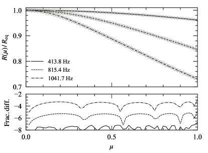
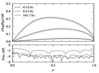
Figure 11: Surface and logarithmic-derivative of the three sample benchmark star models (with spin frequencies $f=413.8$, $815.4$, and $1041.7$ Hz) as functions of the colatitude $\theta$. In all panels, the markers correspond to the numerical data, whereas the lines to the fitting formulas (24). Left-top panel: the star’s surface normalized relative to its equatorial radius as a function of $\mu=\cos\theta$. Right-top panel: the star’s logarithmic-derivative relative to $\theta$ also as a function of $\mu$. Bottom panels: the fractional differences $\log_{10}|1-y_{\rm fit}/y_{\rm data}|$ between fit ($y_{\rm fit}$) and numerical data ($y_{\rm data}$).

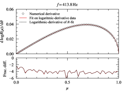
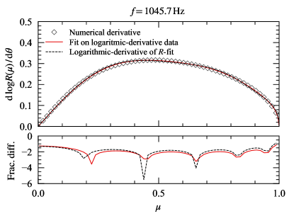
Figure 12: The logarithmic-derivative of the surface data. In the top panels the markers show the logarithmic derivative calculated using a sixth-order central finite difference scheme [Eq. (37)]. The dashed lines show the fits directly applied to this data using Eq. (24b) and the solid lines show the predicted logarithmic-derivative obtained by first applying Eq. (24a) to $R(\mu)$ and then taking the logarithmic-derivative. The fractional differences $\log_{10}|1-y_{\rm fit}/y_{\rm data}|$ between fit ($y_{\rm fit}$) and numerical data ($y_{\rm data}$) are shown in the bottom panels. The left panels corresponds to a star with spin frequency $f=413.8$ Hz, whereas the right panels corresponds to a star with spin frequency $f=1045.7$ Hz. For the slowest spinning case (left figure), both approaches agree well with the numerical data. However, for the fastest spinning case (right figure) the fractional differences are, except at a few points, slightly larger when using Eq. (24a). This fact justifies the use of a separate fit based on Eq. (24b) to model the surficial numerical derivatives.

In Fig. 11 we show the surface (left panel) and its logarithmic-derivative (right panel) as functions of $\mu=\cos\theta$ for three sample benchmark stars. We find that our fits (curves) agree with the numerical data (markers) within less then 1% fractional differences for all three cases.

In Fig. 12 we show the logarithmic derivative of the stellar surface as function of $\mu$ for the slowest (left panel) and the fastest (right panel) spinning benchmark star. In both panels the markers show the logarithmic derivative obtained by applying Eq. (37) to the high-resolution numerical data. The curves correspond to two approaches to model this data. More specifically, the solid curves correspond to fits obtained by directly applying Eq. (24b) to fit the data, while the dashed curves correspond to first fitting $R(\mu)$ using Eq. (24a) and then taking the logarithmic derivative. We see that both approaches agree very well for the $f=413.8$ Hz spinning star. However, for the $f=1045.7$ Hz spinning star, the former approach performs better overall, except at a few points. As a consequence, we used a separate fit based on Eq. (24b) to model the surficial numerical derivatives.

Let us now consider the logarithmic-derivative of $R$, defined in Eq. (22)

$$\frac{{\rm d}\log R(\mu)}{{\rm d}\theta}=-(1-\mu^{2})^{1/2}\frac{1}{R(\mu)}\frac{{\rm d}R(\mu)}{{\rm d}\mu}\,.$$

We calculate the derivative numerically using our high-resolution surface data and using a six-order central finite difference formula,

$$\frac{{\rm d}R}{{\rm d}\mu} =\left[R(\mu+3\Delta\mu)-9R(\mu+2\Delta\mu)+45R(\mu+\Delta\mu)\right.$$

$$\quad\left.-45R(\mu-\Delta\mu)+9R(\mu-2\Delta\mu)-R(\mu-3\Delta\mu)\right]$$

$$\quad\cdot(60\,\Delta\mu)^{-1}+{\cal O}(\Delta\mu^{6})\,,$$ (37)

where $\Delta\mu$ (the $\mu$-grid size) is approximately $1.67\cdot 10^{-3}$.

We quantify the error on the numerical derivative by doing the calculation at two different resolutions $\Delta\mu$ and $2\Delta\mu$. Using Eq. (36), we find that the error using the finer grid varies between approximately $5\cdot 10^{-4}$ for the fastest rotating star and $7\cdot 10^{-3}$ for the slowest rotating star.

References

- Lattimer and Prakash (2007) J. M. Lattimer and M. Prakash, Phys. Rept. 442, 109 (2007), arXiv:astro-ph/0612440 .
- Baym et al. (2018) G. Baym, T. Hatsuda, T. Kojo, P. D. Powell, Y. Song, and T. Takatsuka, Rept. Prog. Phys. 81, 056902 (2018), arXiv:1707.04966 [astro-ph.HE] .
- Özel (2013) F. Özel, Rept. Prog. Phys. 76, 016901 (2013), arXiv:1210.0916 [astro-ph.HE] .
- Miller and Lamb (2016) M. C. Miller and F. K. Lamb, Eur. Phys. J. A 52, 63 (2016), arXiv:1604.03894 [astro-ph.HE] .
- Degenaar and Suleimanov (2018) N. Degenaar and V. F. Suleimanov, Astrophys. Space Sci. Libr. 457, 185 (2018), arXiv:1806.02833 [astro-ph.HE] .
- Gendreau et al. (2012) K. C. Gendreau, Z. Arzoumanian, and T. Okajima, in Space Telescopes and Instrumentation 2012: Ultraviolet to Gamma Ray, Proc. SPIE, Vol. 8443 (2012) p. 844313.
- Arzoumanian et al. (2014) Z. Arzoumanian et al., in Space Telescopes and Instrumentation 2014: Ultraviolet to Gamma Ray, Proc. SPIE, Vol. 9144 (2014) p. 914420.
- Gendreau and Arzoumanian (2017) K. Gendreau and Z. Arzoumanian, Nature Astronomy 1, 895 (2017).
- Watts et al. (2016) A. L. Watts et al., Rev. Mod. Phys. 88, 021001 (2016), arXiv:1602.01081 [astro-ph.HE] .
- Watts (2019) A. L. Watts, AIP Conf. Proc. 2127, 020008 (2019), arXiv:1904.07012 [astro-ph.HE] .
- Riley et al. (2019) T. E. Riley et al., Astrophys. J. Lett. 887, L21 (2019), arXiv:1912.05702 [astro-ph.HE] .
- Miller et al. (2019a) M. Miller et al., Astrophys. J. Lett. 887, L24 (2019a), arXiv:1912.05705 [astro-ph.HE] .
- Silva et al. (2020) H. O. Silva, A. M. Holgado, A. Cárdenas-Avendaño, and N. Yunes, (2020), arXiv:2004.01253 [gr-qc] .
- Bogdanov et al. (2019a) S. Bogdanov et al., Astrophys. J. Lett. 887, L25 (2019a), arXiv:1912.05706 [astro-ph.HE] .
- Raithel (2019) C. A. Raithel, Eur. Phys. J. A 55, 80 (2019), arXiv:1904.10002 [astro-ph.HE] .
- Raaijmakers et al. (2019) G. Raaijmakers et al., Astrophys. J. Lett. 887, L22 (2019), arXiv:1912.05703 [astro-ph.HE] .
- Raaijmakers et al. (2020) G. Raaijmakers et al., Astrophys. J. Lett. 893, L21 (2020), arXiv:1912.11031 [astro-ph.HE] .
- Jiang et al. (2020) J.-L. Jiang, S.-P. Tang, Y.-Z. Wang, Y.-Z. Fan, and D.-M. Wei, Astrophys. J. 892, 1 (2020), arXiv:1912.07467 [astro-ph.HE] .
- Zimmerman et al. (2020) J. Zimmerman, Z. Carson, K. Schumacher, A. W. Steiner, and K. Yagi, (2020), arXiv:2002.03210 [astro-ph.HE] .
- Dietrich et al. (2020) T. Dietrich, M. W. Coughlin, P. T. H. Pang, M. Bulla, J. Heinzel, L. Issa, I. Tews, and S. Antier, Science 370, 1450 (2020), arXiv:2002.11355 [astro-ph.HE] .
- Chatziioannou (2020) K. Chatziioannou, Gen. Rel. Grav. 52, 109 (2020), arXiv:2006.03168 [gr-qc] .
- Essick et al. (2020) R. Essick, I. Tews, P. Landry, S. Reddy, and D. E. Holz, Phys. Rev. C 102, 055803 (2020), arXiv:2004.07744 [astro-ph.HE] .
- Cadeau et al. (2005) C. Cadeau, D. A. Leahy, and S. M. Morsink, Astrophys. J. 618, 451 (2005), arXiv:astro-ph/0409261 .
- Cadeau et al. (2007) C. Cadeau, S. M. Morsink, D. Leahy, and S. S. Campbell, Astrophys. J. 654, 458 (2007), arXiv:astro-ph/0609325 .
- Morsink et al. (2007) S. M. Morsink, D. A. Leahy, C. Cadeau, and J. Braga, Astrophys. J. 663, 1244 (2007), arXiv:astro-ph/0703123 [astro-ph] .
- Bogdanov et al. (2019b) S. Bogdanov et al., Astrophys. J. Lett. 887, L26 (2019b), arXiv:1912.05707 [astro-ph.HE] .
- Miller and Lamb (1998) M. C. Miller and F. K. Lamb, Astrophys. J. 499, L37 (1998), arXiv:astro-ph/9711325 [astro-ph] .
- Poutanen and Gierlinski (2003) J. Poutanen and M. Gierlinski, Mon. Not. Roy. Astron. Soc. 343, 1301 (2003), arXiv:astro-ph/0303084 .
- Poutanen and Beloborodov (2006) J. Poutanen and A. M. Beloborodov, Mon. Not. Roy. Astron. Soc. 373, 836 (2006), arXiv:astro-ph/0608663 [astro-ph] .
- Paschalidis and Stergioulas (2017) V. Paschalidis and N. Stergioulas, Living Rev. Rel. 20, 7 (2017), arXiv:1612.03050 [astro-ph.HE] .
- AlGendy and Morsink (2014) M. AlGendy and S. M. Morsink, Astrophys. J. 791, 78 (2014), arXiv:1404.0609 [astro-ph.HE] .
- Stergioulas and Friedman (1995) N. Stergioulas and J. Friedman, Astrophys. J. 444, 306 (1995), arXiv:astro-ph/9411032 [astro-ph] .
- Komatsu et al. (1989a) H. Komatsu, Y. Eriguchi, and I. Hachisu, Mon. Not. Roy. Astron. Soc. 237, 355 (1989a).
- Komatsu et al. (1989b) H. Komatsu, Y. Eriguchi, and I. Hachisu, Mon. Not. Roy. Astron. Soc. 239, 153 (1989b).
- Cook et al. (1994a) G. B. Cook, S. L. Shapiro, and S. A. Teukolsky, Astrophys. J. 424, 823 (1994a).
- Cook et al. (1994b) G. B. Cook, S. L. Shapiro, and S. A. Teukolsky, Astrophys. J. 422, 227 (1994b).
- Baym et al. (1971) G. Baym, C. Pethick, and P. Sutherland, Astrophys. J. 170, 299 (1971).
- Lorenz et al. (1993) C. P. Lorenz, D. G. Ravenhall, and C. J. Pethick, Phys. Rev. Lett. 70, 379 (1993).
- Douchin and Haensel (2001) F. Douchin and P. Haensel, Astron. Astrophys. 380, 151 (2001), arXiv:astro-ph/0111092 [astro-ph] .
- Wiringa et al. (1988) R. B. Wiringa, V. Fiks, and A. Fabrocini, Phys. Rev. C 38, 1010 (1988).
- Negele and Vautherin (1973) J. W. Negele and D. Vautherin, Nucl. Phys. A 207, 298 (1973).
- Akmal et al. (1998) A. Akmal, V. R. Pandharipande, and D. G. Ravenhall, Phys. Rev. C 58, 1804 (1998), arXiv:nucl-th/9804027 [nucl-th] .
- Pandharipande et al. (1976) V. R. Pandharipande, D. Pines, and R. A. Smith, Astrophys. J. 208, 550 (1976).
- Abbott et al. (2018) B. P. Abbott et al. (LIGO Scientific, Virgo), Phys. Rev. Lett. 121, 161101 (2018), arXiv:1805.11581 [gr-qc] .
- Tolman (1939) R. C. Tolman, Phys. Rev. 55, 364 (1939).
- Oppenheimer and Volkoff (1939) J. Oppenheimer and G. Volkoff, Phys. Rev. 55, 374 (1939).
- Hessels et al. (2006) J. W. Hessels, S. M. Ransom, I. H. Stairs, P. C. C. Freire, V. M. Kaspi, and F. Camilo, Science 311, 1901 (2006), arXiv:astro-ph/0601337 .
- Miller et al. (2019b) M. C. Miller, F. K. Lamb, A. J. Dittmann, S. Bogdanov, Z. Arzoumanian, K. C. Gendreau, S. Guillot, A. K. Harding, W. C. G. Ho, J. M. Lattimer, R. M. Ludlam, S. Mahmoodifar, S. M. Morsink, P. S. Ray, T. E. Strohmayer, K. S. Wood, T. Enoto, R. Foster, T. Okajima, G. Prigozhin, and Y. Soong, “NICER PSR J0030+0451 Illinois-Maryland MCMC Samples,” (2019b).
- Lommen et al. (2000) A. N. Lommen, A. Zepka, D. C. Backer, M. McLaughlin, J. C. Cordes, Z. Arzoumanian, and K. Xilouris, Astrophys. J. 545, 1007 (2000), arXiv:astro-ph/0008054 .
- Arzoumanian et al. (2018a) Z. Arzoumanian et al. (NANOGrav), Astrophys. J. Suppl. 235, 37 (2018a), arXiv:1801.01837 [astro-ph.HE] .
- Hartle (1967) J. B. Hartle, Astrophys. J. 150, 1005 (1967).
- Hartle and Thorne (1968) J. B. Hartle and K. S. Thorne, Astrophys. J. 153, 807 (1968).
- Berti et al. (2005) E. Berti, F. White, A. Maniopoulou, and M. Bruni, Mon. Not. Roy. Astron. Soc. 358, 923 (2005), arXiv:gr-qc/0405146 .
- Friedman and Stergioulas (2013) J. L. Friedman and N. Stergioulas, Rotating Relativistic Stars, Cambridge Monographs on Mathematical Physics (Cambridge University Press, 2013).
- (55) G. Pappas, “The surface of rapidly-rotating neutron stars,” https://github.com/GPappasGR/rapidly_RNS_surfaces.
- Suleimanov et al. (2017) V. F. Suleimanov, J. Poutanen, J. Nättilä, J. J. E. Kajava, M. G. Revnivtsev, and K. Werner, Mon. Not. Roy. Astron. Soc. 466, 906 (2017), arXiv:1611.09885 [astro-ph.HE] .
- Suleimanov et al. (2020) V. F. Suleimanov, J. Poutanen, and K. Werner, Astron. Astrophys. 639, A33 (2020), arXiv:2005.09759 [astro-ph.HE] .
- Yagi and Yunes (2017) K. Yagi and N. Yunes, Phys. Rept. 681, 1 (2017), arXiv:1608.02582 [gr-qc] .
- Benhar et al. (2005) O. Benhar, V. Ferrari, L. Gualtieri, and S. Marassi, Phys. Rev. D 72, 044028 (2005), arXiv:gr-qc/0504068 .
- Yagi et al. (2014) K. Yagi, K. Kyutoku, G. Pappas, N. Yunes, and T. A. Apostolatos, Phys. Rev. D 89, 124013 (2014), arXiv:1403.6243 [gr-qc] .
- Psaltis and Özel (2014) D. Psaltis and F. Özel, Astrophys. J. 792, 87 (2014), arXiv:1305.6615 [astro-ph.HE] .
- Oliva-Mercado and Frutos-Alfaro (2020) G. A. Oliva-Mercado and F. Frutos-Alfaro, (2020), arXiv:2006.05948 [gr-qc] .
- Lai et al. (1993) D. Lai, F. A. Rasio, and S. L. Shapiro, Astrophys. J. Suppl. 88, 205 (1993).
- Stein et al. (2014) L. C. Stein, K. Yagi, and N. Yunes, Astrophys. J. 788, 15 (2014), arXiv:1312.4532 [gr-qc] .
- Ransom et al. (2011) S. Ransom et al., Astrophys. J. Lett. 727, L16 (2011), arXiv:1012.2862 [astro-ph.HE] .
- Demorest et al. (2010) P. Demorest, T. Pennucci, S. Ransom, M. Roberts, and J. Hessels, Nature 467, 1081 (2010), arXiv:1010.5788 [astro-ph.HE] .
- Fonseca et al. (2016) E. Fonseca et al., Astrophys. J. 832, 167 (2016), arXiv:1603.00545 [astro-ph.HE] .
- Arzoumanian et al. (2018b) Z. Arzoumanian et al. (NANOGRAV), Astrophys. J. 859, 47 (2018b), arXiv:1801.02617 [astro-ph.HE] .
- Antoniadis et al. (2013) J. Antoniadis et al., Science 340, 6131 (2013), arXiv:1304.6875 [astro-ph.HE] .
- Cromartie et al. (2019) H. T. Cromartie et al., Nat. Astron. 4, 72 (2019), arXiv:1904.06759 [astro-ph.HE] .
- Abbott et al. (2017) B. Abbott et al. (LIGO Scientific, Virgo), Phys. Rev. Lett. 119, 161101 (2017), arXiv:1710.05832 [gr-qc] .
- Abbott et al. (2019) B. Abbott et al. (LIGO Scientific, Virgo), Phys. Rev. X 9, 011001 (2019), arXiv:1805.11579 [gr-qc] .
- Salmi et al. (2018) T. Salmi, J. Nättilä, and J. Poutanen, Astron. Astrophys. 618, A161 (2018), arXiv:1805.01149 [astro-ph.HE] .
- Lo et al. (2013) K. H. Lo, M. C. Miller, S. Bhattacharyya, and F. K. Lamb, Astrophys. J. 776, 19 (2013), arXiv:1304.2330 [astro-ph.HE] .
- Lo et al. (2018) K. H. Lo, M. C. Miller, S. Bhattacharyya, and F. K. Lamb, Astrophys. J. 854, 187 (2018), arXiv:1801.08031 [astro-ph.HE] .
- Miller (2016) M. C. Miller, Astrophys. J. 822, 27 (2016), arXiv:1602.00312 [astro-ph.HE] .
- Silva and Yunes (2019) H. O. Silva and N. Yunes, Class. Quant. Grav. 36, 17LT01 (2019), arXiv:1902.10269 [gr-qc] .
- Ayzenberg et al. (2016) D. Ayzenberg, K. Yagi, and N. Yunes, Class. Quant. Grav. 33, 105006 (2016), arXiv:1601.06088 [astro-ph.HE] .
- Ayzenberg and Yunes (2017) D. Ayzenberg and N. Yunes, Class. Quant. Grav. 34, 115003 (2017), arXiv:1701.07003 [gr-qc] .
- Sotani et al. (2019) H. Sotani, H. O. Silva, and G. Pappas, Phys. Rev. D 100, 043006 (2019), arXiv:1905.07668 [astro-ph.HE] .
- Sotani (2020) H. Sotani, Phys. Rev. D 101, 063013 (2020), arXiv:2002.11840 [astro-ph.HE] .
- Watts et al. (2019) A. L. Watts et al., Sci. China Phys. Mech. Astron. 62, 29503 (2019).
- Zhang et al. (2019) S.-N. Zhang et al. (eXTP), Sci. China Phys. Mech. Astron. 62, 29502 (2019), arXiv:1812.04020 [astro-ph.IM] .
- Ray et al. (2018) P. S. Ray et al., Proc. SPIE Int. Soc. Opt. Eng. 10699, 1069919 (2018), arXiv:1807.01179 [astro-ph.IM] .
- Ray et al. (2019) P. S. Ray et al. (STROBE-X Science Working Group), (2019), arXiv:1903.03035 [astro-ph.IM] .
- van Baal et al. (2020) B. F. van Baal, F. R. Chambers, and A. L. Watts, Mon. Not. Roy. Astron. Soc. 496, 2098 (2020), arXiv:2006.06382 [astro-ph.HE] .