On the interaction of species capable of explosive growth

Abstract

In the classical Lotka-Volterra population models, the interacting species affect each other’s growth rate. We propose an alternative model, in which the species affect each other through the limitation coefficients, rather then through the growth rates. This appears to be more realistic: the presence of foxes is not likely to diminish the fertility of rabbits, but will contribute to limiting rabbit’s population. Both the cases of predation and of competition are considered, as well as competition in case of periodic coefficients. Our model becomes linear when one switches to the reciprocals of the variables. In another direction we use a similar idea to derive a multiplicity result for a class of periodic equations.

Key words: Explosive growth, predator-prey, competing species.

AMS subject classification: 34C11, 34C25, 92D25.

1 Introduction

One way of solving the logistic population equation (here $x=x(t)$)

(1.1) $$x^{\prime}=ax-bx^{2}$$

is to divide this equation by $x^{2}$, and obtain a linear equation for $u=\frac{1}{x}$. Here $a>0$ is the growth rate, and $b>0$ is the limitation (or self-limitation) coefficient, both given numbers. We wish to explore the interactions of two species with populations $x=x(t)$ and $y=y(t)$ for which the substitution $u=\frac{1}{x}$ and $v=\frac{1}{y}$ leads to a linear system. The model we consider is

(1.2) $$x^{\prime}=ax+x^{2}\left(\frac{b}{y}+e\right)$$

$$y^{\prime}=dy+y^{2}\left(\frac{c}{x}+f\right)\,,$$

with constants $a$,$b$,$c$,$d$,$e$ and $f$. Dividing the first equation by $x^{2}$, the second one by $y^{2}$, and setting $u=\frac{1}{x}$ and $v=\frac{1}{y}$, gives a linear system

(1.3) $$-u^{\prime}=au+bv+e$$

$$-v^{\prime}=cu+dv+f\,.$$

The signs of the coefficients determine the type of interaction, which will include both predator-prey and competing species cases.

Let us compare (1.2) with the classical Lotka-Volterra predator-prey model

(1.4) $$x^{\prime}=x\left(a-b\,y\right)$$

$$y^{\prime}=y\left(-c+d\,x\right)\,,$$

where the constants $a$,$b$,$c$,$d$ are positive. In (1.4) the species affect each other through the growth rate: the prey, with the number given by $x(t)$, improves the growth rate of the predator, with the number $y(t)$, while the predator decreases the growth rate of the prey. In the model (1.2) the species affect each other through their limitation coefficients. This appears to be more realistic: the presence of foxes is not likely to decrease the fertility of rabbits (new rabbits will be born at the same rate), but will place a limitation on the growth of rabbit population.

Similarly to the Lotka-Volterra model, the proposed model (1.2) predicts oscillatory behavior for predator-prey interaction, and either stable coexistence or competitive exclusion for competing species. Unlike the Lotka-Volterra model, it is possible that the population number of one of the species goes to infinity in finite time, while the number of the other species remains finite and positive. Explosive growth of populations occurs often in nature. Notice that our analysis leads to some non-standard questions about linear systems. For example, if a solution of (1.3) starts in the first quadrant of the $xy$-plane, will it stay in the first quadrant for all $t$?

Using the Floquet theory, we analyze a case of predator-prey interaction with periodic coefficients, and give a condition for the existence of a limit cycle.

In another direction we use the same transformation $u=\frac{1}{x}$ to derive a multiplicity result for a class of periodic equations

$$x^{\prime}(t)=f(t,x(t))\,,\;\;\;\;\mbox{with $f(t+p,x)=f(t,x)$}\,.$$

2 Explosive predator-prey model

Consider the model

(2.1) $$x^{\prime}=x^{2}\left(\frac{b}{y}-1\right)$$

$$y^{\prime}=-y^{2}\left(\frac{d}{x}-1\right)\,.$$

Here $x(t)$ gives the number of prey, and $y(t)$ the number of predator. If $y(t)$ is small, the prey grows explosively (with $x^{\prime}$ behaving like $\alpha x^{2}$, $\alpha>0$). If the number of predators $y(t)$ is large, then $x^{\prime}(t)<0$ and $x(t)$ decreases. The number of predators $y(t)$ decreases when $x(t)$ small, and grows explosively for $x(t)$ large. This model corresponds to (1.2), with $a=d=0$. The coefficients $e$ and $f$ have been scaled out.

The system (2.1) has a rest point $(d,b)$. Letting $X=\frac{\sqrt{d/b}}{x}$ and $Y=\frac{1}{y}$ transforms (2.1) into a perturbed harmonic oscillator

(2.2) $$X^{\prime}=-\sqrt{bd}\,Y+\sqrt{d/b}$$

$$Y^{\prime}=\sqrt{bd}\,X-1\,.$$

Setting $X(t)=\xi(t)+\frac{1}{\sqrt{bd}}$, $Y(t)=\eta(t)+\frac{1}{b}$ leads to a harmonic oscillator

$$\xi^{\prime}=-\sqrt{bd}\,\eta$$

$$\eta^{\prime}=\sqrt{bd}\,\xi\,,$$

so that the solution of (2.2) is

(2.3) $$X(t)=\frac{1}{\sqrt{bd}}+c_{1}\cos\sqrt{bd}\,t-c_{2}\sin\sqrt{bd}\,t$$

$$Y(t)=\frac{1}{b}+c_{1}\sin\sqrt{bd}\,t+c_{2}\cos\sqrt{bd}\,t\,,$$

which is just a rotation of the point $(X(0),Y(0))$ around the point $(\frac{1}{\sqrt{bd}},\frac{1}{b})$, the rest point of (2.2), on the circle of radius $\sqrt{c_{1}^{2}+c_{2}^{2}}$. The solution of (2.1) is then

(2.4) $$x(t)=\frac{\sqrt{d/b}}{\frac{1}{\sqrt{bd}}+c_{1}\cos\sqrt{bd}\,t-c_{2}\sin\sqrt{bd}\,t}$$

$$y(t)=\frac{1}{\frac{1}{b}+c_{1}\sin\sqrt{bd}\,t+c_{2}\cos\sqrt{bd}\,t}\,.$$

The constants $c_{1}$ and $c_{2}$ are determined from the initial values $(x(0),y(0))$:

(2.5) $$c_{1}=\frac{\sqrt{d/b}}{x(0)}-\frac{1}{\sqrt{bd}}\,,\;\;\mbox{ and}\;\;c_{2}=\frac{1}{y(0)}-\frac{1}{b}\,.$$

It is now clear that the rest point $(d,b)$ is a center for (2.1), and we can give a complete description of the behavior of positive solutions.

Theorem 2.1

Given the initial point $(x(0),y(0))$, calculate $c_{1}$ and $c_{2}$ by (2.5), and $R=\sqrt{c_{1}^{2}+c_{2}^{2}}$. If the circle $C$ of radius $R$ around the point $(\frac{1}{\sqrt{bd}},\frac{1}{b})$ lies completely inside the first quadrant of the $(X,Y)$ plane, then the corresponding solution $(x(t),y(t))$ of (2.1) is a closed curve around the rest point $(d,b)$, given by (2.4). Moreover, the period of all these closed curves is the same, and $x(t)>\frac{d}{2}$, $y(t)>\frac{b}{2}$ for all $t$. Assume now that this circle $C$, traveled counterclockwise beginning with the point $(X(0),Y(0))=(\frac{\sqrt{d/b}}{x(0)},\frac{1}{y(0)})$, hits one of the axes of the $(X,Y)$ plane. If it hits the $Y$-axis first, then there is a time $T>0$ so that $\lim_{t\rightarrow T}x(t)=\infty$, while $\lim_{t\rightarrow T}y(t)$ is finite and positive. If $C$ hits the $X$-axis first, then there is a time $T>0$ so that $\lim_{t\rightarrow T}y(t)=\infty$, while $\lim_{t\rightarrow T}x(t)$ is finite and positive.

Proof:    In view of the discussion above, it remains to prove the lower bounds for the periodic solutions in the first part of the theorem. From (2.3) one sees that the positivity of $X(t)$ and $Y(t)$ implies that $X(t)<\frac{2}{\sqrt{bd}}$ and $Y<\frac{2}{b}$, from which one gets the lower bounds on $x(t)$ and $y(t)$. $\diamondsuit$

Example Using Mathematica, we computed four periodic solutions for the system (2.1), with $b=3$ and $d=2$, surrounding the rest point at $(2,3)$, see Figure 1.

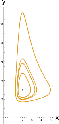
Figure 1: Periodic solutions for the system (2.1)

3 Explosive competing species model

Consider the model

(3.1) $$x^{\prime}=a\,x+x^{2}\left(\frac{b}{y}-1\right),\;\;x(0)>0$$

$$y^{\prime}=d\,y+y^{2}\left(\frac{c}{x}-1\right),\;\;y(0)>0\,,$$

with positive constants $a$,$b$,$c$ and $d$. Each species grows explosively, if the number of the other one is small, while if the competitor’s number is large, the growth is logistic-like. Clearly, the interaction is competitive in nature.

We begin with a simple observation: if $x(0)>0$ and $y(0)>0$, then $x(t)>0$ and $y(t)>0$ for all $t>0$. Indeed, writing the first equation in the form $x^{\prime}=A(t)x$, with $A(t)\equiv a+x(t)\left(\frac{b}{y(t)}-1\right)$, and integrating, obtain $x(t)=x(0)e^{\int_{0}^{t}A(s)\,ds}>0$. Similarly, $y(t)>0$ for all $t>0$. Hence, we can limit our study of (3.1) to the first quadrant of the $(x,y)$ plane.

Setting $X=\frac{1}{x}$ and $Y=\frac{1}{y}$ produces a linear system

(3.2) $$X^{\prime}=-aX-bY+1\,,\;\;X(0)=\frac{1}{x(0)}>0$$

$$Y^{\prime}=-cX-dY+1\,,\;\;Y(0)=\frac{1}{y(0)}>0\,,$$

with a unique rest point $(X_{0},Y_{0})$ given by

(3.3) $$X_{0}=\frac{d-b}{ad-bc}\,,\;\;Y_{0}=\frac{a-c}{ad-bc}\,.$$

Since $x(t)>0$ and $y(t)>0$ for all $t>0$, we may restrict the system (3.2) to the first quadrant of the $(X,Y)$ plane. The rest point $(X_{0},Y_{0})$ lies in the first quadrant if either

(3.4) $$d>b\;\mbox{ and}\;a>c\;\mbox{ (and then $ad>bc$)}\,,$$

or

(3.5) $$d<b\;\mbox{ and}\;a<c\;\mbox{ (and then $ad<bc$)}\,.$$

Letting $\xi=X-X_{0}$ and $\eta=Y-Y_{0}$, we translate the rest point to the origin, obtaining the system

(3.6) $$\xi^{\prime}=-a\xi-b\eta$$

$$\eta^{\prime}=-c\xi-d\eta\,,$$

with the matrix $A=\left[\begin{array}[]{rr}-a&-b\\ -c&-d\end{array}\right]$. The eigenvalues of $A$ are

$$\lambda_{1,2}=\frac{1}{2}\left(-a-d\pm\sqrt{a^{2}-2ad+4bc+d^{2}}\right)\,.$$

The corresponding (column) eigenvectors are

$$\xi_{1,2}=\left(-\frac{-a+d\pm\sqrt{a^{2}-2ad+4bc+d^{2}}}{2c},1\right)^{T}\,.$$

In case (3.4) holds, both eigenvalues are negative, and the rest point $(X_{0},Y_{0})$ is a stable node, while in case (3.5) holds, one eigenvalue is negative and the other one is positive, so that $(X_{0},Y_{0})$ is a saddle.

Theorem 3.1

(i) Assume that the condition (3.5) holds. Then one of the species (depending on the initial conditions) grows explosively. Namely, for any solution of (3.1) there is a time $T>0$ so that $\lim_{t\rightarrow T}x(t)=\infty$, while $\lim_{t\rightarrow T}y(t)$ is finite and positive, or the other way around.

(ii) Assume that the condition (3.4) holds. If $x(t)$ and $y(t)$ remain finite for all $t>0$ then $\lim_{t\rightarrow\infty}x(t)=\frac{1}{X_{0}}$ and $\lim_{t\rightarrow\infty}y(t)=\frac{1}{Y_{0}}$.

Proof:    The general solution of (3.2) is

(3.7) $$\left(X(t),Y(t)\right)^{T}=\left(X_{0},Y_{0}\right)^{T}+c_{1}e^{\lambda_{1}t}\xi_{1}+c_{2}e^{\lambda_{2}t}\xi_{2}\,.$$

(i) In case (3.5) holds, the eigenvalues of $A$ are of opposite sign say $\lambda_{1}<0<\lambda_{2}$. The term $c_{1}e^{\lambda_{1}t}\xi_{1}$ is negligible in the long run. The eigenvector $\xi_{2}$ corresponding to the positive eigenvalue (“plus” in front of the square root) has one component positive, and the other one is negative. It follows that all of the solutions of (3.2) eventually move either northwest or southeast of the rest point $(X_{0},Y_{0})$ intersecting either the $X$ or the $Y$ axis.

(ii) In case (3.4) holds, the general solution of (3.2) is given by (3.7), with negative $\lambda_{1}$ and $\lambda_{2}$. It follows that the point $\left(X(t),Y(t)\right)$ tends to the point $\left(X_{0}>0,Y_{0}>0\right)$ as $t\rightarrow\infty$. If the point $\left(X(t),Y(t)\right)$ stays in the first quadrant, then $x(t)$ and $y(t)$ are defined for all $t$, otherwise one of the species becomes infinite in finite time. $\diamondsuit$

Remark   In case (3.4) holds, the solution of (3.2) connects the points $\left(X_{0},Y_{0}\right)$ and $\left(X(0),Y(0)\right)$ in the first quadrant. While it is rare for the solution $\left(X(t),Y(t)\right)$ to exit the first quadrant, this may indeed happen if the points $\left(X_{0},Y_{0}\right)$ and $\left(X(0),Y(0)\right)$ lie near one of the axes. We used Mathematica to solve (3.2) with $a=4$, $b=1$, $c=1$, $d=5$, $X(0)=5$, $Y(0)=0.1$. Here $X_{0}=\frac{4}{19}>0$ and $Y_{0}=\frac{3}{19}>0$. The graph of the solution in Figure 2 shows that $Y(t)$ becomes zero at some $T$, which corresponds to $\lim_{t\rightarrow T}y(t)=\infty$.

Figure 2: A solution of the system (3.2) exiting the first quadrant of the $XY$-plane (the motion is from right to left)

4 Explosive predator-prey model with periodic coefficients

We now consider a periodic perturbation of the explosive predator-prey model

(4.1) $$x^{\prime}=x^{2}\left(\frac{b+\beta(t)}{y}-1\right)$$

$$y^{\prime}=-y^{2}\left(\frac{d+\delta(t)}{x}-1\right)\,,$$

with small continuous functions $\beta(t)$ and $\delta(t)$ of period $p$, so that $\beta(t+p)=\beta(t)$ and $\delta(t+p)=\delta(t)$ for all $t$. (We make no assumptions on the sign of $\beta(t)$ and $\delta(t)$.) The linear system for $X=\frac{1}{x}$ and $Y=\frac{1}{y}$

(4.2) $$X^{\prime}=-\left(b+\beta(t)\right)Y+1$$

$$Y^{\prime}=\left(d+\delta(t)\right)X-1$$

has $p$-periodic coefficients. Let $F(t)$ be the normalized fundamental solution matrix (with $F(0)=I$, the identity matrix) of the corresponding homogeneous system

(4.3) $$X^{\prime}=-\left(b+\beta(t)\right)Y$$

$$Y^{\prime}=\left(d+\delta(t)\right)X\,.$$

For small $\beta(t)$ and $\delta(t)$, $F(t)$ is close for $t\in[0,p]$ to the normalized fundamental solution matrix $F_{0}(t)=\left[\begin{array}[]{rr}\cos\sqrt{bd}\,t&-\sqrt{\frac{b}{d}}\sin\sqrt{bd}\,t\\ \sqrt{\frac{d}{b}}\sin\sqrt{bd}\,t&\cos\sqrt{bd}\,t\end{array}\right]$ of the unperturbed system

(4.4) $$X^{\prime}=-bY$$

$$Y^{\prime}=dX\,.$$

By the continuous dependence of eigenvalues on the coefficients of the matrix, the Floquet multipliers of (4.3), i.e., the eigenvalues of $F(p)$ are close to the eigenvalues $\rho_{1}$ and $\rho_{2}$ of $F_{0}(p)$. Clearly,

(4.5) $$\rho_{1}\rho_{2}=1=\det F_{0}(p)$$

$$\rho_{1}+\rho_{2}=2\cos\sqrt{bd}\,p={\rm trace}\,F_{0}(p)\,.$$

Theorem 4.1

Assume that $\sqrt{bd}\,p\neq 2\pi m$, for any integer $m$. Then the system (4.1) has a unique positive $p$-periodic solution $(x_{p}(t),y_{p}(t))$ for sufficiently small $\beta(t)$ and $\delta(t)$.

Proof:    Observe that $\rho_{i}\neq 1$, for $i=1,2$. Indeed, if $\rho_{1}=1$, then from the first line in (4.5) $\rho_{2}=1$, giving a contradiction in the second line in (4.5), because $\cos\sqrt{bd}\,p\neq 1$. Since $\beta(t)$ and $\delta(t)$ are small, the Floquet multipliers of the homogeneous problem (4.3) are different from one, so that (4.3) has no $p$-periodic solution, and then by a standard result the non-homogeneous system (4.2) (and hence the original system (4.1)) has a unique $p$-periodic solution $(X_{p}(t),Y_{p}(t))$. It remains to show that $X_{p}(t)>0$ and $Y_{p}(t)>0$ for all $t$.

We derive next an a priori bound on $X_{p}(t)$ and $Y_{p}(t)$, uniform in $\beta(t)$ and $\delta(t)$, provided that $|\beta(t)|+|\delta(t)|\leq c_{0}$, for some constant $c_{0}$. Indeed, integrating both equations in (4.2) over $(0,t)$, with $t\in(0,p)$, taking absolute values and then adding the corresponding inequalities, obtain

(4.6) $$|X_{p}(t)|+|Y_{p}(t)|\leq a_{1}\int_{0}^{t}\left(|X_{p}(s)|+|Y_{p}(s)|\right)\,ds+a_{2}\,,$$

for some positive constants $a_{1}$ and $a_{2}$. The desired bound over $(0,p)$ follows by the Bellman-Gronwall lemma, see e.g., [2].

We claim that $X_{p}(t)>0$ and $Y_{p}(t)>0$ for all $t$. Setting $X_{p}(t)=\xi(t)+\frac{1}{d}$ and $Y_{p}(t)=\eta(t)+\frac{1}{b}$ in (4.2) obtain

(4.7) $$\xi^{\prime}=-b\,\eta-\beta(t)Y_{p}(t)$$

$$\eta^{\prime}=d\xi+\delta(t)X_{p}(t)\,.$$

Express

$$\left[\begin{array}[]{r}\xi(t)\\ \eta(t)\end{array}\right]=F_{0}(t)\left[\begin{array}[]{r}c_{1}\\ c_{2}\end{array}\right]+F_{0}(t)\int_{0}^{t}F_{0}^{-1}(s)f(s)\,ds\,,$$

with some constants $c_{1}$ and $c_{2}$, and $f(t)=\left[\begin{array}[]{r}-\beta(t)Y_{p}(t)\\ \delta(t)X_{p}(t)\end{array}\right]$. Since the vector $\left[\begin{array}[]{r}\xi(t)\\ \eta(t)\end{array}\right]$ has period $p$, and the fundamental solution matrix $F_{0}(t)$ has period $\frac{2\pi m}{\sqrt{bd}}\neq p$, it follows that $c_{1}=c_{2}=0$. The vector $f(t)$ is small by our assumptions, and the a priori estimate (4.6). Both matrices $F_{0}(t)$ and $F_{0}^{-1}(s)$ have bounded entries. Then the vector $\left[\begin{array}[]{r}\xi(t)\\ \eta(t)\end{array}\right]$ is small, so that the trajectory $(X_{p}(t),Y_{p}(t))$ remains near the point $\left(\frac{1}{d},\frac{1}{b}\right)$, and hence it stays in the first quadrant for all $t$. $\diamondsuit$

5 Multiplicity of solutions for a class of periodic equations

The transformation $u(t)=\frac{1}{x(t)}$ of the preceding sections turns out to be useful for a class of first order equations with periodic coefficients. V.A. Pliss [5] considered what he called the Abel equation:

(5.1) $$x^{\prime}(t)=a_{0}(t)x^{3}+a_{1}(t)x^{2}+a_{2}(t)x+a_{3}(t)\,.$$

Assuming that the given functions $a_{i}(t)$, $0\leq i\leq 3$, are of period $p$, and $a_{0}(t)$ is either positive or negative for all $t$, he proved that the equation (5.1) has at most three $p$-periodic solutions. The proof involved a clever combination of the equations that the inverses of solutions satisfy.

What if one changes the $a_{0}(t)x^{3}$ term to $a_{0}(t)x^{2n+1}$? In case it is $a_{0}(t)x^{5}$, the method of V.A. Pliss [5] still gives the same result with a little extra effort. For higher powers things get more involved, and in fact existence of at most three $p$-periodic solutions was proved by another elegant method in A.A. Panov [4]. It turns out that the following more general result was already known.

Theorem 5.1

For the equation

(5.2) $$x^{\prime}(t)=f(t,x)$$

assume that the function $f(x,t)$ is continuous and has three continuous derivatives in $x$, and also for some $p>0$ and all real $t$ and $x$ one has

(5.3) $$f(t+p,x)=f(t,x)\,,$$

(5.4) $$f_{xxx}(t,x)>0\;\;\;\;\mbox{(or the opposite inequality holds)}\,.$$

Then the equation (5.2) has at most three $p$-periodic solutions.

This theorem follows from a more general result of A. Sandqvist and K.M. Andersen [6]. They considered the equation (5.2) on the interval $(0,p)$ and called a solution to be closed if $x(p)=x(0)$. Assuming the condition (5.4) holds, they showed that the problem (5.2) has at most three closed solutions, which implies the Theorem 5.1.

A simpler proof of the Theorem 5.1 was found in P. Korman and T. Ouyang [3]. We now simplify the presentation in that paper. The proof will follow from the following three simple lemmas.

Lemma 5.1

Assume the condition (5.4) holds and $f(t,0)=0$ for all $t\in R$. Then for all $t\in R$ and $x>0$ one has

$$Q(t,x)\equiv 2f(t,x)-2xf_{x}(t,x)+x^{2}f_{xx}(t,x)>0\,.$$

Proof:    Calculate $Q(t,0)=0$ and $Q_{x}(t,x)=x^{2}f_{xxx}(t,x)>0$. $\diamondsuit$

Lemma 5.2

For the problem

(5.5) $$y^{\prime}(t)=g(t,y)$$

assume that for some $p>0$ and all $t\in R$ and $y>0$ one has

$$g(t+p,y)=g(t,y)\,,$$

$$g_{yy}(t,y)>0\;\;\;\;\mbox{(or the opposite inequality holds)}\,.$$

Then the equation (5.5) has at most two positive $p$-periodic solutions.

The proof is standard, and it can be found in e.g., P. Korman [2], p. $245$. The next lemma is crucial.

Lemma 5.3

For the problem (5.2) assume that $f(t,0)=0$ for all $t\in R$, and the conditions (5.3),(5.4) hold for all $t\in R$ and $x>0$. Then the equation (5.2) has at most two positive $p$-periodic solutions.

Proof:    Set $x=\frac{1}{y}$ in (5.2). Then

(5.6) $$-y^{\prime}=y^{2}f(t,\frac{1}{y})\equiv g(t,y).$$

By Lemma 5.1 for any $y>0$

$$g_{yy}=2f(t,\frac{1}{y})-\frac{2}{y}f_{x}(t,\frac{1}{y})+\frac{1}{y^{2}}f_{xx}(t,\frac{1}{y})=2f(t,x)-2xf_{x}(t,x)+x^{2}f_{xx}(t,x)>0\,.$$

By Lemma 5.2 the equation (5.6) has at most two positive $p$-periodic solutions, and the same is true for (5.2). $\diamondsuit$

Turning to the proof of the Theorem 5.1, observe that different solutions of (5.2) do not intersect by the uniqueness theorem. If the equation (5.2) has four $p$-periodic solutions, let $\xi(t)$ be the smallest one. Then $z(t)=x(t)-\xi(t)$ satisfies

(5.7) $$z^{\prime}=f(t,z+\xi)-f(t,\xi)\equiv g(t,z)\,,$$

and the equation (5.7) has three positive $p$-periodic solutions. However, $g(t,0)=0$ and $g_{zzz}(t,z)>0$ for $z>0$, contradicting the Lemma 5.3.

Equations of the type (5.2) occur often in ecological problems, see e.g., S. Ahmad and A.C. Lazer [1], or P. Korman [2].

References

• [1] S. Ahmad and A.C. Lazer, Separated solutions of logistic equation with nonperiodic harvesting, J. Math. Anal. Appl. 445, no. 1, 710-718 (2017).
• [2] P. Korman, Lectures on Differential Equations, AMS/MAA Textbooks, Volume $54$, 2019.
• [3] P. Korman and T. Ouyang, Exact multiplicity results for two classes of periodic equations, J. Math. Anal. Appl. 194, no. 3, 763-779 (1995).
• [4] A.A. Panov, On the number of periodic solutions of polynomial differential equations. (Russian) Mat. Zametki 64, no. 5, 720-727 (1998); translation in Math. Notes, no. 5-6, 622-628 (1999).
• [5] V.A. Pliss, Nonlocal Problems of the Theory of Oscillations. Translated from the Russian by Scripta Technica, Inc. Academic Press, New York-London (1966).
• [6] A. Sandqvist and K.M. Andersen, On the number of closed solutions to an equation $x^{\prime}=f(t,x)$, where $f_{x^{n}}(t,x)\geq 0$ ($n=1$,$2$, or $3$), J. Math. Anal. Appl. 159, no. 1, 127-146 (1991).