Ultrasound Modulated Bioluminescence Tomography with a Single Optical Measurement
Abstract.
Ultrasound modulated bioluminescence tomography (UMBLT) is an imaging method which can be formulated as a hybrid inverse source problem. In the regime where light propagation is modeled by a radiative transfer equation, previous approaches to this problem require large numbers of optical measurements [10]. Here we propose an alternative solution for this inverse problem which requires only a single optical measurement in order to reconstruct the isotropic source. Specifically, we derive two inversion formulae based on Neumann series and Fredholm theory respectively, and prove their convergence under sufficient conditions. The resulting numerical algorithms are implemented and experimented to reconstruct both continuous and discontinuous sources in the presence of noise.
1. Introduction
BioLuminescence Tomography (BLT) is a technology that uses light emitted by optical probes to report activity at the molecular level. It has experienced rapid development in the past few decades due to its non-invasiveness and high optical contrast [17, 23]. However, BLT often suffers from low spatial resolution. This is because of the inherent ill-posedness of the inverse problem in BLT, where reconstruction of the internal distribution of bioluminescent molecules has to be implemented from data measured on the surface – see [9, 24] for more on this problem.
An effective approach to enhance the spatial resolution of BLT is by ultrasound modulation. This leads to the hybrid imaging modality known as Ultrasound Modulated BioLumnescence Tomography (UMBLT) [20, 11, 12, 10]. In UMBLT, typical BLT is performed while the optical properties of the object-of-interest undergoes a series of perturbation caused by acoustic vibrations. The inverse problem in UMBLT is to recover the spatial distribution of the optical probes from the perturbed boundary measurement of the emitted light. It turns out, as elucidated below, that the perturbed measurement allows retrieval of an internal functional, which helps mitigate the ill-posedness of the inverse problem and enhance the spatial resolution.
This basic idea, in which ultrasound modulation helps improve an otherwise ill-posed problem, has received quite a bit of recent theoretical attention in a number of different contexts. An early example is the problem of ultrasound modulated electrical impedance tomography discussed in [7]. In the context of optical tomography, in which one seeks to reconstruct coefficients instead of sources, see for example [2, 3, 4, 8, 16, 15]. Other related optical problems include fluorescent ultrasound modulated optical tomography ( [21, 22]) and multifrequency acousto-optic tomography ( [13, 14]). Ultrasound modulated hybrid problems are also part of a broader group of hybrid inverse problems in which the interactions of multiple imaging modalities create well-posed problems; for a survey of such ideas, see [6].
We turn to the mathematical formulation of the inverse problem in UMBLT. Let be a bounded open subset in with smooth boundary , . We model the propagation of light in the medium using the standard Radiative Transfer Equation (RTE):
| (1) |
Here represents the intensity of light at the point in the direction , is an isotropic source that is independent of , is the attenuation coefficient and is the scattering kernel. Let and be the outgoing boundary and the incoming boundary respectively, that is,
| (2) |
where is the unit outer normal vector at . Assume no light flows through the boundary so that the intensity obeys the boundary condition
| (3) |
Next, we take the effect of acoustic modulation into account. Suppose the incident acoustic wave is of the form where is the wave vector and is the phase. The time scale of the acoustic field propagation is generally much greater than that of the optical field, hence the acoustic field can effectively modulate the time independent RTE. In the presence of the acoustic modulation, the optical coefficients , , and the source become , , and , respectively. Following [11, 12], the effect of the acoustic modulation on the optical properties can be modeled as
| (4) | ||||
| (5) | ||||
| (6) |
where is the dimensionless amplitude of the pressure wave. The modulated RTE and boundary condition take the form
| (7) | ||||
| (8) |
where is the modulated RTE solution. We henceforth write for the RTE solution without modulation , that is, , the solution of the system (1), (3).
Under suitable assumptions on , and (see (A1)(A2) below), the boundary value problem (7) (8) admits a unique solution . The measurement is the operator defined as
| (9) |
This is the light that flows out through the boundary during various acoustic modulation
The inverse problem in UMBLT is to reconstruct the non-modulated source term from the operator , provided the non-modulated optical coefficients and are a-priori known.
Our contribution: The inverse problem of UMBLT was first studied in the special case of the diffusion approximation to the RTE [12]. It was shown that the source can be reconstructed with Lipschitz-type stability. The problem with full RTE model was later considered in [10], where uniqueness and stability results were established. These results are constructive and valid for general anisotropic sources. Nevertheless the reconstruction algorithm in [10] has serious drawbacks, stemming from the fact that it requires a point-by-point reconstruction in the interior of the domain. The reconstruction at each point requires a separate boundary integral to be calculated from boundary observations, which means in practice, and need to be known at each . This means precision relies on a huge volume of observations, and all of these observations need to be angularly resolved, which can be difficult to guarantee in practice. Moreover the precise boundary integral required for the reconstruction at a given point needs to be calculated by a process described in the proof of Theorem 1.3 of [10]. This requires repeated calculations of separate solutions to the RTE for every individual point of the domain, which in practice is extremely computationally demanding.
In contrast, the main result of the present paper is that under reasonable conditions (see Theorems 3 and 5 for precise statements), we can reconstruct an isotropic source from the knowledge of any single boundary integral of the form
where is the solution to the RTE (1) and is any uniformly positive continuous function on . This eliminates the requirement for multiple angularly resolved measurements on the boundary. Moreover it drastically reduces the computational demand, as demonstrated below.
The paper is structured as follows. In Section 2 we describe the derivation of an internal functional from the boundary data collected in the ultrasound modulated experiment, following the ideas of [10]. In Section 3, we present and discuss the main results, in which two inversion formulae are proved, one based on the Neumann series and the other on Fredholm inversion theory. Each of these formulae allows recovery of the isotropic source from measurement of a single boundary integral. Finally in Section 4, we describe numerical algorithms for implementing the ideas of Section 3, and present numerical results.
2. Derivation of the Internal Functional
Throughout the paper, we make the following assumptions to ensure well-posedness of some forward boundary value problems.
-
(A1):
and are continuous on
-
(A2):
Set , one of the following inequalities holds:
(10) where is a positive constant, or
(11) where is the diameter of .
In order to derive the internal functional, we make the additional assumption that is invariant under rotations, so
| (12) |
This ensures that the integral operator appearing in the RTE is self adjoint over .
Under the assumptions (A1) (A2), well-posedness of the RTE with a prescribed continuous incoming boundary condition and an anisotropic source is proved in [10, Theorem 2.1]. We will apply it to the special case (1) where the source is isotropic. In order to state the result, we define the norm ()
and the function space by
Proposition 1 ([10, Theorem 2.1]).
Here denotes the volume of . Note that for an isotropic source , .
Let be the solution to the following adjoint RTE with prescribed outgoing boundary condition :
| (13) | ||||
| (14) |
Since we assume and are known, we can solve this boundary value problem to find for any given .
Next, we derive an internal functional of from the boundary measurement in (9). To this end, we multiply (7) by to get
and multiply (13) by to get
Thanks to the condition (12), the roles of and can be interchanged in the integrals. Therefore subtracting these two equalities and then integrating over gives
On the left-hand side, we apply the following integration-by-parts formula
| (15) |
to obtain
| (16) | ||||
When , that is, in the absence of acoustic modulation, Equation (16) gives
| (17) |
Subtract (17) from (16) to get
| (18) | ||||
To separate the -term in , we write . Substituting the expressions (4) (5) (6) and comparing the -terms yield
| (19) | ||||
Since and , the left-hand side is known from the measurement for any and . Varying and , we obtain from the right-hand side the Fourier transform of the quantity defined by
| (20) | ||||
Substitute the RTE (1) to get
| (21) | ||||
where the operator is defined as
| (22) |
We therefore have extracted the internal functional from the measurement .
3. Inversion Theory and Formulae
In this section, we assume knowledge of the quantity and derive two algorithms to reconstruct the isotropic source . The first is based on computation of a Neumann series, and the second amounts to solving a Fredholm equation. Our starting point is the following relation, see (21).
We need the following simple fact – see the appendix for a short proof, or [18, 5] for similar results.
Lemma 2.
For any uniformly positive function , there exists a continuous adjoint RTE solution to (13) with boundary condition , and a constant such that and for any .
Note that in particular we can choose on the boundary, in which case the internal functional corresponds to the measurements obtained from the integral
in other words it can be obtained from measurements of the angular average of and on the boundary.
Let be an adjoint RTE solution as in the above lemma. Dividing the internal functional by , we obtain
| (23) |
We will regard the second term on the right-hand side as a linear operator of .
3.1. Neumann Series Inversion
We derive a Neumann series inversion formula based on (23). To this end, let us introduce three linear operators. The first operator is
| (24) |
where is the solution to the boundary value problem (1) (3). Here is just the source-to-solution operator. It is bounded under the assumptions (A1)(A2), and by Proposition 1,
| (25) |
| (27) | ||||
where the last line follows from Hölder’s inequality. we see that is a bounded operator and
| (28) |
The third operator is the multiplication operator
| (29) |
It is bounded since is chosen in such a way that is bounded away from zero. We have
| (30) |
Using these operators, the equation (23) can be written as
where is the identity operator. Here the left-hand side is the known from the internal functional and the choice of . It remains to invert the operator to find the source . This leads naturally to a Neumann series reconstruction if the operator is a contraction. Note from (25) (28) (30) that
| (31) |
If either bound on the right-hand side is strictly less than , then the operator is a contraction. Here the first bound in (31) is not helpful, since
which imply
On the other hand, the second bound in (31) shows that is a contraction if the domain is small enough, meaning that (23) can be inverted through a Neumann series. This is numerically demonstrated in Section 4.
It is also not necessarily clear that the first bound is always sharp (see Experiment 2 in Section 4.2).
Summarizing the discussion above, we have
Theorem 3.
Suppose the assumptions (A1)(A2) hold. If the following inequality holds
| (32) |
then the operator is a contraction, and the source can be computed from the following Neumann series:
3.2. Fredholm Inversion
The assumption (32) is a bit too strong and may be invalid in certain circumstances. In this section, we derive another inversion formula which removes such restriction. Let us begin by introducing some function spaces. For , define
For the Slobodeckij seminorm is defined by
Let be a non-integer and set , the Sobolev space is defined as
with norm
Henceforth, we restrict to the case and work on -based spaces. We make the following further assumptions on the optical coefficients.
-
(A3):
everywhere in for some constant .
-
(A4):
for some constant .
-
(A5):
for any
Here (A3) and (A4) are imposed to ensure solvability of the forward boundary value problem (1) (3) in the space , see Proposition 4 below. (A5) is needed when applying the averaging lemma.
Proposition 4 ([1, Theorem 3.2]).
Since is bounded and , we have , hence by Proposition 4. Similarly, we have Moreover,
then from (13), we have . Thus By the assumption (A5), we conclude and By the Averaging Lemma (see [19, Theorem 1.1]), As the embedding is compact, the operator is a compact operator from to , which can be extend to be a compact operator defined on the entire space . We slightly abuse the notation and denote such extension again by . On the other hand, the multiplication operator can be extended to be a bounded operator on . Thus, the operator , as the composition of a bounded operator with a compact operator, is compact as well. We therefore have the following result due to the Fredholm alternative.
Theorem 5.
Suppose the assumptions (A1)~(A5) hold. If is not an eigenvalue of the Fredholm operator , then is a bounded linear operator on , and the source can be computed as
The following stability estimate is an immediate consequence of this inversion formula.
Corollary 6.
Suppose the assumptions (A1)~(A5) hold. Let and be two different sources with corresponding internal functional and , respectively. If is not an eigenvalue of the operator , then the following stability estimate holds
for some constant depending on , , , yet independent of and .
4. Algorithms and Numerical Experiments
.
In this section, we implement the proposed source reconstruction procedures in 2D for Theorem 3 and Theorem 5 . We write for the coordinates of a point. The computational domain is a square whose size will be individually specified in each experiment. The scattering kernel is chosen as the Henyey-Greenstein function
| (33) |
where is the angle between and , and is the anisotropy parameter of the medium.
4.1. Description of the Algorithms.
We briefly explain the forward and inverse solvers involved in the numerical experiments below. The forward solver is used to solve the RTE and adjoint RTE, while the inverse solvers implement the Neumann series reconstruction in Theorem 3 and the Fredholm inversion in Theorem 5.
4.1.1. Radiative Transfer Equation.
. The RTE (1) with the zero boundary condition (3) is solved using the discrete ordinate method [25]. Firstly, we uniformly discretize the angular space into angles. To this end, set and choose the discrete angles , and denote . Using the trapezoidal rule, we have the approximation
After the angular discretization, the resulting equations form a hyperbolic system:
.
Secondly, we use the upwind scheme for spatial discretization, that is,
| (34) | ||||
| (35) |
where and are the spacings along the -direction and -direction, respectively. We remark that for an angle such that , the right-hand side of (34) is a valid approximation of the derivative ; for an angle such that , the right-hand side of (34) becomes zero and the approximation fails. However, this does not affect numerical calculation of the directional derivative since is multiplied by there. Similar remark applies to (35) for such that .
The spatial discretization ends up with a linear system with prescribed zero boundary values on , which is then solved using the Jacobi iteration. The adjoint boundary value problem (13) (14) is solved in a similar manner, yet with upwind directions specified by and boundary values specified by the function .
Given a known source , we generate the measurement in the following steps. First, we solver the forward problem (1) (3) using the RTE solver to find the solution . This, together with the known attenuation coefficient and scattering kernel, is employed to compute in (22). Finally, we solve the adjoint RTE (13) (14) to get , and compute in (21) with the trapezoidal rule.
4.1.2. Neumann Series Inversion.
In order to implement the Neumann series inversion in Theorem 3, we discretize the operator by solving the forward RTE, and the operators and using the trapezoidal rule.
The algorithm for Theorem 3 is simple. The operator can be implemented using the forward RTE solver, the operator and can be discretized using the trapezoidal rule, then the reconstruction can be done by an iteration.
4.1.3. Fredholm Inversion.
The Fredholm inversion in Theorem 5 boils down to solving the linear system (37). For this purpose, we descretize the source with respect to some basis functions. Two types of basis functions are used, one is polynomial functions of the form ; the other is the pyramid-shaped functions
Polynomials capture the smooth feature of the source, while the pyramid-shaped functions capture some information of singularities. We write the expansion of a source with respect to these basis functions as
| (36) |
where , are the coefficients of the expansion. We use to denote these basis functions and the correponding coefficients.
Denote then the internal measurement can be represented as
We can compute the inner product with as follows:
| (37) |
Solving the linear equation (37) gives the coefficient , and then we can numerically reconstruct the source .
4.2. Numerical Experiments.
We demonstrate several numerical experiments in this section. For the forward problem, we discretize the angular space into directions, and the spatial domain into a uniform grid. For the reconstruction, we interpolate the measurement with a spatial uniform grid to avoid the inverse crime.
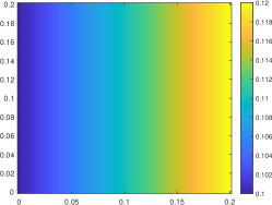
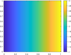
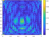
Experiment 1: Inversion within the Assumption of Theorem 3. In this experiment, we choose the quantities to satisfy the assumption (32) in Theorem 3. The computational domain is ; the attenuation coefficient is ; the anisotropy parameter is in the scattering kernel (33); the function is the solution of (13) with the boundary condition . Such choice gives the following numerical values:
On the other hand, we have for any anisotropy parameter between and , thus
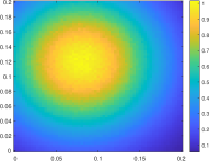
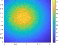
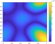
We test the Neumann series inversion with a smooth source
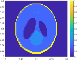
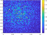
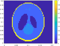
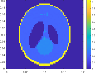
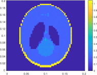
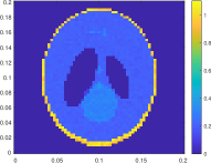
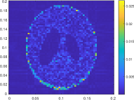
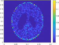
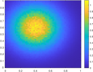
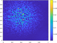
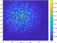
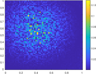
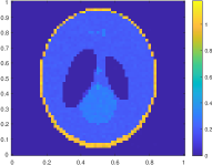
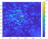
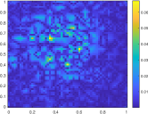
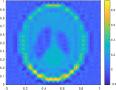
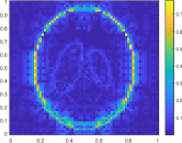
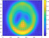
and a discontinuous source Shepp-Logan phantom, see Figure 3. The reconstructions with different levels of noises are illustrated in Figure 3 and Figure 3, respectively.


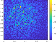


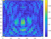
Experiment 2: Inversion beyond the Assumption of Theorem 3. The Neumann series in Theorem 3 was proved convergent under the sufficient condition (32). Here we also test the case when this condition fails. The experiment shows the series still converges in certain circumstances when the condition is violated.
We choose the computational domain , the attenuation coefficient . The constant , the anisotropy parameter , and the adjoint solution with remain the same as in Experiment 1. Notice that so the assumption (32) does not hold. In this case, the well-posedness of the forward RTE is ensured by (10) but not by (11). This is because
However, the first bound we obtained in (31) is never less than 1, as was explained before Theorem 3. This numerical experiment is therefore not covered by the proposed theorem.
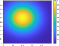
We test the Neumann series inversion with a smooth source
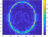
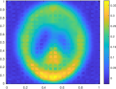
and the discontinuous Shepp-Logan phantom (see Figure 6). The reconstructions with different levels of noises are illustrated in Figure 6 and Figure 6, respectively.
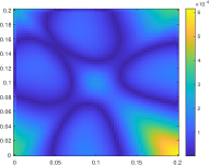
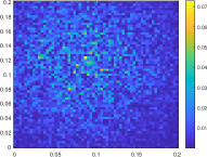
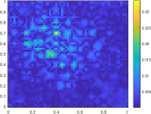
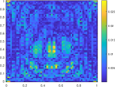
Experiment 3: Inversion with Theorem 5. We test the Fredholm inversion Theorem 5 in this experiment. Choose the computational domain , the attenuation coefficient (see Figure 3), in the scattering kernel (33), the adjoint RTE solution with .
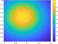
We test the Fredholm inversion with the smooth source (see Figure 6) and the discontinuous Shepp-Logan phantom (see Figure 3). The reconstructions with different levels of noises are illustrated in Figure 8 and Figure 8, respectively.
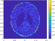
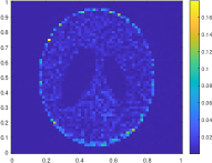
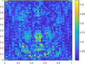
Experiment 4: Inversion with Theorem 5: Error Analysis. The errors in the reconstruction of the Shepp-Logan phantom is substantial. This is mostly due to our choice of the basis (36) in the discretization. The basis there consists only of smooth polynomials or pyramid-shaped functions , which fail to effectively represent a discontinuous function like the Shepp-Logan phantom. In order to justify this, we filter the phantom with a 2D Gaussian kernel with standard deviation 3 to get a smoother phantom (see Figure 10) and re-run the experiment. Then the errors in the reconstructions are greatly mitigated, as is illustrated in Figure 10. The experiment shows that suitable bases are critical for the success of the Fredholm inversion.


5. Conclusion
.
In this paper, we studied the ultrasound modulated biolumnescence tomography. Assuming knowledge of the attenuation coefficient , the scattering kernel and the domain , we proved that the isotropic source can be uniquely and stably reconstructed from the internal data in Theorem 3 and Theorem 5. The key step of the Fredholm method is to find a proper basis to reduce the approximation error in (36). The reconstructive procedures for are provided and numerically implemented in several experiments, in the presence or absence of noise, to demonstrate the efficiency of the reconstruction.
Appendix A Proof of Lemma 2
Proof of Lemma 2.
Let and Since and are uniformly positive, and the operator obtained by solving the transport equation are uniformly positive. Moreover the solution if is the solution to the ballistic equation with boundary condition , then is uniformly positive. Then it follows from the collision expansion form of the solution
(see for example equation 2.28 in [10]) that is uniformly positive and the result follows. ∎
References
- [1] Valeri Agoshkov. Boundary Value Problems for Transport Equations. Birkhauser Boston Inc., USA, 1998.
- [2] H. Ammari, E. Bossy, J. Garnier, L.H. Nguyen, and L. Seppecher. A reconstruction algorithm for ultrasound-modulated diffuse optical tomography. Proc. Amer. Math. Soc., 142:3221–3236, 2014.
- [3] H. Ammari, J. Garnier, L.H. Nguyen, and L. Seppecher. Reconstruction of a piecewise smooth absorption coefficient by an acousto-optic process. Comm. PDE., 38:1737–1762, 2013.
- [4] H. Ammari, L.H. Nguyen, and L. Seppecher. Reconstruction and stability in acousto-optic imaging for absorption maps with bounded variation. J. Functional Analysis, 267:4361–4398, 2014.
- [5] Davison B. and J.B. Sykes. Neutron Transport Theory. Oxford University Press, 1958.
- [6] G. Bal. Hybrid inverse problems and internal functionals. Inside Out II, MSRI Publications, 60:325–368, 2012.
- [7] G. Bal. Cauchy problem for ultrasound-modulated eit. Anal. PDE, 6(4):751–773, 2013.
- [8] G. Bal and S. Moskow. Local inversions in ultrasound modulated optical tomography. Inv. Prob., 30(2):025005, 2014.
- [9] G. Bal and A. Tamasan. Inverse source problems in transport equations. SIAM J. Math. Anal., 39(1):57–76, 2007.
- [10] Guillaume Bal, Francis J Chung, and John C Schotland. Ultrasound modulated bioluminescence tomography and controllability of the radiative transport equation. SIAM Journal on Mathematical Analysis, 48(2):1332–1347, 2016.
- [11] Guillaume Bal and John C Schotland. Inverse scattering and acousto-optic imaging. Physical review letters, 104(4):043902, 2010.
- [12] Guillaume Bal and John C Schotland. Ultrasound-modulated bioluminescence tomography. Physical Review E, 89(3):031201, 2014.
- [13] F.J. Chung, J. Hoskins, and J.C. Schotland. Coherent acousto-optic tomography with diffuse light. Optics Lett., 45(7):1623–1626, 2020.
- [14] F.J. Chung, J. Hoskins, and J.C. Schotland. A transport model for multi-frequency acousto-optic tomography. Inv. Prob., 36:064004, 2020.
- [15] F.J. Chung, R.-Y. Lai, and Q. Li. On diffusive scaling in acousto-optic imaging. Inv. Prob., to appear, 2020.
- [16] F.J. Chung and J.C. Schotland. Inverse transport and acousto-optic imaging. SIAM. J. Math. Anal., 49(6):4704–4721, 2017.
- [17] C. Contag and M.H. Bachmann. Advances in in vivo bioluminescence imaging of gene expression. Annu. Rev. Biomed. Eng., 4:235–260, 2002.
- [18] Robert Dautray and Jacques-Louis Lions. Mathematical Analysis and Numerical Methods for Science and Technology: Vol 6. Springer, 2000.
- [19] Ronald DeVore and Guergana Petrova. The averaging lemma. Journal of the American Mathematical Society, 14(2):279–296, 2001.
- [20] N.T. Huynh, B.R. Hayes-Gill, F. Zhang, and S.P. Morgan. Ultrasound modulated imaging of luminescence generated within a scattering medium. J. Biomedical Optics, 18:020505, 2013.
- [21] Wei Li, Yang Yang, and Yimin Zhong. A hybrid inverse problem in the fluorescence ultrasound modulated optical tomography in the diffusive regime. SIAM Journal on Applied Mathematics, 79(1):356–376, 2019.
- [22] Wei Li, Yang Yang, and Yimin Zhong. Inverse transport problem in fluorescence ultrasound modulated optical tomography with angularly averaged measurements. Inverse Problems, 36(2):025011, 2020.
- [23] V. Ntziachristos, J. Ripoll, L.H.V. Wang, and R. Weissleder. Looking and listening to light: the evolution of whole-body photonic imaging. Nat. Biotech., 23:313–320, 2005.
- [24] P. Stefanov and G. Uhlmann. An inverse problem in optical molecular imaging. Anal. PDE, 1:115–126, 2008.
- [25] Cheng Wang, Qiwei Sheng, and Weimin Han. A discrete-ordinate discontinuous-streamline diffusion method for the radiative transfer equation. Communications in Computational Physics, 20(5):1443–1465, 2016.