The Sivers Asymmetry in Hadronic Dijet Production

Zhong-Bo Kang zkang@physics.ucla.edu Department of Physics and Astronomy, University of California, Los Angeles, California 90095, USA Mani L. Bhaumik Institute for Theoretical Physics, University of California, Los Angeles, California 90095, USA Center for Frontiers in Nuclear Science, Stony Brook University, Stony Brook, New York 11794, USA    Kyle Lee kylelee@lbl.gov Nuclear Science Division, Lawrence Berkeley National Laboratory, Berkeley, California 94720, USA C.N. Yang Institute for Theoretical Physics, Stony Brook University, Stony Brook, New York 11794, USA Department of Physics and Astronomy, Stony Brook University, Stony Brook, New York 11794, USA    Ding Yu Shao dingyu.shao@cern.ch Department of Physics and Astronomy, University of California, Los Angeles, California 90095, USA Mani L. Bhaumik Institute for Theoretical Physics, University of California, Los Angeles, California 90095, USA Center for Frontiers in Nuclear Science, Stony Brook University, Stony Brook, New York 11794, USA    John Terry johndterry@physics.ucla.edu Department of Physics and Astronomy, University of California, Los Angeles, California 90095, USA Mani L. Bhaumik Institute for Theoretical Physics, University of California, Los Angeles, California 90095, USA
Abstract

We study the single spin asymmetry in the back-to-back dijet production in transversely polarized proton-proton collisions. Such an asymmetry is generated by the Sivers functions in the incoming polarized proton. We propose a QCD formalism in terms of the transverse momentum dependent parton distribution functions, which allow us to resum the large logarithms that arise in the perturbative calculations. We make predictions for the Sivers asymmetry of hadronic dijet production at the kinematic region that is relevant to the experiment at the Relativistic Heavy Ion Collider (RHIC). We further compute the spin asymmetries in the selected positive and negative jet charge bins, to separate the contributions from u𝑢u- and d𝑑d-quark Sivers functions. We find that both the sign and size of our numerical results are roughly consistent with the preliminary results from the STAR collaboration at the RHIC.

I Introduction

Exploring transverse momentum dependent parton distribution functions (TMD PDFs) has become one of the major research topics in hadron physics in recent years Boer:2011fh . TMD PDFs provide three-dimensional (3D) imaging of the nucleon in both the longitudinal and transverse momentum space, which is one of the scientific pillars at the future Electron-Ion Collider Accardi:2012qut . Such 3D imaging of the nucleon offers novel insights into the highly nontrivial non-perturbative QCD dynamics and correlations Aidala:2020mzt .

Sivers function is one of the most studied TMD PDFs in the community. It describes the distribution of unpolarized partons inside a transversely polarized nucleon, through a correlation between the transverse spin of the nucleon and the transverse momentum of the parton with respect to the nucleon’s moving direction. The Sivers function was first introduced by Sivers in 1990s Sivers:1989cc ; Sivers:1990fh to describe the large single transverse spin asymmetries observed in single inclusive particle production in hadronic collisions, see e.g. Antille:1980th ; Adams:1991rw . Since then, large single spin asymmetries have also been consistently observed in proton-proton collisions in high energy experiments at the Relativistic Heavy Ion Collider (RHIC) Adams:2003fx ; Arsene:2008aa ; Abelev:2008af ; Adamczyk:2012xd ; Adare:2013ekj ; Adamczyk:2017wld . On the theoretical side, understanding the precise origin of such large spin asymmetries has triggered extensive research in the QCD community Kane:1978nd ; Qiu:1991pp ; Kouvaris:2006zy ; Kang:2010zzb ; Kang:2011hk ; Metz:2012ct ; Gamberg:2013kla ; Kanazawa:2014dca ; Gamberg:2017gle . The difficulty in understanding such asymmetries for single hadron production (such as pions) in proton-proton collisions lies in the fact that they could receive contributions from many different correlations. Besides Sivers type correlations, whose collinear version is referred to as the Qiu-Sterman function Qiu:1991pp ; Qiu:1991wg in the incoming nucleon, there could also be similar correlations in the hadronization process when the parton fragments into the hadrons Kang:2010zzb ; Metz:2012ct ; Kanazawa:2010au ; Kanazawa:2014dca ; Gamberg:2017gle . See Cammarota:2020qcw for a recent development along this direction.

Simultaneously the Sivers asymmetry has also been studied in semi-inclusive deep inelastic scattering (SIDIS) by HERMES collaboration at DESY Airapetian:2009ae ; Airapetian:2020zzo , COMPASS collaboration at CERN Adolph:2012sp ; Adolph:2016dvl , and Jefferson Lab Qian:2011py . Because of the semi-inclusive nature of the process, one can isolate the contribution from the Sivers function via different azimuthal angular modulations Bacchetta:2006tn . One of the remarkable and unique properties of the Sivers functions is its non-universality nature. For example, based on parity and time-reversal invariance of QCD, one can show that quark Sivers functions in SIDIS are opposite to those in the Drell-Yan process Brodsky:2002rv ; Collins:2002kn ; Boer:2003cm . Such a sign change has been studied and confirmed experimentally Aghasyan:2017jop ; Adamczyk:2015gyk ; Kang:2009bp ; Anselmino:2016uie , though additional work remains to be done to quantify the change in more details Aschenauer:2016our .

Sivers effect has been continuously studied in proton-proton collisions at the RHIC. In order to eliminate the contributions from the spin correlations in the fragmentation process, the Sivers asymmetry for jet production processes has been explored in the experiment Bland:2013pkt ; Adamczyk:2017wld ; Abelev:2007ii . In particular, back-to-back dijet production in transversely polarized proton-proton collisions was proposed by Boer and Vogelsang in 2003 as a unique opportunity at the RHIC Boer:2003tx . Active investigation has been performed both experimentally Abelev:2007ii and theoretically Bomhof:2007su ; Vogelsang:2007jk ; Qiu:2007ar . On the experimental side, the Sivers asymmetry for dijet production was found to be quite small, largely due to the cancellation between u𝑢u- and d𝑑d-quark Sivers functions, which have similar size but opposite sign Echevarria:2014xaa ; Bacchetta:2020gko ; Cammarota:2020qcw . On the theoretical side, dijet production in proton-proton collisions is also subject to TMD factorization breaking Collins:2007nk ; Rogers:2010dm . These have slowed down the efforts in the detailed study of the Sivers effect in the dijet production.

Recently, there have been renewed experimental and theoretical interests for jet production processes. Experimentally, the STAR collaboration at the RHIC is analyzing the new data for dijet Sivers asymmetry, and is exploring a novel method based on a charge weighting method in separating the contributions from individual u𝑢u and d𝑑d-quark Sivers functions bnltalk . The PHENIX collaboration at the RHIC is exploring the TMD factorization breaking effects via back-to-back dihadron and photon-hadron production in proton-proton collisions Adare:2016bug ; Aidala:2018bjf . Theoretically, there have been efforts in performing QCD resummation in back-to-back dijet Sun:2014gfa ; Sun:2015doa and vector boson-jet production Buffing:2018ggv ; Chien:2019gyf ; Chien:2020hzh . At the same time, a theoretical framework has been developed to study spin asymmetries in specific jet charge bin Kang:2020fka , which would facilitate the analysis of the dijet spin asymmetries by the STAR collaboration. In light of all these activities, we set out to develop a resummation formalism for studying the Sivers asymmetry in back-to-back dijet production in transversely polarized proton-proton collisions. We make predictions for the dijet Sivers asymmetry in the kinematics relevant to the RHIC energy, to be compared with the experimental measurement in the near future.

The rest of the paper is organized as follows. In Section II, we summarized the QCD formalism for dijet production in both unpolarized and polarized scatterings, and we provide a few remarks about our formalism. In Section III, we provide a procedure and demonstrate how to compute the process-dependent polarized hard functions in the color matrix form. In Section IV, we present the renormalization group evolution of all the relevant functions in our formalism, and we provide the final resummation formula. Section V is devoted to the phenomenological studies, where we make predictions for dijet Sivers asymmetry in the kinematic region relevant to the experiment at the RHIC. Since we are mainly interested in the Sivers asymmetry in the forward rapidity region where quark contributions dominate, we consider only the quark Sivers contribution and neglect the gluon Sivers contribution. We summarize our paper in Section VI.

II QCD formalism for dijet production

In this paper, we study back-to-back dijet production in transversely polarized proton-proton collisions in the center-of mass frame,

p(PA,S)+p(PB)J1(yc,P1)+J2(yd,P2)+X,𝑝subscript𝑃𝐴subscript𝑆perpendicular-to𝑝subscript𝑃𝐵subscript𝐽1subscript𝑦𝑐subscript𝑃perpendicular-to1absentsubscript𝐽2subscript𝑦𝑑subscript𝑃perpendicular-to2absent𝑋\displaystyle p(P_{A},\vec{S}_{\perp})+p(P_{B})\to J_{1}(y_{c},\vec{P}_{1\perp})+J_{2}(y_{d},\vec{P}_{2\perp})+X\,, (1)

where the polarized proton with the momentum PAsubscript𝑃𝐴P_{A} and the transverse spin Ssubscript𝑆perpendicular-to\vec{S}_{\perp} is moving in the +z𝑧+z-direction, while the unpolarized proton with the momentum PBsubscript𝑃𝐵P_{B} is moving in the z𝑧-z-direction, and we have the center-of-mass energy s=(PA+PB)2𝑠superscriptsubscript𝑃𝐴subscript𝑃𝐵2s=(P_{A}+P_{B})^{2}. The produced two jets J1subscript𝐽1J_{1} and J2subscript𝐽2J_{2} have rapidities yc,dsubscript𝑦𝑐𝑑y_{c,d} and transverse momenta P1subscript𝑃perpendicular-to1absent\vec{P}_{1\perp} and P2subscript𝑃perpendicular-to2absent\vec{P}_{2\perp}, respectively.

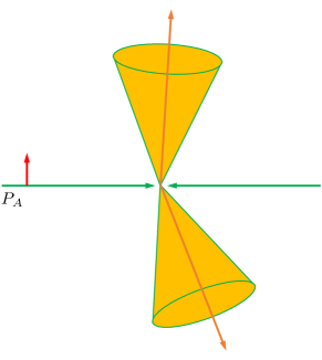
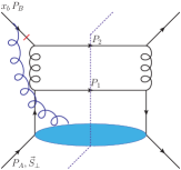
Refer to caption
Figure 1: Illustration of back-to-back dijet production in transversely polarized proton-proton collisions: p(PA,S)+p(PB)J1(yc,P1)+J2(yd,P2)+X𝑝subscript𝑃𝐴subscript𝑆perpendicular-to𝑝subscript𝑃𝐵subscript𝐽1subscript𝑦𝑐subscript𝑃perpendicular-to1absentsubscript𝐽2subscript𝑦𝑑subscript𝑃perpendicular-to2absent𝑋p(P_{A},\vec{S}_{\perp})+p(P_{B})\to J_{1}(y_{c},\vec{P}_{1\perp})+J_{2}(y_{d},\vec{P}_{2\perp})+X. The polarized proton with momentum PAsubscript𝑃𝐴P_{A} and transverse spin Ssubscript𝑆perpendicular-to\vec{S}_{\perp} is moving in +z𝑧+z-direction, while the unpolarized proton with momentum PBsubscript𝑃𝐵P_{B} is moving in z𝑧-z-direction. We have jet rapidities yc,dsubscript𝑦𝑐𝑑y_{c,d} and transverse momenta P1subscript𝑃perpendicular-to1absent\vec{P}_{1\perp} and P2subscript𝑃perpendicular-to2absent\vec{P}_{2\perp}, respectively. The dijet transverse momentum imbalance is defined as q=P1+P2subscript𝑞perpendicular-tosubscript𝑃perpendicular-to1absentsubscript𝑃perpendicular-to2absent\vec{q}_{\perp}=\vec{P}_{1\perp}+\vec{P}_{2\perp}. Sivers asymmetry is generated due to the correlation between Ssubscript𝑆perpendicular-to\vec{S}_{\perp} and qsubscript𝑞perpendicular-to\vec{q}_{\perp}.

These jets will be reconstructed via a suitable jet algorithm Cacciari:2011ma and in the rest of the paper, we consider both of them to be anti-kTsubscript𝑘𝑇k_{T} jets with jet radii R𝑅R. In order to access the transverse motion of the partons inside the protons, we concentrate in the back-to-back region where the transverse momentum imbalance qsubscript𝑞perpendicular-toq_{\perp} is small. Here we define the average transverse momentum Psubscript𝑃perpendicular-toP_{\perp} of the two jets and the transverse momentum imbalance qsubscript𝑞perpendicular-to\vec{q}_{\perp} as follows

P=|P1P2|/2,q=P1+P2,formulae-sequencesubscript𝑃perpendicular-tosubscript𝑃perpendicular-to1absentsubscript𝑃perpendicular-to2absent2subscript𝑞perpendicular-tosubscript𝑃perpendicular-to1absentsubscript𝑃perpendicular-to2absent\displaystyle P_{\perp}=|\vec{P}_{1\perp}-\vec{P}_{2\perp}|/2\,,\qquad\vec{q}_{\perp}=\vec{P}_{1\perp}+\vec{P}_{2\perp}\,, (2)

where one has qPmuch-less-thansubscript𝑞perpendicular-tosubscript𝑃perpendicular-toq_{\perp}\ll P_{\perp} in the back-to-back region. The production of such back-to-back dijets is illustrated in Fig. 1. In the transversely polarized proton-proton collisions, the transverse spin vector Ssubscript𝑆perpendicular-to\vec{S}_{\perp} of the incoming proton and the transverse momentum imbalance qsubscript𝑞perpendicular-to\vec{q}_{\perp} of the two jets will be correlated, as advocated in Boer:2003tx . This correlation is accounted for in the Sivers function, which leads to a sin(ϕqϕS)sinsubscriptitalic-ϕ𝑞subscriptitalic-ϕ𝑆\hbox{sin}(\phi_{q}-\phi_{S})-azimuthal modulation in the cross section between ϕqsubscriptitalic-ϕ𝑞\phi_{q} and ϕSsubscriptitalic-ϕ𝑆\phi_{S}, the azimuthal angles of qsubscript𝑞perpendicular-to\vec{q}_{\perp} and Ssubscript𝑆perpendicular-to\vec{S}_{\perp}, respectively. Below we summarize the factorized formalisms for dijet production in both unpolarized and polarized proton-proton collisions, and we provide more details for the relevant ingredients in the next section.

II.1 Dijet unpolarized cross section

In the back-to-back region where qPmuch-less-thansubscript𝑞perpendicular-tosubscript𝑃perpendicular-toq_{\perp}\ll P_{\perp}, within the framework of soft-collinear effective theory (SCET) Bauer:2000ew ; Bauer:2000yr ; Bauer:2001ct ; Bauer:2001yt ; Bauer:2002nz , one can write down a factorized form for the unpolarized differential cross section

dσdycdyddP2d2q=𝑑𝜎𝑑subscript𝑦𝑐𝑑subscript𝑦𝑑𝑑superscriptsubscript𝑃perpendicular-to2superscript𝑑2subscript𝑞perpendicular-toabsent\displaystyle\frac{d\sigma}{dy_{c}dy_{d}dP_{\perp}^{2}d^{2}\vec{q}_{\perp}}= abcd116π2s^21Ninit11+δcdxafaunsub(xa,ka,μ,ν)xbfbunsub(xb,ka,μ,ν)subscript𝑎𝑏𝑐𝑑116superscript𝜋2superscript^𝑠21subscript𝑁init11subscript𝛿𝑐𝑑subscriptperpendicular-tosubscript𝑥𝑎subscriptsuperscript𝑓unsub𝑎subscript𝑥𝑎subscript𝑘perpendicular-to𝑎absent𝜇𝜈subscript𝑥𝑏subscriptsuperscript𝑓unsub𝑏subscript𝑥𝑏subscript𝑘perpendicular-to𝑎absent𝜇𝜈\displaystyle\sum_{abcd}\frac{1}{16\pi^{2}\hat{s}^{2}}\frac{1}{N_{\rm init}}\frac{1}{1+\delta_{cd}}\int_{\perp}\,x_{a}f^{\rm unsub}_{a}(x_{a},k_{a\perp},\mu,\nu)\,x_{b}f^{\rm unsub}_{b}(x_{b},k_{a\perp},\mu,\nu)
×Tr[𝑺abcd(λ,μ,ν)𝑯abcd(P,μ)]Jc(PR,μ)Sccs(kc,R,μ)Jd(PR,μ)Sdcs(kd,R,μ),absentTrdelimited-[]subscript𝑺𝑎𝑏𝑐𝑑subscript𝜆perpendicular-to𝜇𝜈subscript𝑯𝑎𝑏𝑐𝑑subscript𝑃perpendicular-to𝜇subscript𝐽𝑐subscript𝑃perpendicular-to𝑅𝜇subscriptsuperscript𝑆cs𝑐subscript𝑘perpendicular-to𝑐absent𝑅𝜇subscript𝐽𝑑subscript𝑃perpendicular-to𝑅𝜇subscriptsuperscript𝑆cs𝑑subscript𝑘perpendicular-to𝑑absent𝑅𝜇\displaystyle\times{\rm Tr}\left[\bm{S}_{ab\rightarrow cd}(\lambda_{\perp},\mu,\nu)\cdot\bm{H}_{ab\rightarrow cd}(P_{\perp},\mu)\right]J_{c}(P_{\perp}R,\mu)S^{\rm cs}_{c}(k_{c\perp},R,\mu)J_{d}(P_{\perp}R,\mu)S^{\rm cs}_{d}(k_{d\perp},R,\mu)\,, (3)

where s^=xaxbs^𝑠subscript𝑥𝑎subscript𝑥𝑏𝑠\hat{s}=x_{a}x_{b}s is the partonic center-of-mass energy, Ninitsubscript𝑁initN_{\rm init} is the corresponding spin- and color-averaged factor for each channel, while 1/(1+δcd)11subscript𝛿𝑐𝑑1/(1+\delta_{cd}) arises from the symmetry factor due to identical partons in the final state. We have used the following short-hand notation

=d2kad2kbd2kcd2kdd2λδ(2)(ka+kb+kc+kd+λq).subscriptperpendicular-tosuperscript𝑑2subscript𝑘perpendicular-to𝑎absentsuperscript𝑑2subscript𝑘perpendicular-to𝑏absentsuperscript𝑑2subscript𝑘perpendicular-to𝑐absentsuperscript𝑑2subscript𝑘perpendicular-to𝑑absentsuperscript𝑑2subscript𝜆perpendicular-tosuperscript𝛿2subscript𝑘perpendicular-to𝑎absentsubscript𝑘perpendicular-to𝑏absentsubscript𝑘perpendicular-to𝑐absentsubscript𝑘perpendicular-to𝑑absentsubscript𝜆perpendicular-tosubscript𝑞perpendicular-to\displaystyle\int_{\perp}=\int d^{2}\vec{k}_{a\perp}d^{2}\vec{k}_{b\perp}d^{2}\vec{k}_{c\perp}d^{2}\vec{k}_{d\perp}d^{2}\vec{\lambda}_{\perp}\delta^{(2)}(\vec{k}_{a\perp}+\vec{k}_{b\perp}+\vec{k}_{c\perp}+\vec{k}_{d\perp}+\vec{\lambda}_{\perp}-\vec{q}_{\perp})\,. (4)

In Eq. (II.1), faunsub(xa,ka,μ,ν)subscriptsuperscript𝑓unsub𝑎subscript𝑥𝑎subscript𝑘perpendicular-to𝑎absent𝜇𝜈f^{\rm unsub}_{a}(x_{a},k_{a\perp},\mu,\nu) and fbunsub(xb,kb,μ,ν)subscriptsuperscript𝑓unsub𝑏subscript𝑥𝑏subscript𝑘perpendicular-to𝑏absent𝜇𝜈f^{\rm unsub}_{b}(x_{b},k_{b\perp},\mu,\nu) are the so-called unsubtracted TMD PDFs, which carry the longitudinal momentum fractions xa,bsubscript𝑥𝑎𝑏x_{a,b} and the transverse momenta kasubscript𝑘perpendicular-to𝑎absentk_{a\perp} and kbsubscript𝑘perpendicular-to𝑏absentk_{b\perp} with respect to their corresponding proton. In our process, we have

xa=Ps(eyc+eyd),xb=Ps(eyc+eyd),formulae-sequencesubscript𝑥𝑎subscript𝑃perpendicular-to𝑠superscript𝑒subscript𝑦𝑐superscript𝑒subscript𝑦𝑑subscript𝑥𝑏subscript𝑃perpendicular-to𝑠superscript𝑒subscript𝑦𝑐superscript𝑒subscript𝑦𝑑\displaystyle x_{a}=\frac{P_{\perp}}{\sqrt{s}}\left(e^{y_{c}}+e^{y_{d}}\right)\,,\qquad x_{b}=\frac{P_{\perp}}{\sqrt{s}}\left(e^{-y_{c}}+e^{-y_{d}}\right)\,, (5)

where ycsubscript𝑦𝑐y_{c}, ydsubscript𝑦𝑑y_{d} are the rapidities of the two leading jets.

After performing Fourier transform for Eq. (II.1), we obtain the factorized formula in the coordinate b𝑏b-space as follows

dσdycdyddP2d2q=𝑑𝜎𝑑subscript𝑦𝑐𝑑subscript𝑦𝑑𝑑superscriptsubscript𝑃perpendicular-to2superscript𝑑2subscript𝑞perpendicular-toabsent\displaystyle\frac{d\sigma}{dy_{c}dy_{d}dP_{\perp}^{2}d^{2}\vec{q}_{\perp}}= abcd116π2s^21Ninit11+δcdd2b(2π)2eiqbxafaunsub(xa,b,μ,ν)xbfbunsub(xb,b,μ,ν)subscript𝑎𝑏𝑐𝑑116superscript𝜋2superscript^𝑠21subscript𝑁init11subscript𝛿𝑐𝑑superscript𝑑2𝑏superscript2𝜋2superscript𝑒𝑖subscript𝑞perpendicular-to𝑏subscript𝑥𝑎subscriptsuperscript𝑓unsub𝑎subscript𝑥𝑎𝑏𝜇𝜈subscript𝑥𝑏subscriptsuperscript𝑓unsub𝑏subscript𝑥𝑏𝑏𝜇𝜈\displaystyle\sum_{abcd}\frac{1}{16\pi^{2}\hat{s}^{2}}\frac{1}{N_{\rm init}}\frac{1}{1+\delta_{cd}}\int\frac{d^{2}\vec{b}}{(2\pi)^{2}}\,e^{i\vec{q}_{\perp}\cdot\vec{b}}\,x_{a}f^{\rm unsub}_{a}(x_{a},b,\mu,\nu)\,x_{b}f^{\rm unsub}_{b}(x_{b},b,\mu,\nu)
×Tr[𝑺abcd(b,μ,ν)𝑯abcd(P,μ)]Jc(PR,μ)Sccs(b,R,μ)Jd(PR,μ)Sdcs(b,R,μ),absentTrdelimited-[]subscript𝑺𝑎𝑏𝑐𝑑𝑏𝜇𝜈subscript𝑯𝑎𝑏𝑐𝑑subscript𝑃perpendicular-to𝜇subscript𝐽𝑐subscript𝑃perpendicular-to𝑅𝜇subscriptsuperscript𝑆cs𝑐𝑏𝑅𝜇subscript𝐽𝑑subscript𝑃perpendicular-to𝑅𝜇subscriptsuperscript𝑆cs𝑑𝑏𝑅𝜇\displaystyle\times{\rm Tr}\left[\bm{S}_{ab\rightarrow cd}(b,\mu,\nu)\cdot\bm{H}_{ab\rightarrow cd}(P_{\perp},\mu)\right]J_{c}(P_{\perp}R,\mu)S^{\rm cs}_{c}(b,R,\mu)J_{d}(P_{\perp}R,\mu)S^{\rm cs}_{d}(b,R,\mu)\,, (6)

where faunsub(xa,b,μ,ν)subscriptsuperscript𝑓unsub𝑎subscript𝑥𝑎𝑏𝜇𝜈f^{\rm unsub}_{a}(x_{a},b,\mu,\nu) and fbunsub(xb,b,μ,ν)subscriptsuperscript𝑓unsub𝑏subscript𝑥𝑏𝑏𝜇𝜈f^{\rm unsub}_{b}(x_{b},b,\mu,\nu) are the Fourier transform of faunsub(xa,ka,μ,ν)subscriptsuperscript𝑓unsub𝑎subscript𝑥𝑎subscript𝑘perpendicular-to𝑎absent𝜇𝜈f^{\rm unsub}_{a}(x_{a},k_{a\perp},\mu,\nu) and fbunsub(xb,kb,μ,ν)subscriptsuperscript𝑓unsub𝑏subscript𝑥𝑏subscript𝑘perpendicular-to𝑏absent𝜇𝜈f^{\rm unsub}_{b}(x_{b},k_{b\perp},\mu,\nu), respectively. On the other hand, 𝑯abcd(P,μ)subscript𝑯𝑎𝑏𝑐𝑑subscript𝑃perpendicular-to𝜇\bm{H}_{ab\rightarrow cd}(P_{\perp},\mu) is the hard function, while 𝑺abcd(b,μ,ν)subscript𝑺𝑎𝑏𝑐𝑑𝑏𝜇𝜈\bm{S}_{ab\to cd}(b,\mu,\nu) is a global soft function. Note that both the hard function 𝑯abcdsubscript𝑯𝑎𝑏𝑐𝑑\bm{H}_{ab\rightarrow cd} and the global soft function 𝑺abcdsubscript𝑺𝑎𝑏𝑐𝑑\bm{S}_{ab\to cd} are expressed in the matrix form in the color space and the trace Tr[]Trdelimited-[]{\rm Tr}[\cdots] is over the color. Such factorization of the hard and soft function into matrix form is essential to capture evolution effects between the hard scale Psimilar-toabsentsubscript𝑃perpendicular-to\sim P_{\perp} and the imbalance scale qsimilar-toabsentsubscript𝑞perpendicular-to\sim q_{\perp} Kidonakis:1998nf . Here μ𝜇\mu and ν𝜈\nu denotes renormalization and rapidity scales, separately. The rapidity scale ν𝜈\nu arises because both the TMD PDFs and the global soft functions have rapidity divergence Chiu:2011qc ; Chiu:2012ir , which are canceled between them as demonstrated below. This cancellation allows us to define rapidity divergence independent 𝑺~abcd(b,μ)subscript~𝑺𝑎𝑏𝑐𝑑𝑏𝜇\tilde{\bm{S}}_{ab\to cd}(b,\mu) by

𝑺abcd(b,μ,ν)=𝑺~abcd(b,μ)Sab(b,μ,ν),subscript𝑺𝑎𝑏𝑐𝑑𝑏𝜇𝜈subscript~𝑺𝑎𝑏𝑐𝑑𝑏𝜇subscript𝑆𝑎𝑏𝑏𝜇𝜈\displaystyle\bm{S}_{ab\to cd}(b,\mu,\nu)=\tilde{\bm{S}}_{ab\to cd}(b,\mu)S_{ab}(b,\mu,\nu)\,, (7)

where Sab(b,μ,ν)subscript𝑆𝑎𝑏𝑏𝜇𝜈S_{ab}(b,\mu,\nu) is the standard soft function appearing in usual Drell-Yan and SIDIS processes. This explicit redefinition allows us to subtract the rapidity divergence from the unsubtracted TMD PDFs to define the standard TMD PDFs fi(xi,b,μ)subscript𝑓𝑖subscript𝑥𝑖𝑏𝜇f_{i}(x_{i},b,\mu) that are free of rapidity divergence as Collins:2011zzd

faunsub(xa,b,μ,ν)fbunsub(xb,b,μ,ν)Sab(b,μ,ν)=fa(xa,b,μ)fb(xb,b,μ).subscriptsuperscript𝑓unsub𝑎subscript𝑥𝑎𝑏𝜇𝜈subscriptsuperscript𝑓unsub𝑏subscript𝑥𝑏𝑏𝜇𝜈subscript𝑆𝑎𝑏𝑏𝜇𝜈subscript𝑓𝑎subscript𝑥𝑎𝑏𝜇subscript𝑓𝑏subscript𝑥𝑏𝑏𝜇\displaystyle f^{\rm unsub}_{a}(x_{a},b,\mu,\nu)\,f^{\rm unsub}_{b}(x_{b},b,\mu,\nu)\,S_{ab}(b,\mu,\nu)=f_{a}(x_{a},b,\mu)\,f_{b}(x_{b},b,\mu)\,. (8)

Note that the properly-defined TMD PDFs fa(xa,b,μ)subscript𝑓𝑎subscript𝑥𝑎𝑏𝜇f_{a}(x_{a},b,\mu) and fb(xb,b,μ)subscript𝑓𝑏subscript𝑥𝑏𝑏𝜇f_{b}(x_{b},b,\mu) are no longer subject to the rapidity divergence and this is why there are no explicit ν𝜈\nu-dependence in the arguments any more. Such properly-defined unpolarized TMD PDFs are the same as those probed in the standard SIDIS and Drell-Yan processes.

The jet functions Jc(PR,μ)subscript𝐽𝑐subscript𝑃perpendicular-to𝑅𝜇J_{c}(P_{\perp}R,\mu) and Jd(PR,μ)subscript𝐽𝑑subscript𝑃perpendicular-to𝑅𝜇J_{d}(P_{\perp}R,\mu) in Eq. (II.1) describe the creation of anti-kTsubscript𝑘𝑇k_{T} jets from the partons c𝑐c and d𝑑d, respectively. Finally, Sccs(kc,R,μ)subscriptsuperscript𝑆cs𝑐subscript𝑘perpendicular-to𝑐absent𝑅𝜇S^{\rm cs}_{c}(k_{c\perp},R,\mu) and Sdcs(kd,R,μ)subscriptsuperscript𝑆cs𝑑subscript𝑘perpendicular-to𝑑absent𝑅𝜇S^{\rm cs}_{d}(k_{d\perp},R,\mu) are the collinear-soft functions. They describe soft gluon radiation with separations of order R𝑅R along the jet direction, which can resolve the substructure of the jet. If one performs the integration over the azimuthal angle of the vector b𝑏\vec{b}, we obtain the following expression

dσdycdyddP2d2q=𝑑𝜎𝑑subscript𝑦𝑐𝑑subscript𝑦𝑑𝑑superscriptsubscript𝑃perpendicular-to2superscript𝑑2subscript𝑞perpendicular-toabsent\displaystyle\frac{d\sigma}{dy_{c}dy_{d}dP_{\perp}^{2}d^{2}\vec{q}_{\perp}}= abcd116π2s^21Ninit11+δcd12π0𝑑bbJ0(qb)xafa(xa,b,μ)xbfb(xb,b,μ)subscript𝑎𝑏𝑐𝑑116superscript𝜋2superscript^𝑠21subscript𝑁init11subscript𝛿𝑐𝑑12𝜋superscriptsubscript0differential-d𝑏𝑏subscript𝐽0subscript𝑞perpendicular-to𝑏subscript𝑥𝑎subscript𝑓𝑎subscript𝑥𝑎𝑏𝜇subscript𝑥𝑏subscript𝑓𝑏subscript𝑥𝑏𝑏𝜇\displaystyle\sum_{abcd}\frac{1}{16\pi^{2}\hat{s}^{2}}\frac{1}{N_{\rm init}}\frac{1}{1+\delta_{cd}}\frac{1}{2\pi}\int_{0}^{\infty}db\,b\,J_{0}(q_{\perp}b)\,x_{a}f_{a}(x_{a},b,\mu)\,x_{b}f_{b}(x_{b},b,\mu)
×Tr[𝑺~abcd(b,μ)𝑯abcd(P,μ)]Jc(PR,μ)Sccs(b,R,μ)Jd(PR,μ)Sdcs(b,R,μ),absentTrdelimited-[]subscript~𝑺𝑎𝑏𝑐𝑑𝑏𝜇subscript𝑯𝑎𝑏𝑐𝑑subscript𝑃perpendicular-to𝜇subscript𝐽𝑐subscript𝑃perpendicular-to𝑅𝜇subscriptsuperscript𝑆cs𝑐𝑏𝑅𝜇subscript𝐽𝑑subscript𝑃perpendicular-to𝑅𝜇subscriptsuperscript𝑆cs𝑑𝑏𝑅𝜇\displaystyle\times{\rm Tr}\left[\tilde{\bm{S}}_{ab\rightarrow cd}(b,\mu)\cdot\bm{H}_{ab\rightarrow cd}(P_{\perp},\mu)\right]J_{c}(P_{\perp}R,\mu)S^{\rm cs}_{c}(b,R,\mu)J_{d}(P_{\perp}R,\mu)S^{\rm cs}_{d}(b,R,\mu)\,, (9)

where J0subscript𝐽0J_{0} is the Bessel function of order zero.

II.2 Dijet Sivers asymmetry

In the transversely polarized proton-proton collisions, the Sivers function will lead to a spin asymmetry in the cross section when one flips the transverse spin of the incoming proton. We thus define the difference in the cross section as dΔσ(S)=[dσ(S)dσ(S)]/2𝑑Δ𝜎subscript𝑆perpendicular-todelimited-[]𝑑𝜎subscript𝑆perpendicular-to𝑑𝜎subscript𝑆perpendicular-to2d\Delta\sigma(S_{\perp})=\left[d\sigma(S_{\perp})-d\sigma(-S_{\perp})\right]/2. One can write down a similar factorized formula for such a spin-dependent differential cross section following Eq. (II.1), and it is given by

dΔσ(S)dycdyddP2d2q=𝑑Δ𝜎subscript𝑆perpendicular-to𝑑subscript𝑦𝑐𝑑subscript𝑦𝑑𝑑superscriptsubscript𝑃perpendicular-to2superscript𝑑2subscript𝑞perpendicular-toabsent\displaystyle\frac{d\Delta\sigma(S_{\perp})}{dy_{c}dy_{d}dP_{\perp}^{2}d^{2}\vec{q}_{\perp}}= abcd116π2s^21Ninit11+δcd1MϵαβSαkaβxaf1Ta,unsub(xa,ka,μ,ν)xbfbunsub(xb,ka,μ,ν)subscript𝑎𝑏𝑐𝑑116superscript𝜋2superscript^𝑠21subscript𝑁init11subscript𝛿𝑐𝑑subscriptperpendicular-to1𝑀subscriptitalic-ϵ𝛼𝛽superscriptsubscript𝑆perpendicular-to𝛼superscriptsubscript𝑘perpendicular-to𝑎absent𝛽subscript𝑥𝑎superscriptsubscript𝑓1𝑇perpendicular-toabsent𝑎unsubsubscript𝑥𝑎subscript𝑘perpendicular-to𝑎absent𝜇𝜈subscript𝑥𝑏subscriptsuperscript𝑓unsub𝑏subscript𝑥𝑏subscript𝑘perpendicular-to𝑎absent𝜇𝜈\displaystyle\sum_{abcd}\frac{1}{16\pi^{2}\hat{s}^{2}}\frac{1}{N_{\rm init}}\frac{1}{1+\delta_{cd}}\int_{\perp}\,\frac{1}{M}\epsilon_{\alpha\beta}\,S_{\perp}^{\alpha}\,k_{a\perp}^{\beta}\,x_{a}f_{1T}^{\perp a,\,{\rm unsub}}(x_{a},k_{a\perp},\mu,\nu)\,x_{b}f^{\rm unsub}_{b}(x_{b},k_{a\perp},\mu,\nu)
×Tr[𝑺abcd(λ,μ,ν)𝑯abcdSivers(P,μ)]Jc(PR,μ)Sccs(kc,R,μ)Jd(PR,μ)Sdcs(kd,R,μ),absentTrdelimited-[]subscript𝑺𝑎𝑏𝑐𝑑subscript𝜆perpendicular-to𝜇𝜈superscriptsubscript𝑯𝑎𝑏𝑐𝑑Siverssubscript𝑃perpendicular-to𝜇subscript𝐽𝑐subscript𝑃perpendicular-to𝑅𝜇subscriptsuperscript𝑆cs𝑐subscript𝑘perpendicular-to𝑐absent𝑅𝜇subscript𝐽𝑑subscript𝑃perpendicular-to𝑅𝜇subscriptsuperscript𝑆cs𝑑subscript𝑘perpendicular-to𝑑absent𝑅𝜇\displaystyle\times{\rm Tr}\left[\bm{S}_{ab\rightarrow cd}(\lambda_{\perp},\mu,\nu)\cdot\bm{H}_{ab\rightarrow cd}^{\rm Sivers}(P_{\perp},\mu)\right]J_{c}(P_{\perp}R,\mu)S^{\rm cs}_{c}(k_{c\perp},R,\mu)J_{d}(P_{\perp}R,\mu)S^{\rm cs}_{d}(k_{d\perp},R,\mu)\,, (10)

where ϵαβsubscriptitalic-ϵ𝛼𝛽\epsilon_{\alpha\beta} is a two-dimensional asymmetric tensor with ϵ12=+1subscriptitalic-ϵ121\epsilon_{12}=+1, and we have replaced the unpolarized TMD PDF in Eq. (II.1) by the Sivers function in the above equation following the so-called Trento convention Bacchetta:2004jz ,

faunsub(xa,ka,μ,ν)1MϵαβSαkaβf1Ta,unsub(xa,ka,μ,ν).superscriptsubscript𝑓𝑎unsubsubscript𝑥𝑎subscript𝑘perpendicular-to𝑎absent𝜇𝜈1𝑀subscriptitalic-ϵ𝛼𝛽superscriptsubscript𝑆perpendicular-to𝛼superscriptsubscript𝑘perpendicular-to𝑎absent𝛽superscriptsubscript𝑓1𝑇perpendicular-toabsent𝑎unsubsubscript𝑥𝑎subscript𝑘perpendicular-to𝑎absent𝜇𝜈\displaystyle f_{a}^{\rm unsub}(x_{a},k_{a\perp},\mu,\nu)\rightarrow\frac{1}{M}\epsilon_{\alpha\beta}\,S_{\perp}^{\alpha}\,k_{a\perp}^{\beta}\,f_{1T}^{\perp a,\,{\rm unsub}}(x_{a},k_{a\perp},\mu,\nu)\,. (11)

Note that we have also assumed that the global soft function 𝑺abcd(λ,μ,ν)subscript𝑺𝑎𝑏𝑐𝑑subscript𝜆perpendicular-to𝜇𝜈\bm{S}_{ab\rightarrow cd}(\lambda_{\perp},\mu,\nu) stays the same as that of the unpolarized collisions in Eq. (II.1). Although this is a reasonable assumption since the soft gluon radiation should be spin-independent Kelley:2010fn ; Echevarria:2015usa , this has to be carefully checked. In fact, Ref. Liu:2020jjv shows in explicit calculations at one-loop level that soft functions in the polarized case can be different from the unpolarized counterpart beyond leading logarithmic accuracy, which is an indication of TMD factorization breaking. In this respect, our starting point Eq. (II.2) will be the best assumption at hand that takes a factorized form. We show the RG consistency for this factorized form, and we also demonstrate how we derive the process-dependent hard functions 𝑯abcdSivers(P,μ)superscriptsubscript𝑯𝑎𝑏𝑐𝑑Siverssubscript𝑃perpendicular-to𝜇\bm{H}_{ab\rightarrow cd}^{\rm Sivers}(P_{\perp},\mu) for the polarized scattering. We leave a detailed study on the numerical impact of any TMD factorization breaking effects for future investigation.

Performing Fourier transform from the transverse momentum space into the b𝑏b-space, we obtain

dΔσ(S)dycdyddP2d2q=𝑑Δ𝜎subscript𝑆perpendicular-to𝑑subscript𝑦𝑐𝑑subscript𝑦𝑑𝑑superscriptsubscript𝑃perpendicular-to2superscript𝑑2subscript𝑞perpendicular-toabsent\displaystyle\frac{d\Delta\sigma(S_{\perp})}{dy_{c}dy_{d}dP_{\perp}^{2}d^{2}\vec{q}_{\perp}}= abcd116π2s^21Ninit11+δcdϵαβSαd2b(2π)2eiqbxaf1Ta(β)(xa,b,μ)xbfb(xb,b,μ)subscript𝑎𝑏𝑐𝑑116superscript𝜋2superscript^𝑠21subscript𝑁init11subscript𝛿𝑐𝑑subscriptitalic-ϵ𝛼𝛽superscriptsubscript𝑆perpendicular-to𝛼superscript𝑑2𝑏superscript2𝜋2superscript𝑒𝑖subscript𝑞perpendicular-to𝑏subscript𝑥𝑎superscriptsubscript𝑓1𝑇perpendicular-toabsent𝑎𝛽subscript𝑥𝑎𝑏𝜇subscript𝑥𝑏subscript𝑓𝑏subscript𝑥𝑏𝑏𝜇\displaystyle\sum_{abcd}\frac{1}{16\pi^{2}\hat{s}^{2}}\frac{1}{N_{\rm init}}\frac{1}{1+\delta_{cd}}\epsilon_{\alpha\beta}\,S_{\perp}^{\alpha}\int\frac{d^{2}\vec{b}}{(2\pi)^{2}}\,e^{i\vec{q}_{\perp}\cdot\vec{b}}\,x_{a}f_{1T}^{\perp\,a(\beta)}(x_{a},b,\mu)\,x_{b}f_{b}(x_{b},b,\mu)
×Tr[𝑺~abcd(b,μ)𝑯abcdSivers(P,μ)]Jc(PR,μ)Sccs(b,R,μ)Jd(PR,μ)Sdcs(b,R,μ),absentTrdelimited-[]subscript~𝑺𝑎𝑏𝑐𝑑𝑏𝜇superscriptsubscript𝑯𝑎𝑏𝑐𝑑Siverssubscript𝑃perpendicular-to𝜇subscript𝐽𝑐subscript𝑃perpendicular-to𝑅𝜇subscriptsuperscript𝑆cs𝑐𝑏𝑅𝜇subscript𝐽𝑑subscript𝑃perpendicular-to𝑅𝜇subscriptsuperscript𝑆cs𝑑𝑏𝑅𝜇\displaystyle\times{\rm Tr}\left[\tilde{\bm{S}}_{ab\rightarrow cd}(b,\mu)\cdot\bm{H}_{ab\rightarrow cd}^{\rm Sivers}(P_{\perp},\mu)\right]J_{c}(P_{\perp}R,\mu)S^{\rm cs}_{c}(b,R,\mu)J_{d}(P_{\perp}R,\mu)S^{\rm cs}_{d}(b,R,\mu)\,, (12)

where we have already used Eq. (7) to rewrite the unsubtracted unpolarized TMD PDF and Sivers function in terms of the properly defined versions which are free of rapidity divergence. Here f1Ta(β)(xa,b,μ)superscriptsubscript𝑓1𝑇perpendicular-toabsent𝑎𝛽subscript𝑥𝑎𝑏𝜇f_{1T}^{\perp\,a(\beta)}(x_{a},b,\mu) is the Fourier transform of the Sivers function,

f1Ta(β)(xa,b,μ)=superscriptsubscript𝑓1𝑇perpendicular-toabsent𝑎𝛽subscript𝑥𝑎𝑏𝜇absent\displaystyle f_{1T}^{\perp\,a(\beta)}(x_{a},b,\mu)=\, 1Md2kaeikabkaβf1Ta(xa,ka,μ),1𝑀superscript𝑑2subscript𝑘perpendicular-to𝑎absentsuperscript𝑒𝑖subscript𝑘perpendicular-to𝑎absent𝑏superscriptsubscript𝑘perpendicular-to𝑎absent𝛽superscriptsubscript𝑓1𝑇perpendicular-toabsent𝑎subscript𝑥𝑎subscript𝑘perpendicular-to𝑎absent𝜇\displaystyle\frac{1}{M}\int d^{2}\vec{k}_{a\perp}\,e^{-i\vec{k}_{a\perp}\cdot\vec{b}}\,k_{a\perp}^{\beta}f_{1T}^{\perp\,a}(x_{a},k_{a\perp},\mu)\,,
\displaystyle\equiv\, (ibβ2)f^1Ta(xa,b,μ),𝑖superscript𝑏𝛽2superscriptsubscript^𝑓1𝑇perpendicular-toabsent𝑎subscript𝑥𝑎𝑏𝜇\displaystyle\left(\frac{ib^{\beta}}{2}\right)\hat{f}_{1T}^{\perp\,a}(x_{a},b,\mu)\,, (13)

where we have used the fact that the integration in the first line would be proportional to bβsuperscript𝑏𝛽b^{\beta}, and we thus factored bβsuperscript𝑏𝛽b^{\beta} out explicitly in the second line 111To make the matching coefficient normalized to 1 at the lowest order in Eq. (15), we include the additional factor of i/2𝑖2i/2 in Eq. (13).. The remaining part of the Sivers function is now denoted as f^1Ta(xa,b,μ)superscriptsubscript^𝑓1𝑇perpendicular-toabsent𝑎subscript𝑥𝑎𝑏𝜇\hat{f}_{1T}^{\perp\,a}(x_{a},b,\mu). Note that for the same reason as explained below Eq. (8), we do not have the rapidity ν𝜈\nu-dependence in the above equation. It is also instructive to emphasize that f^1Ta(xa,b,μ)superscriptsubscript^𝑓1𝑇perpendicular-toabsent𝑎subscript𝑥𝑎𝑏𝜇\hat{f}_{1T}^{\perp\,a}(x_{a},b,\mu) follows the same TMD evolution equations as the unpolarized TMD PDF fa(xa,b,μ)subscript𝑓𝑎subscript𝑥𝑎𝑏𝜇f_{a}(x_{a},b,\mu), which enables us to evolve the Sivers function from some initial scale μ0subscript𝜇0\mu_{0} to the relevant scale μ𝜇\mu. On the other hand, at the initial scale μ0subscript𝜇0\mu_{0}, the unpolarized TMD PDF fa(xa,b,μ0)subscript𝑓𝑎subscript𝑥𝑎𝑏subscript𝜇0f_{a}(x_{a},b,\mu_{0}) can be expanded in terms of the collinear PDFs fa(xa,μ0)subscript𝑓𝑎subscript𝑥𝑎subscript𝜇0f_{a}(x_{a},\mu_{0}). At a specific scale μb=b0/bsubscript𝜇𝑏subscript𝑏0𝑏\mu_{b}=b_{0}/b with b0=2eγEsubscript𝑏02superscript𝑒subscript𝛾𝐸b_{0}=2e^{-\gamma_{E}}, we have

fa(xa,b,μb)=xa1dxxCai(xax,μb)fi(x,μb),subscript𝑓𝑎subscript𝑥𝑎𝑏subscript𝜇𝑏superscriptsubscriptsubscript𝑥𝑎1𝑑𝑥𝑥subscript𝐶𝑎𝑖subscript𝑥𝑎𝑥subscript𝜇𝑏subscript𝑓𝑖𝑥subscript𝜇𝑏\displaystyle f_{a}(x_{a},b,\mu_{b})=\int_{x_{a}}^{1}\frac{dx}{x}\,C_{a\leftarrow i}\left(\frac{x_{a}}{x},\mu_{b}\right)\,f_{i}(x,\mu_{b})\,, (14)

where the coefficient Caisubscript𝐶𝑎𝑖C_{a\leftarrow i} can be found in e.g. Refs. Collins:2011zzd ; Aybat:2011zv . Likewise, Sivers function f^1Ta(xa,b,μ)superscriptsubscript^𝑓1𝑇perpendicular-toabsent𝑎subscript𝑥𝑎𝑏𝜇\hat{f}_{1T}^{\perp\,a}(x_{a},b,\mu) can be further matched onto the collinear twist-three Qiu-Sterman function Ta,F(x1,x2,μ)subscript𝑇𝑎𝐹subscript𝑥1subscript𝑥2𝜇T_{a,F}(x_{1},x_{2},\mu). At the scale μbsubscript𝜇𝑏\mu_{b}, one has the following expression for quark Sivers functions

f^1Tq(xa,b,μb)=xa1dxxCqqT(xax,μb)Tq,F(x,x,μb),superscriptsubscript^𝑓1𝑇perpendicular-toabsent𝑞subscript𝑥𝑎𝑏subscript𝜇𝑏superscriptsubscriptsubscript𝑥𝑎1𝑑𝑥𝑥subscriptsuperscript𝐶𝑇𝑞superscript𝑞subscript𝑥𝑎𝑥subscript𝜇𝑏subscript𝑇superscript𝑞𝐹𝑥𝑥subscript𝜇𝑏\displaystyle\hat{f}_{1T}^{\perp\,q}(x_{a},b,\mu_{b})=\int_{x_{a}}^{1}\frac{dx}{x}\,C^{T}_{q\leftarrow q^{\prime}}\left(\frac{x_{a}}{x},\mu_{b}\right)\,T_{q^{\prime},F}(x,x,\mu_{b})\,, (15)

where the matching coefficients at the NLO are given by Kang:2011mr ; Sun:2013hua ; Dai:2014ala ; Scimemi:2019gge ; Moos:2020wvd

CqqT(x,μb)=δqq[δ(1x)+αs(μb)2π(12Nc)(1x)].subscriptsuperscript𝐶𝑇𝑞superscript𝑞𝑥subscript𝜇𝑏subscript𝛿𝑞superscript𝑞delimited-[]𝛿1𝑥subscript𝛼𝑠subscript𝜇𝑏2𝜋12subscript𝑁𝑐1𝑥\displaystyle C^{T}_{q\leftarrow q^{\prime}}\left(x,\mu_{b}\right)=\delta_{qq^{\prime}}\left[\delta(1-x)+\frac{\alpha_{s}(\mu_{b})}{2\pi}\left(-\frac{1}{2N_{c}}\right)(1-x)\right]\,. (16)

We now plug Eq. (13) into Eq. (12), and integrate over the azimuthal angle of the vector b𝑏\vec{b}, we obtain

dΔσ(S)dycdyddP2d2q=𝑑Δ𝜎subscript𝑆perpendicular-to𝑑subscript𝑦𝑐𝑑subscript𝑦𝑑𝑑superscriptsubscript𝑃perpendicular-to2superscript𝑑2subscript𝑞perpendicular-toabsent\displaystyle\frac{d\Delta\sigma(S_{\perp})}{dy_{c}dy_{d}dP_{\perp}^{2}d^{2}\vec{q}_{\perp}}=\, sin(ϕqϕS)abcd116π2s^21Ninit11+δcd(14π)0𝑑bb2J1(qb)xaf^1Ta(xa,b,μ)xbfb(xb,b,μ)sinsubscriptitalic-ϕ𝑞subscriptitalic-ϕ𝑆subscript𝑎𝑏𝑐𝑑116superscript𝜋2superscript^𝑠21subscript𝑁init11subscript𝛿𝑐𝑑14𝜋superscriptsubscript0differential-d𝑏superscript𝑏2subscript𝐽1subscript𝑞perpendicular-to𝑏subscript𝑥𝑎superscriptsubscript^𝑓1𝑇perpendicular-toabsent𝑎subscript𝑥𝑎𝑏𝜇subscript𝑥𝑏subscript𝑓𝑏subscript𝑥𝑏𝑏𝜇\displaystyle\hbox{sin}(\phi_{q}-\phi_{S})\sum_{abcd}\frac{1}{16\pi^{2}\hat{s}^{2}}\frac{1}{N_{\rm init}}\frac{1}{1+\delta_{cd}}\left(-\frac{1}{4\pi}\right)\int_{0}^{\infty}db\,b^{2}\,J_{1}(q_{\perp}b)\,x_{a}\hat{f}_{1T}^{\perp\,a}(x_{a},b,\mu)\,x_{b}f_{b}(x_{b},b,\mu)
×Tr[𝑺~abcd(b,μ)𝑯abcdSivers(P,μ)]Jc(PR,μ)Sccs(b,R,μ)Jd(PR,μ)Sdcs(b,R,μ),absentTrdelimited-[]subscript~𝑺𝑎𝑏𝑐𝑑𝑏𝜇superscriptsubscript𝑯𝑎𝑏𝑐𝑑Siverssubscript𝑃perpendicular-to𝜇subscript𝐽𝑐subscript𝑃perpendicular-to𝑅𝜇subscriptsuperscript𝑆cs𝑐𝑏𝑅𝜇subscript𝐽𝑑subscript𝑃perpendicular-to𝑅𝜇subscriptsuperscript𝑆cs𝑑𝑏𝑅𝜇\displaystyle\,\times{\rm Tr}\left[\tilde{\bm{S}}_{ab\rightarrow cd}(b,\mu)\cdot\bm{H}_{ab\rightarrow cd}^{\rm Sivers}(P_{\perp},\mu)\right]J_{c}(P_{\perp}R,\mu)S^{\rm cs}_{c}(b,R,\mu)J_{d}(P_{\perp}R,\mu)S^{\rm cs}_{d}(b,R,\mu)\,, (17)

where J1subscript𝐽1J_{1} is the Bessel function of order one, and we have used the identity

ϵαβSαq^β=sin(ϕqϕS),subscriptitalic-ϵ𝛼𝛽superscriptsubscript𝑆perpendicular-to𝛼superscriptsubscript^𝑞perpendicular-to𝛽sinsubscriptitalic-ϕ𝑞subscriptitalic-ϕ𝑆\displaystyle\epsilon_{\alpha\beta}S_{\perp}^{\alpha}\,\hat{q}_{\perp}^{\beta}=\hbox{sin}(\phi_{q}-\phi_{S})\,, (18)

with q^subscript^𝑞perpendicular-to\hat{q}_{\perp} the unit vector along the direction of the imbalance qsubscript𝑞perpendicular-to\vec{q}_{\perp}. In general, the so-called single spin asymmetry (the Sivers asymmetry) ANsubscript𝐴𝑁A_{N} for dijet production will be then given by

AN=dΔσ(S)dycdyddP2d2q/dσdycdyddP2d2q.subscript𝐴𝑁/𝑑Δ𝜎subscript𝑆perpendicular-to𝑑subscript𝑦𝑐𝑑subscript𝑦𝑑𝑑superscriptsubscript𝑃perpendicular-to2superscript𝑑2subscript𝑞perpendicular-to𝑑𝜎𝑑subscript𝑦𝑐𝑑subscript𝑦𝑑𝑑superscriptsubscript𝑃perpendicular-to2superscript𝑑2subscript𝑞perpendicular-to\displaystyle A_{N}=\left.\frac{d\Delta\sigma(S_{\perp})}{dy_{c}dy_{d}dP_{\perp}^{2}d^{2}\vec{q}_{\perp}}\right/\frac{d\sigma}{dy_{c}dy_{d}dP_{\perp}^{2}d^{2}\vec{q}_{\perp}}\,. (19)

Finally, since the Sivers function is not universal, one has to carefully include those non-universality or process-dependence into the above formalism Bacchetta:2005rm ; Bomhof:2006dp ; Bomhof:2007su ; Qiu:2007ey ; Vogelsang:2007jk ; Qiu:2007ar ; Collins:2011zzd . We have chosen to include all such process-dependence into the hard function 𝑯abcdSivers(P,μ)superscriptsubscript𝑯𝑎𝑏𝑐𝑑Siverssubscript𝑃perpendicular-to𝜇\bm{H}_{ab\rightarrow cd}^{\rm Sivers}(P_{\perp},\mu), and this way the Sivers functions in Eq. (17) are the same as those probed in the SIDIS process. We explain in details how we derive the hard functions 𝑯abcdSiverssuperscriptsubscript𝑯𝑎𝑏𝑐𝑑Sivers\bm{H}_{ab\rightarrow cd}^{\rm Sivers} for different partonic processes in the next section.

II.3 Remarks

We will provide detailed expressions and discuss the evolution of all the relevant functions in the next section. Here, let us emphasize the following points on our factorized formalism:

  • Eqs. (II.1) and (12) are our proposed factorized formulas for dijet production in unpolarized and transversely polarized proton-proton collisions, respectively. They are the essential theoretical formalism we are using in the phenomenology section to compute the dijet Sivers asymmetry, which can be compared with the experimental data at the RHIC.

  • It is important to emphasize that we have derived both Eqs. (II.1) and (12) within the SCET framework, in which the Glauber mode is absent. However, it is well-known that the inclusion of the Glauber modes will lead to factorization breaking. The factorization violation effects from Glauber gluon exchanging diagrams between two incoming nucleons have been discussed in Collins:2007nk ; Rogers:2010dm ; Catani:2011st ; Forshaw:2012bi . In principle, such effects can be systematically accounted for in SCET by including explicitly the Glauber mode Rothstein:2016bsq . How exactly this works for dijet production remains to be investigated. In any case, the formalism we presented here would be a good starting point. This formalism incorporates the process dependence of the Sivers functions as outlined in Bacchetta:2005rm ; Bomhof:2007su ; Qiu:2007ey ; Vogelsang:2007jk ; Qiu:2007ar , and also properly takes care of the QCD resummation and evolution effects. Thus in this formalism, we are able to study the energy and scale dependence of the Sivers asymmetry as measured in the experiment.

  • There will be non-global structures from quantum correlations between in-jet and out-of-jet radiations: exclusive jet production will be sensitive on the correlation effects between in-jet and out-of-jet radiations, which is first discovered in Dasgupta:2001sh . The corresponding factorization and resummation formula involves multi-Wilson-line structures Becher:2015hka ; Becher:2016mmh , which will give the non-linear evolution equation Sterman:2004en for non-global logarithms (NGLs) resummation. The TMD factorization formula including such effects have been given in Becher:2017nof ; Chien:2019gyf ; Kang:2020yqw . Numerically, the leading-logarithmic NGLs resummation can be solved using parton shower methods Dasgupta:2001sh ; Dasgupta:2002bw ; Balsiger:2019tne ; Neill:2018yet or BMS equations Banfi:2002hw ; Hatta:2017fwr . In our phenomenology, we have included the contributions from leading-logarithmic NGLs as discussed in Section V.

  • Our formalism for unpolarized dijet production in Eqs. (II.1) is similar to those in Sun:2014gfa ; Sun:2015doa . Here, by taking the small-R𝑅R limit, we refactorize the TMD R𝑅R-dependence soft function Sun:2014gfa ; Sun:2015doa as the product of the R𝑅R-independent global TMD soft function and the R𝑅R-dependent collinear-soft function Buffing:2018ggv ; Chien:2019gyf . In addition, the R𝑅R-dependent hard function in Sun:2014gfa ; Sun:2015doa has been further factorized into a R𝑅R-independent hard function as above and the jet functions which naturally capture all the R𝑅R-dependence. In this regard, the factorized formula presented here is more transparent and intuitive. Such refactorizations are essential to resum logarithms of R𝑅R for small radius jets.

  • After performing the refactorization mentioned in the above item, both the single logarithmic anomalous dimensions of the global and collinear-soft function not only depend on the magnitude |b|𝑏|\vec{b}| but also the azimuthal angle ϕbsubscriptitalic-ϕ𝑏\phi_{b} of the vector b𝑏\vec{b} Buffing:2018ggv ; Chien:2019gyf . Especially, after taking into account QCD evolution effects the ϕbsubscriptitalic-ϕ𝑏\phi_{b} integral is divergent in some phase space region. In order to regularize such divergences, we can first take ϕbsubscriptitalic-ϕ𝑏\phi_{b} averaging in both the global and collinear-soft function, and then explicit ϕbsubscriptitalic-ϕ𝑏\phi_{b} dependence will vanish. Therefore, one can avoid such divergence in the resummation formula directly. This ϕbsubscriptitalic-ϕ𝑏\phi_{b} averaging method will not change the RG consistency at the one-loop order. The other methods to avoid such divergence have been discussed in Chien:2019gyf , and no significant numerical differences are found at the NLL accuracy. The similar ϕbsubscriptitalic-ϕ𝑏\phi_{b} averaging methods have also been used in Zhu:2012ts ; Li:2013mia ; Angeles-Martinez:2018mqh to simplify the calculation of the TMD soft function.

III Hard Functions in unpolarized and polarized scattering

In this section, we derive the hard functions for both unpolarized and polarized scatterings, i.e. 𝑯abcd(P,μ)subscript𝑯𝑎𝑏𝑐𝑑subscript𝑃perpendicular-to𝜇\bm{H}_{ab\rightarrow cd}(P_{\perp},\mu) and 𝑯abcdSivers(P,μ)superscriptsubscript𝑯𝑎𝑏𝑐𝑑Siverssubscript𝑃perpendicular-to𝜇\bm{H}_{ab\rightarrow cd}^{\rm Sivers}(P_{\perp},\mu) in Eqs. (9) and (17), respectively. They are matrices in the color space. We first review the results for the hard functions 𝑯abcdsubscript𝑯𝑎𝑏𝑐𝑑\bm{H}_{ab\rightarrow cd} in the unpolarized scattering, which are well-known in the literature, see e.g. Refs. Kelley:2010fn ; Liu:2014oog . We then derive the hard function matrices 𝑯abcdSiverssuperscriptsubscript𝑯𝑎𝑏𝑐𝑑Sivers\bm{H}_{ab\rightarrow cd}^{\rm Sivers} in the polarized scattering case. These hard functions properly take into account the process-dependence of the Sivers functions Bacchetta:2005rm ; Bomhof:2006dp ; Bomhof:2007su ; Qiu:2007ey ; Vogelsang:2007jk ; Qiu:2007ar ; Collins:2011zzd . To get started, we define the Mandelstam variables for the partonic scattering process, a(p1)+b(p2)c(p3)+d(p4)𝑎subscript𝑝1𝑏subscript𝑝2𝑐subscript𝑝3𝑑subscript𝑝4a(p_{1})+b(p_{2})\to c(p_{3})+d(p_{4}), as follows

s^^𝑠\displaystyle\hat{s} =(p1+p2)2=(p3+p4)2=4P2cosh2(Δy2)=xaxbs,absentsuperscriptsubscript𝑝1subscript𝑝22superscriptsubscript𝑝3subscript𝑝424superscriptsubscript𝑃perpendicular-to2superscript2Δ𝑦2subscript𝑥𝑎subscript𝑥𝑏𝑠\displaystyle=(p_{1}+p_{2})^{2}=(p_{3}+p_{4})^{2}=4P_{\perp}^{2}\cosh^{2}\left(\frac{\Delta y}{2}\right)=x_{a}x_{b}s\,, (20a)
t^^𝑡\displaystyle\hat{t} =(p1p3)2=(p2p4)2=2P2eΔy/2cosh(Δy2),absentsuperscriptsubscript𝑝1subscript𝑝32superscriptsubscript𝑝2subscript𝑝422superscriptsubscript𝑃perpendicular-to2superscript𝑒Δ𝑦2Δ𝑦2\displaystyle=(p_{1}-p_{3})^{2}=(p_{2}-p_{4})^{2}=-2P_{\perp}^{2}e^{-\Delta y/2}\cosh\left(\frac{\Delta y}{2}\right)\,, (20b)
u^^𝑢\displaystyle\hat{u} =(p1p4)2=(p2p3)2=2P2eΔy/2cosh(Δy2),absentsuperscriptsubscript𝑝1subscript𝑝42superscriptsubscript𝑝2subscript𝑝322superscriptsubscript𝑃perpendicular-to2superscript𝑒Δ𝑦2Δ𝑦2\displaystyle=(p_{1}-p_{4})^{2}=(p_{2}-p_{3})^{2}=-2P_{\perp}^{2}e^{\Delta y/2}\cosh\left(\frac{\Delta y}{2}\right)\,, (20c)

where Δy=ycydΔ𝑦subscript𝑦𝑐subscript𝑦𝑑\Delta y=y_{c}-y_{d} is the rapidity difference of the two jets. In the following, the expressions for the hard functions will be written in terms of these Mandelstam variables.

III.1 Unpolarized Hard Matrices

III.1.1 Four quark subprocesses
Refer to caption
Refer to caption
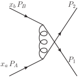
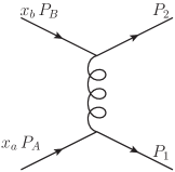
Figure 2: Unpolarized scattering amplitudes for the qqqq𝑞𝑞𝑞𝑞qq\rightarrow qq subprocess. From left the right, the scattering amplitude is provided for the t𝑡t- and u𝑢u-channel processes.

We start with the partonic subprocesses that involve four quarks, such as qqqq𝑞𝑞𝑞𝑞qq\to qq. In Tab. 1, we organize each of the four quark subprocesses into a color basis. The color basis operators acting on particles i𝑖i and j𝑗j are denoted as Γn,ijsubscriptΓ𝑛𝑖𝑗\Gamma_{n,ij} which are used to generate the hard and soft matrices. For the four quark interactions, two operators, n=1,2𝑛12n=1,2, are required to span the color space. As seen in the table, this results in 12 total color matrices. Using the fact that hard function for the unpolarized case is invariant under the charge conjugation, the bottom row can easily be computed from the top row. Furthermore, once the hard matrices have been calculated for the first column, crossing symmetry can be applied in order to obtain the hard color matrices for the second and third column. It is then only necessary to explicitly calculate the hard matrices for the subprocesses associated with the color basis Γn,31Γn,42subscriptΓ𝑛31subscriptΓ𝑛42\Gamma_{n,31}\Gamma_{n,42}.

12 \rightarrow 34 Color Basis 12 \rightarrow 34 Color Basis 12 \rightarrow 34 Color Basis
qqqq𝑞superscript𝑞𝑞superscript𝑞qq^{\prime}\rightarrow qq^{\prime} qq¯qq¯𝑞¯𝑞superscript𝑞superscript¯𝑞q\bar{q}\rightarrow q^{\prime}\bar{q}^{\prime} qq¯q¯q𝑞superscript¯𝑞superscript¯𝑞𝑞q\bar{q}^{\prime}\rightarrow\bar{q}^{\prime}q
qqqq𝑞superscript𝑞superscript𝑞𝑞qq^{\prime}\rightarrow q^{\prime}q Γn,31Γn,42subscriptΓ𝑛31subscriptΓ𝑛42\Gamma_{n,31}\Gamma_{n,42} qq¯qq¯𝑞superscript¯𝑞𝑞superscript¯𝑞q\bar{q}^{\prime}\rightarrow q\bar{q}^{\prime} Γn,21Γn,34subscriptΓ𝑛21subscriptΓ𝑛34\Gamma_{n,21}\Gamma_{n,34} qq¯q¯q𝑞¯𝑞superscript¯𝑞superscript𝑞q\bar{q}\rightarrow\bar{q}^{\prime}q^{\prime} Γn,41Γn,23subscriptΓ𝑛41subscriptΓ𝑛23\Gamma_{n,41}\Gamma_{n,23}
qqqq𝑞superscript𝑞𝑞𝑞qq^{\prime}\rightarrow qq qq¯qq¯𝑞¯𝑞𝑞¯𝑞q\bar{q}\rightarrow q\bar{q} qq¯q¯q𝑞¯𝑞¯𝑞𝑞q\bar{q}\rightarrow\bar{q}q
q¯q¯q¯q¯¯𝑞superscript¯𝑞¯𝑞superscript¯𝑞\bar{q}\bar{q}^{\prime}\rightarrow\bar{q}\bar{q}^{\prime} q¯qq¯q¯𝑞𝑞superscript¯𝑞superscript𝑞\bar{q}q\rightarrow\bar{q}^{\prime}q^{\prime} q¯qqq¯¯𝑞superscript𝑞superscript𝑞¯𝑞\bar{q}q^{\prime}\rightarrow q^{\prime}\bar{q}
q¯q¯q¯q¯¯𝑞superscript¯𝑞superscript¯𝑞¯𝑞\bar{q}\bar{q}^{\prime}\rightarrow\bar{q}^{\prime}\bar{q} Γn,13Γn,24subscriptΓ𝑛13subscriptΓ𝑛24\Gamma_{n,13}\Gamma_{n,24} q¯qq¯q¯𝑞superscript𝑞¯𝑞superscript𝑞\bar{q}q^{\prime}\rightarrow\bar{q}q^{\prime} Γn,12Γn,43subscriptΓ𝑛12subscriptΓ𝑛43\Gamma_{n,12}\Gamma_{n,43} q¯qqq¯¯𝑞𝑞superscript𝑞superscript¯𝑞\bar{q}q\rightarrow q^{\prime}\bar{q}^{\prime} Γn,14Γn,32subscriptΓ𝑛14subscriptΓ𝑛32\Gamma_{n,14}\Gamma_{n,32}
q¯q¯q¯q¯¯𝑞superscript¯𝑞¯𝑞¯𝑞\bar{q}\bar{q}^{\prime}\rightarrow\bar{q}\bar{q} q¯qq¯q¯𝑞𝑞¯𝑞𝑞\bar{q}q\rightarrow\bar{q}q q¯qqq¯¯𝑞𝑞𝑞¯𝑞\bar{q}q\rightarrow q\bar{q}
Table 1: The choice of basis for each of the four quark subprocesses. Γn,ijsubscriptΓ𝑛𝑖𝑗\Gamma_{n,ij} are operators in color space which join the fermion lines i𝑖i and j𝑗j. For the four quark subprocesses, two operators, Γ1,ijsubscriptΓ1𝑖𝑗\Gamma_{1,ij} and Γ2,ijsubscriptΓ2𝑖𝑗\Gamma_{2,ij}, are required to span the color space.

For our calculation, we follow the conventions used in Refs. Liu:2014oog ; Kelley:2010fn to choose Γ1,ij=(ta)ijsubscriptΓ1𝑖𝑗subscriptsuperscript𝑡𝑎𝑖𝑗\Gamma_{1,ij}=(t^{a})_{ij} and Γ2,ij=δijsubscriptΓ2𝑖𝑗subscript𝛿𝑖𝑗\Gamma_{2,ij}=\delta_{ij}, so that the color basis is spanned by the orthogonal basis

θ1=(ta)ij(ta)kl,θ2=δijδkl,formulae-sequencesubscript𝜃1subscriptsuperscript𝑡𝑎𝑖𝑗subscriptsuperscript𝑡𝑎𝑘𝑙subscript𝜃2subscript𝛿𝑖𝑗subscript𝛿𝑘𝑙\displaystyle\theta_{1}=(t^{a})_{ij}(t^{a})_{kl}\,,\qquad\theta_{2}=\delta_{ij}\delta_{kl}\,, (21)
θ1=(ta)ji(ta)lk,θ2=δjiδlk.formulae-sequencesuperscriptsubscript𝜃1subscriptsuperscript𝑡𝑎𝑗𝑖subscriptsuperscript𝑡𝑎𝑙𝑘superscriptsubscript𝜃2subscript𝛿𝑗𝑖subscript𝛿𝑙𝑘\displaystyle\theta_{1}^{\dagger}=(t^{a})_{ji}(t^{a})_{lk}\,,\qquad\theta_{2}^{\dagger}=\delta_{ji}\delta_{lk}\,. (22)

We note that other bases have been used in the literature Moult:2015aoa . We now explicitly perform the calculation for the qqqq𝑞superscript𝑞𝑞superscript𝑞qq^{\prime}\rightarrow qq^{\prime}, qqqq𝑞superscript𝑞superscript𝑞𝑞qq^{\prime}\rightarrow q^{\prime}q, and qqqq𝑞𝑞𝑞𝑞qq\rightarrow qq subprocesses. For these subprocesses, we can write

=tkin(tb)31(tb)42+ukin(tb)32(tb)41superscriptsubscript𝑡kinsubscriptsuperscript𝑡𝑏31subscriptsuperscript𝑡𝑏42superscriptsubscript𝑢kinsubscriptsuperscript𝑡𝑏32subscriptsuperscript𝑡𝑏41\displaystyle\mathcal{M}=\mathcal{M}_{t}^{\rm kin}\left(t^{b}\right)_{31}\left(t^{b}\right)_{42}+\mathcal{M}_{u}^{\rm kin}\left(t^{b}\right)_{32}\left(t^{b}\right)_{41}\, (23)

where we have suppressed the abcd𝑎𝑏𝑐𝑑ab\rightarrow cd subprocess label. The subscript in the \mathcal{M} terms denotes the relevant Mandelstam variable (t^^𝑡\hat{t} or u^^𝑢\hat{u}) for the channel that contributes to the subprocess as shown in the Fig. 2. To arrive at this expressions, we have separated the color parts from the kinematic parts (denoted with the superscript kinkin\rm{kin}). These kinematic scattering amplitudes are defined by

tkin={gs2t^u¯(P1)γμu(xaPA)u¯(P2)γμu(xbPB)abcd=qqqq0forabcd=qqqqgs2t^u¯(P1)γμu(xaPA)u¯(P2)γμu(xbPB)abcd=qqqq,superscriptsubscript𝑡kincasessuperscriptsubscript𝑔𝑠2^𝑡¯𝑢subscript𝑃1superscript𝛾𝜇𝑢subscript𝑥𝑎subscript𝑃𝐴¯𝑢subscript𝑃2subscript𝛾𝜇𝑢subscript𝑥𝑏subscript𝑃𝐵𝑎𝑏𝑐𝑑𝑞superscript𝑞𝑞superscript𝑞0for𝑎𝑏𝑐𝑑𝑞superscript𝑞superscript𝑞𝑞superscriptsubscript𝑔𝑠2^𝑡¯𝑢subscript𝑃1superscript𝛾𝜇𝑢subscript𝑥𝑎subscript𝑃𝐴¯𝑢subscript𝑃2subscript𝛾𝜇𝑢subscript𝑥𝑏subscript𝑃𝐵𝑎𝑏𝑐𝑑𝑞𝑞𝑞𝑞\displaystyle\mathcal{M}_{t}^{\rm kin}=\begin{cases}-\dfrac{g_{s}^{2}}{\hat{t}}\bar{u}(P_{1})\gamma^{\mu}u(x_{a}\,P_{A})\bar{u}(P_{2})\gamma_{\mu}u(x_{b}\,P_{B})&\hskip 5.69046pt\qquad\quad\hskip 2.84544ptab\rightarrow cd=qq^{\prime}\rightarrow qq^{\prime}\\ 0&\hskip 5.69046pt\textrm{for}\qquad ab\rightarrow cd=qq^{\prime}\rightarrow q^{\prime}q\\ -\dfrac{g_{s}^{2}}{\hat{t}}\bar{u}(P_{1})\gamma^{\mu}u(x_{a}\,P_{A})\bar{u}(P_{2})\gamma_{\mu}u(x_{b}\,P_{B})&\hskip 5.69046pt\qquad\quad\hskip 2.84544ptab\rightarrow cd=qq\rightarrow qq\,,\end{cases} (24)
ukin={0abcd=qqqqgs2u^u¯(P2)γμu(xaPA)u¯(P1)γμu(xbPB)forabcd=qqqqgs2u^u¯(P2)γμu(xaPA)u¯(P1)γμu(xbPB)abcd=qqqq.superscriptsubscript𝑢kincases0𝑎𝑏𝑐𝑑𝑞superscript𝑞𝑞superscript𝑞superscriptsubscript𝑔𝑠2^𝑢¯𝑢subscript𝑃2superscript𝛾𝜇𝑢subscript𝑥𝑎subscript𝑃𝐴¯𝑢subscript𝑃1subscript𝛾𝜇𝑢subscript𝑥𝑏subscript𝑃𝐵for𝑎𝑏𝑐𝑑𝑞superscript𝑞superscript𝑞𝑞superscriptsubscript𝑔𝑠2^𝑢¯𝑢subscript𝑃2superscript𝛾𝜇𝑢subscript𝑥𝑎subscript𝑃𝐴¯𝑢subscript𝑃1subscript𝛾𝜇𝑢subscript𝑥𝑏subscript𝑃𝐵𝑎𝑏𝑐𝑑𝑞𝑞𝑞𝑞\displaystyle\mathcal{M}_{u}^{\rm kin}=\begin{cases}0&\hskip 5.69046pt\qquad\quad\hskip 1.42271ptab\rightarrow cd=qq^{\prime}\rightarrow qq^{\prime}\\ -\dfrac{g_{s}^{2}}{\hat{u}}\bar{u}(P_{2})\gamma^{\mu}u(x_{a}\,P_{A})\bar{u}(P_{1})\gamma_{\mu}u(x_{b}\,P_{B})&\hskip 5.69046pt\textrm{for}\qquad ab\rightarrow cd=qq^{\prime}\rightarrow q^{\prime}q\\ \dfrac{g_{s}^{2}}{\hat{u}}\bar{u}(P_{2})\gamma^{\mu}u(x_{a}\,P_{A})\bar{u}(P_{1})\gamma_{\mu}u(x_{b}\,P_{B})&\hskip 5.69046pt\qquad\quad\hskip 1.42271ptab\rightarrow cd=qq\rightarrow qq\,.\end{cases} (25)

We can now decompose these scattering amplitudes in color space as

=1θ1+2θ2=1θ1+2θ2,formulae-sequencesubscript1subscript𝜃1subscript2subscript𝜃2superscriptsuperscriptsubscript1superscriptsubscript𝜃1superscriptsubscript2superscriptsubscript𝜃2\displaystyle\mathcal{M}=\mathcal{M}_{1}\,\theta_{1}+\mathcal{M}_{2}\,\theta_{2}\qquad\mathcal{M}^{\dagger}=\mathcal{M}_{1}^{\dagger}\,\theta_{1}^{\dagger}+\mathcal{M}_{2}^{\dagger}\,\theta_{2}^{\dagger}\,, (26)

where

1=Tr[θ1]Tr[θ1θ1]2=Tr[θ2]Tr[θ2θ2]1=Tr[θ1]Tr[θ1θ1]2=Tr[θ2]Tr[θ2θ2].formulae-sequencesubscript1Trdelimited-[]superscriptsubscript𝜃1Trdelimited-[]subscript𝜃1superscriptsubscript𝜃1formulae-sequencesubscript2Trdelimited-[]superscriptsubscript𝜃2Trdelimited-[]subscript𝜃2superscriptsubscript𝜃2formulae-sequencesuperscriptsubscript1Trdelimited-[]superscriptsubscript𝜃1Trdelimited-[]subscript𝜃1superscriptsubscript𝜃1superscriptsubscript2Trdelimited-[]superscriptsubscript𝜃2Trdelimited-[]subscript𝜃2superscriptsubscript𝜃2\displaystyle\mathcal{M}_{1}=\frac{\hbox{Tr}\left[\mathcal{M}\theta_{1}^{\dagger}\right]}{\hbox{Tr}\left[\theta_{1}\theta_{1}^{\dagger}\right]}\,\qquad\mathcal{M}_{2}=\frac{\hbox{Tr}\left[\mathcal{M}\theta_{2}^{\dagger}\right]}{\hbox{Tr}\left[\theta_{2}\theta_{2}^{\dagger}\right]}\,\qquad\mathcal{M}_{1}^{\dagger}=\frac{\hbox{Tr}\left[\mathcal{M}^{\dagger}\theta_{1}\right]}{\hbox{Tr}\left[\theta_{1}\theta_{1}^{\dagger}\right]}\,\qquad\mathcal{M}_{2}^{\dagger}=\frac{\hbox{Tr}\left[\mathcal{M}^{\dagger}\theta_{2}\right]}{\hbox{Tr}\left[\theta_{2}\theta_{2}^{\dagger}\right]}\,. (27)

To obtain the expressions in Eq. (27), we have exploited the orthogonality of our chosen color basis in Eqs. (21) and (22). Then we will have ||2superscript2|\mathcal{M}|^{2} as

||2=Tr[𝑯abcd𝑺abcd],superscript2Trdelimited-[]subscript𝑯𝑎𝑏𝑐𝑑subscript𝑺𝑎𝑏𝑐𝑑\displaystyle|\mathcal{M}|^{2}=\hbox{Tr}\left[\bm{H}_{ab\rightarrow cd}\cdot\bm{S}_{ab\rightarrow cd}\right]\,, (28)

where the hard matrix is given by

𝑯abcd=[|1|21221|2|2],subscript𝑯𝑎𝑏𝑐𝑑matrixsuperscriptsubscript12subscript1superscriptsubscript2subscript2superscriptsubscript1superscriptsubscript22\displaystyle\bm{H}_{ab\rightarrow cd}=\begin{bmatrix}|\mathcal{M}_{1}|^{2}&\mathcal{M}_{1}\mathcal{M}_{2}^{\dagger}\\ \mathcal{M}_{2}\mathcal{M}_{1}^{\dagger}&|\mathcal{M}_{2}|^{2}\end{bmatrix}\,, (29)

and the leading order soft matrix as

𝑺abcd=[Tr[θ1θ1]Tr[θ1θ2]Tr[θ2θ1]Tr[θ2θ2]]=[12NcCF00Nc2].subscript𝑺𝑎𝑏𝑐𝑑matrixTrdelimited-[]subscript𝜃1superscriptsubscript𝜃1Trdelimited-[]subscript𝜃1superscriptsubscript𝜃2Trdelimited-[]subscript𝜃2superscriptsubscript𝜃1Trdelimited-[]subscript𝜃2superscriptsubscript𝜃2matrix12subscript𝑁𝑐subscript𝐶𝐹00superscriptsubscript𝑁𝑐2\displaystyle\bm{S}_{ab\rightarrow cd}=\begin{bmatrix}\hbox{Tr}\left[\theta_{1}\theta_{1}^{\dagger}\right]&\hbox{Tr}\left[\theta_{1}\theta_{2}^{\dagger}\right]\\ \hbox{Tr}\left[\theta_{2}\theta_{1}^{\dagger}\right]&\hbox{Tr}\left[\theta_{2}\theta_{2}^{\dagger}\right]\end{bmatrix}=\begin{bmatrix}\frac{1}{2}N_{c}C_{F}&0\\ 0&N_{c}^{2}\end{bmatrix}\,. (30)

The hard matrices of the four quark processes in Γ31Γ42subscriptΓ31subscriptΓ42\Gamma_{31}\Gamma_{42} color basis in Tab. 1 are given by

𝑯qqqq=subscript𝑯𝑞superscript𝑞𝑞superscript𝑞absent\displaystyle\bm{H}_{qq^{\prime}\rightarrow qq^{\prime}}= 8gs4(s^2+u^2)t^2[1000],8superscriptsubscript𝑔𝑠4superscript^𝑠2superscript^𝑢2superscript^𝑡2matrix1000\displaystyle\frac{8g_{s}^{4}\left(\hat{s}^{2}+\hat{u}^{2}\right)}{\hat{t}^{2}}\begin{bmatrix}1&0\\ 0&0\\ \end{bmatrix}\,, (31)
𝑯qqqq=subscript𝑯𝑞superscript𝑞superscript𝑞𝑞absent\displaystyle\bm{H}_{qq^{\prime}\rightarrow q^{\prime}q}= 8gs4(s^2+t^2)u^2CA2[1CFCFCF2],8superscriptsubscript𝑔𝑠4superscript^𝑠2superscript^𝑡2superscript^𝑢2superscriptsubscript𝐶𝐴2matrix1subscript𝐶𝐹subscript𝐶𝐹superscriptsubscript𝐶𝐹2\displaystyle\frac{8g_{s}^{4}\left(\hat{s}^{2}+\hat{t}^{2}\right)}{\hat{u}^{2}C_{A}^{2}}\begin{bmatrix}1&-C_{F}\\ -C_{F}&C_{F}^{2}\\ \end{bmatrix}\,, (32)
𝑯qqqq=8gs4t^2u^2Nc2[t^4+s^2t^22Ncs^2u^t^+Nc2u^4+Nc2s^2u^2CFt^(t^3+s^2t^Ncs^2u^)CFt^(t^3+s^2t^Ncs^2u^)CF2t^2(s^2+t^2)].subscript𝑯𝑞𝑞𝑞𝑞8superscriptsubscript𝑔𝑠4superscript^𝑡2superscript^𝑢2superscriptsubscript𝑁𝑐2matrixsuperscript^𝑡4superscript^𝑠2superscript^𝑡22subscript𝑁𝑐superscript^𝑠2^𝑢^𝑡superscriptsubscript𝑁𝑐2superscript^𝑢4superscriptsubscript𝑁𝑐2superscript^𝑠2superscript^𝑢2subscript𝐶𝐹^𝑡superscript^𝑡3superscript^𝑠2^𝑡subscript𝑁𝑐superscript^𝑠2^𝑢subscript𝐶𝐹^𝑡superscript^𝑡3superscript^𝑠2^𝑡subscript𝑁𝑐superscript^𝑠2^𝑢superscriptsubscript𝐶𝐹2superscript^𝑡2superscript^𝑠2superscript^𝑡2\displaystyle\bm{H}_{qq\rightarrow qq}=\frac{8g_{s}^{4}}{\hat{t}^{2}\hat{u}^{2}N_{c}^{2}}\begin{bmatrix}\hat{t}^{4}+\hat{s}^{2}\hat{t}^{2}-2N_{c}\hat{s}^{2}\hat{u}\hat{t}+N_{c}^{2}\hat{u}^{4}+N_{c}^{2}\hat{s}^{2}\hat{u}^{2}&-C_{F}\hat{t}\left(\hat{t}^{3}+\hat{s}^{2}\hat{t}-N_{c}\hat{s}^{2}\hat{u}\right)\\ -C_{F}\hat{t}\left(\hat{t}^{3}+\hat{s}^{2}\hat{t}-N_{c}\hat{s}^{2}\hat{u}\right)&C_{F}^{2}\hat{t}^{2}\left(\hat{s}^{2}+\hat{t}^{2}\right)\\ \end{bmatrix}\,. (33)

We find these results to be consistent with the expressions in Kelley:2010fn . The remaining hard functions can be obtained from crossing symmetries.

III.1.2 Two quarks and two gluon subprocesses

12 \rightarrow 34 Basis 12 \rightarrow 34 Basis 12 \rightarrow 34 Basis 12 \rightarrow 34 Basis 12 \rightarrow 34 Basis 12 \rightarrow 34 Basis
qq¯gg𝑞¯𝑞𝑔𝑔q\bar{q}\rightarrow gg Γn,21absuperscriptsubscriptΓ𝑛21𝑎𝑏\Gamma_{n,21}^{ab} qggq𝑞𝑔𝑔𝑞qg\rightarrow gq Γn,41absuperscriptsubscriptΓ𝑛41𝑎𝑏\Gamma_{n,41}^{ab} qgqg𝑞𝑔𝑞𝑔qg\rightarrow qg Γn,31absuperscriptsubscriptΓ𝑛31𝑎𝑏\Gamma_{n,31}^{ab} gqgq𝑔𝑞𝑔𝑞gq\rightarrow gq Γn,42absuperscriptsubscriptΓ𝑛42𝑎𝑏\Gamma_{n,42}^{ab} gqqg𝑔𝑞𝑞𝑔gq\rightarrow qg Γn,32absuperscriptsubscriptΓ𝑛32𝑎𝑏\Gamma_{n,32}^{ab} ggqq¯𝑔𝑔𝑞¯𝑞gg\rightarrow q\bar{q} Γn,43absuperscriptsubscriptΓ𝑛43𝑎𝑏\Gamma_{n,43}^{ab}
q¯gq¯g¯𝑞𝑔¯𝑞𝑔\bar{q}g\rightarrow\bar{q}g Γn,21absuperscriptsubscriptΓ𝑛21𝑎𝑏\Gamma_{n,21}^{ab} q¯ggq¯¯𝑞𝑔𝑔¯𝑞\bar{q}g\rightarrow g\bar{q} Γn,41absuperscriptsubscriptΓ𝑛41𝑎𝑏\Gamma_{n,41}^{ab} q¯qgg¯𝑞𝑞𝑔𝑔\bar{q}q\rightarrow gg Γn,31absuperscriptsubscriptΓ𝑛31𝑎𝑏\Gamma_{n,31}^{ab} ggq¯q𝑔𝑔¯𝑞𝑞gg\rightarrow\bar{q}q Γn,42absuperscriptsubscriptΓ𝑛42𝑎𝑏\Gamma_{n,42}^{ab} gq¯q¯g𝑔¯𝑞¯𝑞𝑔g\bar{q}\rightarrow\bar{q}g Γn,32absuperscriptsubscriptΓ𝑛32𝑎𝑏\Gamma_{n,32}^{ab} gq¯gq¯𝑔¯𝑞𝑔¯𝑞g\bar{q}\rightarrow g\bar{q} Γn,43absuperscriptsubscriptΓ𝑛43𝑎𝑏\Gamma_{n,43}^{ab}
Table 2: The choice of basis for each of two quark two gluon subprocesses. Three operators Γ1,ijabsuperscriptsubscriptΓ1𝑖𝑗𝑎𝑏\Gamma_{1,ij}^{ab},Γ2,ijabsuperscriptsubscriptΓ2𝑖𝑗𝑎𝑏\Gamma_{2,ij}^{ab},Γ3,ijabsuperscriptsubscriptΓ3𝑖𝑗𝑎𝑏\Gamma_{3,ij}^{ab} are required to span the color space for each subprocess.

In Tab. 2, we provide a list of subprocesses involving two quarks and two gluons with the color basis operators Γn,ijabsuperscriptsubscriptΓ𝑛𝑖𝑗𝑎𝑏\Gamma_{n,ij}^{ab}. For the two quark and two gluon interactions, three operators, n=1,2,3𝑛123n=1,2,3, are required to span the color space. A convenient choice for the computation is the set of orthogonal operators (primed),

Γ1,ijab=δab2Ncδij,Γ2,ijab=12dabctijc,Γ3,ijab=12fabctijc,formulae-sequencesuperscriptsubscriptsuperscriptΓ𝑎𝑏1𝑖𝑗superscript𝛿𝑎𝑏2subscript𝑁𝑐subscript𝛿𝑖𝑗formulae-sequencesuperscriptsubscriptsuperscriptΓ𝑎𝑏2𝑖𝑗12superscript𝑑𝑎𝑏𝑐subscriptsuperscript𝑡𝑐𝑖𝑗superscriptsubscriptsuperscriptΓ𝑎𝑏3𝑖𝑗12superscript𝑓𝑎𝑏𝑐subscriptsuperscript𝑡𝑐𝑖𝑗\displaystyle{\Gamma^{ab}_{1,ij}}^{\prime}=\frac{\delta^{ab}}{2N_{c}}\delta_{ij}\,,\qquad{\Gamma^{ab}_{2,ij}}^{\prime}=\frac{1}{2}d^{abc}t^{c}_{ij}\,,\qquad{\Gamma^{ab}_{3,ij}}^{\prime}=\frac{1}{2}f^{abc}t^{c}_{ij}\,, (34)

which has the corresponding orthogonal basis,

θ1=δab2Ncδij,θ2=12dabctijc,θ3=12fabctijc.formulae-sequencesuperscriptsubscript𝜃1superscript𝛿𝑎𝑏2subscript𝑁𝑐subscript𝛿𝑖𝑗formulae-sequencesuperscriptsubscript𝜃212superscript𝑑𝑎𝑏𝑐subscriptsuperscript𝑡𝑐𝑖𝑗superscriptsubscript𝜃312superscript𝑓𝑎𝑏𝑐subscriptsuperscript𝑡𝑐𝑖𝑗\displaystyle\theta_{1}^{\prime}=\frac{\delta^{ab}}{2N_{c}}\delta_{ij}\,,\qquad\theta_{2}^{\prime}=\frac{1}{2}d^{abc}t^{c}_{ij}\,,\qquad\theta_{3}^{\prime}=\frac{1}{2}f^{abc}t^{c}_{ij}\,. (35)

At the same time, we find that the final expressions for the hard matrices take a simpler form when one uses the non-orthogonal basis used in Refs. Liu:2014oog ; Kelley:2010fn ; Moult:2015aoa by defining the basis operators to be (unprimed)

Γ1,ijab=(tatb)ij,Γ2,ijab=(tbta)ij,Γ3,ijab=δijδab.formulae-sequencesubscriptsuperscriptΓ𝑎𝑏1𝑖𝑗subscriptsuperscript𝑡𝑎superscript𝑡𝑏𝑖𝑗formulae-sequencesubscriptsuperscriptΓ𝑎𝑏2𝑖𝑗subscriptsuperscript𝑡𝑏superscript𝑡𝑎𝑖𝑗subscriptsuperscriptΓ𝑎𝑏3𝑖𝑗subscript𝛿𝑖𝑗superscript𝛿𝑎𝑏\displaystyle\Gamma^{ab}_{1,ij}=(t^{a}t^{b})_{ij}\,,\qquad\Gamma^{ab}_{2,ij}=(t^{b}t^{a})_{ij}\,,\qquad\Gamma^{ab}_{3,ij}=\delta_{ij}\delta^{ab}\,. (36)

The corresponding basis is given by

θ1=(tatb)ij,θ2=(tbta)ij,θ3=δijδab.formulae-sequencesubscript𝜃1subscriptsuperscript𝑡𝑎superscript𝑡𝑏𝑖𝑗formulae-sequencesubscript𝜃2subscriptsuperscript𝑡𝑏superscript𝑡𝑎𝑖𝑗subscript𝜃3subscript𝛿𝑖𝑗superscript𝛿𝑎𝑏\displaystyle\theta_{1}=(t^{a}t^{b})_{ij}\,,\qquad\theta_{2}=(t^{b}t^{a})_{ij}\,,\qquad\theta_{3}=\delta_{ij}\delta^{ab}\,. (37)

We note that the normalization of θ3subscript𝜃3\theta_{3} in Moult:2015aoa differs from the normalization of Refs. Liu:2014oog ; Kelley:2010fn by a factor of 2. For the choice of basis in Eq. (37), the LO soft matrix is given by

𝑺abcd=[Tr[θ1θ1]Tr[θ1θ2]Tr[θ1θ3]Tr[θ2θ1]Tr[θ2θ2]Tr[θ2θ3]Tr[θ3θ1]Tr[θ3θ2]Tr[θ3θ3]]=[NcCF2CF2NcCFCF2NcCF2NcCFNcCFNcCF2Nc2CF].subscript𝑺𝑎𝑏𝑐𝑑matrixTrdelimited-[]subscript𝜃1superscriptsubscript𝜃1Trdelimited-[]subscript𝜃1superscriptsubscript𝜃2Trdelimited-[]subscript𝜃1superscriptsubscript𝜃3Trdelimited-[]subscript𝜃2superscriptsubscript𝜃1Trdelimited-[]subscript𝜃2superscriptsubscript𝜃2Trdelimited-[]subscript𝜃2superscriptsubscript𝜃3Trdelimited-[]subscript𝜃3superscriptsubscript𝜃1Trdelimited-[]subscript𝜃3superscriptsubscript𝜃2Trdelimited-[]subscript𝜃3superscriptsubscript𝜃3matrixsubscript𝑁𝑐superscriptsubscript𝐶𝐹2subscript𝐶𝐹2subscript𝑁𝑐subscript𝐶𝐹subscript𝐶𝐹2subscript𝑁𝑐superscriptsubscript𝐶𝐹2subscript𝑁𝑐subscript𝐶𝐹subscript𝑁𝑐subscript𝐶𝐹subscript𝑁𝑐subscript𝐶𝐹2superscriptsubscript𝑁𝑐2subscript𝐶𝐹\displaystyle\bm{S}_{ab\rightarrow cd}=\begin{bmatrix}\hbox{Tr}\left[\theta_{1}\theta_{1}^{\dagger}\right]&\hbox{Tr}\left[\theta_{1}\theta_{2}^{\dagger}\right]&\hbox{Tr}\left[\theta_{1}\theta_{3}^{\dagger}\right]\\ \hbox{Tr}\left[\theta_{2}\theta_{1}^{\dagger}\right]&\hbox{Tr}\left[\theta_{2}\theta_{2}^{\dagger}\right]&\hbox{Tr}\left[\theta_{2}\theta_{3}^{\dagger}\right]\\ \hbox{Tr}\left[\theta_{3}\theta_{1}^{\dagger}\right]&\hbox{Tr}\left[\theta_{3}\theta_{2}^{\dagger}\right]&\hbox{Tr}\left[\theta_{3}\theta_{3}^{\dagger}\right]\end{bmatrix}=\begin{bmatrix}N_{c}C_{F}^{2}&-\frac{C_{F}}{2}&N_{c}C_{F}\\ -\frac{C_{F}}{2}&N_{c}C_{F}^{2}&N_{c}C_{F}\\ N_{c}C_{F}&N_{c}C_{F}&2N_{c}^{2}C_{F}\\ \end{bmatrix}\,. (38)

In order to exploit the orthogonality condition of the primed basis in Eq. (35), but still provide a simple expression for the hard matrices using the unprimed basis in Eq. (37), we first compute the hard matrices in the primed basis then obtain the results in the unprimed basis using the relation

𝑯abcd=𝑹𝑯abcd𝑹,where𝑹=[1111112Nc00]1.formulae-sequencesubscript𝑯𝑎𝑏𝑐𝑑superscript𝑹superscriptsubscript𝑯𝑎𝑏𝑐𝑑𝑹where𝑹superscriptmatrix1111112subscript𝑁𝑐001\displaystyle\bm{H}_{ab\rightarrow cd}=\bm{R}^{\dagger}\,\bm{H}_{ab\rightarrow cd}^{\prime}\,\bm{R}\,,\qquad\text{where}\quad\bm{R}=\begin{bmatrix}1&1&-1\\ 1&1&1\\ 2N_{c}&0&0\end{bmatrix}^{-1}\,. (39)

We now perform the calculation for the hard matrices for the qq¯gg𝑞¯𝑞𝑔𝑔q\bar{q}\rightarrow gg process in the primed orthogonal basis. The scattering amplitude for this subprocess can be written in color space as

=M1θ1+M2θ2+M3θ3=M1θ1+M2θ2+M3θ3formulae-sequencesubscript𝑀1superscriptsubscript𝜃1subscript𝑀2superscriptsubscript𝜃2subscript𝑀3superscriptsubscript𝜃3superscriptsuperscriptsubscript𝑀1superscriptsuperscriptsubscript𝜃1superscriptsubscript𝑀2superscriptsuperscriptsubscript𝜃2superscriptsubscript𝑀3superscriptsuperscriptsubscript𝜃3\displaystyle\mathcal{M}=M_{1}\theta_{1}^{\prime}+M_{2}\theta_{2}^{\prime}+M_{3}\theta_{3}^{\prime}\qquad\mathcal{M}^{\dagger}=M_{1}^{\dagger}{\theta_{1}^{\prime}}^{\dagger}+M_{2}^{\dagger}{\theta_{2}^{\prime}}^{\dagger}+M_{3}^{\dagger}{\theta_{3}^{\prime}}^{\dagger} (40)

where

1=Tr[θ1]Tr[θ1θ1]2=Tr[θ2]Tr[θ2θ2],3=Tr[θ3]Tr[θ3θ3],formulae-sequencesubscript1Trdelimited-[]superscriptsuperscriptsubscript𝜃1Trdelimited-[]superscriptsubscript𝜃1superscriptsuperscriptsubscript𝜃1formulae-sequencesubscript2Trdelimited-[]superscriptsuperscriptsubscript𝜃2Trdelimited-[]superscriptsubscript𝜃2superscriptsuperscriptsubscript𝜃2subscript3Trdelimited-[]superscriptsuperscriptsubscript𝜃3Trdelimited-[]superscriptsubscript𝜃3superscriptsuperscriptsubscript𝜃3\displaystyle\mathcal{M}_{1}=\frac{\hbox{Tr}\left[\mathcal{M}{\theta_{1}^{\prime}}^{\dagger}\right]}{\hbox{Tr}\left[{\theta_{1}^{\prime}}{\theta_{1}^{\prime}}^{\dagger}\right]}\,\qquad\mathcal{M}_{2}=\frac{\hbox{Tr}\left[\mathcal{M}{\theta_{2}^{\prime}}^{\dagger}\right]}{\hbox{Tr}\left[{\theta_{2}^{\prime}}{\theta_{2}^{\prime}}^{\dagger}\right]}\,,\qquad\mathcal{M}_{3}=\frac{\hbox{Tr}\left[\mathcal{M}{\theta_{3}^{\prime}}^{\dagger}\right]}{\hbox{Tr}\left[{\theta_{3}^{\prime}}{\theta_{3}^{\prime}}^{\dagger}\right]}\,, (41)
1=Tr[θ1]Tr[θ1θ1]2=Tr[θ2]Tr[θ2θ2],3=Tr[θ3]Tr[θ3θ3].formulae-sequencesuperscriptsubscript1Trdelimited-[]superscriptsuperscriptsubscript𝜃1Trdelimited-[]superscriptsubscript𝜃1superscriptsuperscriptsubscript𝜃1formulae-sequencesuperscriptsubscript2Trdelimited-[]superscriptsuperscriptsubscript𝜃2Trdelimited-[]superscriptsubscript𝜃2superscriptsuperscriptsubscript𝜃2superscriptsubscript3Trdelimited-[]superscriptsuperscriptsubscript𝜃3Trdelimited-[]superscriptsubscript𝜃3superscriptsuperscriptsubscript𝜃3\displaystyle\mathcal{M}_{1}^{\dagger}=\frac{\hbox{Tr}\left[\mathcal{M}^{\dagger}{\theta_{1}^{\prime}}\right]}{\hbox{Tr}\left[{\theta_{1}^{\prime}}{\theta_{1}^{\prime}}^{\dagger}\right]}\,\qquad\mathcal{M}_{2}^{\dagger}=\frac{\hbox{Tr}\left[\mathcal{M}^{\dagger}{\theta_{2}^{\prime}}\right]}{\hbox{Tr}\left[{\theta_{2}^{\prime}}{\theta_{2}^{\prime}}^{\dagger}\right]}\,,\qquad\mathcal{M}_{3}^{\dagger}=\frac{\hbox{Tr}\left[\mathcal{M}^{\dagger}{\theta_{3}^{\prime}}\right]}{\hbox{Tr}\left[{\theta_{3}^{\prime}}{\theta_{3}^{\prime}}^{\dagger}\right]}\,. (42)

The hard matrix in the primed basis can therefore be computed as

𝑯qq¯gg=[M1M1M1M2M1M3M2M1M2M2M2M3M3M1M3M2M3M3].subscriptsuperscript𝑯𝑞¯𝑞𝑔𝑔matrixsubscript𝑀1superscriptsubscript𝑀1subscript𝑀1superscriptsubscript𝑀2subscript𝑀1superscriptsubscript𝑀3subscript𝑀2superscriptsubscript𝑀1subscript𝑀2superscriptsubscript𝑀2subscript𝑀2superscriptsubscript𝑀3subscript𝑀3superscriptsubscript𝑀1subscript𝑀3superscriptsubscript𝑀2subscript𝑀3superscriptsubscript𝑀3\displaystyle\bm{H}^{\prime}_{q\bar{q}\rightarrow gg}=\begin{bmatrix}M_{1}\,M_{1}^{\dagger}&M_{1}\,M_{2}^{\dagger}&M_{1}\,M_{3}^{\dagger}\\ M_{2}\,M_{1}^{\dagger}&M_{2}\,M_{2}^{\dagger}&M_{2}\,M_{3}^{\dagger}\\ M_{3}\,M_{1}^{\dagger}&M_{3}\,M_{2}^{\dagger}&M_{3}\,M_{3}^{\dagger}\\ \end{bmatrix}\,. (43)

Finally, we now use Eq. (39) to obtain the simplified hard functions in the unprimed basis as

𝑯qq¯gg=8gs4(t^2+u^2)s^2[u^t^101t^u^0000].subscript𝑯𝑞¯𝑞𝑔𝑔8superscriptsubscript𝑔𝑠4superscript^𝑡2superscript^𝑢2superscript^𝑠2matrix^𝑢^𝑡101^𝑡^𝑢0000\displaystyle\bm{H}_{q\bar{q}\rightarrow gg}=8g_{s}^{4}\frac{\left(\hat{t}^{2}+\hat{u}^{2}\right)}{\hat{s}^{2}}\begin{bmatrix}\frac{\hat{u}}{\hat{t}}&1&0\\ 1&\frac{\hat{t}}{\hat{u}}&0\\ 0&0&0\\ \end{bmatrix}\,. (44)

The hard matrices for other subprocesses involving two quarks and two gluons, such as qgqg𝑞𝑔𝑞𝑔qg\to qg, can be obtained from this expression using crossing symmetries.

III.1.3 Four gluon subprocesses

For the four gluon subprocesses, gggg𝑔𝑔𝑔𝑔gg\to gg, we follow the work in Refs. Kelley:2010fn ; Liu:2014oog to use the following over-complete basis

θ1=Tr[ta1ta2ta3ta4],subscript𝜃1Trdelimited-[]superscript𝑡subscript𝑎1superscript𝑡subscript𝑎2superscript𝑡subscript𝑎3superscript𝑡subscript𝑎4\displaystyle\theta_{1}=\hbox{Tr}\left[t^{a_{1}}t^{a_{2}}t^{a_{3}}t^{a_{4}}\right]\,,\qquad θ2=Tr[ta1ta2ta4ta3],subscript𝜃2Trdelimited-[]superscript𝑡subscript𝑎1superscript𝑡subscript𝑎2superscript𝑡subscript𝑎4superscript𝑡subscript𝑎3\displaystyle\theta_{2}=\hbox{Tr}\left[t^{a_{1}}t^{a_{2}}t^{a_{4}}t^{a_{3}}\right]\,,\qquad θ3=Tr[ta1ta4ta3ta2],subscript𝜃3Trdelimited-[]superscript𝑡subscript𝑎1superscript𝑡subscript𝑎4superscript𝑡subscript𝑎3superscript𝑡subscript𝑎2\displaystyle\theta_{3}=\hbox{Tr}\left[t^{a_{1}}t^{a_{4}}t^{a_{3}}t^{a_{2}}\right]\,,
θ4=Tr[ta1ta4ta2ta3],subscript𝜃4Trdelimited-[]superscript𝑡subscript𝑎1superscript𝑡subscript𝑎4superscript𝑡subscript𝑎2superscript𝑡subscript𝑎3\displaystyle\theta_{4}=\hbox{Tr}\left[t^{a_{1}}t^{a_{4}}t^{a_{2}}t^{a_{3}}\right]\,,\qquad θ5=Tr[ta1ta3ta4ta2],subscript𝜃5Trdelimited-[]superscript𝑡subscript𝑎1superscript𝑡subscript𝑎3superscript𝑡subscript𝑎4superscript𝑡subscript𝑎2\displaystyle\theta_{5}=\hbox{Tr}\left[t^{a_{1}}t^{a_{3}}t^{a_{4}}t^{a_{2}}\right]\,,\qquad θ6=Tr[ta1ta3ta2ta4],subscript𝜃6Trdelimited-[]superscript𝑡subscript𝑎1superscript𝑡subscript𝑎3superscript𝑡subscript𝑎2superscript𝑡subscript𝑎4\displaystyle\theta_{6}=\hbox{Tr}\left[t^{a_{1}}t^{a_{3}}t^{a_{2}}t^{a_{4}}\right]\,,
θ7=Tr[ta1ta4]Tr[ta2ta3],subscript𝜃7Trdelimited-[]superscript𝑡subscript𝑎1superscript𝑡subscript𝑎4Trdelimited-[]superscript𝑡subscript𝑎2superscript𝑡subscript𝑎3\displaystyle\theta_{7}=\hbox{Tr}\left[t^{a_{1}}t^{a_{4}}\right]\hbox{Tr}\left[t^{a_{2}}t^{a_{3}}\right]\,,\qquad θ8=Tr[ta1ta2]Tr[ta3ta4],subscript𝜃8Trdelimited-[]superscript𝑡subscript𝑎1superscript𝑡subscript𝑎2Trdelimited-[]superscript𝑡subscript𝑎3superscript𝑡subscript𝑎4\displaystyle\theta_{8}=\hbox{Tr}\left[t^{a_{1}}t^{a_{2}}\right]\hbox{Tr}\left[t^{a_{3}}t^{a_{4}}\right]\,,\qquad θ9=Tr[ta1ta3]Tr[ta2ta4].subscript𝜃9Trdelimited-[]superscript𝑡subscript𝑎1superscript𝑡subscript𝑎3Trdelimited-[]superscript𝑡subscript𝑎2superscript𝑡subscript𝑎4\displaystyle\theta_{9}=\hbox{Tr}\left[t^{a_{1}}t^{a_{3}}\right]\hbox{Tr}\left[t^{a_{2}}t^{a_{4}}\right]\,. (45)

We note that a six dimensional basis was chosen in Moult:2015aoa . Using this basis in Eq. (45), one can show that the hard matrix takes the following form

𝑯gggg=2gs4(s^4+t^4+u^4)s^2u^2Nc2CF2[1u^t^1s^t^u^t^s^t^000u^t^u^2t^2u^t^s^u^t^2u^2t^2s^u^t^20001u^t^1s^t^u^t^s^t^000s^t^s^u^t^2s^t^s^2t^2s^u^t^2s^2t^2000u^t^u^2t^2u^t^s^u^t^2u^2t^2s^u^t^2000s^t^s^u^t^2s^t^s^2t^2s^u^t^2s^2t^2000000000000000000000000000000].subscript𝑯𝑔𝑔𝑔𝑔2superscriptsubscript𝑔𝑠4superscript^𝑠4superscript^𝑡4superscript^𝑢4superscript^𝑠2superscript^𝑢2superscriptsubscript𝑁𝑐2superscriptsubscript𝐶𝐹2matrix1^𝑢^𝑡1^𝑠^𝑡^𝑢^𝑡^𝑠^𝑡000^𝑢^𝑡superscript^𝑢2superscript^𝑡2^𝑢^𝑡^𝑠^𝑢superscript^𝑡2superscript^𝑢2superscript^𝑡2^𝑠^𝑢superscript^𝑡20001^𝑢^𝑡1^𝑠^𝑡^𝑢^𝑡^𝑠^𝑡000^𝑠^𝑡^𝑠^𝑢superscript^𝑡2^𝑠^𝑡superscript^𝑠2superscript^𝑡2^𝑠^𝑢superscript^𝑡2superscript^𝑠2superscript^𝑡2000^𝑢^𝑡superscript^𝑢2superscript^𝑡2^𝑢^𝑡^𝑠^𝑢superscript^𝑡2superscript^𝑢2superscript^𝑡2^𝑠^𝑢superscript^𝑡2000^𝑠^𝑡^𝑠^𝑢superscript^𝑡2^𝑠^𝑡superscript^𝑠2superscript^𝑡2^𝑠^𝑢superscript^𝑡2superscript^𝑠2superscript^𝑡2000000000000000000000000000000\displaystyle\bm{H}_{gg\to gg}=\frac{2g_{s}^{4}\left(\hat{s}^{4}+\hat{t}^{4}+\hat{u}^{4}\right)}{\hat{s}^{2}\hat{u}^{2}N_{c}^{2}C_{F}^{2}}\begin{bmatrix}1&\frac{\hat{u}}{\hat{t}}&1&\frac{\hat{s}}{\hat{t}}&\frac{\hat{u}}{\hat{t}}&\frac{\hat{s}}{\hat{t}}&0&0&0\\ \frac{\hat{u}}{\hat{t}}&\frac{\hat{u}^{2}}{\hat{t}^{2}}&\frac{\hat{u}}{\hat{t}}&\frac{\hat{s}\hat{u}}{\hat{t}^{2}}&\frac{\hat{u}^{2}}{\hat{t}^{2}}&\frac{\hat{s}\hat{u}}{\hat{t}^{2}}&0&0&0\\ 1&\frac{\hat{u}}{\hat{t}}&1&\frac{\hat{s}}{\hat{t}}&\frac{\hat{u}}{\hat{t}}&\frac{\hat{s}}{\hat{t}}&0&0&0\\ \frac{\hat{s}}{\hat{t}}&\frac{\hat{s}\hat{u}}{\hat{t}^{2}}&\frac{\hat{s}}{\hat{t}}&\frac{\hat{s}^{2}}{\hat{t}^{2}}&\frac{\hat{s}\hat{u}}{\hat{t}^{2}}&\frac{\hat{s}^{2}}{\hat{t}^{2}}&0&0&0\\ \frac{\hat{u}}{\hat{t}}&\frac{\hat{u}^{2}}{\hat{t}^{2}}&\frac{\hat{u}}{\hat{t}}&\frac{\hat{s}\hat{u}}{\hat{t}^{2}}&\frac{\hat{u}^{2}}{\hat{t}^{2}}&\frac{\hat{s}\hat{u}}{\hat{t}^{2}}&0&0&0\\ \frac{\hat{s}}{\hat{t}}&\frac{\hat{s}\hat{u}}{\hat{t}^{2}}&\frac{\hat{s}}{\hat{t}}&\frac{\hat{s}^{2}}{\hat{t}^{2}}&\frac{\hat{s}\hat{u}}{\hat{t}^{2}}&\frac{\hat{s}^{2}}{\hat{t}^{2}}&0&0&0\\ 0&0&0&0&0&0&0&0&0\\ 0&0&0&0&0&0&0&0&0\\ 0&0&0&0&0&0&0&0&0\\ \end{bmatrix}\,. (46)

The LO soft matrix for this channel is given in Appendix C of Liu:2014oog for this basis as

𝑺gggg=CF8Nc[a0b0c0b0b0b0d0d0e0b0a0b0b0c0b0e0d0b0c0b0a0b0b0b0d0d0e0b0b0b0a0b0c0d0e0d0b0c0b0b0a0b0e0d0d0b0b0b0c0b0a0d0e0d0d0e0d0d0e0d0d0e0e02e02d0d0d0e0d0e0e02d0e0e02e0d0e0d0d0d0e02e02d0e0],subscript𝑺𝑔𝑔𝑔𝑔subscript𝐶𝐹8subscript𝑁𝑐matrixsubscript𝑎0subscript𝑏0subscript𝑐0subscript𝑏0subscript𝑏0subscript𝑏0subscript𝑑0subscript𝑑0subscript𝑒0subscript𝑏0subscript𝑎0subscript𝑏0subscript𝑏0subscript𝑐0subscript𝑏0subscript𝑒0subscript𝑑0subscript𝑏0subscript𝑐0subscript𝑏0subscript𝑎0subscript𝑏0subscript𝑏0subscript𝑏0subscript𝑑0subscript𝑑0subscript𝑒0subscript𝑏0subscript𝑏0subscript𝑏0subscript𝑎0subscript𝑏0subscript𝑐0subscript𝑑0subscript𝑒0subscript𝑑0subscript𝑏0subscript𝑐0subscript𝑏0subscript𝑏0subscript𝑎0subscript𝑏0subscript𝑒0subscript𝑑0subscript𝑑0subscript𝑏0subscript𝑏0subscript𝑏0subscript𝑐0subscript𝑏0subscript𝑎0subscript𝑑0subscript𝑒0subscript𝑑0subscript𝑑0subscript𝑒0subscript𝑑0subscript𝑑0subscript𝑒0subscript𝑑0subscript𝑑0subscript𝑒0superscriptsubscript𝑒02superscriptsubscript𝑒02subscript𝑑0subscript𝑑0subscript𝑑0subscript𝑒0subscript𝑑0subscript𝑒0superscriptsubscript𝑒02subscript𝑑0subscript𝑒0superscriptsubscript𝑒02subscript𝑒0subscript𝑑0subscript𝑒0subscript𝑑0subscript𝑑0subscript𝑑0superscriptsubscript𝑒02superscriptsubscript𝑒02subscript𝑑0subscript𝑒0\displaystyle\bm{S}_{gg\to gg}=\frac{C_{F}}{8N_{c}}\begin{bmatrix}a_{0}&b_{0}&c_{0}&b_{0}&b_{0}&b_{0}&d_{0}&d_{0}&-e_{0}\\ b_{0}&a_{0}&b_{0}&b_{0}&c_{0}&b_{0}&-e_{0}&d_{0}&b_{0}\\ c_{0}&b_{0}&a_{0}&b_{0}&b_{0}&b_{0}&d_{0}&d_{0}&-e_{0}\\ b_{0}&b_{0}&b_{0}&a_{0}&b_{0}&c_{0}&d_{0}&-e_{0}&d_{0}\\ b_{0}&c_{0}&b_{0}&b_{0}&a_{0}&b_{0}&-e_{0}&d_{0}&d_{0}\\ b_{0}&b_{0}&b_{0}&c_{0}&b_{0}&a_{0}&d_{0}&-e_{0}&d_{0}\\ d_{0}&-e_{0}&d_{0}&d_{0}&-e_{0}&d_{0}&d_{0}e_{0}&e_{0}^{2}&e_{0}^{2}\\ d_{0}&d_{0}&d_{0}&-e_{0}&d_{0}&-e_{0}&e_{0}^{2}&d_{0}e_{0}&e_{0}^{2}\\ -e_{0}&d_{0}&-e_{0}&d_{0}&d_{0}&d_{0}&e_{0}^{2}&e_{0}^{2}&d_{0}e_{0}\\ \end{bmatrix}\,, (47)

where a0=Nc43Nc2+3subscript𝑎0superscriptsubscript𝑁𝑐43superscriptsubscript𝑁𝑐23a_{0}=N_{c}^{4}-3N_{c}^{2}+3, b0=3Nc2subscript𝑏03superscriptsubscript𝑁𝑐2b_{0}=3-N_{c}^{2}, c0=3+Nc2subscript𝑐03superscriptsubscript𝑁𝑐2c_{0}=3+N_{c}^{2}, d0=2Nc2CFsubscript𝑑02superscriptsubscript𝑁𝑐2subscript𝐶𝐹d_{0}=2N_{c}^{2}C_{F}, and e0=Ncsubscript𝑒0subscript𝑁𝑐e_{0}=N_{c}.

III.2 Polarized Hard Matrices

As we have emphasized in the previous section, Sivers function is non-universal. The well-known example is the sign change between the Sivers function probed in SIDIS and that in Drell-Yan (DY) process Brodsky:2002rv ; Collins:2002kn ; Boer:2003cm ,

f1Tq(DY)(x,k,μ)=f1Tq(SIDIS)(x,k,μ).superscriptsubscript𝑓1𝑇perpendicular-toabsent𝑞DY𝑥subscript𝑘perpendicular-to𝜇superscriptsubscript𝑓1𝑇perpendicular-toabsent𝑞SIDIS𝑥subscript𝑘perpendicular-to𝜇\displaystyle f_{1T}^{\perp\,q{\rm(DY)}}(x,k_{\perp},\mu)=-f_{1T}^{\perp\,q{\rm(SIDIS)}}(x,k_{\perp},\mu)\,. (48)

Such a sign change can be easily taken care of in describing the Drell-Yan Sivers asymmetry,

dΔσ(S)f1Tq(DY)(x,k,μ)H(Q,μ)=f1Tq(SIDIS)(x,k,μ)[H(Q,μ)],proportional-to𝑑Δ𝜎subscript𝑆perpendicular-tosuperscriptsubscript𝑓1𝑇perpendicular-toabsent𝑞DY𝑥subscript𝑘perpendicular-to𝜇𝐻𝑄𝜇superscriptsubscript𝑓1𝑇perpendicular-toabsent𝑞SIDIS𝑥subscript𝑘perpendicular-to𝜇delimited-[]𝐻𝑄𝜇\displaystyle d\Delta\sigma(S_{\perp})\propto f_{1T}^{\perp\,q{\rm(DY)}}(x,k_{\perp},\mu)H(Q,\mu)=f_{1T}^{\perp\,q{\rm(SIDIS)}}(x,k_{\perp},\mu)\big{[}-H(Q,\mu)\big{]}\,, (49)

where H(Q,μ)𝐻𝑄𝜇H(Q,\mu) is the hard function in the Drell-Yan process, and we have applied Eq. (48) in the second step. In other words, if we use the SIDIS Sivers function in a Drell-Yan process, we shift the minus sign (or the process-dependence) into the hard function.

For the partonic subprocesses in the hadronic dijet production, one has much more complicated process-dependence for the Sivers functions involved. This can be seen from the highly nontrivial gauge link structure which has been derived in Bomhof:2006dp in the definition of the TMD PDFs. Even in these complicated processes, one can incorporate such process-dependence of the Sivers functions into modified hard functions as in Eq. (49Bacchetta:2005rm ; Bomhof:2007su ; Qiu:2007ey ; Vogelsang:2007jk ; Qiu:2007ar . We follow a similar procedure in this section to include this process-dependence of the Sivers functions into the hard functions in the matrix form.

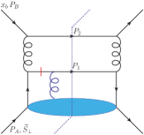
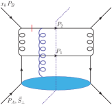
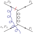
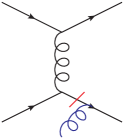
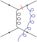
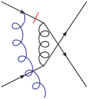
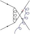
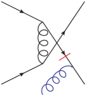
In Fig. 3, we demonstrate the factorization between the Sivers function and modified hard functions. Unlike the unpolarized case, the contributions of the Sivers asymmetry are given by considering the attachment of an additional collinear (to the incoming hadron) gluon to three of the external legs. Such a gluon is part of the gauge link in the definition of the Sivers function, and it is the imaginary part of the Feynman diagram (related to the so-called soft gluonic pole) that contributes to the process-dependence of the Sivers function.

It is important to note that the additional gluon leads to additional complications so that naive crossing symmetry cannot be used to relate one hard function to another, as in the unpolarized case studied above. These complications occur because the contributions to the Sivers asymmetry are only given by attaching the additional gluon to three of the four external legs. Furthermore, since the sign of the interaction (imaginary part) with the external gluon is opposite for quarks and anti-quarks, this sign must also be accounted for when applying crossing symmetry or charge conjugation.
Refer to caption

= Refer to caption Refer to caption Refer to caption ×tj1aCFabsentsubscriptsuperscript𝑡𝑎𝑗1subscript𝐶𝐹\times\dfrac{t^{a}_{j1}}{C_{F}} Refer to caption = Refer to caption Refer to caption Refer to caption ×tj1aCFabsentsubscriptsuperscript𝑡𝑎𝑗1subscript𝐶𝐹\times\dfrac{t^{a}_{j1}}{C_{F}} Refer to caption = Refer to caption Refer to caption Refer to caption ×tj1aCFabsentsubscriptsuperscript𝑡𝑎𝑗1subscript𝐶𝐹\times\dfrac{t^{a}_{j1}}{C_{F}}

Figure 3: A demonstration of the factorization between the Sivers function and the hard function for qqqq𝑞superscript𝑞𝑞superscript𝑞qq^{\prime}\to qq^{\prime} subprocess. The red lines indicate the locations of the soft poles while the blue gluon represents the gauge link which generates the asymmetry.

III.2.1 Four quark subprocesses
Refer to caption
Refer to caption
Refer to caption
Refer to caption
Refer to caption
Refer to caption
Figure 4: Polarized scattering amplitudes for the qqqq𝑞𝑞𝑞𝑞qq\rightarrow qq subprocess. From left the right, the first three graphs give the scattering amplitude for the t𝑡t-channel for initial-state, final-state 1, and final-state 2 interactions. The remaining channels give the contributions for the u𝑢u-channel for initial-state, final-state 1, and final-state 2 interactions.

As in the unpolarized case, the bases for four quark subprocesses are given in Tab. 1. As discussed above, one cannot naively apply crossing symmetry to obtain hard matrices of a general polarized subprocess. For the polarized four quark subprocesses, however, only the sign of each color factor changes under charge conjugation. Therefore, the hard matrices for the bottom row of Tab. 1 can be obtained from the results from the top row of this table with the addition of a minus sign.

To demonstrate how 𝑯abcdSiverssubscriptsuperscript𝑯Sivers𝑎𝑏𝑐𝑑\bm{H}^{\rm Sivers}_{ab\rightarrow cd} are derived, we explicitly perform the calculation for the qqqq𝑞superscript𝑞𝑞superscript𝑞qq^{\prime}\rightarrow qq^{\prime}, qqqq𝑞superscript𝑞superscript𝑞𝑞qq^{\prime}\rightarrow q^{\prime}q, and qqqq𝑞𝑞𝑞𝑞qq\rightarrow qq subprocesses as we did for the unpolarized case. Afterwards, we provide the expressions for the remaining subprocesses. To start, it is important to remind ourselves that a non-vanishing Sivers asymmetry requires initial/final state interactions generating a phase. Because all initial and final partonic states relevant for dijet production are colored, both initial and final state interactions have to be taken into account. Such interactions would generate non-trivial gauge link structures, see e.g. Refs. Bomhof:2004aw ; Bomhof:2006dp ; Vogelsang:2007jk . On the left side of Fig. 3, as an example, we show all possible diagrams with one gluon exchange between the remnant of the polarized proton and the qqqq𝑞superscript𝑞𝑞superscript𝑞qq^{\prime}\rightarrow qq^{\prime} hard scattering part, which contribute to the Sivers asymmetry. Now with the presence of the extra gluon scattering (first order of the gauge link expansion), the diagram at the left side of the cut will be denoted as jSivers,asubscriptsuperscriptSivers𝑎𝑗\mathcal{M}^{\textrm{Sivers},a}_{j}, while the right side is same as the unpolarized case denoted as superscript\mathcal{M}^{\dagger}. Here a𝑎a is the color for the attached gluon, j𝑗j is the color index for the incoming quark with momentum xaPAsubscript𝑥𝑎subscript𝑃𝐴x_{a}P_{A} on the left side of cut line, while the color index for the incoming quark on the right side of the cut line is given by 111 like in the previous section. In contrast to the unpolarized correlation function, quarks j𝑗j and 111 do not need to have the same color, because of the presence of the gluon from the gauge link. Now we perform the following expansion to obtain the hard matrix |Sivers|2superscriptsuperscriptSivers2|\mathcal{M}^{\rm Sivers}|^{2} for the polarized case,

jSivers,a=|Sivers|2t1ja,subscriptsuperscriptSivers𝑎𝑗superscriptsuperscriptsuperscriptSivers2subscriptsuperscript𝑡𝑎1𝑗\displaystyle\mathcal{M}^{\textrm{Sivers},a}_{j}\mathcal{M}^{\dagger}=|\mathcal{M}^{\rm Sivers}|^{2}\,t^{a}_{1j}\,, (50)

where t1jasubscriptsuperscript𝑡𝑎1𝑗t^{a}_{1j} will be included into the quark-quark correlator in the polarized proton to become PS|ψ¯1nAat1jaψj|PSsimilar-toabsentquantum-operator-product𝑃𝑆subscript¯𝜓1𝑛superscript𝐴𝑎subscriptsuperscript𝑡𝑎1𝑗subscript𝜓𝑗𝑃𝑆\sim\langle PS|\bar{\psi}_{1}\,n\cdot A^{a}t^{a}_{1j}\,\psi_{j}|PS\rangle, see e.g. Ref. Bomhof:2007zz ; Bomhof:2006dp ; Qiu:2007ey . From Eq. (50), we thus derive

|Sivers|2=superscriptsuperscriptSivers2absent\displaystyle|\mathcal{M}^{\rm Sivers}|^{2}= 1Tr[tata]jSivers,atj1a1Trdelimited-[]superscript𝑡𝑎superscript𝑡𝑎subscriptsuperscriptSivers𝑎𝑗subscriptsuperscript𝑡𝑎𝑗1superscript\displaystyle\frac{1}{\textrm{Tr}\left[t^{a}t^{a}\right]}\mathcal{M}^{\textrm{Sivers},a}_{j}\,t^{a}_{j1}\,\mathcal{M}^{\dagger}
=\displaystyle= 1Nc1CFjSivers,atj1a.1subscript𝑁𝑐1subscript𝐶𝐹subscriptsuperscriptSivers𝑎𝑗subscriptsuperscript𝑡𝑎𝑗1superscript\displaystyle\frac{1}{N_{c}}\cdot\frac{1}{C_{F}}\mathcal{M}^{\textrm{Sivers},a}_{j}\,t^{a}_{j1}\,\mathcal{M}^{\dagger}\,. (51)

At the same time, we use the convention that Ninitsubscript𝑁initN_{\rm init} in the polarized and unpolarized cases are the same. Therefore, the factor of 1/Nc1subscript𝑁𝑐1/N_{c} in Eq. (51) is absorbed into Ninitsubscript𝑁initN_{\rm init}. With that in mind, to arrive at the correct normalization of the polarized hard function, we thus obtain

|Sivers|21CFjSivers,atj1a,superscriptsuperscriptSivers21subscript𝐶𝐹subscriptsuperscriptSivers𝑎𝑗subscriptsuperscript𝑡𝑎𝑗1superscript\displaystyle|\mathcal{M}^{\rm Sivers}|^{2}\to\frac{1}{C_{F}}\mathcal{M}^{\textrm{Sivers},a}_{j}\,t^{a}_{j1}\,\mathcal{M}^{\dagger}\,, (52)

which is demonstrated on the right-hand side of Fig. 3.

Now we need to project jSivers,asubscriptsuperscriptSivers𝑎𝑗\mathcal{M}^{\textrm{Sivers},a}_{j} and superscript\mathcal{M}^{\dagger} into the color basis separately. The polarized scattering amplitude jSivers,asubscriptsuperscriptSivers𝑎𝑗\mathcal{M}^{\textrm{Sivers},a}_{j} can be written as

jSivers,asuperscriptsubscript𝑗Sivers𝑎\displaystyle\mathcal{M}_{j}^{\textrm{Sivers},a} =tkin(tbta)42(tb)3j+tkin(tb)42(tatb)3j+tkin(tatb)42(tb)3jabsentsubscriptsuperscriptkin𝑡subscriptsuperscript𝑡𝑏superscript𝑡𝑎42subscriptsuperscript𝑡𝑏3𝑗subscriptsuperscriptkin𝑡subscriptsuperscript𝑡𝑏42subscriptsuperscript𝑡𝑎superscript𝑡𝑏3𝑗subscriptsuperscriptkin𝑡subscriptsuperscript𝑡𝑎superscript𝑡𝑏42subscriptsuperscript𝑡𝑏3𝑗\displaystyle=\mathcal{M}^{\rm kin}_{t}\left(t^{b}t^{a}\right)_{42}\left(t^{b}\right)_{3j}+\mathcal{M}^{\rm kin}_{t}\left(t^{b}\right)_{42}\left(t^{a}t^{b}\right)_{3j}+\mathcal{M}^{\rm kin}_{t}\left(t^{a}t^{b}\right)_{42}\left(t^{b}\right)_{3j} (53)
+ukin(tbta)32(tb)4j+ukin(tatb)32(tb)4j+ukin(tb)32(tatb)4j,subscriptsuperscriptkin𝑢subscriptsuperscript𝑡𝑏superscript𝑡𝑎32subscriptsuperscript𝑡𝑏4𝑗subscriptsuperscriptkin𝑢subscriptsuperscript𝑡𝑎superscript𝑡𝑏32subscriptsuperscript𝑡𝑏4𝑗subscriptsuperscriptkin𝑢subscriptsuperscript𝑡𝑏32subscriptsuperscript𝑡𝑎superscript𝑡𝑏4𝑗\displaystyle+\mathcal{M}^{\rm kin}_{u}\left(t^{b}t^{a}\right)_{32}\left(t^{b}\right)_{4j}+\mathcal{M}^{\rm kin}_{u}\left(t^{a}t^{b}\right)_{32}\left(t^{b}\right)_{4j}+\mathcal{M}^{\rm kin}_{u}\left(t^{b}\right)_{32}\left(t^{a}t^{b}\right)_{4j}\,,

where tkinsubscriptsuperscriptkin𝑡\mathcal{M}^{\rm kin}_{t} and ukinsubscriptsuperscriptkin𝑢\mathcal{M}^{\rm kin}_{u} are the same as the expressions in Eqs. (24) and (25). From left to right on the top line of this expression, these terms give the scattering amplitudes for the initial-state, final-state 1, and final-state 2 interaction for the t𝑡t-channel, corresponding to the first three diagrams of Fig. 4 in the same order. Likewise from left to right on the bottom line, the terms give the scattering amplitude for the initial-state, final-state 1, and final-state 2 interaction for the u𝑢u-channel, corresponding to the last three diagrams of Fig. 4 in the same order. Using the Feynman rules for the gauge link color factors given in Fig. 6 of Qiu:2007ey , we easily arrive at Eq. (53) from these diagrams. From the unpolarized scattering amplitude given in Eq. (23), we write the conjugate amplitude as

=tkin(tb)24(tb)13+ukin(tb)23(tb)14.superscriptsubscriptsuperscriptkin𝑡subscriptsuperscript𝑡𝑏24subscriptsuperscript𝑡𝑏13subscriptsuperscriptkin𝑢subscriptsuperscript𝑡𝑏23subscriptsuperscript𝑡𝑏14\displaystyle\mathcal{M}^{\dagger}=\mathcal{M}^{\rm kin\dagger}_{t}\left(t^{b}\right)_{24}\left(t^{b}\right)_{13}+\mathcal{M}^{\rm kin\dagger}_{u}\left(t^{b}\right)_{23}\left(t^{b}\right)_{14}\,. (54)

Analogous to the unpolarized scattering amplitude, the scattering amplitude can be decomposed into the orthogonal basis given in Eq. (21) as

jSivers,atj1a=superscriptsubscript𝑗Sivers𝑎subscriptsuperscript𝑡𝑎𝑗1absent\displaystyle\mathcal{M}_{j}^{\textrm{Sivers},a}t^{a}_{j1}= 1Siversθ1+2Siversθ2,superscriptsubscript1Siverssubscript𝜃1superscriptsubscript2Siverssubscript𝜃2\displaystyle\mathcal{M}_{1}^{\rm Sivers}\theta_{1}+\mathcal{M}_{2}^{\rm Sivers}\theta_{2}\,, (55)
i=superscriptsubscript𝑖absent\displaystyle\mathcal{M}_{i}^{\dagger}= 1θ1+2θ2,superscriptsubscript1superscriptsubscript𝜃1superscriptsubscript2superscriptsubscript𝜃2\displaystyle\mathcal{M}_{1}^{\dagger}\theta_{1}^{\dagger}+\mathcal{M}_{2}^{\dagger}\theta_{2}^{\dagger}\,, (56)

where we have

1Sivers=superscriptsubscript1Siversabsent\displaystyle\mathcal{M}_{1}^{\rm Sivers}= Tr[jSivers,atj1aθ1]Tr[θ1θ1],2Sivers=Tr[jSivers,atj1aθ2]Tr[θ2θ2],Trdelimited-[]superscriptsubscript𝑗Sivers𝑎subscriptsuperscript𝑡𝑎𝑗1superscriptsubscript𝜃1Trdelimited-[]subscript𝜃1superscriptsubscript𝜃1superscriptsubscript2SiversTrdelimited-[]superscriptsubscript𝑗Sivers𝑎subscriptsuperscript𝑡𝑎𝑗1superscriptsubscript𝜃2Trdelimited-[]subscript𝜃2superscriptsubscript𝜃2\displaystyle\frac{\hbox{Tr}\left[\mathcal{M}_{j}^{\textrm{Sivers},a}t^{a}_{j1}\,\theta_{1}^{\dagger}\right]}{\hbox{Tr}\left[\theta_{1}\,\theta_{1}^{\dagger}\right]}\,,\qquad\mathcal{M}_{2}^{\rm Sivers}=\frac{\hbox{Tr}\left[\mathcal{M}_{j}^{\textrm{Sivers},a}t^{a}_{j1}\,\theta_{2}^{\dagger}\right]}{\hbox{Tr}\left[\theta_{2}\,\theta_{2}^{\dagger}\right]}\,, (57)
1=superscriptsubscript1absent\displaystyle\mathcal{M}_{1}^{\dagger}= Tr[θ1]Tr[θ1θ1],2=Tr[θ2]Tr[θ2θ2].Trdelimited-[]superscriptsubscript𝜃1Trdelimited-[]subscript𝜃1superscriptsubscript𝜃1superscriptsubscript2Trdelimited-[]superscriptsubscript𝜃2Trdelimited-[]subscript𝜃2superscriptsubscript𝜃2\displaystyle\frac{\hbox{Tr}\left[\mathcal{M}^{\dagger}\,\theta_{1}\right]}{\hbox{Tr}\left[\theta_{1}\,\theta_{1}^{\dagger}\right]}\,,\qquad\mathcal{M}_{2}^{\dagger}=\frac{\hbox{Tr}\left[\mathcal{M}^{\dagger}\,\theta_{2}\right]}{\hbox{Tr}\left[\theta_{2}\,\theta_{2}^{\dagger}\right]}\,. (58)

After performing this decomposition, we can now write

|Sivers|2=Tr[𝑯abcdSivers𝑺abcd],superscriptsuperscriptSivers2Trdelimited-[]subscriptsuperscript𝑯Sivers𝑎𝑏𝑐𝑑subscript𝑺𝑎𝑏𝑐𝑑\displaystyle|\mathcal{M}^{\rm Sivers}|^{2}=\hbox{Tr}\left[\bm{H}^{\rm Sivers}_{ab\rightarrow cd}\cdot\bm{S}_{ab\rightarrow cd}\right]\,, (59)

where 𝑯abcdSiverssubscriptsuperscript𝑯Sivers𝑎𝑏𝑐𝑑\bm{H}^{\rm Sivers}_{ab\rightarrow cd} is given by

𝑯abcdSivers=1CF[1SiversM11SiversM22SiversM12SiversM2]subscriptsuperscript𝑯Sivers𝑎𝑏𝑐𝑑1subscript𝐶𝐹matrixsuperscriptsubscript1Siverssuperscriptsubscript𝑀1superscriptsubscript1Siverssuperscriptsubscript𝑀2superscriptsubscript2Siverssuperscriptsubscript𝑀1superscriptsubscript2Siverssuperscriptsubscript𝑀2\displaystyle\bm{H}^{\rm Sivers}_{ab\rightarrow cd}=\frac{1}{C_{F}}\begin{bmatrix}\mathcal{M}_{1}^{\rm Sivers}\,M_{1}^{\dagger}&\mathcal{M}_{1}^{\rm Sivers}\,M_{2}^{\dagger}\\ \mathcal{M}_{2}^{\rm Sivers}\,M_{1}^{\dagger}&\mathcal{M}_{2}^{\rm Sivers}\,M_{2}^{\dagger}\\ \end{bmatrix}\, (60)

and 𝑺𝑺\bm{S} is the same as the unpolarized case.

From these expressions, we can obtain the polarized hard matrices for the qqqq𝑞superscript𝑞𝑞superscript𝑞qq^{\prime}\rightarrow qq^{\prime}, qqqq𝑞superscript𝑞superscript𝑞𝑞qq^{\prime}\rightarrow q^{\prime}q, and qqqq𝑞𝑞𝑞𝑞qq\rightarrow qq subprocesses as

𝑯qqqqSivers=subscriptsuperscript𝑯Sivers𝑞superscript𝑞𝑞superscript𝑞absent\displaystyle\bm{H}^{\rm Sivers}_{qq^{\prime}\rightarrow qq^{\prime}}= 4gs4(s^2+u^2)t^2NcCF[Nc2502CF0],4superscriptsubscript𝑔𝑠4superscript^𝑠2superscript^𝑢2superscript^𝑡2subscript𝑁𝑐subscript𝐶𝐹matrixsuperscriptsubscript𝑁𝑐2502subscript𝐶𝐹0\displaystyle\frac{4g_{s}^{4}\left(\hat{s}^{2}+\hat{u}^{2}\right)}{\hat{t}^{2}N_{c}C_{F}}\begin{bmatrix}N_{c}^{2}-5&0\\ 2C_{F}&0\\ \end{bmatrix}\,, (61)
𝑯qqqqSivers=subscriptsuperscript𝑯Sivers𝑞superscript𝑞superscript𝑞𝑞absent\displaystyle\bm{H}^{\rm Sivers}_{qq^{\prime}\rightarrow q^{\prime}q}= 4gs4(s^2+t^2)u^2Nc3CF[Nc2+3(Nc2+3)CF(3Nc2)CF(3Nc2)CF2],4superscriptsubscript𝑔𝑠4superscript^𝑠2superscript^𝑡2superscript^𝑢2superscriptsubscript𝑁𝑐3subscript𝐶𝐹matrixsuperscriptsubscript𝑁𝑐23superscriptsubscript𝑁𝑐23subscript𝐶𝐹3superscriptsubscript𝑁𝑐2subscript𝐶𝐹3superscriptsubscript𝑁𝑐2superscriptsubscript𝐶𝐹2\displaystyle-\frac{4g_{s}^{4}\left(\hat{s}^{2}+\hat{t}^{2}\right)}{\hat{u}^{2}N_{c}^{3}C_{F}}\begin{bmatrix}N_{c}^{2}+3&-\left(N_{c}^{2}+3\right)C_{F}\\ -\left(3-N_{c}^{2}\right)C_{F}&\left(3-N_{c}^{2}\right)C_{F}^{2}\\ \end{bmatrix}\,, (62)
𝑯qqqqSivers=subscriptsuperscript𝑯Sivers𝑞𝑞𝑞𝑞absent\displaystyle\bm{H}^{\rm Sivers}_{qq\rightarrow qq}= 𝑯qqqqSivers+𝑯qqqqSivers+4s^2gs4t^u^Nc2CF[8(5Nc2)CF(5Nc2)CF2CF2].subscriptsuperscript𝑯Sivers𝑞superscript𝑞𝑞superscript𝑞subscriptsuperscript𝑯Sivers𝑞superscript𝑞superscript𝑞𝑞4superscript^𝑠2superscriptsubscript𝑔𝑠4^𝑡^𝑢superscriptsubscript𝑁𝑐2subscript𝐶𝐹matrix85superscriptsubscript𝑁𝑐2subscript𝐶𝐹5superscriptsubscript𝑁𝑐2subscript𝐶𝐹2superscriptsubscript𝐶𝐹2\displaystyle\bm{H}^{\rm Sivers}_{qq^{\prime}\rightarrow qq^{\prime}}+\bm{H}^{\rm Sivers}_{qq^{\prime}\rightarrow q^{\prime}q}+\frac{4\hat{s}^{2}g_{s}^{4}}{\hat{t}\hat{u}N_{c}^{2}C_{F}}\begin{bmatrix}8&-\left(5-N_{c}^{2}\right)C_{F}\\ -\left(5-N_{c}^{2}\right)C_{F}&2C_{F}^{2}\\ \end{bmatrix}\,. (63)

Since qqqq𝑞𝑞𝑞𝑞qq\to qq subprocess receives contributions from both t𝑡t- and u𝑢u-channels (as well as their interference), its expression is the most complicated among the three subprocesses computed. One can show that after performing the trace with the soft color matrix, the expressions are consistent with the squared amplitude of Qiu:2007ey . The color matrices for the remaining four quark subprocesses in the top row of Tab. 1 can be computed in the same spirit and we obtain the following expressions

𝑯qq¯qq¯Sivers=subscriptsuperscript𝑯Sivers𝑞¯𝑞superscript𝑞superscript¯𝑞absent\displaystyle\bm{H}^{\rm Sivers}_{q\bar{q}\rightarrow q^{\prime}\bar{q}^{\prime}}= 4(Nc2+1)gs4(t^2+u^2)s^2NcCF[1000],4superscriptsubscript𝑁𝑐21superscriptsubscript𝑔𝑠4superscript^𝑡2superscript^𝑢2superscript^𝑠2subscript𝑁𝑐subscript𝐶𝐹matrix1000\displaystyle\,\frac{4\left(N_{c}^{2}+1\right)g_{s}^{4}\left(\hat{t}^{2}+\hat{u}^{2}\right)}{\hat{s}^{2}N_{c}C_{F}}\begin{bmatrix}1&0\\ 0&0\\ \end{bmatrix}\,, (64)
𝑯qq¯qq¯Sivers=subscriptsuperscript𝑯Sivers𝑞superscript¯𝑞𝑞superscript¯𝑞absent\displaystyle\bm{H}^{\rm Sivers}_{q\bar{q}^{\prime}\rightarrow q\bar{q}^{\prime}}= 4gs4(s^2+u^2)t^2Nc3CF[Nc2+1(Nc2+1)CF2NcCF22NcCF3],4superscriptsubscript𝑔𝑠4superscript^𝑠2superscript^𝑢2superscript^𝑡2superscriptsubscript𝑁𝑐3subscript𝐶𝐹matrixsuperscriptsubscript𝑁𝑐21superscriptsubscript𝑁𝑐21subscript𝐶𝐹2subscript𝑁𝑐superscriptsubscript𝐶𝐹22subscript𝑁𝑐superscriptsubscript𝐶𝐹3\displaystyle\frac{4g_{s}^{4}\left(\hat{s}^{2}+\hat{u}^{2}\right)}{\hat{t}^{2}N_{c}^{3}C_{F}}\begin{bmatrix}N_{c}^{2}+1&-\left(N_{c}^{2}+1\right)C_{F}\\ 2N_{c}C_{F}^{2}&-2N_{c}C_{F}^{3}\\ \end{bmatrix}\,, (65)
𝑯qq¯qq¯Sivers=subscriptsuperscript𝑯Sivers𝑞¯𝑞𝑞¯𝑞absent\displaystyle\bm{H}^{\rm Sivers}_{q\bar{q}\rightarrow q\bar{q}}= 𝑯qq¯qq¯Sivers+𝑯qq¯qq¯Sivers8u^2gs4s^t^Nc2CF2[(Nc2+1)CF12(Nc2+1)CF2NcCF30],subscriptsuperscript𝑯Sivers𝑞¯𝑞superscript𝑞superscript¯𝑞subscriptsuperscript𝑯Sivers𝑞superscript¯𝑞𝑞superscript¯𝑞8superscript^𝑢2superscriptsubscript𝑔𝑠4^𝑠^𝑡superscriptsubscript𝑁𝑐2superscriptsubscript𝐶𝐹2matrixsuperscriptsubscript𝑁𝑐21subscript𝐶𝐹12superscriptsubscript𝑁𝑐21superscriptsubscript𝐶𝐹2subscript𝑁𝑐superscriptsubscript𝐶𝐹30\displaystyle\,\bm{H}^{\rm Sivers}_{q\bar{q}\rightarrow q^{\prime}\bar{q}^{\prime}}+\bm{H}^{\rm Sivers}_{q\bar{q}^{\prime}\rightarrow q\bar{q}^{\prime}}-\frac{8\hat{u}^{2}g_{s}^{4}}{\hat{s}\hat{t}N_{c}^{2}C_{F}^{2}}\begin{bmatrix}\left(N_{c}^{2}+1\right)C_{F}&-\frac{1}{2}\left(N_{c}^{2}+1\right)C_{F}^{2}\\ N_{c}C_{F}^{3}&0\\ \end{bmatrix}\,, (66)
𝑯qq¯q¯qSivers=subscriptsuperscript𝑯Sivers𝑞superscript¯𝑞superscript¯𝑞𝑞absent\displaystyle\bm{H}^{\rm Sivers}_{q\bar{q}^{\prime}\rightarrow\bar{q}^{\prime}q}= 4gs4(s^2+t^2)u^2NcCF[Nc2302CF0],4superscriptsubscript𝑔𝑠4superscript^𝑠2superscript^𝑡2superscript^𝑢2subscript𝑁𝑐subscript𝐶𝐹matrixsuperscriptsubscript𝑁𝑐2302subscript𝐶𝐹0\displaystyle-\frac{4g_{s}^{4}\left(\hat{s}^{2}+\hat{t}^{2}\right)}{\hat{u}^{2}N_{c}C_{F}}\begin{bmatrix}N_{c}^{2}-3&0\\ 2C_{F}&0\\ \end{bmatrix}\,, (67)
𝑯qq¯q¯qSivers=subscriptsuperscript𝑯Sivers𝑞¯𝑞superscript¯𝑞superscript𝑞absent\displaystyle\bm{H}^{\rm Sivers}_{q\bar{q}\rightarrow\bar{q}^{\prime}q^{\prime}}= 4(Nc2+1)gs4(t^2+u^2)s^2Nc3CF[1CFCFCF2],4superscriptsubscript𝑁𝑐21superscriptsubscript𝑔𝑠4superscript^𝑡2superscript^𝑢2superscript^𝑠2superscriptsubscript𝑁𝑐3subscript𝐶𝐹matrix1subscript𝐶𝐹subscript𝐶𝐹superscriptsubscript𝐶𝐹2\displaystyle\,\frac{4\left(N_{c}^{2}+1\right)g_{s}^{4}\left(\hat{t}^{2}+\hat{u}^{2}\right)}{\hat{s}^{2}N_{c}^{3}C_{F}}\begin{bmatrix}1&-C_{F}\\ -C_{F}&C_{F}^{2}\\ \end{bmatrix}\,, (68)
𝑯qq¯q¯qSivers=subscriptsuperscript𝑯Sivers𝑞¯𝑞¯𝑞𝑞absent\displaystyle\bm{H}^{\rm Sivers}_{q\bar{q}\rightarrow\bar{q}q}= 𝑯qq¯q¯qSivers+𝑯qq¯q¯qSivers8t^2gs4s^u^Nc2CF[212(3Nc2)CF12(Nc2+3)CFCF2].subscriptsuperscript𝑯Sivers𝑞superscript¯𝑞superscript¯𝑞𝑞subscriptsuperscript𝑯Sivers𝑞¯𝑞superscript¯𝑞superscript𝑞8superscript^𝑡2superscriptsubscript𝑔𝑠4^𝑠^𝑢superscriptsubscript𝑁𝑐2subscript𝐶𝐹matrix2123superscriptsubscript𝑁𝑐2subscript𝐶𝐹12superscriptsubscript𝑁𝑐23subscript𝐶𝐹superscriptsubscript𝐶𝐹2\displaystyle\,\bm{H}^{\rm Sivers}_{q\bar{q}^{\prime}\rightarrow\bar{q}^{\prime}q}+\bm{H}^{\rm Sivers}_{q\bar{q}\rightarrow\bar{q}^{\prime}q^{\prime}}-\frac{8\hat{t}^{2}g_{s}^{4}}{\hat{s}\hat{u}N_{c}^{2}C_{F}}\begin{bmatrix}2&-\frac{1}{2}\left(3-N_{c}^{2}\right)C_{F}\\ -\frac{1}{2}\left(N_{c}^{2}+3\right)C_{F}&C_{F}^{2}\\ \end{bmatrix}\,. (69)

After performing charge conjugation, the hard color matrices for the subprocesses in the bottom row of Tab. 1 can be obtained from these expressions.

III.2.2 Two quarks and two gluon subprocesses

All twelve of the two quark and two gluon subprocesses are given in Tab. 2. As we have mentioned in Sec. I, we neglect the gluon Sivers contribution in this paper. This means that all subprocesses with a gluon incoming from the polarized proton will be neglected. There are then six remaining subprocesses to compute. However, we find that under charge conjugation, the polarized hard functions once again only change by an overall minus sign. Thus, we only need to perform the calculation for three of the hard matrices.

In order to further demonstrate our method for calculating the polarized hard matrices, we now perform the calculation for the qq¯gg𝑞¯𝑞𝑔𝑔q\bar{q}\rightarrow gg subprocess. We then provide the expressions for the remaining hard matrices. For the unpolarized process the scattering amplitude has three channels. After the addition of the external gluon, there are then nine polarized process to be considered. At the cross section level, this results in 27 hard interactions which need to be considered. Despite this complication, we can once again write

|Sivers|2=1CFjSiversatj1a.superscriptsuperscriptSivers21subscript𝐶𝐹subscriptsuperscriptSivers𝑎𝑗subscriptsuperscript𝑡𝑎𝑗1superscript\displaystyle|\mathcal{M}^{\rm Sivers}|^{2}=\frac{1}{C_{F}}\mathcal{M}^{\textrm{Sivers}\,a}_{j}t^{a}_{j1}\mathcal{M}^{\dagger}\,. (70)

Just like in the unpolarized case, we begin the calculation by decomposing the amplitudes into the primed basis first. Then to simplify our result, we rotate into the unprimed basis. The scattering amplitudes for the process can then be written as

jSiversatj1a=1Siversθ1+2Siversθ2+3Siversθ3,superscriptsubscript𝑗Sivers𝑎subscriptsuperscript𝑡𝑎𝑗1superscriptsubscript1Siverssuperscriptsubscript𝜃1superscriptsubscript2Siverssuperscriptsubscript𝜃2superscriptsubscript3Siverssuperscriptsubscript𝜃3\displaystyle\mathcal{M}_{j}^{\textrm{Sivers}\,a}t^{a}_{j1}=\mathcal{M}_{1}^{\rm Sivers}\theta_{1}^{\prime}+\mathcal{M}_{2}^{\rm Sivers}\theta_{2}^{\prime}+\mathcal{M}_{3}^{\rm Sivers}\theta_{3}^{\prime}\,, (71)
i=1θ1+2θ2+3θ3,superscriptsubscript𝑖superscriptsubscript1superscriptsuperscriptsubscript𝜃1superscriptsubscript2superscriptsuperscriptsubscript𝜃2superscriptsubscript3superscriptsuperscriptsubscript𝜃3\displaystyle\mathcal{M}_{i}^{\dagger}=\mathcal{M}_{1}^{\dagger}{\theta_{1}^{\prime}}^{\dagger}+\mathcal{M}_{2}^{\dagger}{\theta_{2}^{\prime}}^{\dagger}+\mathcal{M}_{3}^{\dagger}{\theta_{3}^{\prime}}^{\dagger}\,, (72)

where

1Sivers=Tr[jSivers,atj1aθ1]Tr[θ1θ1],2Sivers=Tr[jSivers,atj1aθ2]Tr[θ2θ2],3Sivers=Tr[jSivers,atj1aθ3]Tr[θ3θ3],formulae-sequencesuperscriptsubscript1SiversTrdelimited-[]superscriptsubscript𝑗Sivers𝑎subscriptsuperscript𝑡𝑎𝑗1superscriptsuperscriptsubscript𝜃1Trdelimited-[]superscriptsubscript𝜃1superscriptsuperscriptsubscript𝜃1formulae-sequencesuperscriptsubscript2SiversTrdelimited-[]superscriptsubscript𝑗Sivers𝑎subscriptsuperscript𝑡𝑎𝑗1superscriptsuperscriptsubscript𝜃2Trdelimited-[]superscriptsubscript𝜃2superscriptsuperscriptsubscript𝜃2superscriptsubscript3SiversTrdelimited-[]superscriptsubscript𝑗Sivers𝑎subscriptsuperscript𝑡𝑎𝑗1superscriptsuperscriptsubscript𝜃3Trdelimited-[]superscriptsubscript𝜃3superscriptsuperscriptsubscript𝜃3\displaystyle\mathcal{M}_{1}^{\rm Sivers}=\frac{\hbox{Tr}\left[\mathcal{M}_{j}^{\textrm{Sivers},a}t^{a}_{j1}\,{\theta_{1}^{\prime}}^{\dagger}\right]}{\hbox{Tr}\left[{\theta_{1}^{\prime}}\,{\theta_{1}^{\prime}}^{\dagger}\right]}\,,\qquad\mathcal{M}_{2}^{\rm Sivers}=\frac{\hbox{Tr}\left[\mathcal{M}_{j}^{\textrm{Sivers},a}t^{a}_{j1}\,{\theta_{2}^{\prime}}^{\dagger}\right]}{\hbox{Tr}\left[{\theta_{2}^{\prime}}\,{\theta_{2}^{\prime}}^{\dagger}\right]}\,,\qquad\mathcal{M}_{3}^{\rm Sivers}=\frac{\hbox{Tr}\left[\mathcal{M}_{j}^{\textrm{Sivers},a}t^{a}_{j1}\,{\theta_{3}^{\prime}}^{\dagger}\right]}{\hbox{Tr}\left[{\theta_{3}^{\prime}}\,{\theta_{3}^{\prime}}^{\dagger}\right]}\,, (73)
1=Tr[θ1]Tr[θ1θ1],2=Tr[θ2]Tr[θ2θ2].3=Tr[θ3]Tr[θ3θ3].\displaystyle\mathcal{M}_{1}^{\dagger}=\frac{\hbox{Tr}\left[\mathcal{M}^{\dagger}\,{\theta_{1}^{\prime}}\right]}{\hbox{Tr}\left[{\theta_{1}^{\prime}}\,{\theta_{1}^{\prime}}^{\dagger}\right]}\,,\qquad\mathcal{M}_{2}^{\dagger}=\frac{\hbox{Tr}\left[\mathcal{M}^{\dagger}\,{\theta_{2}^{\prime}}\right]}{\hbox{Tr}\left[{\theta_{2}^{\prime}}\,{\theta_{2}^{\prime}}^{\dagger}\right]}\,.\qquad\mathcal{M}_{3}^{\dagger}=\frac{\hbox{Tr}\left[\mathcal{M}^{\dagger}\,{\theta_{3}^{\prime}}\right]}{\hbox{Tr}\left[{\theta_{3}^{\prime}}\,{\theta_{3}^{\prime}}^{\dagger}\right]}\,. (74)

The hard matrix in the primed basis can then be computed as

𝑯qq¯ggSivers=1CF[1SiversM11SiversM21SiversM32SiversM12SiversM22SiversM33SiversM13SiversM23SiversM3].superscriptsubscriptsuperscript𝑯Sivers𝑞¯𝑞𝑔𝑔1subscript𝐶𝐹matrixsuperscriptsubscript1Siverssuperscriptsubscript𝑀1superscriptsubscript1Siverssuperscriptsubscript𝑀2superscriptsubscript1Siverssuperscriptsubscript𝑀3superscriptsubscript2Siverssuperscriptsubscript𝑀1superscriptsubscript2Siverssuperscriptsubscript𝑀2superscriptsubscript2Siverssuperscriptsubscript𝑀3superscriptsubscript3Siverssuperscriptsubscript𝑀1superscriptsubscript3Siverssuperscriptsubscript𝑀2superscriptsubscript3Siverssuperscriptsubscript𝑀3\displaystyle{\bm{H}^{\rm Sivers}_{q\bar{q}\rightarrow gg}}^{\prime}=\frac{1}{C_{F}}\begin{bmatrix}\mathcal{M}_{1}^{\rm Sivers}\,M_{1}^{\dagger}&\mathcal{M}_{1}^{\rm Sivers}\,M_{2}^{\dagger}&\mathcal{M}_{1}^{\rm Sivers}\,M_{3}^{\dagger}\\ \mathcal{M}_{2}^{\rm Sivers}\,M_{1}^{\dagger}&\mathcal{M}_{2}^{\rm Sivers}\,M_{2}^{\dagger}&\mathcal{M}_{2}^{\rm Sivers}\,M_{3}^{\dagger}\\ \mathcal{M}_{3}^{\rm Sivers}\,M_{1}^{\dagger}&\mathcal{M}_{3}^{\rm Sivers}\,M_{2}^{\dagger}&\mathcal{M}_{3}^{\rm Sivers}\,M_{3}^{\dagger}\\ \end{bmatrix}\,. (75)

In order to obtain the hard matrix in the unprimed basis we apply the transformation

𝑯qq¯gg=𝑹𝑯qq¯gg𝑹𝑹=[1111112Nc00]1.formulae-sequencesubscript𝑯𝑞¯𝑞𝑔𝑔superscript𝑹superscriptsubscript𝑯𝑞¯𝑞𝑔𝑔𝑹𝑹superscriptmatrix1111112subscript𝑁𝑐001\displaystyle\bm{H}_{q\bar{q}\rightarrow gg}=\bm{R}^{\dagger}\,\bm{H}_{q\bar{q}\rightarrow gg}^{\prime}\,\bm{R}\qquad\bm{R}=\begin{bmatrix}1&1&-1\\ 1&1&1\\ 2N_{c}&0&0\end{bmatrix}^{-1}\,. (76)

The final result for all of the two quark and two gluon interactions hard matrices are given by

𝑯qq¯ggSivers=subscriptsuperscript𝑯Sivers𝑞¯𝑞𝑔𝑔absent\displaystyle\bm{H}^{\rm Sivers}_{q\bar{q}\rightarrow gg}= 4gs4(s^2+u^2)s^t^2u^NcCF[2s^2NcCF2s^u^NcCF0s^u^(Nc2+1)u^2(Nc2+1)0s^2Ncs^u^Nc0],4superscriptsubscript𝑔𝑠4superscript^𝑠2superscript^𝑢2^𝑠superscript^𝑡2^𝑢subscript𝑁𝑐subscript𝐶𝐹matrix2superscript^𝑠2subscript𝑁𝑐subscript𝐶𝐹2^𝑠^𝑢subscript𝑁𝑐subscript𝐶𝐹0^𝑠^𝑢superscriptsubscript𝑁𝑐21superscript^𝑢2superscriptsubscript𝑁𝑐210superscript^𝑠2subscript𝑁𝑐^𝑠^𝑢subscript𝑁𝑐0\displaystyle-\frac{4g_{s}^{4}\left(\hat{s}^{2}+\hat{u}^{2}\right)}{\hat{s}\hat{t}^{2}\hat{u}N_{c}C_{F}}\begin{bmatrix}2\hat{s}^{2}N_{c}C_{F}&2\hat{s}\hat{u}N_{c}C_{F}&0\\ -\hat{s}\hat{u}\left(N_{c}^{2}+1\right)&-\hat{u}^{2}\left(N_{c}^{2}+1\right)&0\\ \hat{s}^{2}N_{c}&\hat{s}\hat{u}N_{c}&0\\ \end{bmatrix}\,, (77)
𝑯qggqSivers=subscriptsuperscript𝑯Sivers𝑞𝑔𝑔𝑞absent\displaystyle\bm{H}^{\rm Sivers}_{qg\rightarrow gq}= 4gs4(s^2+t^2)s^t^u^2NcCF[2s^2NcCF2s^t^NcCF0s^t^(Nc2+1)t^2(Nc2+1)0s^2Ncs^t^Nc0],4superscriptsubscript𝑔𝑠4superscript^𝑠2superscript^𝑡2^𝑠^𝑡superscript^𝑢2subscript𝑁𝑐subscript𝐶𝐹matrix2superscript^𝑠2subscript𝑁𝑐subscript𝐶𝐹2^𝑠^𝑡subscript𝑁𝑐subscript𝐶𝐹0^𝑠^𝑡superscriptsubscript𝑁𝑐21superscript^𝑡2superscriptsubscript𝑁𝑐210superscript^𝑠2subscript𝑁𝑐^𝑠^𝑡subscript𝑁𝑐0\displaystyle\frac{4g_{s}^{4}\left(\hat{s}^{2}+\hat{t}^{2}\right)}{\hat{s}\hat{t}\hat{u}^{2}N_{c}C_{F}}\begin{bmatrix}2\hat{s}^{2}N_{c}C_{F}&2\hat{s}\hat{t}N_{c}C_{F}&0\\ -\hat{s}\hat{t}\left(N_{c}^{2}+1\right)&-\hat{t}^{2}\left(N_{c}^{2}+1\right)&0\\ \hat{s}^{2}N_{c}&\hat{s}\hat{t}N_{c}&0\\ \end{bmatrix}\,, (78)
𝑯qq¯ggSivers=subscriptsuperscript𝑯Sivers𝑞¯𝑞𝑔𝑔absent\displaystyle\bm{H}^{\rm Sivers}_{q\bar{q}\rightarrow gg}= 4gs4(t^2+u^2)s^2t^u^NcCF[u^2(Nc2+1)t^u^(Nc2+1)0t^u^(Nc2+1)t^2(Nc2+1)0s^u^Ncs^t^Nc0],4superscriptsubscript𝑔𝑠4superscript^𝑡2superscript^𝑢2superscript^𝑠2^𝑡^𝑢subscript𝑁𝑐subscript𝐶𝐹matrixsuperscript^𝑢2superscriptsubscript𝑁𝑐21^𝑡^𝑢superscriptsubscript𝑁𝑐210^𝑡^𝑢superscriptsubscript𝑁𝑐21superscript^𝑡2superscriptsubscript𝑁𝑐210^𝑠^𝑢subscript𝑁𝑐^𝑠^𝑡subscript𝑁𝑐0\displaystyle\frac{4g_{s}^{4}\left(\hat{t}^{2}+\hat{u}^{2}\right)}{\hat{s}^{2}\hat{t}\hat{u}N_{c}C_{F}}\begin{bmatrix}\hat{u}^{2}\left(N_{c}^{2}+1\right)&\hat{t}\hat{u}\left(N_{c}^{2}+1\right)&0\\ \hat{t}\hat{u}\left(N_{c}^{2}+1\right)&\hat{t}^{2}\left(N_{c}^{2}+1\right)&0\\ \hat{s}\hat{u}N_{c}&\hat{s}\hat{t}N_{c}&0\\ \end{bmatrix}\,, (79)

After performing charge conjugation, the hard color matrices for the remaining subprocesses can be obtained from these expressions.

III.2.3 Simplification in the one-dimensional color space

We note that for processes in which the color space is one dimensional, i.e. single color basis in the decomposition, such as Drell-Yan, SIDIS, and color singlet boson-jet processes, the decomposition of scattering amplitude is trivial. We have

=kinθ1,superscriptkinsubscript𝜃1\displaystyle\mathcal{M}=\mathcal{M}^{\rm kin}\,\theta_{1}\,, (81)

where kin=skin+tkin+ukinsuperscriptkinsubscriptsuperscriptkin𝑠subscriptsuperscriptkin𝑡superscriptsubscript𝑢kin\mathcal{M}^{\rm kin}=\mathcal{M}^{\rm kin}_{s}+\mathcal{M}^{\rm kin}_{t}+\mathcal{M}_{u}^{\rm kin} in general receives contribution from different channels as above. The kinematic parts can be trivially extracted by

kin=Tr[θ1]Tr[θ1θ1],kin=Tr[θ1]Tr[θ1θ1].formulae-sequencesuperscriptkinTrdelimited-[]superscriptsubscript𝜃1Trdelimited-[]subscript𝜃1superscriptsubscript𝜃1superscriptsuperscriptkinTrdelimited-[]superscriptsubscript𝜃1Trdelimited-[]subscript𝜃1superscriptsubscript𝜃1\displaystyle\mathcal{M}^{\rm kin}=\frac{\hbox{Tr}\left[\mathcal{M}\theta_{1}^{\dagger}\right]}{\hbox{Tr}\left[\theta_{1}\theta_{1}^{\dagger}\right]}\,,\qquad{\mathcal{M}^{\rm kin}}^{\dagger}=\frac{\hbox{Tr}\left[\mathcal{M}^{\dagger}\theta_{1}\right]}{\hbox{Tr}\left[\theta_{1}\theta_{1}^{\dagger}\right]}\,. (82)

Therefore the unpolarized hard matrices can be constructed simply by222We keep the boldface notations to be consistent, but 𝑯𝑯\bm{H} and 𝑺𝑺\bm{S} are just numbers here.

𝑯=|kin|2[1],𝑺=[Tr[θ1θ1]].formulae-sequence𝑯superscriptsuperscriptkin2matrix1𝑺matrixTrdelimited-[]subscript𝜃1superscriptsubscript𝜃1\displaystyle\bm{H}=\left|\mathcal{M}^{\rm kin}\right|^{2}\begin{bmatrix}1\end{bmatrix}\,,\qquad\bm{S}=\begin{bmatrix}\hbox{Tr}\left[\theta_{1}\theta_{1}^{\dagger}\right]\end{bmatrix}\,. (83)

In these expressions, we have suppressed the subprocess subscript since these expressions are true for all subprocesses with a one-dimensional color space. The differential cross section is then given by

||2superscript2\displaystyle\left|\mathcal{M}\right|^{2} =Tr[𝑯𝑺]=Cu|kin|2absentTrdelimited-[]𝑯𝑺superscript𝐶𝑢superscriptsuperscriptkin2\displaystyle=\hbox{Tr}\left[\bm{H}\cdot\bm{S}\right]=C^{u}\left|\mathcal{M}^{\rm kin}\right|^{2} (84)

where in the second line we have defined Cu=Tr[θ1θ1]superscript𝐶𝑢Trdelimited-[]subscript𝜃1superscriptsubscript𝜃1C^{u}=\hbox{Tr}\left[\theta_{1}\theta_{1}^{\dagger}\right]. Similarly, for the polarized hard matrix, we can write

|Sivers|2=Tr[Sivers,atj1aθ1]Tr[θ1θ1]=Tr[𝑯Sivers𝑺]=CSiversCu|kin|2,superscriptsuperscriptSivers2Trdelimited-[]superscriptSiversasubscriptsuperscript𝑡𝑎𝑗1superscriptsubscript𝜃1Trdelimited-[]subscript𝜃1superscriptsubscript𝜃1Trdelimited-[]superscript𝑯Sivers𝑺superscript𝐶Siverssuperscript𝐶𝑢superscriptsuperscriptkin2\displaystyle\left|\mathcal{M}^{\rm Sivers}\right|^{2}=\frac{\hbox{Tr}\left[\mathcal{M}^{\rm Sivers,a}t^{a}_{j1}\theta_{1}^{\dagger}\right]}{\hbox{Tr}\left[\theta_{1}\theta_{1}^{\dagger}\right]}=\hbox{Tr}\left[\bm{H}^{\rm Sivers}\cdot\bm{S}\right]=\frac{C^{\rm Sivers}}{C^{u}}\left|\mathcal{M}^{\rm kin}\right|^{2}\,, (85)

where CSiverskin=Tr[Sivers,atj1aθ1]superscript𝐶SiverssuperscriptkinTrdelimited-[]superscriptSiversasubscriptsuperscript𝑡𝑎𝑗1superscriptsubscript𝜃1C^{\rm Sivers}\mathcal{M}^{\rm kin}=\hbox{Tr}\left[\mathcal{M}^{\rm Sivers,a}t^{a}_{j1}\theta_{1}^{\dagger}\right]. Therefore, the hard functions of the polarized and unpolarized scatterings are related by an overall color constant,

𝑯Sivers=CSiversCu𝑯.superscript𝑯Siverssuperscript𝐶Siverssuperscript𝐶𝑢𝑯\displaystyle\bm{H}^{\rm Sivers}=\frac{C^{\rm Sivers}}{C^{u}}\bm{H}\,. (86)

Here, CSiverssuperscript𝐶SiversC^{\rm Sivers} can further be decomposed into color factors arising from gauge link gluons interacting with different external colored partons, as seen in Gamberg:2010tj ; Qiu:2007ey ; DAlesio:2017rzj ; DAlesio:2018rnv .

III.3 Evolution equations

Hard functions can be related to the Wilson coefficients CIΓsuperscriptsubscript𝐶𝐼ΓC_{I}^{\Gamma} in the color basis {θI}subscript𝜃𝐼\{\theta_{I}\} of section III by HIJ=ΓCIΓCJΓsubscript𝐻𝐼𝐽subscriptΓsuperscriptsubscript𝐶𝐼Γsuperscriptsubscript𝐶𝐽ΓH_{IJ}=\sum_{\Gamma}C_{I}^{\Gamma}C_{J}^{\Gamma*}. Here ΓΓ\Gamma represents different helicity states of the incoming and outgoing particles. Explicit expressions of the Wilson coefficients at next-to-leading order can be found in Kelley:2010fn ; Liu:2014oog , but we do not present them as we are only using the tree-level hard functions for our study. We do, however, include the renormalization group (RG) evolution of the hard functions coming from the 111-loop anomalous dimensions. Then the Wilson coefficients satisfy the RG evolution equations Kelley:2010fn ; Liu:2014oog ; Becher:2009qa ; Sterman:2002qn

μddμCIΓ=[(γcuspcH2lnt^μ2+γH)δIJ+γcuspMIJ]CJΓ.𝜇𝑑𝑑𝜇superscriptsubscript𝐶𝐼Γdelimited-[]subscript𝛾cuspsubscript𝑐𝐻2ln^𝑡superscript𝜇2subscript𝛾𝐻subscript𝛿𝐼𝐽subscript𝛾cuspsubscript𝑀𝐼𝐽superscriptsubscript𝐶𝐽Γ\displaystyle\mu\frac{d}{d\mu}C_{I}^{\Gamma}=\left[\left(\gamma_{\rm cusp}\frac{c_{H}}{2}\hbox{ln}\frac{-\hat{t}}{\mu^{2}}+\gamma_{H}\right)\delta_{IJ}+\gamma_{\rm cusp}M_{IJ}\right]C_{J}^{\Gamma}\,. (87)

Here, γcusp=αsπ+subscript𝛾cuspsubscript𝛼𝑠𝜋\gamma_{\rm cusp}=\frac{\alpha_{s}}{\pi}+\cdots is the cusp anomalous dimensions and cH=Ca+Cb+Cc+Cdsubscript𝑐𝐻subscript𝐶𝑎subscript𝐶𝑏subscript𝐶𝑐subscript𝐶𝑑c_{H}=C_{a}+C_{b}+C_{c}+C_{d}. The non-cusp anomalous dimension is defined as

γH=12(γμa[αs(μ)]+γμb[αs(μ)]+γμc[αs(μ)]+γμd[αs(μ)]),subscript𝛾𝐻12superscriptsubscript𝛾𝜇𝑎delimited-[]subscript𝛼𝑠𝜇superscriptsubscript𝛾𝜇𝑏delimited-[]subscript𝛼𝑠𝜇superscriptsubscript𝛾𝜇𝑐delimited-[]subscript𝛼𝑠𝜇superscriptsubscript𝛾𝜇𝑑delimited-[]subscript𝛼𝑠𝜇\displaystyle\gamma_{H}=-\frac{1}{2}\left(\gamma_{\mu}^{a}\left[\alpha_{s}(\mu)\right]+\gamma_{\mu}^{b}\left[\alpha_{s}(\mu)\right]+\gamma_{\mu}^{c}\left[\alpha_{s}(\mu)\right]+\gamma_{\mu}^{d}\left[\alpha_{s}(\mu)\right]\right)\,, (88)

where γμi[αs(μ)]=αsπγi+superscriptsubscript𝛾𝜇𝑖delimited-[]subscript𝛼𝑠𝜇subscript𝛼𝑠𝜋subscript𝛾𝑖\gamma_{\mu}^{i}[\alpha_{s}(\mu)]=\frac{\alpha_{s}}{\pi}\gamma_{i}+\cdots, with γq=32CFsubscript𝛾𝑞32subscript𝐶𝐹\gamma_{q}=\frac{3}{2}C_{F} and γg=β02subscript𝛾𝑔subscript𝛽02\gamma_{g}=\frac{\beta_{0}}{2}. Lastly, the matrix 𝑴𝑴\bm{M} takes the form

𝑴=i<j𝑻i𝑻j[L(sij)L(t^)],𝑴subscript𝑖𝑗subscript𝑻𝑖subscript𝑻𝑗delimited-[]𝐿subscript𝑠𝑖𝑗𝐿^𝑡\displaystyle\bm{M}=-\sum_{i<j}\bm{T}_{i}\cdot\bm{T}_{j}\left[L(s_{ij})-L(\hat{t})\right]\,, (89)

where s12=s34=s^subscript𝑠12subscript𝑠34^𝑠s_{12}=s_{34}=\hat{s}, s13=s24=t^subscript𝑠13subscript𝑠24^𝑡s_{13}=s_{24}=\hat{t}, and s14=s23=u^subscript𝑠14subscript𝑠23^𝑢s_{14}=s_{23}=\hat{u} and

L(t^)=ln(t^μ2),L(u^)=ln(u^μ2),L(s^)=ln(s^μ2)iπ.formulae-sequence𝐿^𝑡ln^𝑡superscript𝜇2formulae-sequence𝐿^𝑢ln^𝑢superscript𝜇2𝐿^𝑠ln^𝑠superscript𝜇2𝑖𝜋\displaystyle L(\hat{t})=\hbox{ln}\left(\frac{-\hat{t}}{\mu^{2}}\right)\,,\qquad L(\hat{u})=\hbox{ln}\left(\frac{-\hat{u}}{\mu^{2}}\right)\,,\qquad L(\hat{s})=\hbox{ln}\left(\frac{\hat{s}}{\mu^{2}}\right)-i\pi\,. (90)

From the RG evolution of the Wilson coefficients given in Eq. (87), we can arrive at the RG evolution equations for hard matrix 𝑯𝑯\bm{H} as

μddμ𝑯=𝚪H𝑯+𝑯𝚪H,𝜇𝑑𝑑𝜇𝑯superscript𝚪𝐻𝑯𝑯superscript𝚪𝐻\displaystyle\mu\frac{d}{d\mu}\bm{H}=\bm{\Gamma}^{H}\cdot\bm{H}+\bm{H}\cdot\bm{\Gamma}^{H\dagger}\,, (91)

where 𝚪Hsuperscript𝚪𝐻\bm{\Gamma}^{H} is given by

𝚪H=(γcuspcH2lnt^μ2+γH)𝑰+γcusp𝑴.superscript𝚪𝐻subscript𝛾cuspsubscript𝑐𝐻2ln^𝑡superscript𝜇2subscript𝛾𝐻𝑰subscript𝛾cusp𝑴\displaystyle\bm{\Gamma}^{H}=\left(\gamma_{\rm cusp}\frac{c_{H}}{2}\hbox{ln}\frac{-\hat{t}}{\mu^{2}}+\gamma_{H}\right)\bm{I}+\gamma_{\rm cusp}\bm{M}\,. (92)

IV QCD resummation and evolution formalism

In this section, we present the renormalization group (RG) equations for the rest of the key ingredients in the factorized formalism. These include the TMD PDFs, global soft functions, jet functions, and collinear-soft functions. After presenting their NLO perturbative results and RG evolution equations, we check the RG consistency. In the end, we present our resummation formula for dijet production.

IV.1 TMDs and global soft functions

The unsubtracted TMD PDFs in the factorized formula in Eq. (II.1) describe the radiation along the incoming beams. They satisfy the RG evolution equations

μddμlnfiunsub(x,b,μ,ν)𝜇𝑑𝑑𝜇lnsuperscriptsubscript𝑓𝑖unsub𝑥𝑏𝜇𝜈\displaystyle\mu\frac{d}{d\mu}\hbox{ln}f_{i}^{\rm unsub}(x,b,\mu,\nu) =γμfi(μ,ν),absentsuperscriptsubscript𝛾𝜇subscript𝑓𝑖𝜇𝜈\displaystyle=\gamma_{\mu}^{f_{i}}(\mu,\nu)\,, (93)
νddνlnfiunsub(x,b,μ,ν)𝜈𝑑𝑑𝜈lnsuperscriptsubscript𝑓𝑖unsub𝑥𝑏𝜇𝜈\displaystyle\nu\frac{d}{d\nu}\hbox{ln}f_{i}^{\rm unsub}(x,b,\mu,\nu) =γνfi(μ),absentsuperscriptsubscript𝛾𝜈subscript𝑓𝑖𝜇\displaystyle=\gamma_{\nu}^{f_{i}}(\mu)\,, (94)

where its μ𝜇\mu- and ν𝜈\nu-anomalous dimensions are given by

γμfi(μ,ν)superscriptsubscript𝛾𝜇subscript𝑓𝑖𝜇𝜈\displaystyle\gamma_{\mu}^{f_{i}}(\mu,\nu) =γcuspCilnν2xi2P2+γμi[αs(μ)],absentsubscript𝛾cuspsubscript𝐶𝑖lnsuperscript𝜈2superscriptsubscript𝑥𝑖2superscript𝑃2superscriptsubscript𝛾𝜇𝑖delimited-[]subscript𝛼𝑠𝜇\displaystyle=\gamma_{\rm cusp}C_{i}\,\hbox{ln}\frac{\nu^{2}}{x_{i}^{2}P^{-2}}+\gamma_{\mu}^{i}[\alpha_{s}(\mu)]\,, (95)
γνfi(μ,ν)superscriptsubscript𝛾𝜈subscript𝑓𝑖𝜇𝜈\displaystyle\gamma_{\nu}^{f_{i}}(\mu,\nu) =αsCiπlnμ2μb2.absentsubscript𝛼𝑠subscript𝐶𝑖𝜋lnsuperscript𝜇2superscriptsubscript𝜇𝑏2\displaystyle=\frac{\alpha_{s}C_{i}}{\pi}\hbox{ln}\frac{\mu^{2}}{\mu_{b}^{2}}\,. (96)

As we will see in this subsection, the rapidity divergences of the unsubtracted TMDs will be exactly canceled by the rapidity divergences of the global soft functions, which will allow us to identify the standard TMDs with subtracted rapidity divergence as in Eq. (8) above.

Suppressing the label abcd𝑎𝑏𝑐𝑑ab\rightarrow cd for convenience, the global soft functions up to 111-loop are given by

𝑺(0)(b)superscript𝑺0𝑏\displaystyle\bm{S}^{(0)}(b) =𝑰,absent𝑰\displaystyle=\bm{I}\,, (97)
𝑺bare,(1)(b)superscript𝑺bare1𝑏\displaystyle\bm{S}^{\rm{bare},(1)}(b) =i<j𝑻i𝑻jij(1)(b),absentsubscript𝑖𝑗subscript𝑻𝑖subscript𝑻𝑗superscriptsubscript𝑖𝑗1𝑏\displaystyle=\sum_{i<j}\bm{T}_{i}\cdot\bm{T}_{j}\,\mathcal{I}_{ij}^{(1)}(b)\,, (98)

where Hornig:2017pud

12(1)(b)superscriptsubscript121𝑏\displaystyle\mathcal{I}_{12}^{(1)}(b) =αs2π[2(2η+lnν2μ2)(1ϵ+lnμ2μb2)2ϵ2+ln2μ2μb2+π26],absentsubscript𝛼𝑠2𝜋delimited-[]22𝜂lnsuperscript𝜈2superscript𝜇21italic-ϵlnsuperscript𝜇2superscriptsubscript𝜇𝑏22superscriptitalic-ϵ2superscriptln2superscript𝜇2superscriptsubscript𝜇𝑏2superscript𝜋26\displaystyle=\frac{\alpha_{s}}{2\pi}\left[2\left(\frac{2}{\eta}+\hbox{ln}\frac{\nu^{2}}{\mu^{2}}\right)\left(\frac{1}{\epsilon}+\hbox{ln}\frac{\mu^{2}}{\mu_{b}^{2}}\right)-\frac{2}{\epsilon^{2}}+\hbox{ln}^{2}\frac{\mu^{2}}{\mu_{b}^{2}}+\frac{\pi^{2}}{6}\right]\,, (99)
13(1)(b)superscriptsubscript131𝑏\displaystyle\mathcal{I}_{13}^{(1)}(b) =αs2π[(2η+lnν2μ22yc)(1ϵ+lnμ2μb2)2ϵ21ϵlnμ2μb2+π26],absentsubscript𝛼𝑠2𝜋delimited-[]2𝜂lnsuperscript𝜈2superscript𝜇22subscript𝑦𝑐1italic-ϵlnsuperscript𝜇2superscriptsubscript𝜇𝑏22superscriptitalic-ϵ21italic-ϵlnsuperscript𝜇2superscriptsubscript𝜇𝑏2superscript𝜋26\displaystyle=\frac{\alpha_{s}}{2\pi}\left[\left(\frac{2}{\eta}+\hbox{ln}\frac{\nu^{2}}{\mu^{2}}-2y_{c}\right)\left(\frac{1}{\epsilon}+\hbox{ln}\frac{\mu^{2}}{\mu_{b}^{2}}\right)-\frac{2}{\epsilon^{2}}-\frac{1}{\epsilon}\hbox{ln}\frac{\mu^{2}}{\mu_{b}^{2}}+\frac{\pi^{2}}{6}\right]\,, (100)
34(1)(b)superscriptsubscript341𝑏\displaystyle\mathcal{I}_{34}^{(1)}(b) =αs2π[4(1ϵ+lnμ2μb2)ln(2cosh(Δy/2))2ϵ22ϵlnμ2μb2ln2μ2μb2+Δy24ln2(2cosh(Δy/2))+π26],absentsubscript𝛼𝑠2𝜋delimited-[]41italic-ϵlnsuperscript𝜇2superscriptsubscript𝜇𝑏2ln2Δ𝑦22superscriptitalic-ϵ22italic-ϵlnsuperscript𝜇2superscriptsubscript𝜇𝑏2superscriptln2superscript𝜇2superscriptsubscript𝜇𝑏2Δsuperscript𝑦24superscriptln22Δ𝑦2superscript𝜋26\displaystyle=\frac{\alpha_{s}}{2\pi}\left[4\left(\frac{1}{\epsilon}+\hbox{ln}\frac{\mu^{2}}{\mu_{b}^{2}}\right)\hbox{ln}\big{(}2\cosh(\Delta y/2)\big{)}-\frac{2}{\epsilon^{2}}-\frac{2}{\epsilon}\hbox{ln}\frac{\mu^{2}}{\mu_{b}^{2}}-\hbox{ln}^{2}\frac{\mu^{2}}{\mu_{b}^{2}}+\Delta y^{2}-4\hbox{ln}^{2}\big{(}2\cosh(\Delta y/2)\big{)}+\frac{\pi^{2}}{6}\right]\,, (101)
14(1)(b)=13(1)(b)(ycyd),23(1)(b)=13(1)(b)(ycyc),24(1)(b)=14(1)(b)(ydyd).formulae-sequencesuperscriptsubscript141𝑏superscriptsubscript131𝑏subscript𝑦𝑐subscript𝑦𝑑formulae-sequencesuperscriptsubscript231𝑏superscriptsubscript131𝑏subscript𝑦𝑐subscript𝑦𝑐superscriptsubscript241𝑏superscriptsubscript141𝑏subscript𝑦𝑑subscript𝑦𝑑\displaystyle\mathcal{I}_{14}^{(1)}(b)=\mathcal{I}_{13}^{(1)}(b)(y_{c}\to y_{d})\,,\qquad\mathcal{I}_{23}^{(1)}(b)=\mathcal{I}_{13}^{(1)}(b)(y_{c}\to-y_{c})\,,\qquad\mathcal{I}_{24}^{(1)}(b)=\mathcal{I}_{14}^{(1)}(b)(y_{d}\to-y_{d})\,. (102)

The explicit matrix forms of tree-level soft functions in Eq. (97) for some color basis {θI}subscript𝜃𝐼\{\theta_{I}\} can be computed as

(I)IJ=θIθJ,subscript𝐼𝐼𝐽subscript𝜃𝐼superscriptsubscript𝜃𝐽\displaystyle(I)_{IJ}=\theta_{I}\theta_{J}^{\dagger}\,, (103)

which is equivalent to the matrix forms of the LO soft functions found in section III. The matrix 𝑻i𝑻jsubscript𝑻𝑖subscript𝑻𝑗\bm{T}_{i}\cdot\bm{T}_{j} of the eq. (98) was also computed in the color bases used in section III and can be found in Liu:2014oog ; Kelley:2010fn . The renormalized global soft functions satisfy the RG evolution equations

μddμ𝑺(b,μ,ν)𝜇𝑑𝑑𝜇𝑺𝑏𝜇𝜈\displaystyle\mu\frac{d}{d\mu}\bm{S}(b,\mu,\nu) =𝚪μS𝑺+𝑺𝚪μS,absentsuperscriptsubscript𝚪𝜇𝑆𝑺𝑺subscriptsuperscript𝚪𝑆𝜇\displaystyle=\bm{\Gamma}_{\mu}^{S\dagger}\cdot\bm{S}+\bm{S}\cdot\bm{\Gamma}^{S}_{\mu}\,, (104)
νddν𝑺(b,μ,ν)𝜈𝑑𝑑𝜈𝑺𝑏𝜇𝜈\displaystyle\nu\frac{d}{d\nu}\bm{S}(b,\mu,\nu) =𝚪νS𝑺+𝑺𝚪νS,absentsuperscriptsubscript𝚪𝜈𝑆𝑺𝑺subscriptsuperscript𝚪𝑆𝜈\displaystyle=\bm{\Gamma}_{\nu}^{S\dagger}\cdot\bm{S}+\bm{S}\cdot\bm{\Gamma}^{S}_{\nu}\,, (105)

From Eqs. (97) - (102) and using i𝑻i=0subscript𝑖subscript𝑻𝑖0\sum_{i}\bm{T}_{i}=0, we then find

𝚪μS=subscriptsuperscript𝚪𝑆𝜇absent\displaystyle\bm{\Gamma}^{S}_{\mu}= αs2π[Ca(lnt^xa2S+lnν2μ2)+Cb(lnt^xb2S+lnν2μ2)+(Cc+Cd)(lnt^P2lnμ2μb2)]𝑰subscript𝛼𝑠2𝜋delimited-[]subscript𝐶𝑎ln^𝑡superscriptsubscript𝑥𝑎2𝑆lnsuperscript𝜈2superscript𝜇2subscript𝐶𝑏ln^𝑡superscriptsubscript𝑥𝑏2𝑆lnsuperscript𝜈2superscript𝜇2subscript𝐶𝑐subscript𝐶𝑑ln^𝑡superscriptsubscript𝑃perpendicular-to2lnsuperscript𝜇2superscriptsubscript𝜇𝑏2𝑰\displaystyle-\frac{\alpha_{s}}{2\pi}\left[C_{a}\left(\hbox{ln}\frac{-\hat{t}}{x_{a}^{2}S}+\hbox{ln}\frac{\nu^{2}}{\mu^{2}}\right)+C_{b}\left(\hbox{ln}\frac{-\hat{t}}{x_{b}^{2}S}+\hbox{ln}\frac{\nu^{2}}{\mu^{2}}\right)+(C_{c}+C_{d})\left(\hbox{ln}\frac{-\hat{t}}{P_{\perp}^{2}}-\hbox{ln}\frac{\mu^{2}}{\mu_{b}^{2}}\right)\right]\bm{I}
αsπ𝑴+αsπ(𝑻1𝑻2+𝑻3𝑻4)iπsubscript𝛼𝑠𝜋𝑴subscript𝛼𝑠𝜋subscript𝑻1subscript𝑻2subscript𝑻3subscript𝑻4𝑖𝜋\displaystyle-\frac{\alpha_{s}}{\pi}\bm{M}+\frac{\alpha_{s}}{\pi}\left(\bm{T}_{1}\cdot\bm{T}_{2}+\bm{T}_{3}\cdot\bm{T}_{4}\right)i\pi\,
=\displaystyle= γcusp2[Ca(lnt^xa2S+lnν2μ2)+Cb(lnt^xb2S+lnν2μ2)+(Cc+Cd)(lnt^P2lnμ2μb2)]𝑰subscript𝛾cusp2delimited-[]subscript𝐶𝑎ln^𝑡superscriptsubscript𝑥𝑎2𝑆lnsuperscript𝜈2superscript𝜇2subscript𝐶𝑏ln^𝑡superscriptsubscript𝑥𝑏2𝑆lnsuperscript𝜈2superscript𝜇2subscript𝐶𝑐subscript𝐶𝑑ln^𝑡superscriptsubscript𝑃perpendicular-to2lnsuperscript𝜇2superscriptsubscript𝜇𝑏2𝑰\displaystyle-\frac{\gamma_{\rm cusp}}{2}\left[C_{a}\left(\hbox{ln}\frac{-\hat{t}}{x_{a}^{2}S}+\hbox{ln}\frac{\nu^{2}}{\mu^{2}}\right)+C_{b}\left(\hbox{ln}\frac{-\hat{t}}{x_{b}^{2}S}+\hbox{ln}\frac{\nu^{2}}{\mu^{2}}\right)+(C_{c}+C_{d})\left(\hbox{ln}\frac{-\hat{t}}{P_{\perp}^{2}}-\hbox{ln}\frac{\mu^{2}}{\mu_{b}^{2}}\right)\right]\bm{I}
γcusp𝑴+γcusp(𝑻1𝑻2+𝑻3𝑻4)iπ,subscript𝛾cusp𝑴subscript𝛾cuspsubscript𝑻1subscript𝑻2subscript𝑻3subscript𝑻4𝑖𝜋\displaystyle-\gamma_{\rm cusp}\bm{M}+\gamma_{\rm cusp}\left(\bm{T}_{1}\cdot\bm{T}_{2}+\bm{T}_{3}\cdot\bm{T}_{4}\right)i\pi\,, (107)
𝚪νS=subscriptsuperscript𝚪𝑆𝜈absent\displaystyle\bm{\Gamma}^{S}_{\nu}= αs(Ca+Cb)2πlnμ2μb2𝑰,subscript𝛼𝑠subscript𝐶𝑎subscript𝐶𝑏2𝜋lnsuperscript𝜇2superscriptsubscript𝜇𝑏2𝑰\displaystyle-\frac{\alpha_{s}(C_{a}+C_{b})}{2\pi}\hbox{ln}\frac{\mu^{2}}{\mu_{b}^{2}}\bm{I}\,, (108)

where 𝑴𝑴\bm{M} was given in Eq. (89) and we promoted αsπγcuspsubscript𝛼𝑠𝜋subscript𝛾cusp\frac{\alpha_{s}}{\pi}\to\gamma_{\rm cusp}, which is consistent with the factorization consistency relation below. Note that Eq. (IV.1) is strictly real and the imaginary term iπsimilar-toabsent𝑖𝜋\sim i\pi cancels exactly with the imaginary term found in 𝑴𝑴\bm{M}.

We note that 𝚪νS𝑰similar-tosubscriptsuperscript𝚪𝑆𝜈𝑰\bm{\Gamma}^{S}_{\nu}\sim\bm{I} and that this is expected as the hard functions do not have any rapidity divergence. Thus, we can write

νddν𝑺(b,μ,ν)𝜈𝑑𝑑𝜈𝑺𝑏𝜇𝜈\displaystyle\nu\frac{d}{d\nu}\bm{S}(b,\mu,\nu) =𝚪νS𝑺+𝑺𝚪νS=αs(Ca+Cb)πlnμ2μb2𝑺(b,μ,ν),absentsuperscriptsubscript𝚪𝜈𝑆𝑺𝑺subscriptsuperscript𝚪𝑆𝜈subscript𝛼𝑠subscript𝐶𝑎subscript𝐶𝑏𝜋lnsuperscript𝜇2superscriptsubscript𝜇𝑏2𝑺𝑏𝜇𝜈\displaystyle=\bm{\Gamma}_{\nu}^{S\dagger}\cdot\bm{S}+\bm{S}\cdot\bm{\Gamma}^{S}_{\nu}=-\frac{\alpha_{s}(C_{a}+C_{b})}{\pi}\hbox{ln}\frac{\mu^{2}}{\mu_{b}^{2}}\bm{S}(b,\mu,\nu)\,, (109)

which has the same rapidity anomalous dimensions as the back-to-back soft functions Sab(b,μ,ν)subscript𝑆𝑎𝑏𝑏𝜇𝜈S_{ab}(b,\mu,\nu) found in standard Drell-Yan and SIDIS process Chiu:2012ir . As expected, the rapidity divergence of the global soft function 𝑺(b,μ,ν)𝑺𝑏𝜇𝜈\bm{S}(b,\mu,\nu) in Eq. (109) exactly cancels the rapidity anomalous dimensions for the unsubtracted TMDs fa(b,μ,ν)subscript𝑓𝑎𝑏𝜇𝜈f_{a}(b,\mu,\nu) and fb(b,μ,ν)subscript𝑓𝑏𝑏𝜇𝜈f_{b}(b,\mu,\nu) given in Eq. (96). Therefore, as discussed in the introduction, we can define 𝑺~(b,μ)~𝑺𝑏𝜇\tilde{\bm{S}}(b,\mu) absent of the rapidity divergence such that

𝑺(b,μ,ν)=𝑺~(b,μ)Sab(b,μ,ν).𝑺𝑏𝜇𝜈~𝑺𝑏𝜇subscript𝑆𝑎𝑏𝑏𝜇𝜈\displaystyle\bm{S}(b,\mu,\nu)=\tilde{\bm{S}}(b,\mu)S_{ab}(b,\mu,\nu)\,. (110)

Then as in Eq. (8), Sab(b,μ,ν)subscript𝑆𝑎𝑏𝑏𝜇𝜈S_{ab}(b,\mu,\nu) is combined with the unsubtracted TMDs to identify standard TMDs free of the rapidity divergences.

IV.2 Jet and collinear-soft functions

Both jet and collinear-soft functions describe the radiation which resolves the produced jets. The jet functions Ellis:2010rwa ; Liu:2012sz encode the collinear radiations inside anti-kTsubscript𝑘𝑇k_{T} jet with radius R𝑅R. The NLO expressions are given by

Ji(PR,μ)=1+αsπ[Ci4ln2(μ2P2R2)+γi2ln(μ2P2R2)+di],subscript𝐽𝑖subscript𝑃perpendicular-to𝑅𝜇1subscript𝛼𝑠𝜋delimited-[]subscript𝐶𝑖4superscriptln2superscript𝜇2superscriptsubscript𝑃perpendicular-to2superscript𝑅2subscript𝛾𝑖2lnsuperscript𝜇2superscriptsubscript𝑃perpendicular-to2superscript𝑅2subscript𝑑𝑖\displaystyle J_{i}(P_{\perp}R,\mu)=1+\frac{\alpha_{s}}{\pi}\left[\frac{C_{i}}{4}\hbox{ln}^{2}\left(\frac{\mu^{2}}{P_{\perp}^{2}R^{2}}\right)+\frac{\gamma_{i}}{2}\hbox{ln}\left(\frac{\mu^{2}}{P_{\perp}^{2}R^{2}}\right)+d_{i}\right]\,, (111)

where the algorithmic dependent terms disubscript𝑑𝑖d_{i} for anti-kTsubscript𝑘𝑇k_{T} algorithm are

dqsubscript𝑑𝑞\displaystyle d_{q} =(1343π28)CF,absent1343superscript𝜋28subscript𝐶𝐹\displaystyle=\left(\frac{13}{4}-\frac{3\pi^{2}}{8}\right)C_{F}\,, (112)
dgsubscript𝑑𝑔\displaystyle d_{g} =(67183π28)CA2336nf.absent67183superscript𝜋28subscript𝐶𝐴2336subscript𝑛𝑓\displaystyle=\left(\frac{67}{18}-\frac{3\pi^{2}}{8}\right)C_{A}-\frac{23}{36}n_{f}\,. (113)

The jet functions satisfy the RG evolution equations

μddμJi(PR,μ)=γμJi(μ)Ji(PR,μ),𝜇𝑑𝑑𝜇subscript𝐽𝑖subscript𝑃perpendicular-to𝑅𝜇superscriptsubscript𝛾𝜇subscript𝐽𝑖𝜇subscript𝐽𝑖subscript𝑃perpendicular-to𝑅𝜇\displaystyle\mu\frac{d}{d\mu}J_{i}(P_{\perp}R,\mu)=\gamma_{\mu}^{J_{i}}(\mu)J_{i}(P_{\perp}R,\mu)\,, (114)

where the anomalous dimension is given by

γμJi(μ)=γcuspCiln(μ2P2R2)+γμi[αs(μ)].superscriptsubscript𝛾𝜇subscript𝐽𝑖𝜇subscript𝛾cuspsubscript𝐶𝑖lnsuperscript𝜇2superscriptsubscript𝑃perpendicular-to2superscript𝑅2superscriptsubscript𝛾𝜇𝑖delimited-[]subscript𝛼𝑠𝜇\displaystyle\gamma_{\mu}^{J_{i}}(\mu)=\gamma_{\rm cusp}C_{i}\,\hbox{ln}\left(\frac{\mu^{2}}{P_{\perp}^{2}R^{2}}\right)+\gamma_{\mu}^{i}[\alpha_{s}(\mu)]\,. (115)

The collinear-soft functions Buffing:2018ggv ; Chien:2019gyf describe the soft radiation along the jet direction and resolves the jet cone R𝑅R. The NLO expressions are given by

Sics,(1)(b,R,μ)=1αsCi4π[ln2(μ2μb2R2)π26].subscriptsuperscript𝑆𝑐𝑠1𝑖𝑏𝑅𝜇1subscript𝛼𝑠subscript𝐶𝑖4𝜋delimited-[]superscriptln2superscript𝜇2superscriptsubscript𝜇𝑏2superscript𝑅2superscript𝜋26\displaystyle S^{cs,(1)}_{i}(b,R,\mu)=1-\frac{\alpha_{s}C_{i}}{4\pi}\left[\hbox{ln}^{2}\left(\frac{\mu^{2}}{\mu_{b}^{2}R^{2}}\right)-\frac{\pi^{2}}{6}\right]\,. (116)

The collinear-soft functions satisfy the RG evolution equations

μddμSics(b,R,μ)=γμcsi(μ)Sics(b,R,μ),𝜇𝑑𝑑𝜇subscriptsuperscript𝑆cs𝑖𝑏𝑅𝜇superscriptsubscript𝛾𝜇𝑐subscript𝑠𝑖𝜇subscriptsuperscript𝑆cs𝑖𝑏𝑅𝜇\displaystyle\mu\frac{d}{d\mu}S^{\rm cs}_{i}(b,R,\mu)=\gamma_{\mu}^{cs_{i}}(\mu)S^{\rm cs}_{i}(b,R,\mu)\,, (117)

where its anomalous dimension takes the form

γμcsi(μ)=γcuspCiln(μ2μb2R2).superscriptsubscript𝛾𝜇𝑐subscript𝑠𝑖𝜇subscript𝛾cuspsubscript𝐶𝑖lnsuperscript𝜇2superscriptsubscript𝜇𝑏2superscript𝑅2\displaystyle\gamma_{\mu}^{cs_{i}}(\mu)=\gamma_{\rm cusp}C_{i}\,\hbox{ln}\left(\frac{\mu^{2}}{\mu_{b}^{2}R^{2}}\right)\,. (118)

IV.3 RG consistency at 111-loop

With the anomalous dimensions presented for all the ingredients, we now show that our factorized formula given in Eq. (II.1) satisfy the consistency relations for the RG evolutions. The cancellation of the rapidity divergences was already checked around Eq. (109). We also expect μ𝜇\mu-divergence of the various functions to cancel and satisfy the consistency equation

μddμln(Tr[𝑺(b,μ,ν)𝑯(P,μ)])+γμfa+γμfb+γμcsc+γμcsd+γμJc+γμJd𝜇𝑑𝑑𝜇lnTrdelimited-[]𝑺𝑏𝜇𝜈𝑯subscript𝑃perpendicular-to𝜇subscriptsuperscript𝛾subscript𝑓𝑎𝜇subscriptsuperscript𝛾subscript𝑓𝑏𝜇subscriptsuperscript𝛾𝑐subscript𝑠𝑐𝜇subscriptsuperscript𝛾𝑐subscript𝑠𝑑𝜇subscriptsuperscript𝛾subscript𝐽𝑐𝜇subscriptsuperscript𝛾subscript𝐽𝑑𝜇\displaystyle\mu\frac{d}{d\mu}\hbox{ln}\big{(}{\rm Tr}\left[\bm{S}(b,\mu,\nu)\cdot\bm{H}(P_{\perp},\mu)\right]\big{)}+\gamma^{f_{a}}_{\mu}+\gamma^{f_{b}}_{\mu}+\gamma^{cs_{c}}_{\mu}+\gamma^{cs_{d}}_{\mu}+\gamma^{J_{c}}_{\mu}+\gamma^{J_{d}}_{\mu} =0.absent0\displaystyle=0\,. (119)

From Eqs. (91), (92), (104), (IV.1), we immediately find at 111-loop,

μddμln(Tr[𝑺(b,μ,ν)𝑯(P,μ)])𝜇𝑑𝑑𝜇lnTrdelimited-[]𝑺𝑏𝜇𝜈𝑯subscript𝑃perpendicular-to𝜇\displaystyle\mu\frac{d}{d\mu}\hbox{ln}\big{(}{\rm Tr}\left[\bm{S}(b,\mu,\nu)\cdot\bm{H}(P_{\perp},\mu)\right]\big{)} =Tr[𝚪μS𝑺𝑯+𝑺𝚪μS𝑯+𝑺𝚪H𝑯+𝑺𝑯𝚪H]Tr[𝑺(b,μ,ν)𝑯(P,μ)]absentTrdelimited-[]superscriptsubscript𝚪𝜇𝑆𝑺𝑯𝑺subscriptsuperscript𝚪𝑆𝜇𝑯𝑺superscript𝚪𝐻𝑯𝑺𝑯superscript𝚪𝐻Trdelimited-[]𝑺𝑏𝜇𝜈𝑯subscript𝑃perpendicular-to𝜇\displaystyle=\frac{{\rm Tr}\left[\bm{\Gamma}_{\mu}^{S\dagger}\cdot\bm{S}\cdot\bm{H}+\bm{S}\cdot\bm{\Gamma}^{S}_{\mu}\cdot\bm{H}+\bm{S}\cdot\bm{\Gamma}^{H}\cdot\bm{H}+\bm{S}\cdot\bm{H}\cdot\bm{\Gamma}^{H\dagger}\right]}{{\rm Tr}\left[\bm{S}(b,\mu,\nu)\cdot\bm{H}(P_{\perp},\mu)\right]}
=αsπ[Caln(ν2xa2S)+Cbln(ν2xb2S)(Cc+Cd)ln(P2μb2)]+2γH.absentsubscript𝛼𝑠𝜋delimited-[]subscript𝐶𝑎lnsuperscript𝜈2superscriptsubscript𝑥𝑎2𝑆subscript𝐶𝑏lnsuperscript𝜈2superscriptsubscript𝑥𝑏2𝑆subscript𝐶𝑐subscript𝐶𝑑lnsuperscriptsubscript𝑃perpendicular-to2superscriptsubscript𝜇𝑏22subscript𝛾𝐻\displaystyle=-\frac{\alpha_{s}}{\pi}\left[C_{a}\hbox{ln}\left(\frac{\nu^{2}}{x_{a}^{2}S}\right)+C_{b}\hbox{ln}\left(\frac{\nu^{2}}{x_{b}^{2}S}\right)-(C_{c}+C_{d})\hbox{ln}\left(\frac{P_{\perp}^{2}}{\mu_{b}^{2}}\right)\right]+2\gamma_{H}\,. (120)

One can then easily check from the μ𝜇\mu-anomalous dimensions of the other functions given in Eqs. (95), (115), (118) that Eq. (119) is explicitly satisfied at 111-loop.

IV.4 Resummation formula

Based on the above discussions and RG renormalization group methods in SCET, we can now derive the expression for the all-order resummed result. Explicitly, we calculate the cross section at the NLL accuracy, where we will use the two-loop cusp and one-loop single logarithmic anomalous dimension and the matching coefficients are kept at leading order. On the other hand, the color structures inside the hard and soft function will mix with each other under the RG evolution, which was first studied in Kidonakis:1998nf . In this paper, we will apply the same methods in Kelley:2010fn to solve the RG equations. For the unpolarized cross section, the resummation formula has the form as follows:

dσdycdyddP2d2q=𝑑𝜎𝑑subscript𝑦𝑐𝑑subscript𝑦𝑑𝑑superscriptsubscript𝑃perpendicular-to2superscript𝑑2subscript𝑞perpendicular-toabsent\displaystyle\frac{d\sigma}{dy_{c}dy_{d}dP_{\perp}^{2}d^{2}\vec{q}_{\perp}}= abcd116π2s^21Ninit11+δcd12π0𝑑bbJ0(qb)xafa(xa,μb)xbfb(xb,μb)subscript𝑎𝑏𝑐𝑑116superscript𝜋2superscript^𝑠21subscript𝑁init11subscript𝛿𝑐𝑑12𝜋superscriptsubscript0differential-d𝑏𝑏subscript𝐽0subscript𝑞perpendicular-to𝑏subscript𝑥𝑎subscript𝑓𝑎subscript𝑥𝑎subscript𝜇subscript𝑏subscript𝑥𝑏subscript𝑓𝑏subscript𝑥𝑏subscript𝜇subscript𝑏\displaystyle\sum_{abcd}\frac{1}{16\pi^{2}\hat{s}^{2}}\frac{1}{N_{\rm init}}\frac{1}{1+\delta_{cd}}\frac{1}{2\pi}\int_{0}^{\infty}db\,b\,J_{0}(q_{\perp}b)\,x_{a}f_{a}(x_{a},\mu_{b_{*}})\,x_{b}f_{b}(x_{b},\mu_{b_{*}})
×exp{μbμhdμμ[γcusp(αs)cHln|t^|μ2+2γH(αs)]}absentsuperscriptsubscriptsubscript𝜇subscript𝑏subscript𝜇𝑑𝜇𝜇delimited-[]subscript𝛾cuspsubscript𝛼𝑠subscript𝑐𝐻ln^𝑡superscript𝜇22subscript𝛾𝐻subscript𝛼𝑠\displaystyle\times\exp\left\{-\int_{\mu_{b_{*}}}^{\mu_{h}}\frac{d\mu}{\mu}\left[\gamma_{\rm cusp}(\alpha_{s})c_{H}\,\hbox{ln}\frac{|\hat{t}|}{\mu^{2}}+2\gamma_{H}(\alpha_{s})\right]\right\}
×KKexp[μbμhdμμγcusp(αs)(λK+λK)]HKK(P,μh)S~KK(b,μb)\displaystyle\times\sum_{KK^{\prime}}\exp\left[-\int_{\mu_{b_{*}}}^{\mu_{h}}\frac{d\mu}{\mu}\gamma_{\rm cusp}(\alpha_{s})(\lambda_{K}+\lambda_{K^{\prime}}^{*})\right]H_{KK^{\prime}}(P_{\perp},\mu_{h})\tilde{S}_{K^{\prime}K}(b_{*},\mu_{b_{*}})
×exp[μbμjdμμγμJc(αs)μbμcsdμμγμcsc(αs)]UNGc(μcs,μj)Jc(PR,μj)Sccs(b,R,μcs)absentsuperscriptsubscriptsubscript𝜇subscript𝑏subscript𝜇𝑗𝑑𝜇𝜇superscriptsubscript𝛾𝜇subscript𝐽𝑐subscript𝛼𝑠superscriptsubscriptsubscript𝜇subscript𝑏subscript𝜇𝑐𝑠𝑑𝜇𝜇superscriptsubscript𝛾𝜇𝑐subscript𝑠𝑐subscript𝛼𝑠superscriptsubscript𝑈NG𝑐subscript𝜇𝑐𝑠subscript𝜇𝑗subscript𝐽𝑐subscript𝑃perpendicular-to𝑅subscript𝜇𝑗subscriptsuperscript𝑆cs𝑐subscript𝑏𝑅subscript𝜇𝑐𝑠\displaystyle\times\exp\left[-\int_{\mu_{b_{*}}}^{\mu_{j}}\frac{d\mu}{\mu}\gamma_{\mu}^{J_{c}}(\alpha_{s})-\int_{\mu_{b_{*}}}^{\mu_{cs}}\frac{d\mu}{\mu}\gamma_{\mu}^{cs_{c}}(\alpha_{s})\right]U_{\mathrm{NG}}^{c}\left(\mu_{cs},\mu_{j}\right)J_{c}(P_{\perp}R,\mu_{j})S^{\rm cs}_{c}(b_{*},R,\mu_{cs})
×exp[μbμjdμμγμJd(αs)μbμcsdμμγμcsd(αs)]UNGd(μcs,μj)Jd(PR,μj)Sdcs(b,R,μcs),absentsuperscriptsubscriptsubscript𝜇subscript𝑏subscript𝜇𝑗𝑑𝜇𝜇superscriptsubscript𝛾𝜇subscript𝐽𝑑subscript𝛼𝑠superscriptsubscriptsubscript𝜇subscript𝑏subscript𝜇𝑐𝑠𝑑𝜇𝜇superscriptsubscript𝛾𝜇𝑐subscript𝑠𝑑subscript𝛼𝑠superscriptsubscript𝑈NG𝑑subscript𝜇𝑐𝑠subscript𝜇𝑗subscript𝐽𝑑subscript𝑃perpendicular-to𝑅subscript𝜇𝑗subscriptsuperscript𝑆cs𝑑subscript𝑏𝑅subscript𝜇𝑐𝑠\displaystyle\times\exp\left[-\int_{\mu_{b_{*}}}^{\mu_{j}}\frac{d\mu}{\mu}\gamma_{\mu}^{J_{d}}(\alpha_{s})-\int_{\mu_{b_{*}}}^{\mu_{cs}}\frac{d\mu}{\mu}\gamma_{\mu}^{cs_{d}}(\alpha_{s})\right]U_{\mathrm{NG}}^{d}\left(\mu_{cs},\mu_{j}\right)J_{d}(P_{\perp}R,\mu_{j})S^{\rm cs}_{d}(b_{*},R,\mu_{cs})\,,
×exp[SNPa(b,Q0,s^)SNPb(b,Q0,s^)],absentsubscriptsuperscript𝑆𝑎NP𝑏subscript𝑄0^𝑠subscriptsuperscript𝑆𝑏NP𝑏subscript𝑄0^𝑠\displaystyle\times\exp\left[-S^{a}_{\rm NP}(b,Q_{0},\sqrt{\hat{s}})-S^{b}_{\rm NP}(b,Q_{0},\sqrt{\hat{s}})\right], (121)

where λKsubscript𝜆𝐾\lambda_{K} is the eigenvalue of the matrix MIJsubscript𝑀𝐼𝐽M_{IJ} in the hard anomalous dimension (87) and HKKsubscript𝐻𝐾superscript𝐾H_{KK^{\prime}} and S~KKsubscript~𝑆superscript𝐾𝐾\tilde{S}_{K^{\prime}K} are the hard and soft function in the diagonal basis as defined in Kelley:2010fn . In our numerical calculation, we use the LAPACK library lapack99 to obtain their value at different phase-space points. We have applied the bsubscript𝑏b_{*}-prescription to prevent the Landau pole from being reached in the b𝑏b-integral. Here, we define bsubscript𝑏b_{*} as

b=b/1+b2/bmax2,subscript𝑏𝑏1superscript𝑏2superscriptsubscript𝑏max2\displaystyle b_{*}=b/\sqrt{1+b^{2}/b_{\rm max}^{2}}\,, (122)

where bmaxsubscript𝑏maxb_{\rm max} is chosen Kang:2015msa to be 1.5 GeV-1. The nonperturbative Sudakov factor in Eq. (121) was fitted to experimental data in Su:2014wpa . The extracted functions are given by

SNPa,b(b,Q0,μ)=g1fb2+g22Ca,bCFlnμQ0lnbb,withg1f=0.106,g2=0.84,Q02=2.4GeV2.formulae-sequencesuperscriptsubscript𝑆NP𝑎𝑏𝑏subscript𝑄0𝜇superscriptsubscript𝑔1𝑓superscript𝑏2subscript𝑔22subscript𝐶𝑎𝑏subscript𝐶𝐹ln𝜇subscript𝑄0ln𝑏subscript𝑏formulae-sequencewithsuperscriptsubscript𝑔1𝑓0.106formulae-sequencesubscript𝑔20.84superscriptsubscript𝑄022.4superscriptGeV2\displaystyle S_{\rm NP}^{a,b}(b,Q_{0},\mu)=g_{1}^{f}b^{2}+\frac{g_{2}}{2}\frac{C_{a,b}}{C_{F}}\hbox{ln}{\frac{\mu}{Q_{0}}}\hbox{ln}{\frac{b}{b_{*}}},\quad{\rm with}~{}g_{1}^{f}=0.106,~{}g_{2}=0.84,~{}Q_{0}^{2}=2.4\,{\rm GeV}^{2}. (123)

We also incorporate NGLs resummation effects included by the function UNGc,dsuperscriptsubscript𝑈NG𝑐𝑑U_{\mathrm{NG}}^{c,d}. In order to include NGLs resummation effects at NLL accuracy, we also need to consider the extra one-loop single logarithmic anomalous dimension 𝚪^bold-^𝚪\bm{\hat{\Gamma}} from the non-linear evolution parts. However, in Becher:2015hka ; Becher:2016mmh this anomalous dimension was shown to cancel between the jet and collinear-soft function up to two-loop order. The explicit operator-based derivation of RG consistency including 𝚪^bold-^𝚪\bm{\hat{\Gamma}} can be found in Becher:2016omr ; Chien:2019gyf ; Kang:2020yqw . In the large Ncsubscript𝑁𝑐N_{c} limit, the non-linear evolution equation can be solved using the parton shower algorithm Balsiger:2018ezi . Especially, at the NLL accuracy the evolution is totally determined by the one-loop anomalous dimension 𝚪^bold-^𝚪\bm{\hat{\Gamma}}, which is equivalent to the one appearing in the light jet mass distribution at the e+esuperscript𝑒superscript𝑒e^{+}e^{-} collider. Therefore, we can use the same fitting function form given in Dasgupta:2001sh to capture NGLs resummation contributions after setting proper initial and final evolution scales. In our case, these two scales are the jet scale μjsubscript𝜇𝑗\mu_{j} and the collinear-soft scale μcssubscript𝜇𝑐𝑠\mu_{cs}. Explicitly, the function is

UNGk(μcs,μj)=exp[CACkπ23u21+(au)21+(bu)c],superscriptsubscript𝑈NG𝑘subscript𝜇𝑐𝑠subscript𝜇𝑗subscript𝐶𝐴subscript𝐶𝑘superscript𝜋23superscript𝑢21superscript𝑎𝑢21superscript𝑏𝑢𝑐\displaystyle U_{\mathrm{NG}}^{k}\left(\mu_{cs},\mu_{j}\right)=\exp\left[-C_{A}C_{k}\frac{\pi^{2}}{3}u^{2}\frac{1+(au)^{2}}{1+(bu)^{c}}\right], (124)

where the superscript k=q𝑘𝑞k=q and g𝑔g denote the (anti-)quark and gluon jet, respectively, and with Cq=CFsubscript𝐶𝑞subscript𝐶𝐹C_{q}=C_{F} and Cg=CAsubscript𝐶𝑔subscript𝐶𝐴C_{g}=C_{A}. The parameters a𝑎a, b𝑏b and c𝑐c are fitting parameters which are given as a=0.85CA𝑎0.85subscript𝐶𝐴a=0.85\,C_{A}, b=0.86CA𝑏0.86subscript𝐶𝐴b=0.86\,C_{A} and c=1.33𝑐1.33c=1.33. The variable u=1β0logαs(μcs)αs(μj)𝑢1subscript𝛽0logsubscript𝛼𝑠subscript𝜇𝑐𝑠subscript𝛼𝑠subscript𝜇𝑗u=\frac{1}{\beta_{0}}\hbox{log}\frac{\alpha_{s}\left(\mu_{cs}\right)}{\alpha_{s}\left(\mu_{j}\right)} is the evolution scale measuring the separation of the scales μcssubscript𝜇𝑐𝑠\mu_{cs} and μjsubscript𝜇𝑗\mu_{j}.

As we have done for the unpolarized cross section, we also derive a similar resummation formula for the spin-dependent cross section

dΔσ(S)dycdyddP2d2q=𝑑Δ𝜎subscript𝑆perpendicular-to𝑑subscript𝑦𝑐𝑑subscript𝑦𝑑𝑑superscriptsubscript𝑃perpendicular-to2superscript𝑑2subscript𝑞perpendicular-toabsent\displaystyle\frac{d\Delta\sigma(S_{\perp})}{dy_{c}dy_{d}dP_{\perp}^{2}d^{2}\vec{q}_{\perp}}=\, sin(ϕqϕS)abcd116π2s^21Ninit11+δcd(14π)0𝑑bb2J1(qb)xaTa,F(xa,xa,μb)xbfb(xb,μb)sinsubscriptitalic-ϕ𝑞subscriptitalic-ϕ𝑆subscript𝑎𝑏𝑐𝑑116superscript𝜋2superscript^𝑠21subscript𝑁init11subscript𝛿𝑐𝑑14𝜋superscriptsubscript0differential-d𝑏superscript𝑏2subscript𝐽1subscript𝑞perpendicular-to𝑏subscript𝑥𝑎subscript𝑇𝑎𝐹subscript𝑥𝑎subscript𝑥𝑎subscript𝜇subscript𝑏subscript𝑥𝑏subscript𝑓𝑏subscript𝑥𝑏subscript𝜇subscript𝑏\displaystyle\hbox{sin}(\phi_{q}-\phi_{S})\sum_{abcd}\frac{1}{16\pi^{2}\hat{s}^{2}}\frac{1}{N_{\rm init}}\frac{1}{1+\delta_{cd}}\left(-\frac{1}{4\pi}\right)\int_{0}^{\infty}db\,b^{2}\,J_{1}(q_{\perp}b)\,x_{a}T_{a,F}(x_{a},x_{a},\mu_{b_{*}})\,x_{b}f_{b}(x_{b},\mu_{b_{*}})
×exp{μbμhdμμ[γcusp(αs)cHln|t^|μ2+2γH(αs)]}absentsuperscriptsubscriptsubscript𝜇subscript𝑏subscript𝜇𝑑𝜇𝜇delimited-[]subscript𝛾cuspsubscript𝛼𝑠subscript𝑐𝐻ln^𝑡superscript𝜇22subscript𝛾𝐻subscript𝛼𝑠\displaystyle\times\exp\left\{-\int_{\mu_{b_{*}}}^{\mu_{h}}\frac{d\mu}{\mu}\left[\gamma_{\rm cusp}(\alpha_{s})c_{H}\,\hbox{ln}\frac{|\hat{t}|}{\mu^{2}}+2\gamma_{H}(\alpha_{s})\right]\right\}
×KKexp[μbμhdμμγcusp(αs)(λK+λK)]HKK(P,μh)S~KK(b,μb)\displaystyle\times\sum_{KK^{\prime}}\exp\left[-\int_{\mu_{b_{*}}}^{\mu_{h}}\frac{d\mu}{\mu}\gamma_{\rm cusp}(\alpha_{s})(\lambda_{K}+\lambda_{K^{\prime}}^{*})\right]H_{KK^{\prime}}(P_{\perp},\mu_{h})\tilde{S}_{K^{\prime}K}(b_{*},\mu_{b_{*}})
×exp[μbμjdμμγμJc(αs)μbμcsdμμγμcsc(αs)]UNGc(μcs,μj)Jc(PR,μj)Sccs(b,R,μcs)absentsuperscriptsubscriptsubscript𝜇subscript𝑏subscript𝜇𝑗𝑑𝜇𝜇superscriptsubscript𝛾𝜇subscript𝐽𝑐subscript𝛼𝑠superscriptsubscriptsubscript𝜇subscript𝑏subscript𝜇𝑐𝑠𝑑𝜇𝜇superscriptsubscript𝛾𝜇𝑐subscript𝑠𝑐subscript𝛼𝑠superscriptsubscript𝑈NG𝑐subscript𝜇𝑐𝑠subscript𝜇𝑗subscript𝐽𝑐subscript𝑃perpendicular-to𝑅subscript𝜇𝑗subscriptsuperscript𝑆cs𝑐subscript𝑏𝑅subscript𝜇𝑐𝑠\displaystyle\times\exp\left[-\int_{\mu_{b_{*}}}^{\mu_{j}}\frac{d\mu}{\mu}\gamma_{\mu}^{J_{c}}(\alpha_{s})-\int_{\mu_{b_{*}}}^{\mu_{cs}}\frac{d\mu}{\mu}\gamma_{\mu}^{cs_{c}}(\alpha_{s})\right]U_{\mathrm{NG}}^{c}\left(\mu_{cs},\mu_{j}\right)J_{c}(P_{\perp}R,\mu_{j})S^{\rm cs}_{c}(b_{*},R,\mu_{cs})
×exp[μbμjdμμγμJd(αs)μbμcsdμμγμcsd(αs)]UNGd(μcs,μj)Jd(PR,μj)Sdcs(b,R,μcs),absentsuperscriptsubscriptsubscript𝜇subscript𝑏subscript𝜇𝑗𝑑𝜇𝜇superscriptsubscript𝛾𝜇subscript𝐽𝑑subscript𝛼𝑠superscriptsubscriptsubscript𝜇subscript𝑏subscript𝜇𝑐𝑠𝑑𝜇𝜇superscriptsubscript𝛾𝜇𝑐subscript𝑠𝑑subscript𝛼𝑠superscriptsubscript𝑈NG𝑑subscript𝜇𝑐𝑠subscript𝜇𝑗subscript𝐽𝑑subscript𝑃perpendicular-to𝑅subscript𝜇𝑗subscriptsuperscript𝑆cs𝑑subscript𝑏𝑅subscript𝜇𝑐𝑠\displaystyle\times\exp\left[-\int_{\mu_{b_{*}}}^{\mu_{j}}\frac{d\mu}{\mu}\gamma_{\mu}^{J_{d}}(\alpha_{s})-\int_{\mu_{b_{*}}}^{\mu_{cs}}\frac{d\mu}{\mu}\gamma_{\mu}^{cs_{d}}(\alpha_{s})\right]U_{\mathrm{NG}}^{d}\left(\mu_{cs},\mu_{j}\right)J_{d}(P_{\perp}R,\mu_{j})S^{\rm cs}_{d}(b_{*},R,\mu_{cs})\,,
×exp[SNPs(b,Q0,s^)SNPb(b,Q0,s^)],absentsubscriptsuperscript𝑆𝑠NP𝑏subscript𝑄0^𝑠subscriptsuperscript𝑆𝑏NP𝑏subscript𝑄0^𝑠\displaystyle\times\exp\left[-S^{s}_{\rm NP}(b,Q_{0},\sqrt{\hat{s}})-S^{b}_{\rm NP}(b,Q_{0},\sqrt{\hat{s}})\right], (125)

where at the NLL accuracy we keep the LO matching coefficient in Eq. (16). It involves the parametrization for the Sivers function, which depends on the collinear Qiu-Sterman function Tq,F(xa,xa,μb)subscript𝑇𝑞𝐹subscript𝑥𝑎subscript𝑥𝑎subscript𝜇subscript𝑏T_{q,F}(x_{a},x_{a},\mu_{b_{*}}) and a different non-perturbative Sudakov factor SNPssuperscriptsubscript𝑆NP𝑠S_{\rm NP}^{s}. The relevant parametrization has been determined from a recent global analysis of the Sivers asymmetry of SIDIS and Drell-Yan processes Echevarria:2020hpy . The non-perturbative Sudakov factor is given by

SNPs(b,Q0,μ)=g1sb2+g22lnμQ0lnbb,withg1s=0.18.formulae-sequencesuperscriptsubscript𝑆NP𝑠𝑏subscript𝑄0𝜇superscriptsubscript𝑔1𝑠superscript𝑏2subscript𝑔22ln𝜇subscript𝑄0ln𝑏subscript𝑏withsuperscriptsubscript𝑔1𝑠0.18\displaystyle S_{\rm NP}^{s}(b,Q_{0},\mu)=g_{1}^{s}b^{2}+\frac{g_{2}}{2}\hbox{ln}{\frac{\mu}{Q_{0}}}\hbox{ln}{\frac{b}{b_{*}}}\,,\quad{\rm with}~{}g_{1}^{s}=0.18. (126)

V Phenomenology

In this section we will present the numerical results using the resummation formula in Eqs. (121) and (125), where intrinsic scales for the hard, jet and collinear-soft function are chosen as

μh=s^,μj=PR,μcs=μbR.formulae-sequencesubscript𝜇^𝑠formulae-sequencesubscript𝜇𝑗subscript𝑃perpendicular-to𝑅subscript𝜇𝑐𝑠subscript𝜇superscript𝑏𝑅\displaystyle\mu_{h}=\sqrt{\hat{s}},\quad\mu_{j}=P_{\perp}R,\quad\mu_{cs}=\mu_{b^{*}}R. (127)

In the numerical study, we will focus on the Sivers asymmetry for the dijet production at the RHIC with s=200GeV𝑠200GeV\sqrt{s}=200~{}{\rm GeV}, where the jet events are reconstructed by using anti-kTsubscript𝑘𝑇k_{T} algorithm with jet radius R=0.6𝑅0.6R=0.6. The transverse momentum Psubscript𝑃perpendicular-toP_{\perp} and the rapidity yc,dsubscript𝑦𝑐𝑑y_{c,d} of jets are

P>4GeV,1<yc,d<2.formulae-sequencesubscript𝑃perpendicular-to4GeV1subscript𝑦𝑐𝑑2\displaystyle P_{\perp}>4\,{\rm GeV},~{}~{}~{}-1<y_{c,d}<2. (128)

For the unpolarized proton, we use the HERAPDF20NLO parton distribution functions Abramowicz:2015mha . The numerical Bessel transforms in Eqs. (121) and (125) are performed using the algorithm in Kang:2019ctl . Furthermore, the Eq. (9) is derived after neglecting the power corrections from 𝒪(q2/P2)𝒪superscriptsubscript𝑞perpendicular-to2superscriptsubscript𝑃perpendicular-to2\mathcal{O}(q_{\perp}^{2}/P_{\perp}^{2}). In other words, in the large qsubscript𝑞perpendicular-toq_{\perp} region, the full results should include corrections from the so-called Y𝑌Y-term, which can be obtained from perturbative QCD calculations Currie:2017eqf . In this paper we focus on the contribution from back-to-back dijet production. In order to select such kinematics, we require the transverse momentum qsubscript𝑞perpendicular-toq_{\perp} for the dijet system |q|<qcutsubscript𝑞perpendicular-tosuperscriptsubscript𝑞perpendicular-tocut|q_{\perp}|<q_{\perp}^{\rm cut}. In the numerical calculations, we fix the value of qcut=2superscriptsubscript𝑞perpendicular-tocut2q_{\perp}^{\rm cut}=2 GeV.

Refer to caption
Refer to caption
Figure 5: Theoretical predictions of the Sivers asymmetry for dijet production at the RHIC with s=200𝑠200\sqrt{s}=200 GeV. In the left plot red and blue curves are the results from u𝑢u- and d𝑑d- quark Sivers function, and the black curve includes all the contributions. In the right plot we show the Sivers asymmetry distribution within three different jet charge Qκsubscript𝑄𝜅Q_{\kappa} bins.

As shown in the Fig. 1, the transverse-polarized proton moves on +z𝑧+z-direction and its spin points to +y𝑦+y-direction with ϕS=π/2subscriptitalic-ϕ𝑆𝜋2\phi_{S}=\pi/2. The transverse momentum vector qsubscript𝑞perpendicular-to\vec{q}_{\perp} lies in the xy𝑥𝑦x-y plane, and the Sivers asymmetry is defined as the difference of the events between q,x>0subscript𝑞perpendicular-to𝑥0q_{\perp,x}>0 and q,x<0subscript𝑞perpendicular-to𝑥0q_{\perp,x}<0 hemispheres, that is the same as the measurements by STAR collaboration Abelev:2007ii . Explicitly, we have

AN(ysum)=0qcut𝑑q02π𝑑ϕq𝑑𝒫𝒮dΔσdqdϕqdycdyddP[θ(cosϕq)θ(cosϕq)]0qcut𝑑q02π𝑑ϕq𝑑𝒫𝒮dσdqdϕqdycdyddP,subscript𝐴𝑁subscript𝑦sumsuperscriptsubscript0superscriptsubscript𝑞perpendicular-tocutdifferential-dsubscript𝑞perpendicular-tosuperscriptsubscript02𝜋differential-dsubscriptitalic-ϕ𝑞differential-d𝒫𝒮𝑑Δ𝜎𝑑subscript𝑞perpendicular-to𝑑subscriptitalic-ϕ𝑞𝑑subscript𝑦𝑐𝑑subscript𝑦𝑑𝑑subscript𝑃perpendicular-todelimited-[]𝜃cossubscriptitalic-ϕ𝑞𝜃cossubscriptitalic-ϕ𝑞superscriptsubscript0superscriptsubscript𝑞perpendicular-tocutdifferential-dsubscript𝑞perpendicular-tosuperscriptsubscript02𝜋differential-dsubscriptitalic-ϕ𝑞differential-d𝒫𝒮𝑑𝜎𝑑subscript𝑞perpendicular-to𝑑subscriptitalic-ϕ𝑞𝑑subscript𝑦𝑐𝑑subscript𝑦𝑑𝑑subscript𝑃perpendicular-to\displaystyle A_{N}(y_{\rm sum})=\frac{\int_{0}^{q_{\perp}^{\rm cut}}dq_{\perp}\int_{0}^{2\pi}d\phi_{q}\int d\mathcal{PS}\frac{d\Delta\sigma}{dq_{\perp}d\phi_{q}dy_{c}dy_{d}dP_{\perp}}\Big{[}\theta(\hbox{cos}\phi_{q})-\theta(-\hbox{cos}\phi_{q})\Big{]}}{\int_{0}^{q_{\perp}^{\rm cut}}dq_{\perp}\int_{0}^{2\pi}d\phi_{q}\int d\mathcal{PS}\frac{d\sigma}{dq_{\perp}d\phi_{q}dy_{c}dy_{d}dP_{\perp}}}, (129)

with 𝑑𝒫𝒮=𝑑yc𝑑yd𝑑Pδ(ysumycyd)differential-d𝒫𝒮differential-dsubscript𝑦𝑐differential-dsubscript𝑦𝑑differential-dsubscript𝑃perpendicular-to𝛿subscript𝑦sumsubscript𝑦𝑐subscript𝑦𝑑\int d\mathcal{PS}=\int dy_{c}dy_{d}dP_{\perp}\delta(y_{\rm sum}-y_{c}-y_{d}) represents the transverse momenta and rapidities integral for dijets. In the numerator, the ϕqsubscriptitalic-ϕ𝑞\phi_{q}-integral with θ(cosϕq)𝜃cossubscriptitalic-ϕ𝑞\theta(\hbox{cos}\phi_{q}) and θ(cosϕq)𝜃cossubscriptitalic-ϕ𝑞\theta(-\hbox{cos}\phi_{q}) corresponds q,x>0subscript𝑞perpendicular-to𝑥0q_{\perp,x}>0 and q,x<0subscript𝑞perpendicular-to𝑥0q_{\perp,x}<0, respectively.

In the Fig. 5, we show the numerical results of the Sivers asymmetry for dijet processes, where we neglect the charm and bottom jet events. The red and blue curves represent the asymmetry contributed from u𝑢u- and d𝑑d-quark Sivers function, respectively. As is expected, we find that the asymmetry is enhanced in the large ysumsubscript𝑦sumy_{\rm sum} region, i.e. the forward scattering region, due to the larger fractional contribution of Sivers function in the valence region. Besides, the contributions from u𝑢u- and d𝑑d-quark Sivers function are opposite from each other, which causes a huge cancellation of the asymmetry, as shown by the black curves in Fig. 5.

In the calculation, most of the asymmetries come from the partonic scattering process qgqg𝑞𝑔𝑞𝑔qg\to qg where the initial quark comes from the polarized proton. Especially, the more forward jet is associated with the parton from the polarized proton moving in the same direction. Hence, if we can tag parton species initiating the more forward jet, then we can separate u𝑢u- and d𝑑d-quark Sivers functions and avoid the accidental cancellation as shown in the left plot of Fig. 5.

In order to achieve jet flavor separation mentioned above, one possible method is applying the electric charge information of jets, which has been proposed in Aschenauer:2015eha ; bnltalk ; Kang:2020fka . In this paper, we will use the standard jet electric charge definition given in  Krohn:2012fg ; Waalewijn:2012sv

Qκ=hjetzhκQh,subscript𝑄𝜅subscriptjetsuperscriptsubscript𝑧𝜅subscript𝑄\displaystyle Q_{\kappa}=\sum_{h\in{\rm jet}}z_{h}^{\kappa}Q_{h}\,, (130)

where zhsubscript𝑧z_{h} is the transverse momentum ratio between hadrons and the jet. κ𝜅\kappa is an input parameter, which is fixed by κ=0.3𝜅0.3\kappa=0.3 Kang:2020fka in our calculations. As shown in Kang:2020fka , after measuring the jet charge information, the theory formula is slightly modified by replacing the jet function Ji(PR,μ)subscript𝐽𝑖subscript𝑃perpendicular-to𝑅𝜇J_{i}(P_{\perp}R,\mu) in Eq. (17) by the charge-tagged jet function 𝒢i(Qκ,PR,μ)subscript𝒢𝑖subscript𝑄𝜅subscript𝑃perpendicular-to𝑅𝜇\mathcal{G}_{i}(Q_{\kappa},P_{\perp}R,\mu) as

dΔσdQκd2q=𝑑𝒫𝒮Ta,FfbTr[𝑯𝑺]SccsSdcs[𝒢cJdθ(ycyd)+Jc𝒢dθ(ydyc)],𝑑Δ𝜎𝑑subscript𝑄𝜅superscript𝑑2subscript𝑞perpendicular-totensor-producttensor-productdifferential-d𝒫𝒮subscript𝑇𝑎𝐹subscript𝑓𝑏Trdelimited-[]𝑯𝑺subscriptsuperscript𝑆𝑐𝑠𝑐subscriptsuperscript𝑆𝑐𝑠𝑑delimited-[]subscript𝒢𝑐subscript𝐽𝑑𝜃subscript𝑦𝑐subscript𝑦𝑑subscript𝐽𝑐subscript𝒢𝑑𝜃subscript𝑦𝑑subscript𝑦𝑐\displaystyle\frac{d\Delta\sigma}{dQ_{\kappa}d^{2}q_{\perp}}=\int d\mathcal{PS}\,T_{a,F}\otimes f_{b}\otimes{\rm Tr}[\bm{H}\cdot\bm{S}]\otimes S^{cs}_{c}\otimes S^{cs}_{d}\,\big{[}\mathcal{G}_{c}\,J_{d}\,\theta(y_{c}-y_{d})+J_{c}\,\mathcal{G}_{d}\,\theta(y_{d}-y_{c})\big{]}, (131)

with the normalization as 𝑑Qκ𝒢i(Qκ,PR,μ)=Ji(PR,μ)superscriptsubscriptdifferential-dsubscript𝑄𝜅subscript𝒢𝑖subscript𝑄𝜅subscript𝑃perpendicular-to𝑅𝜇subscript𝐽𝑖subscript𝑃perpendicular-to𝑅𝜇\int_{-\infty}^{\infty}dQ_{\kappa}\,{\cal G}_{i}(Q_{\kappa},P_{\perp}R,\mu)=J_{i}(P_{\perp}R,\mu) required by the probability conservation. Here we only replace the more forward jet function with the charge-tagged jet function, which corresponds to the insertion of the step function. We define the jet charge bin fraction as

ribin=bin𝑑Qκ𝒢i(Qκ,PR,μ)Ji(PR,μ).superscriptsubscript𝑟𝑖binsubscriptbindifferential-dsubscript𝑄𝜅subscript𝒢𝑖subscript𝑄𝜅subscript𝑃perpendicular-to𝑅𝜇subscript𝐽𝑖subscript𝑃perpendicular-to𝑅𝜇\displaystyle r_{i}^{\rm bin}=\frac{\int_{\rm bin}dQ_{\kappa}\,\mathcal{G}_{i}(Q_{\kappa},P_{\perp}R,\mu)}{J_{i}(P_{\perp}R,\mu)}. (132)

Then the Sivers asymmetry ANsubscript𝐴𝑁A_{N} in different jet charge bins is given as, in terms of jet charge bin fraction

AN±,0=i=u,d,g,ri±,0Δσiσ,superscriptsubscript𝐴𝑁plus-or-minus0subscript𝑖𝑢𝑑𝑔superscriptsubscript𝑟𝑖plus-or-minus0Δsubscript𝜎𝑖𝜎\displaystyle A_{N}^{\pm,0}=\frac{\sum_{i=u,d,g,\cdots}r_{i}^{\pm,0}\Delta\sigma_{i}}{\sigma}, (133)

where we suppress the phase space integral shown in Eq. (129). The index i𝑖i denotes the parton species initiating the more forward jet. Here we use the same jet charge bins defined in Kang:2020fka , where +,+,- and 00 indicate Qκ>0.25,Qκ<0.25formulae-sequencesubscript𝑄𝜅0.25subscript𝑄𝜅0.25Q_{\kappa}>0.25,Q_{\kappa}<-0.25 and |Qκ|<0.25subscript𝑄𝜅0.25|Q_{\kappa}|<0.25 bins, separately. Such jet charge bin fraction can be fitted from the unpolarized cross section for back-to-back dijet events at the RHIC. In bnltalk , the authors have shown the preliminary results from the measurements as κ=0𝜅0\kappa=0. In the theory calculation, one can use Monte-Carlo event generators such as Pythia8 Sjostrand:2007gs to estimate these numbers. In the Tab. 3 we give the results of jet charge bin fractions ri±,0subscriptsuperscript𝑟plus-or-minus0𝑖r^{\pm,0}_{i} for various jet flavors used in our numerical calculations, where the jet charges are defined using all charged hadrons inside the jet.

u𝑢u u¯¯𝑢{\bar{u}} d𝑑d d¯¯𝑑{\bar{d}} s𝑠s s¯¯𝑠{\bar{s}} g𝑔g
ri+superscriptsubscript𝑟𝑖r_{i}^{+}  0.610.610.61 0.160.160.16 0.150.150.15 0.510.510.51 0.150.150.15 0.500.500.50 0.370.370.37
risuperscriptsubscript𝑟𝑖r_{i}^{-}  0.100.100.10 0.540.540.54 0.480.480.48 0.140.140.14 0.490.490.49 0.160.160.16 0.370.370.37
ri0superscriptsubscript𝑟𝑖0r_{i}^{0}  0.290.290.29 0.300.300.30 0.370.370.37 0.350.350.35 0.360.360.36 0.340.340.34 0.260.260.26
Table 3: The jet charge bin fractions ri±,0subscriptsuperscript𝑟plus-or-minus0𝑖r^{\pm,0}_{i} for various jet flavors from Pythia8 simulation, where the jet charges are defined using all charged-hadrons inside the jet.

In the right plot of Fig. 5 we show the result of ANsubscript𝐴𝑁A_{N} within the different jet charge bins. After selecting the charge of the more forward jet Qκ>0.25subscript𝑄𝜅0.25Q_{\kappa}>0.25, the contribution from the u𝑢u-quark Sivers function is enhanced compared to the case without the jet charge measurement (the black curve in the left plot). A similar size enhancement from the d𝑑d-quark Sivers function is also observed in Qκ<0.25subscript𝑄𝜅0.25Q_{\kappa}<-0.25 charge bin as shown by the blue curve. Besides, we find the Sivers asymmetries from Qκ>0.25subscript𝑄𝜅0.25Q_{\kappa}>0.25 bins are positive and Qκ<0.25subscript𝑄𝜅0.25Q_{\kappa}<-0.25 bins are negative, which are consistent with the preliminary STAR measurements bnltalk . In the forward region, the Sivers asymmetry can achieve 𝒪(0.01%)𝒪percent0.01\mathcal{O}(0.01\%), and size of our calculation is also around the same order of the data. Taken together, our calculation suggests that the dijet production at the hadron collider is an important process to extract the information about the Siver function and deserves further studies on the theoretical framework about the remarks discussed in II.3.

VI Conclusions

We study the single spin asymmetries of dijet production in the back-to-back region in transversely polarized proton-proton collisions. In the back-to-back region, the dijet transverse momentum imbalance qsubscript𝑞perpendicular-toq_{\perp} is much smaller than the transverse momentum Psubscript𝑃perpendicular-toP_{\perp} of the jets. In this case, the conventional perturbative QCD calculations in the expansion of coupling constant αssubscript𝛼𝑠\alpha_{s} generate large logarithms in the form of αsnlnm(P2/q2)superscriptsubscript𝛼𝑠𝑛superscriptln𝑚superscriptsubscript𝑃perpendicular-to2superscriptsubscript𝑞perpendicular-to2\alpha_{s}^{n}\,\hbox{ln}^{m}\left(P_{\perp}^{2}/q_{\perp}^{2}\right) with m2n1𝑚2𝑛1m\leq 2n-1, which have to be resummed in order to render the convergence of the perturbative computations. We propose a QCD formalism in terms of transverse momentum dependent (TMD) parton distribution functions for dijet production in both unpolarized and polarized proton-proton collisions. Such a formalism allows us to resum the aforementioned large logarithms, and further takes into account the non-universality or process-dependence of the Sivers functions in the case of the transversely polarized scattering. It is well-known that hadronic dijet production in back-to-back region suffers from TMD factorization breaking effects. Thus, to write down the QCD “seemingly factorized” formalism for resumming large logarithms mentioned above, we make a couple of approximations. First of all, we neglect the Glauber mode in the formalism which are known to be the main reason for the TMD factorization breaking. Secondly, we have assumed that the soft gluon radiation that is encoded in the global soft function in our formalism is spin-independent, i.e., they are the same between the unpolarized and polarized scatterings. Since the precise method for dealing with the TMD factorization breaking effects is still not known, we feel that the proposed formalism in this paper is a reasonable starting point for further investigation.

With such a formalism at hand, we compute the Sivers asymmetry for the dijet production in the kinematic region that is relevant to the proton-proton collisions at the Relativistic Heavy Ion Collider (RHIC), and find that the spin asymmetry is very small due to the cancellation between u𝑢u- and d𝑑d-quark Sivers functions, which are similar in size but opposite in sign. However, we find that the individual contribution from u𝑢u- and d𝑑d-quark Sivers functions can lead to an asymmetry of size 𝒪(±0.05%)𝒪plus-or-minuspercent0.05{\cal O}(\pm 0.05\%) in the forward rapidity region, which seems feasible at the RHIC. Motivated by this, we compute the Sivers asymmetry of dijet production in the positive and negative jet charge bins, i.e., when the jet charge Qκsubscript𝑄𝜅Q_{\kappa} for the jet with the larger rapidity of two is in the bins Qκ>0.25subscript𝑄𝜅0.25Q_{\kappa}>0.25 and Qκ<0.25subscript𝑄𝜅0.25Q_{\kappa}<-0.25, respectively. By selecting the positive (negative) jet charge bin, we enhance the contribution from u𝑢u- (d𝑑d)-quark Sivers function and thus enhance the size of the asymmetry. Our calculation shows that Sivers asymmetries in such positive (negative) jet charge bins lead to asymmetries of size 𝒪(+0.01%)𝒪percent0.01{\cal O}(+0.01\%) (𝒪(0.01%)𝒪percent0.01{\cal O}(-0.01\%)), respectively. The sign of such asymmetries seem to be consistent with the preliminary STAR measurements at the RHIC. The size of our calculations is also around the same order of the experimental data. This give us a great hope to further investigate the single spin asymmetries for hadronic dijet production at the RHIC.

Acknowledgements

We thank Huanzhao Liu for useful correspondence on the experimental measurements, thank Maarten Buffing for collaborating during the early stages of this project and thank Zelong Liu for useful discussions. Z.K. and D.Y.S. are supported by the National Sciencez Foundation under Grant No. PHY-1720486 and CAREER award PHY-1945471. K.L is supported by the National Science Foundation under Grant No. PHY-1316617 and No. PHY-1620628. J.T. is supported by NSF Graduate Research Fellowship Program under Grant No. DGE-1650604. D.Y.S. is also supported by Center for Frontiers in Nuclear Science of Stony Brook University and Brookhaven National Laboratory. This work is supported within the framework of the TMD Topical Collaboration.

Note added: While this work was being written up, we noticed a similar work Liu:2020jjv appears on arXiv. The authors investigate process dependent factorization violation from the soft gluon radiation. Their method is different from our approach. We assume a factorized form for the spin-dependent cross section, which we demonstrate to be renormalization group consistent. Within this factorized form, we explicitly calculate the process dependent polarized hard function in the matrix form. Besides, in the numerical calculations we include quark Sivers functions in all the partonic channels. We believe these two studies are complementary with each other.

References

  • (1) D. Boer et al., (2011), arXiv:1108.1713.
  • (2) A. Accardi et al., Eur. Phys. J. A 52, 268 (2016), arXiv:1212.1701.
  • (3) C. A. Aidala et al., Probing Nucleons and Nuclei in High Energy Collisions (WSP, 2020), arXiv:2002.12333.
  • (4) D. W. Sivers, Phys. Rev. D 41, 83 (1990).
  • (5) D. W. Sivers, Phys. Rev. D 43, 261 (1991).
  • (6) J. Antille et al., Phys. Lett. B 94, 523 (1980).
  • (7) E581, E704, D. Adams et al., Phys. Lett. B 261, 201 (1991).
  • (8) STAR, J. Adams et al., Phys. Rev. Lett. 92, 171801 (2004), arXiv:hep-ex/0310058.
  • (9) BRAHMS, I. Arsene et al., Phys. Rev. Lett. 101, 042001 (2008), arXiv:0801.1078.
  • (10) STAR, B. Abelev et al., Phys. Rev. Lett. 101, 222001 (2008), arXiv:0801.2990.
  • (11) STAR, L. Adamczyk et al., Phys. Rev. D 86, 051101 (2012), arXiv:1205.6826.
  • (12) PHENIX, A. Adare et al., Phys. Rev. D 90, 012006 (2014), arXiv:1312.1995.
  • (13) STAR, L. Adamczyk et al., Phys. Rev. D 97, 032004 (2018), arXiv:1708.07080.
  • (14) G. L. Kane, J. Pumplin, and W. Repko, Phys. Rev. Lett. 41, 1689 (1978).
  • (15) J.-w. Qiu and G. F. Sterman, Phys. Rev. Lett. 67, 2264 (1991).
  • (16) C. Kouvaris, J.-W. Qiu, W. Vogelsang, and F. Yuan, Phys. Rev. D 74, 114013 (2006), arXiv:hep-ph/0609238.
  • (17) Z.-B. Kang, F. Yuan, and J. Zhou, Phys. Lett. B 691, 243 (2010), arXiv:1002.0399.
  • (18) Z.-B. Kang, J.-W. Qiu, W. Vogelsang, and F. Yuan, Phys. Rev. D 83, 094001 (2011), arXiv:1103.1591.
  • (19) A. Metz and D. Pitonyak, Phys. Lett. B 723, 365 (2013), arXiv:1212.5037, [Erratum: Phys.Lett.B 762, 549–549 (2016)].
  • (20) L. Gamberg, Z.-B. Kang, and A. Prokudin, Phys. Rev. Lett. 110, 232301 (2013), arXiv:1302.3218.
  • (21) K. Kanazawa, Y. Koike, A. Metz, and D. Pitonyak, Phys. Rev. D 89, 111501 (2014), arXiv:1404.1033.
  • (22) L. Gamberg, Z.-B. Kang, D. Pitonyak, and A. Prokudin, Phys. Lett. B 770, 242 (2017), arXiv:1701.09170.
  • (23) J.-w. Qiu and G. F. Sterman, Nucl. Phys. B 378, 52 (1992).
  • (24) K. Kanazawa and Y. Koike, Phys. Rev. D 82, 034009 (2010), arXiv:1005.1468.
  • (25) Jefferson Lab Angular Momentum, J. Cammarota et al., Phys. Rev. D 102, 054002 (2020), arXiv:2002.08384.
  • (26) HERMES, A. Airapetian et al., Phys. Rev. Lett. 103, 152002 (2009), arXiv:0906.3918.
  • (27) HERMES, A. Airapetian et al., (2020), arXiv:2007.07755.
  • (28) COMPASS, C. Adolph et al., Phys. Lett. B717, 383 (2012), arXiv:1205.5122.
  • (29) COMPASS, C. Adolph et al., Phys. Lett. B770, 138 (2017), arXiv:1609.07374.
  • (30) Jefferson Lab Hall A, X. Qian et al., Phys. Rev. Lett. 107, 072003 (2011), arXiv:1106.0363.
  • (31) A. Bacchetta et al., JHEP 02, 093 (2007), arXiv:hep-ph/0611265.
  • (32) S. J. Brodsky, D. S. Hwang, and I. Schmidt, Nucl. Phys. B 642, 344 (2002), arXiv:hep-ph/0206259.
  • (33) J. C. Collins, Phys. Lett. B 536, 43 (2002), arXiv:hep-ph/0204004.
  • (34) D. Boer, P. Mulders, and F. Pijlman, Nucl. Phys. B 667, 201 (2003), arXiv:hep-ph/0303034.
  • (35) COMPASS, M. Aghasyan et al., Phys. Rev. Lett. 119, 112002 (2017), arXiv:1704.00488.
  • (36) STAR, L. Adamczyk et al., Phys. Rev. Lett. 116, 132301 (2016), arXiv:1511.06003.
  • (37) Z.-B. Kang and J.-W. Qiu, Phys. Rev. Lett. 103, 172001 (2009), arXiv:0903.3629.
  • (38) M. Anselmino, M. Boglione, U. D’Alesio, F. Murgia, and A. Prokudin, JHEP 04, 046 (2017), arXiv:1612.06413.
  • (39) E.-C. Aschenauer et al., (2016), arXiv:1602.03922.
  • (40) AnDY, L. Bland et al., Phys. Lett. B 750, 660 (2015), arXiv:1304.1454.
  • (41) STAR, B. Abelev et al., Phys. Rev. Lett. 99, 142003 (2007), arXiv:0705.4629.
  • (42) D. Boer and W. Vogelsang, Phys. Rev. D 69, 094025 (2004), arXiv:hep-ph/0312320.
  • (43) C. Bomhof, P. Mulders, W. Vogelsang, and F. Yuan, Phys. Rev. D 75, 074019 (2007), arXiv:hep-ph/0701277.
  • (44) W. Vogelsang and F. Yuan, Phys. Rev. D 76, 094013 (2007), arXiv:0708.4398.
  • (45) J.-W. Qiu, W. Vogelsang, and F. Yuan, Phys. Lett. B 650, 373 (2007), arXiv:0704.1153.
  • (46) M. G. Echevarria, A. Idilbi, Z.-B. Kang, and I. Vitev, Phys. Rev. D89, 074013 (2014), arXiv:1401.5078.
  • (47) A. Bacchetta, F. Delcarro, C. Pisano, and M. Radici, (2020), arXiv:2004.14278.
  • (48) J. Collins and J.-W. Qiu, Phys. Rev. D 75, 114014 (2007), arXiv:0705.2141.
  • (49) T. C. Rogers and P. J. Mulders, Phys. Rev. D 81, 094006 (2010), arXiv:1001.2977.
  • (50) H. Liu, Talk given at RIKEN BNL Workshop Jet Observables at the Electron-Ion Collider, 2020.
  • (51) PHENIX, A. Adare et al., Phys. Rev. D 95, 072002 (2017), arXiv:1609.04769.
  • (52) PHENIX, C. Aidala et al., Phys. Rev. D 98, 072004 (2018), arXiv:1805.02450.
  • (53) P. Sun, C. P. Yuan, and F. Yuan, Phys. Rev. Lett. 113, 232001 (2014), arXiv:1405.1105.
  • (54) P. Sun, C. P. Yuan, and F. Yuan, Phys. Rev. D92, 094007 (2015), arXiv:1506.06170.
  • (55) M. G. A. Buffing, Z.-B. Kang, K. Lee, and X. Liu, (2018), arXiv:1812.07549.
  • (56) Y.-T. Chien, D. Y. Shao, and B. Wu, JHEP 11, 025 (2019), arXiv:1905.01335.
  • (57) Y.-T. Chien et al., (2020), arXiv:2005.12279.
  • (58) Z.-B. Kang, X. Liu, S. Mantry, and D. Y. Shao, (2020), arXiv:2008.00655.
  • (59) M. Cacciari, G. P. Salam, and G. Soyez, Eur. Phys. J. C 72, 1896 (2012), arXiv:1111.6097.
  • (60) C. W. Bauer, S. Fleming, and M. E. Luke, Phys. Rev. D 63, 014006 (2000), arXiv:hep-ph/0005275.
  • (61) C. W. Bauer, S. Fleming, D. Pirjol, and I. W. Stewart, Phys. Rev. D63, 114020 (2001), arXiv:hep-ph/0011336.
  • (62) C. W. Bauer and I. W. Stewart, Phys. Lett. B516, 134 (2001), arXiv:hep-ph/0107001.
  • (63) C. W. Bauer, D. Pirjol, and I. W. Stewart, Phys. Rev. D65, 054022 (2002), arXiv:hep-ph/0109045.
  • (64) C. W. Bauer, S. Fleming, D. Pirjol, I. Z. Rothstein, and I. W. Stewart, Phys. Rev. D66, 014017 (2002), arXiv:hep-ph/0202088.
  • (65) N. Kidonakis, G. Oderda, and G. F. Sterman, Nucl. Phys. B 531, 365 (1998), arXiv:hep-ph/9803241.
  • (66) J.-y. Chiu, A. Jain, D. Neill, and I. Z. Rothstein, Phys. Rev. Lett. 108, 151601 (2012), arXiv:1104.0881.
  • (67) J.-Y. Chiu, A. Jain, D. Neill, and I. Z. Rothstein, JHEP 05, 084 (2012), arXiv:1202.0814.
  • (68) J. Collins, Camb. Monogr. Part. Phys. Nucl. Phys. Cosmol. 32, 1 (2011).
  • (69) A. Bacchetta, U. D’Alesio, M. Diehl, and C. Miller, Phys. Rev. D 70, 117504 (2004), arXiv:hep-ph/0410050.
  • (70) R. Kelley and M. D. Schwartz, Phys. Rev. D 83, 045022 (2011), arXiv:1008.2759.
  • (71) M. G. Echevarria, I. Scimemi, and A. Vladimirov, Phys. Rev. D 93, 011502 (2016), arXiv:1509.06392, [Erratum: Phys.Rev.D 94, 099904 (2016)].
  • (72) X. Liu, F. Ringer, W. Vogelsang, and F. Yuan, (2020), arXiv:2008.03666.
  • (73) S. M. Aybat and T. C. Rogers, Phys. Rev. D83, 114042 (2011), arXiv:1101.5057.
  • (74) Z.-B. Kang, B.-W. Xiao, and F. Yuan, Phys. Rev. Lett. 107, 152002 (2011), arXiv:1106.0266.
  • (75) P. Sun and F. Yuan, Phys. Rev. D 88, 114012 (2013), arXiv:1308.5003.
  • (76) L.-Y. Dai, Z.-B. Kang, A. Prokudin, and I. Vitev, Phys. Rev. D 92, 114024 (2015), arXiv:1409.5851.
  • (77) I. Scimemi, A. Tarasov, and A. Vladimirov, JHEP 05, 125 (2019), arXiv:1901.04519.
  • (78) V. Moos and A. Vladimirov, (2020), arXiv:2008.01744.
  • (79) A. Bacchetta, C. Bomhof, P. Mulders, and F. Pijlman, Phys. Rev. D 72, 034030 (2005), arXiv:hep-ph/0505268.
  • (80) C. Bomhof, P. Mulders, and F. Pijlman, Eur. Phys. J. C 47, 147 (2006), arXiv:hep-ph/0601171.
  • (81) J.-W. Qiu, W. Vogelsang, and F. Yuan, Phys. Rev. D 76, 074029 (2007), arXiv:0706.1196.
  • (82) S. Catani, D. de Florian, and G. Rodrigo, JHEP 07, 026 (2012), arXiv:1112.4405.
  • (83) J. R. Forshaw, M. H. Seymour, and A. Siodmok, JHEP 11, 066 (2012), arXiv:1206.6363.
  • (84) I. Z. Rothstein and I. W. Stewart, JHEP 08, 025 (2016), arXiv:1601.04695.
  • (85) M. Dasgupta and G. P. Salam, Phys. Lett. B512, 323 (2001), arXiv:hep-ph/0104277.
  • (86) T. Becher, M. Neubert, L. Rothen, and D. Y. Shao, Phys. Rev. Lett. 116, 192001 (2016), arXiv:1508.06645.
  • (87) T. Becher, M. Neubert, L. Rothen, and D. Y. Shao, JHEP 11, 019 (2016), arXiv:1605.02737, [Erratum: JHEP05,154(2017)].
  • (88) G. F. Sterman, Acta Phys. Polon. B36, 389 (2005), arXiv:hep-ph/0410014.
  • (89) T. Becher, R. Rahn, and D. Y. Shao, JHEP 10, 030 (2017), arXiv:1708.04516.
  • (90) Z.-B. Kang, D. Y. Shao, and F. Zhao, (2020), arXiv:2007.14425.
  • (91) M. Dasgupta and G. P. Salam, JHEP 03, 017 (2002), arXiv:hep-ph/0203009.
  • (92) M. Balsiger, T. Becher, and D. Y. Shao, JHEP 04, 020 (2019), arXiv:1901.09038.
  • (93) D. Neill, JHEP 02, 114 (2019), arXiv:1808.04897.
  • (94) A. Banfi, G. Marchesini, and G. Smye, JHEP 08, 006 (2002), arXiv:hep-ph/0206076.
  • (95) Y. Hatta, E. Iancu, A. H. Mueller, and D. N. Triantafyllopoulos, JHEP 02, 075 (2018), arXiv:1710.06722.
  • (96) H. X. Zhu, C. S. Li, H. T. Li, D. Y. Shao, and L. L. Yang, Phys. Rev. Lett. 110, 082001 (2013), arXiv:1208.5774.
  • (97) H. T. Li, C. S. Li, D. Y. Shao, L. L. Yang, and H. X. Zhu, Phys. Rev. D88, 074004 (2013), arXiv:1307.2464.
  • (98) R. Angeles-Martinez, M. Czakon, and S. Sapeta, JHEP 10, 201 (2018), arXiv:1809.01459.
  • (99) Z. L. Liu, C. S. Li, J. Wang, and Y. Wang, JHEP 04, 005 (2015), arXiv:1412.1337.
  • (100) I. Moult, I. W. Stewart, F. J. Tackmann, and W. J. Waalewijn, Phys. Rev. D 93, 094003 (2016), arXiv:1508.02397.
  • (101) C. Bomhof, P. Mulders, and F. Pijlman, Phys. Lett. B 596, 277 (2004), arXiv:hep-ph/0406099.
  • (102) C. J. Bomhof, Azimuthal Spin Asymmetries in Hadronic Processes, Other thesis, Vrije U., 2007.
  • (103) L. Gamberg and Z.-B. Kang, Phys. Lett. B 696, 109 (2011), arXiv:1009.1936.
  • (104) U. D’Alesio, F. Murgia, C. Pisano, and P. Taels, Phys. Rev. D 96, 036011 (2017), arXiv:1705.04169.
  • (105) U. D’Alesio, C. Flore, F. Murgia, C. Pisano, and P. Taels, Phys. Rev. D 99, 036013 (2019), arXiv:1811.02970.
  • (106) T. Becher and M. Neubert, JHEP 06, 081 (2009), arXiv:0903.1126, [Erratum: JHEP 11, 024 (2013)].
  • (107) G. F. Sterman and M. E. Tejeda-Yeomans, Phys. Lett. B 552, 48 (2003), arXiv:hep-ph/0210130.
  • (108) A. Hornig, D. Kang, Y. Makris, and T. Mehen, JHEP 12, 043 (2017), arXiv:1708.08467.
  • (109) S. D. Ellis, C. K. Vermilion, J. R. Walsh, A. Hornig, and C. Lee, JHEP 11, 101 (2010), arXiv:1001.0014.
  • (110) X. Liu and F. Petriello, Phys. Rev. D 87, 014018 (2013), arXiv:1210.1906.
  • (111) E. Anderson et al., LAPACK Users’ Guide, Third ed. (Society for Industrial and Applied Mathematics, Philadelphia, PA, 1999).
  • (112) Z.-B. Kang, A. Prokudin, P. Sun, and F. Yuan, Phys. Rev. D93, 014009 (2016), arXiv:1505.05589.
  • (113) P. Sun, J. Isaacson, C. P. Yuan, and F. Yuan, Int. J. Mod. Phys. A33, 1841006 (2018), arXiv:1406.3073.
  • (114) T. Becher, B. D. Pecjak, and D. Y. Shao, JHEP 12, 018 (2016), arXiv:1610.01608.
  • (115) M. Balsiger, T. Becher, and D. Y. Shao, JHEP 08, 104 (2018), arXiv:1803.07045.
  • (116) M. G. Echevarria, Z.-B. Kang, and J. Terry, (2020), arXiv:2009.10710.
  • (117) H1, ZEUS, H. Abramowicz et al., Eur. Phys. J. C 75, 580 (2015), arXiv:1506.06042.
  • (118) Z.-B. Kang, A. Prokudin, N. Sato, and J. Terry, Comput. Phys. Commun. 258, 107611 (2021), arXiv:1906.05949.
  • (119) J. Currie et al., Phys. Rev. Lett. 119, 152001 (2017), arXiv:1705.10271.
  • (120) E.-C. Aschenauer et al., (2015), arXiv:1501.01220.
  • (121) D. Krohn, M. D. Schwartz, T. Lin, and W. J. Waalewijn, Phys. Rev. Lett. 110, 212001 (2013), arXiv:1209.2421.
  • (122) W. J. Waalewijn, Phys. Rev. D 86, 094030 (2012), arXiv:1209.3019.
  • (123) T. Sjostrand, S. Mrenna, and P. Z. Skands, Comput. Phys. Commun. 178, 852 (2008), arXiv:0710.3820.