The Swampland Conjectures and Slow-Roll Thawing Quintessence

Abstract

We examine the Swampland conjectures in the context of generic slow-roll thawing quintessence models. Defining $\lambda\equiv|V^{\prime}(\phi_{i})/V(\phi_{i})|$ and $K\equiv\sqrt{1-4V^{\prime\prime}(\phi_{i})/3V(\phi_{i})}$, where $\phi_{i}$ is the initial value of $\phi$, we find regions of parameter space consistent with both observational data and with the refined de Sitter conjecture, and we show that all such models satisfy the distance conjecture. We quantify the degree of fine-tuning on $\lambda$ needed to achieve these results.

Observational evidence union08 ; hicken ; Amanullah ; Union2 ; Hinshaw ; Ade ; Betoule suggests that approximately 70% of the energy density in the universe is in the form of a negative-pressure component called dark energy, with the remaining 30% in the form of nonrelativistic matter. The dark energy component can be parametrized in terms of its equation of state parameter, $w$, defined as the ratio of the dark energy pressure to its density:

$$w=p/\rho.$$ (1)

Then a cosmological constant, $\Lambda$, corresponds to the case $\rho=constant$ and $w=-1$ .

While a model with a cosmological constant and cold dark matter ($\Lambda$CDM) is consistent with current observations, there are other models of dark energy that have a dynamical equation of state. The most widely-investigated are quintessence models, with a time-dependent scalar field, $\phi$, having potential $V(\phi)$ RatraPeebles ; Wetterich ; Ferreira ; CLW ; CaldwellDaveSteinhardt ; Liddle ; SteinhardtWangZlatev . (See Ref. Copeland1 for a review). In these models, the equation of motion for a scalar field is given by

$$\ddot{\phi}+3H\dot{\phi}+\frac{dV}{d{\phi}}=0,$$ (2)

where the Hubble parameter H is given by

$$H\equiv\frac{\dot{a}}{a}=\sqrt{\rho_{T}/3}.$$ (3)

In this equation, $a$ is the scale factor, $\rho_{T}$ is the total density, and we take $8\pi G=\hbar=c=1$ throughout. The pressure and density of $\phi$ are given by

$$p_{\phi}=\frac{\dot{\phi}^{2}}{2}-V(\phi),$$ (4)

and

$$\rho_{\phi}=\frac{\dot{\phi}^{2}}{2}+V(\phi).$$ (5)

In general, one can simply integrate Eq. (2) for any given $V(\phi)$, determine the corresponding $\rho_{\phi}(a)$, and compare with observational constraints. More recently, however, a number of authors have also considered the consistency of quintessence models with a variety of “Swampland conjectures.” The Sampland conjectures arise in the context of attempts to derive a quantum theory of gravity within string theory. A variety of these conjectures have been proposed (see, e.g., Refs. Arkani ; OV for some of the earliest work in this area); we will consider two of them in the context of this paper.

The distance conjecture constrains the field excursion $\Delta\phi$ to be small when expressed in Planck units, namely

Conjecture 1:

$$\Delta\phi\ {\raise-2.15277pt\hbox{$\buildrel<\over{\sim}$}}\ \mathcal{O}(1).$$ (6)

The distance conjecture is longstanding OV and has a great deal of theoretical support (although see Ref. Scalisi for mechanisms to evade it).

More recently, Obied et al. Obied proposed the condition:

Conjecture 2.1:

$$\lambda\equiv|V^{\prime}/V|\ {\raise-2.15277pt\hbox{$\buildrel>\over{\sim}$}}\ \mathcal{O}(1),$$ (7)

where $V^{\prime}$ is the derivative of $V$ with respect to $\phi$. This constraint, which is based on the difficulty of constructing a de Sitter vacuum in string theory, is called the de Sitter conjecture.

The consistency (or lack thereof) of these conjectures with quintessence models has been examined in detail Brandenberger ; limit1 ; Akrami ; Raveri ; Garg ; Scherrer ; Montefalcone ; Colgain ; Banerjee . (See also Ref. Cicoli for multi-field quintessence, and Refs. Brahma1 ; Trodden ; Brahma2 for scalar fields beyond quintessence). In general, it is extremely difficult to reconcile the de Sitter conjecture with standard quintessence models (and it is inconsistent with standard $\Lambda$CDM). The problem arises because observations favor $w$ near $-1$ at moderate redshifts, but $w$ near $-1$ generally translates into values of $\lambda$ less than 1. (See Ref. Geng for a mechanism to evade this issue in the context of inflation).

Subsequently, an alternative de Sitter conjecture, called the refined de Sitter conjecture, was proposed Garg ; OPSV . This condition is that the scalar field satisfies either Eq. (7) or the following:

Conjecture 2.2:

$$c^{2}\equiv-V^{\prime\prime}/V\ {\raise-2.15277pt\hbox{$\buildrel>\over{\sim}$}}\ \mathcal{O}(1).$$ (8)

Thus, Eq. (8) requires the potential $V(\phi)$ to be concave, with a lower bound on the curvature.

Eq. (8) leads to a natural quintessence model, namely, one in which the scalar field begins initally near a maximum in the potential and then rolls downhill. Such “hilltop” quintessence models have been considered in some detail. In the terminology of Ref. CL , these are “thawing” models, in which the field begins initially with $\dot{\phi}\approx 0$ at some initial value $\phi=\phi_{i}$. Initially, $w\approx-1$, but the field then evolves with $\dot{\phi}$ increasing with time up to the present, so that $w$ increases with time. Note that in these models, any initial nonzero value of $\dot{\phi}$ is damped by Hubble friction (the second term in equation 2) at early times, so the assumption that $\dot{\phi}_{i}\approx 0$ is reasonable.

While quintessence generically produces a time-varying value for $w$, a successful model must closely mimic $\Lambda$CDM in order to be consistent with current observations. Hence, a viable model should yield a present-day value of $w$ close to $-1$. This fact has been exploited in a number of papers that explored the evolution of a scalar field subject to the constraint that $w$ must be close to $-1$ ds1 ; Chiba ; ds2 . By imposing this constraint, one can reduce an infinite number of models to a finite set of behaviors for $w(a)$ characterized entirely by the values of $V^{\prime}/V$ and $V^{\prime\prime}/V$ at the initial value of the scalar field, $\phi_{i}$. Here we will use this methodology to determine the parameter space consistent with current observations and allowed by the distance conjecture and the refined de Sitter conjecture.

Constraints on quintessence models from the refined de Sitter conjecture have been examined previously by Agrawal and Obied AO and by Raveri et al. Raveri . The former examined a potential consisting of a constant plus a negative quadratic, while the latter used a potential of the form

$$V(\phi)=B\cos(c\phi).$$ (9)

Our own investigation most closely resembles that in Ref. Raveri , so we will place our own results in the context of that paper. Raveri et al. allowed for a variation in $B$, $c$, and $\phi_{i}$ (the initial value of $\phi$), and their results indicate that $c>1$ is already disfavored by current observational constraints. Of course, it is obvious (and noted in Ref. Raveri ) that arbitrarily large values of $c$ are possible if $\phi_{i}$ is sufficiently small, but such conditions require a high degree of fine-tuning and can be destabilized by quantum fluctuations.

Our approach differs somewhat from that in Ref. Raveri . We use the formalism of Refs. ds1 ; Chiba ; ds2 to examine arbitrary thawing models with $w$ near $-1$. While it is possible to map the parameter space of Ref. Raveri onto this formalism, our approach corresponds to a different set of priors on these parameters, which will result in a different set of constraints. Further, our approach leads naturally to a useful relation between $\Delta\phi$ in the distance conjecture and $V^{\prime\prime}/V$ in the refined de Sitter conjecture. Finally, we explore the exact degree of fine-tuning needed in models that satisfy the refined de Sitter conjecture for generic thawing models.

Consider a thawing scalar field with a potential $V(\phi)$ characterized by $\lambda\equiv|V^{\prime}/V|<1$. Following Refs. ds1 ; Chiba ; ds2 , we note that such a potential will lead naturally to $1+w\ll 1$ at present, and the evolution of $\phi$ and $w$ will follow a well-defined, limited set of trajectories. Note that our assumption violates Eq. (7), so that for the models considered here, the refined Swampland conjecture will require Eq. (8) to be satisfied. The evolution of $\phi$ as a function of $t$ in this case is Chiba

$$\phi(t)=\phi_{i}+\frac{V^{\prime}(\phi_{i})}{V^{\prime\prime}(\phi_{i})}\Biggr{(}\frac{\sinh(kt)}{kt_{\Lambda}\sinh({t}/{t_{\Lambda}})}-1\Biggr{)},$$ (10)

where $\phi_{i}$ is the initial value of $\phi$, $t$ is the time, $t_{\Lambda}$ is the value of $t$ given by

$$t_{\Lambda}=\frac{2}{\sqrt{3V(\phi_{i})}},$$ (11)

and the constant $k$ characterizes the curvature of the potential:

$$k\equiv\sqrt{\frac{3V(\phi_{i})}{4}-V^{\prime\prime}(\phi_{i})},$$ (12)

We can use Eq. (10) to find the field excursion $\Delta\phi$ between $t=0$ and $t=t_{0}$ (the present time). Taking the background expansion to be approximately $\Lambda$CDM, we have

$$t_{0}=t_{\Lambda}\tanh[-1](\sqrt{\Omega_{\phi 0}}).$$ (13)

and following Refs. ds1 ; Chiba ; ds2 , we define

$$K\equiv kt_{\Lambda}=\sqrt{1-\frac{4V^{\prime\prime}(\phi_{i})}{3V(\phi_{i})}}.$$ (14)

Then Eq. (10) allows us to express the field excursion as

$$\mid\Delta\phi\mid=\absolutevalue{\frac{4\lambda}{3(1-K^{2})}\left(\frac{(1-\Omega_{\phi 0})^{\frac{1}{2}(1-K)}\Bigr{[}(1+\sqrt{\Omega_{\phi 0}})^{K}-(1-\sqrt{\Omega_{\phi 0}})^{K}\Bigr{]}}{2K\sqrt{\Omega_{\phi 0}}}-1\right)}.$$ (15)

Note that in the limit where $K\rightarrow 1$ ($V^{\prime\prime}\rightarrow 0$), we regain the expression in Ref. Raveri for $|\Delta\phi|$ when $V^{\prime}(\phi)=$ const. In Fig. 1, we show the relationship between $|\Delta\phi|$, $\lambda$, and $K$ given by Eq. (15). (We take $\Omega_{\phi 0}=0.69$ throughout).

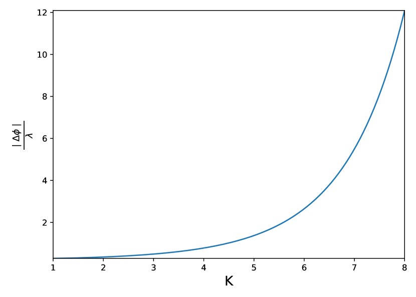
Figure 1: For slow-roll thawing quintessence, the field excursion $|\Delta\phi|$ divided by $\lambda\equiv|V^{\prime}(\phi_{i})/V(\phi_{i})|$ as a function of $K\equiv\sqrt{1-4V^{\prime\prime}(\phi_{i})/3V(\phi_{i})}$, where $\phi_{i}$ is the initial value of $\phi$.

Now we will solve for $w_{0}$, the present-day value of $w$, as a function of $\lambda$ and $K$. From Ref. Chiba , we have

$$1+w(t)=\frac{3}{4}\Biggr{(}\frac{V^{\prime}(\phi_{i})}{kt_{\Lambda}V^{\prime\prime}(\phi_{i})}\Biggr{)}^{2}\Biggr{(}\frac{kt_{\Lambda}\cosh(kt)\sinh({t}/{t_{\Lambda}})-\sinh(kt)\cosh({t}/{t_{\Lambda}})}{\sinh[2]({t}/{t_{\Lambda}})}\Biggr{)}^{2}$$ (16)

Taking $t$ equal to the present-day time from Eq. (13), we obtain

$$1+w_{0}=\frac{\lambda^{2}}{3K^{2}(1-K^{2})^{2}}\frac{(1-\Omega_{\phi 0})^{1-K}}{\Omega_{\phi 0}}\Biggr{[}(K-\Omega_{\phi 0}^{-\frac{1}{2}})(1+\sqrt{\Omega_{\phi 0}})^{K}+(K+\Omega_{\phi 0}^{-\frac{1}{2}})(1-\sqrt{\Omega_{\phi 0}})^{K}\Biggr{]}^{2}.$$ (17)

This result is illustrated in Fig. 2.

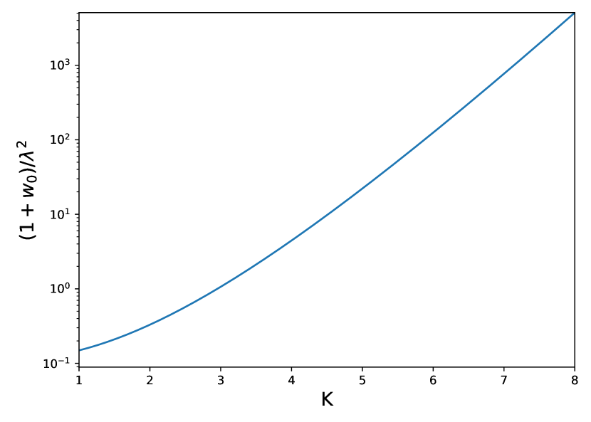
Figure 2: For slow-roll thawing quintessence, the present day value of the equation of state parameter, $1+w_{0}$, divided by $\lambda\equiv|V^{\prime}(\phi_{i})/V(\phi_{i})|$ as a function of $K\equiv\sqrt{1-4V^{\prime\prime}(\phi_{i})/3V(\phi_{i})}$, where $\phi_{i}$ is the initial value of $\phi$.

In the limit where $K\rightarrow 1$ ($V^{\prime\prime}\rightarrow 0$), we obtain the corresponding expression for $(1+w_{0})/\lambda^{2}$ for a linear potential ScherrerSen .

Finally, we can combine Eqs. (15) and (17) to eliminate $\lambda$, giving

$$1+w_{0}=\frac{3}{4}\Delta\phi^{2}\Biggr{[}\frac{(K-\Omega_{\phi 0}^{-\frac{1}{2}})(1+\sqrt{\Omega_{\phi 0}})^{K}+(K+\Omega_{\phi 0}^{-\frac{1}{2}})(1-\sqrt{\Omega_{\phi 0}})^{K}}{(1+\sqrt{\Omega_{\phi 0}})^{K}-(1-\sqrt{\Omega_{\phi 0}})^{K}-2K\sqrt{\frac{\Omega_{\phi 0}}{1-\Omega_{\phi 0}}}(1-\Omega_{\phi 0})^{\frac{K}{2}}}\Biggr{]}^{2}.$$ (18)

This result is illustrated in Fig. (3) .

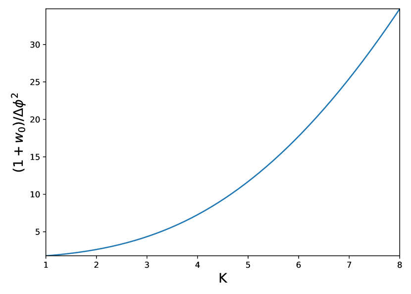
Figure 3: For slow-roll thawing quintessence, the present day value of the equation of state parameter, $1+w_{0}$, divided by the square of the field excursion, $\Delta\phi$, as a function of $K\equiv\sqrt{1-4V^{\prime\prime}(\phi_{i})/3V(\phi_{i})}$, where $\phi_{i}$ is the initial value of $\phi$.

Now consider the constraints that the refined Swampland conjecture (in the form of Eq. 8) places on these slow-roll thawing models when combined with observational constraints. Observational limits on slow-roll thawing models have been considered by Chiba, et. al. CDT , Smer-Berreto and Liddle SL , and Durrive, et al. durrive2018 . Of these papers, the treatment in Refs. CDT and durrive2018 is most similar to the discussion here. Both of these papers use the methodology of Refs. ds1 ; Chiba ; ds2 , along with observational data, to provide constraints in the $K,w_{0}$ plane. Ref. SL takes a somewhat different approach, deriving observational constraints on the Pseudo-Nambu-Goldstone Boson (PNGB) potential

$$V(\phi)=M^{4}\left[1+\cos(\phi/f)\right],$$ (19)

and then converting those constraints into limits on $K$ and $w_{0}$. Here we will use the limits derived in Ref. durrive2018 , but we will return to the approach in Ref. SL at the end of the paper.

Ref. durrive2018 derives limits on the slow-roll thawing models using the Planck 2015 release Planck , type Ia supernova observations from SDSS-II and SNLS Betoule , and baryon acoustic oscillation (BAO) measurements BAO1 ; BAO2 ; BAO3 . The resulting $2\sigma$ confidence limits in the plane defined by $w_{0}$ and $K$ can be mapped directly onto the models examined here. Using Eq. (18), we can transform these limits into a corresponding region in the plane defined by $|\Delta\phi|$ and $K$; this region is presented in Fig. 4. (Note that we fix $\Omega_{\phi 0}=0.69$, while Durrive et al. marginalize over this quantity. However, their corresponding distribution for $\Omega_{\phi 0}$ (marginalized over $w_{0}$) is strongly peaked near our value, and Eqs. (15), (17), and (18) are slowly-varying functions of $\Omega_{\phi 0}$, so our results are relatively insensitive to the assumed value for $\Omega_{\phi 0}$).

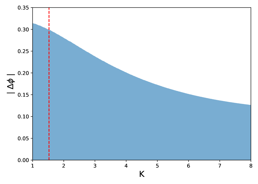
Figure 4: Observational constraints on slow-roll thawing quintessence from Ref. durrive2018 mapped onto the $|\Delta\phi|$, $K$ plane using the results of the present paper, where $\Delta\phi$ is the distance traversed by the field up to the present, and $K\equiv\sqrt{1-4V^{\prime\prime}(\phi_{i})/3V(\phi_{i})}$, with $\phi_{i}$ the initial value of $\phi$. The area outside of the shaded blue region corresponds to the $2\sigma$ excluded region in Ref. durrive2018 . The region to the right of the vertical red line satisfies the refined de Sitter conjecture with $c>1$.

If we use the limit $-V^{\prime\prime}/V>1$ for the refined de Sitter conjecture, then the region allowed by this conjecture lies to the right of the vertical red dashed line: namely, $K>\sqrt{7/3}=1.53$. From Fig. 4, it is clear that for the entire region satisfying both the observational constraints and the refined de Sitter conjecture, we have $|\Delta\phi|<0.3$. Thus, for slow-roll thawing quintessence models consistent with current observations, the distance conjecture becomes redundant; it is satisfied whenever the refined de Sitter conjecture is satisfied, while the converse is not true.

In the same way we can use Eq. (17) to transform the observational limits from Ref. durrive2018 into a corresponding region in the plane defined by $\lambda$ and $K$; this region is presented in Fig. 5.

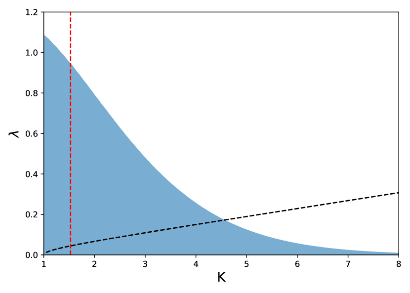
Figure 5: Observational constraints on slow-roll thawing quintessence from Ref. durrive2018 mapped onto the $\lambda$, $K$ plane using the results of the present paper, where $\lambda\equiv|V^{\prime}(\phi_{i})/V(\phi_{i})|$ and $K\equiv\sqrt{1-4V^{\prime\prime}(\phi_{i})/3V(\phi_{i})}$, with $\phi_{i}$ the initial value of $\phi$. The area outside of the shaded blue region corresponds to the $2\sigma$ excluded region in Ref. durrive2018 . The region to the right of the vertical red line satisfies the refined de Sitter conjecture with $-V^{\prime\prime}/V>1$. The region below the black curve was excluded from consideration in Ref. Raveri (see text).

As expected, one can find initial conditions consistent with observations for arbitrarily large values of $K$; however, as the curvature becomes larger, the value of $\lambda$ must become increasingly finely tuned to smaller values. This corresponds to placing the field initially closer to a local maximum in the potential. Obviously, these finely-tuned initial conditions are less plausible, but the question of what actually defines fine-tuning is, to some extent, arbitrary. However, we can take advantage of the form of the allowed region to make some plausible statements about fine tuning. For the region

$$\sqrt{7/3}<K<5,$$ (20)

the corresponding value of $\lambda$ is $\sim 0.1-1$, which would certainly not be considered fine tuned. On the other hand, for $K>6$, we have $\lambda<0.05$, with $\lambda$ approaching zero very rapidly as $K$ increases beyond this value. Hence, a plausible region consistent with observations, allowed by the refined de Sitter conjecture, and not particularly fine tuned is defined by Eq. (20).

This conclusion differs somewhat from that in Raveri et al. Raveri , who found a strong tension between the refined de Sitter conjecture and potentials of the form given by Eq. (9). However, these two results are not inconsistent. First note that Ref. Raveri used the cutoff $c\phi_{i}<0.0447$, which eliminates the smallest values of $\lambda$. This cutoff corresponds to the region below the black curve in Fig. 5. We have discounted some of this region already as corresponding to fine-tuned values of $\lambda$, but this does not account for our large allowed region with $K<5$. This region is downweighted in Ref. Raveri because these authors use a flat prior on the quantity $B/\rho_{\phi 0}$, which disfavors larger values of $c$ (corresponding to larger $K$ in our discussion.) A similar effect can be seen in comparing the observational constraints (without Swampland considerations) in Refs. CDT and durrive2018 to those in Ref. SL . Both CDT and durrive2018 find broad observationally-allowed regions in the $1+w_{0}$, $K$ plane. Ref. SL , on the other hand, adopts an approach similar to that of Raveri et al., beginning with a PNGB potential (Eq. 19) and deriving a corresponding excluded region for $K$ and $w_{0}$. The prior on $K$ in this case is highly non-uniform, resulting in a much smaller allowed region. Indeed, if we were to use the observational constraints of Ref. SL and repeat our analysis here, our conclusions would be much closer to those of Ref. Raveri . Neither approach is intrinsically more correct; the difference simply illustrates that the constraints on quintessence models are very sensitive to the assumed priors.

The results presented here by no means exhaust the various Swampland conjectures that have been proposed. For example, Bedroya and Vafa BV have recently proposed the “trans-Planckian censorship conjecture,” with the corresponding cosmological consequences examined in Ref. HBBR . However, the formalism we have utilized here for slow-roll thawing quintessence is particularly well suited to examining the refined de Sitter conjecture in the form of Eq. (8), as this formalism naturally accounts for the behavior of scalar fields near the maximum of potentials with negative curvature.

References

- (1) M. Kowalski et al., Astrophys. J. 686, 749 (2008).
- (2) M. Hicken et al., Astrophys. J. 700, 1097 (2009).
- (3) R. Amanullah et al., Astrophys. J. 716, 712 (2010).
- (4) N. Suzuki et al., Astrophys. J. 746, 85 (2012).
- (5) G. Hinshaw, et al., Astrophys. J. Suppl. 208, 19 (2013).
- (6) P.A.R. Ade, et al., Astron. Astrophys. 571, A16 (2014).
- (7) M. Betoule et al., Astron. Astrophys. 568, A22 (2014).
- (8) B. Ratra and P.J.E. Peebles, Phys. Rev. D 37, 3406 (1988).
- (9) C. Wetterich, Astron. Astrophys. 301, 321 (1995).
- (10) P.G. Ferreira and M. Joyce, Phys. Rev. Lett. 79, 4740 (1997).
- (11) E.J. Copeland, A.R. Liddle, and D. Wands, Phys. Rev. D57, 4686 (1998).
- (12) R.R. Caldwell, R. Dave and P. J. Steinhardt, Phys. Rev. Lett. 80, 1582 (1998).
- (13) A.R. Liddle and R.J. Scherrer, Phys. Rev. D 59, 023509 (1999).
- (14) P.J. Steinhardt, L.M. Wang and I. Zlatev, Phys. Rev. D 59, 123504 (1999).
- (15) E.J. Copeland, M. Sami, and S. Tsujikawa, Int. J. Mod. Phys. D 15, 1753 (2006).
- (16) N. Arkani-Hamed, L. Motl, A. Nicolis, and C. Vafa, JHEP 06, 060 (2007).
- (17) H. Ooguri and C. Vafa, Nucl. Phys. B 766, 21 (2007).
- (18) M. Scalisi and I. Valenzuela, JHEP 08, 160 (2019).
- (19) G. Obied, H. Ooguri, L. Spodyneiko, and C. Vafa, arXiv:1806.08362.
- (20) L. Heisenberg, J. Bartelmann, R. Brandenberger, and A. Refregier, Phys. Rev. D98, 123502 (2018).
- (21) P. Agrawal, G. Obied, P.J. Steinhardt, and C. Vafa, Phys. Lett. B 784, 271 (2018).
- (22) Y. Akrami, R. Kallosh, A. Linde, and V. Vardanyan, Fortschr. Phys. 67, 1800075 (2019).
- (23) M. Raveri, W. Hu, and S. Sethi, Phys. Rev. D99, 083518 (2019).
- (24) S.K. Garg and C. Krishnan, JHEP 11 075 (2019).
- (25) R.J. Scherrer, Phys. Lett. B 798, 134981 (2019).
- (26) G. Montefalcone, P.J. Steinhardt, and D.H. Wesley, JHEP 06, 091 (2020).
- (27) E.O. Colgain and H. Yavartanoo, arXiv:1905.02555.
- (28) A. Banerjee, et al., arXiv:2006.00244.
- (29) M. Cicoli, G. Dibitetto, and F.G. Pedro, arXiv:2007.11011.
- (30) S. Brahma and Md. Wali Hossain, JHEP 06, 070 (2019).
- (31) A.R. Solomon and M. Trodden, arXiv:2004.09526.
- (32) S. Brahma and Md. Wali Hossain, arXiv:2007.06425.
- (33) H. Geng, Phys. Lett. B 805, 135430 (2020).
- (34) H. Ooguri, E. Palti, G. Shiu, and C. Vafa, Phys. Lett. B 788, 180 (2019).
- (35) R.R. Caldwell and E.V. Linder, Phys. Rev. Lett. 95, 141301 (2005).
- (36) S. Dutta and R. J. Scherrer, Phys. Rev. D78, 123525 (2008).
- (37) T. Chiba, Phys. Rev. D79, 083517 (2009).
- (38) S. Dutta, E. N. Saridakis and R. J. Scherrer, Phys. Rev. D79, 103005 (2009).
- (39) P. Agrawal and G. Obied, JHEP 6, 103 (2019).
- (40) R.J. Scherrer and A.A. Sen, Phys. Rev. Dbf 77, 083515 (2008).
- (41) T. Chiba, A. De Felice, and S. Tsujikawa, Phys. Rev. D87, 083505 (2013).
- (42) V. Smer-Barreto and A.R. Liddle, JCAP 1, 023 (2017).
- (43) J.-B. Durrive, J. Ooba, K. Ichiki, and N. Sugiyama, Phys. Rev. D 97, 043503 (2018).
- (44) P.A.R. Ade, et al., Astron. Astrophys. 594, A13 (2016).
- (45) F. Beutler, et al., Mon. Not. R. Astron. Soc. 416, 3017 (2011).
- (46) L. Anderson, et al. Mon. Not. R. Astron. Soc. 441, 24 (2014).
- (47) A.J. Ross, et al., Mon. Not. R. Astron. Soc. 449, 835 (2015).
- (48) A. Bedroya and C. Vafa, arXiv:1909.11063.
- (49) L. Heisenberg, M. Bartelmann, R. Brandenberger, and A. Refregier, arXiv:2003.13283.