Construction and Extension of Dispersion Models

Abstract

There are two main classes of dispersion models studied in the literature: proper (PDM), and exponential dispersion models (EDM). Dispersion models that are neither proper nor exponential dispersion models are termed here non-standard dispersion models. This paper exposes a technique for constructing new proper dispersion models and non-standard dispersion models. This construction provides a solution to an open question in the theory of dispersion models about the extension of non-standard dispersion models.

Given a unit deviance function, a dispersion model is usually constructed by calculating a normalising function that makes the density function integrates one. This calculation involves the solution of non-trivial integral equations. The main idea explored here is to use characteristic functions of real non-lattice symmetric probability measures to construct a family of unit deviances that are sufficiently regular to make the associated integral equations tractable. It turns that the integral equations associated to those unit deviances admit a trivial solution, in the sense that the normalising function is a constant function independent of the observed values. However, we show, using the machinery of distributions (i.e., generalised functions) and expansions of the normalising function with respect to specially constructed Riez systems, that those integral equations also admit infinitely many non-trivial solutions. On the one hand, the dispersion models constructed with constant normalising functions (corresponding to the trivial solution of the integral equation) are all proper dispersion models; on the other hand, the normalising functions arising from non-trivial solutions of the integral equation generate dispersion models that are non-standard models. As a consequence, the cardinality of the class of non-standard dispersion models is larger than the cardinality of the class of real non-lattice symmetric probability measures.

Key-words: Dispersion models, Exponential dispersion models, Proper dispersion models, Generalised functions.

1 Introduction

Dispersion models (DMs) are parametric families of probability measures defined on Euclidean spaces, which play an essential rule in statistics (Jørgensen, 1987a, 1997). Several classic families of probability measures such as the normal, Poisson, binomial, gamma. inverse-gaussian, von Mises, gamma-Poisson compound, and simplex families are DMs. The mathematical properties common to all DMs allow constructing a sound and well-elaborated theoretical machinery to perform statistical inference for those parametric families (Jørgensen, 1987a, 1997; Cordeiro et al., 2019). DMs naturally appear in many statistical applications since they form the basis of several major classes of statistical models as generalized linear models (McCullagh et al., 1989; Jørgensen, 1987a, b), generalized additive models, and variants of state-space models (Jørgensen et al., 1996a; Fahmeir et al., 2001). In this paper, we introduce some techniques for constructing new DMs which allow us to set a lower bound to the cardinality of some important classes of DMs; we will show that those classes of DMs are indeed vast.

There are two major classes of DMs studied in detail in the literature: exponential dispersion models (EDMs) and proper dispersion models (PDMs). Dispersion models that are neither a PDM nor an EDM are termed here non-standard dispersion models (NSDMs). These models (sic.) ”are still not well understood, mainly for lack of examples of this kind” and because methods for generating those models are currently non-existent (Jørgensen, 1997, p. 8, last paragraph). In this paper, we study a relatively general method for constructing NSDMs. We show that the cardinality of the class of NSDMs is, in fact, large, at least as large of the cardinality of non-lattice real distributions that are symmetric about zero. Some of the ideas exposed in full details here were sketched in Cordeiro et al. (2019), although the construction presented here takes advantage of mathematical tools that are even not mentioned there (e.g., the construction of a special representation based on the theory of Riez systems).

The paper is organized as follows. Section 2 presents a short review on dispersion models and sets the basic notation. Section 3 discusses the general problem of construction of DMs when a unit deviance is given while section 3.1 discuss some details of the generation of PDMs, section 3.2 presents a technique for generating PDMs based on characteristic functions that extends naturally to the problem of generating NSDMs in section 3.3. Section 4 presents some discussion and examples. Appendix A presents the proof of three technical lemmas and some required basic results on the theory of Riez systems (a generalisation of the notion of basis).

2 A Short Review on One-Dimensional Dispersion Models

Consider a parametric family of probability measures $\mathcal{P}=\left\{P_{\mu\lambda}:\mu\in\Omega,\lambda\in\Lambda\right\}$ defined on $(\mathbb{R},\mathcal{B}(\mathbb{R}))$, where the parametrisation given by $(\mu,\lambda)$ is identifiable (i.e., the mapping $(\mu,\lambda)\mapsto P_{\mu\lambda}$ is a bijection between $\Omega\times\Lambda$ and $\mathcal{P}$). Assume that $\mathcal{P}$ is dominated by a $\sigma$-finite measure $\upsilon$ with support $\mathcal{Y}\subseteq\mathbb{R}$, $\Omega\subseteq\mathcal{Y}$ is open, $\Lambda\subseteq\mathbb{R}_{+}$ is an interval bounded from the left and unbounded to the right, and that for each $(\mu,\lambda)\in\Omega\times\Lambda$ a version of the Radon-Nykodyn derivative of $P_{\mu\lambda}$ with respect to $\upsilon$ is of the form

$$\frac{dP_{\mu\lambda}}{d\upsilon}(y)\mathrel{\overset{\makebox[0.0pt]{\mbox{\tiny def}}}{=}}p(y;\mu,\lambda)=a(y;\lambda)\exp\left\{-\lambda\,d(y;\mu)\right\},\mbox{ for all }y\in\mathcal{Y}.$$ (1)

Here $a:\mathcal{Y}\times\Lambda\rightarrow\mathbb{R}_{+}$ and $d:\mathcal{Y}\times\Omega\rightarrow\mathbb{R}_{+}$ are given suitable functions. If the function $d$ is such that $d(\mu;\mu)=0$ for all $\mu\in\Omega$ and $d(y;\mu)>0$ for all $(y,\mu)\in\mathcal{Y}\times\Omega$ such that $y\neq\mu$, then $d$ is said to be a unit deviance and the family $\mathcal{P}$ is the dispersion model (DM) generated by the unit deviance $d$. The parameters $\mu$ and $\lambda$ are called the position parameter and the index parameter, respectively, $\Lambda$ is the index set, and $a$ is termed the normalizing function. Without loss of generality we assume that $\Lambda=\mathbb{R}_{+}$.

A dispersion model with density (1) is said to be a proper dispersion model generated by a unit deviance $d$ when the normalizing function $a$ factorizes as,

$$a(y;\lambda)=a_{0}(\lambda)\,b(y),\mbox{ for all }(y,\lambda)\in\mathcal{Y}\times\Lambda\,,$$

where $a_{0}:\Lambda\rightarrow\mathbb{R}_{+}$ and $b:\mathcal{Y}\rightarrow\mathbb{R}_{+}$ are suitable functions. A dispersion model generated by a unit deviance $d$ is said to be an exponential dispersion model when the unit deviance takes the form

$$d(y;\mu)=yf(\mu)+g(\mu)+h(y)\,,\mbox{ for all }y\in\mathcal{Y}\mbox{ and }\mu\in\Omega\,,$$ (2)

for suitable functions $f,g$ and $h$. Examples of PDMs are the von Mises, the simplex, the normal, the gamma and the inverse Gaussian families of distributions. The normal, gamma, inverse Gaussian, Poisson and gamma compound Poisson families of distributions are classic examples of EDMs. There are only three PDMs that are also EDMs: the normal, the gamma and the inverse Gaussian families of distributions (Jørgensen, 1997, Theorem 5.6.).

3 The Problem of Construction of Dispersion
Models

We shall be concerned below with the general problem of constructing DMs in a process that will enable us to access the extension of this class of parametric families. Not all unit deviances generate a DM. Indeed, a unit deviance $d$ generates a DM if, and only if, it is possible to find a normalising function $a:\mathcal{Y}\times\Lambda\rightarrow\mathbb{R}_{+}$ such that the integral of the density given by (1) integrates $1$, i.e., the function $a$ is the solution of the integral equation

$$\int_{\mathcal{Y}}a(y;\lambda)\exp\left\{-\lambda d(y;\mu)\right\}\upsilon(dy)=1,\mbox{ for all }(\mu,\lambda)\in\Omega\times\Lambda\,.$$ (3)

Note that the solution $a$ should be a function independent of the position parameter $\mu$. Posed in this generality, this problem is hard to solve since it is difficult to establish even whether the integral equation (3) has a solution. However, we will present a technique for constructing many examples where the problem of generating dispersion models tractable.

3.1 Generation of Proper Dispersion Models

We turn now to the problem of generating proper dispersion models from a given unit deviance $d$. In that case, the normalising function factorises as $a(y;\lambda)=a_{0}(\lambda)\,b(y)$, for all $(y,\lambda)\in\mathcal{Y}\times\Lambda$. Since $p(\,\cdot\,;\mu,\lambda)$ is a probability density and $\exp\left\{-\lambda d(\,\cdot\,;\mu)\right\}$ take only positive values, then the function $a=a_{0}\,.b$ takes only positive values in the support of $\upsilon$. We assume then, without loss of generality, that both $a_{0}$ and $b$ take only positive values. When working with PDMs the integral equation (3) takes the form

$$a_{0}(\lambda)\int_{\mathcal{Y}}b(y)\exp\left\{-\lambda d(y;\mu)\right\}\upsilon(dy)=1,\mbox{ for all }(\mu,\lambda)\in\Omega\times\Lambda\,.$$ (4)

Any function $b:\mathcal{Y}\longrightarrow\mathbb{R}_{+}$ such that the integral $\int_{\mathcal{Y}}b(y)\exp\left\{-\lambda d(y;\mu)\right\}\upsilon(dy)$ is finite and does not depend on the position parameter $\mu$ generates a proper dispersion model. In the case such a function $b$ exists, defining

$$a_{0}(\lambda)=\frac{1}{\int_{\mathcal{Y}}b(y)\exp\left\{-\lambda d(y;\mu)\right\}\upsilon(dy)}\,,\,\,\mbox{ for each $\lambda\in\Lambda$,}$$

yields a solution for equation (4) and the densities of the form given by (1) defined with $a_{0}$ and $b$ correspond to the densities of a proper dispersion model. Note that $\int_{\mathcal{Y}}b(y)\exp\left\{-\lambda d(y;\mu)\right\}\upsilon(dy)>0$ since both $b$ and $\exp\left\{-\lambda d(\,\cdot\,;\mu)\right\}$ take only positive values in the support of $\upsilon$. In particular, any function $b\in L^{1}_{\upsilon}(\mathbb{R})$ such that $\int_{\mathcal{Y}}b(y)\exp\left\{-\lambda d(y;\mu)\right\}\upsilon(dy)$ does not depend on $\mu$ can be used to construct a PDM. We present next a technique for obtaining solutions of the equation (4) for a rich class of unit deviances.

3.2 Generation of Dispersion Models via Unit Deviances Constructed with Characteristic Functions

We will use below the fact that a unit deviance is a non-negative definite function and therefore, according to the Bochner’s theorem, it is the Fourier transform of a certain probability measure. This fact form the basis of the following proposition.

Proposition 1.

Suppose that the function $d:\mathbb{R}\times\Omega\rightarrow\mathbb{R}_{+}$ is of the form

$$d(y;\mu)=\left\{1-\varphi(y-\mu)\right\}|\phi(y-\mu)|,\mbox{ for all }(y,\mu)\in\mathbb{R}\times\Omega\,,$$ (5)

where $\varphi$ and $\phi$ are characteristic functions of real absolute continuous probability measures that are symmetric around zero and are not lattice distributions. Then the function $d$ is a unit deviance and there exists a PDM in $(\mathbb{R},\mathcal{B}(\mathbb{R}))$ dominated by the Lebesgue measure generated by the unit deviance $d$. Moreover, the function $b$ defining the PDM above is constant.

Recall that a real distribution concentrated on a set of the form $\{a+nh,n=0,\pm 1,\pm 2,\dots\}$ for some $a,h\in\mathbb{R}$ and $h>0$ is called a lattice distribution.

A consequence of the proposition above is that the cardinality of the class of PDMs is larger than the square of the cardinality of the class of all the characteristic functions of real absolute continuous probability measures that are symmetric around zero and are not lattice distributions. Proof: $d$ is a unit deviance: The functions $\varphi$ and $\phi$ take only real values because they are characteristic functions of distributions that are symmetric about zero. Moreover, $\varphi(0)=\phi(0)=1$ and $|\varphi(t)|\leq 1$ and $|\phi(t)|\leq 1$ for all $t\in\mathbb{R}$ since $\varphi$ and $\phi$ are characteristic functions (Lucaks, 1970) and, $|\varphi(t)|<1$ and $|\phi(t)|<1$ for all $t\in\mathbb{R}\setminus\{0\}$ because they are characteristic functions of non lattice distributions (Ushakov, 1999, Theorem 1.1.3, p.2). Therefore, the function $d$ defined in (5) is a unit deviance, which is referred as the unit deviance generated by the characteristic functions $\varphi$ and $\phi$.

Obtaining a weak solution of the integral equation (4): Take a fixed and arbitrary $\lambda_{0}\in\mathbb{R}_{+}$. In the context of this proposition, equation (3) becomes, for all $\mu\in\mathbb{R}$,

$$1 = \int_{\mathbb{R}}a(y,\lambda_{0})\exp\left\{-\lambda_{0}[1-\varphi(y-\mu)]|\phi(y-\mu)|\right\}dy$$

(since $$\varphi \phi$$ and are characteristic functions taking values

in $$\mathbb{R}$$ and therefore are symmetric about zero)

$$= \int_{\mathbb{R}}a(y,\lambda_{0})\exp\left\{-\lambda_{0}[1-\varphi(\mu-y)]|\phi(\mu-y)|\right\}dy=\int_{\mathbb{R}}a_{\lambda_{0}}(y)K_{\lambda_{0}}(\mu-y)dy\,.$$

Here, $K_{\lambda}:\mathcal{Y}\rightarrow(0,1]$ is a kernel given by $K_{\lambda}(y)=\exp\left\{-\lambda[1-\varphi(y)]|\phi(y)|\right\}$, for all $y\in\mathcal{Y}$ and $\lambda\in\Lambda$. Note that , for each $\lambda\in\Lambda$, $0<K_{\lambda}(y)\leq 1$, for all $y\in\mathcal{Y}$.

We want to solve the integral equation above for $a_{\lambda_{0}}(\,\cdot\,)=a(\,\cdot\,,\lambda_{0})$ using the kernel $K_{\lambda_{0}}(\,\cdot\,)$. Assume that $a_{\lambda_{0}}$ is in the Schwartz class, that is, $a_{\lambda_{0}}\in\mathcal{S}(\mathbb{R})\mathrel{\overset{\makebox[0.0pt]{\mbox{\tiny def}}}{=}}\left\{f:\mathbb{R}\rightarrow\mathbb{R}\in C^{\infty}:\forall\alpha,\beta\in\mathbb{N},\sup_{x\in\mathbb{R}}\left|f^{(n)}(x)x^{\alpha}\right|<\infty\right\}$. Equation (3.2) simplifies to the following convolution equation,

$$\left(a_{\lambda_{0}}*K_{\lambda_{0}}\right)(\mu)=1\,\mbox{, for all }\mu\in\mathbb{R}\,.$$ (7)

Here, the convolution operator $"*"$ refers to the convolution between functions. Since the function $a_{\lambda_{0}}\in\mathcal{S}(\mathbb{R})$ and $K_{\lambda}$ is continuous and bounded, then $a_{\lambda_{0}}*K_{\lambda_{0}}$, $\mathcal{F}\left(a_{\lambda_{0}}\right)$, $\mathcal{F}\left(K_{\lambda_{0}}\right)$ and $\mathcal{F}\left(a_{\lambda_{0}}*K_{\lambda_{0}}\right)$ are all well defined. Here, $\mathcal{F}\left(f\right)$ denotes the Fourier transform of the function $f$ and $\mathcal{F}^{-1}$ denotes the inverse Fourier transform. Therefore, the convolution equation (7) is equivalent, in the sense of distributions, to

$$\mathcal{F}\left[a_{\lambda_{0}}*K_{\lambda_{0}}\right](\mu)=\mathcal{F}\left[a_{\lambda_{0}}\right](\mu)\,.\,\mathcal{F}\left[K_{\lambda_{0}}\right](\mu)=\mathcal{F}[f](\omega)=\delta(\mu)\,,$$ (8)

where the function $f:\mathbb{R}\rightarrow\mathbb{R}$ is the constant function equal to $1$ (i.e., $f(t)=1$, for all $t\in\mathbb{R}$) and $\delta$ is the Dirac distribution. Since integration of the Dirac distribution times a test function corresponds to evaluating the test function at zero, we have that, for each $\lambda_{0}\in\Lambda$,

$$a(y;\lambda_{0})\mathrel{\overset{\makebox[0.0pt]{\mbox{\tiny def}}}{=}}a_{\lambda_{0}}(y) = \mathcal{F}^{-1}_{y}\left\{\frac{\delta(\mu)}{\mathcal{F}\left[K_{\lambda_{0}}\right](\mu)}\right\}=\int_{-\infty}^{\infty}\frac{1}{2\pi}e^{iy\mu}\frac{\delta(\mu)}{\mathcal{F}\left[K_{\lambda_{0}}\right](\mu)}d\mu$$

$$= \frac{1}{2\pi}\frac{1}{\mathcal{F}\left[K_{\lambda_{0}}\right](0)}$$

$$= \frac{1}{2\pi}\frac{1}{\int_{-\infty}^{\infty}e^{0i}\exp\left\{-\lambda_{0}[1-\varphi(y-\mu)]|\phi(\mu-y)|\right\}dy}$$

$$= \frac{1}{2\pi}\frac{1}{\int_{-\infty}^{\infty}\exp\left\{-\lambda_{0}[1-\varphi(z)]|\phi(z)|\right\}dz}\mathrel{\overset{\makebox[0.0pt]{\mbox{\tiny def}}}{=}}a_{0}(\lambda_{0})\,,$$

where the function $a_{0}$ does not depend neither on $\mu$ nor on $y$. Therefore, the DM generated by $d$ is a PDM with the function $a_{0}(\lambda)=\alpha_{\lambda}$ and $b(y)=1$, $\forall y\in\mathbb{R}$. $\sqcup\!\!\!\!\sqcap$

Corollary 2.

The unit deviance $d$ defined by (5) does not generate an EDM and cannot be expressed in the form given by (2).

Proof: The only PDMs that are also EDMs are the normal, the gamma and the inverse Gaussian families of distributions (Jørgensen, 1997, Theorem 5.6.). Direct verification shows that the unit deviance of the normal, the gamma and the inverse Gaussian families cannot be expressed as (5). $\sqcup\!\!\!\!\sqcap$

3.3 Construction of Non-Standard Dispersion Models

We say that the solution the integral equation (3.2) of the form $a(y;\lambda)=a_{0}(\lambda)$ is a trivial solution because it does not depend on the observed values $y$. As discussed above, the integral equations (3.2) associated with unit deviances of the form (8) have a trivial solution, which generate PDMs. We show below that those trivial solutions can be used as a basis for obtaining infinitely many non trivial solutions that correspond to NSDMs. In this section we assume that $\mathcal{Y}=\mathbb{R}$ and $\Lambda=\mathbb{R}_{+}$. Moreover, when not explicitly mentioned $\lambda$ will be an arbitrary element of $\Lambda$.

The idea explored here is that, for any $\lambda\in\Lambda$, the constant function $a_{0}:\mathbb{R}_{+}\rightarrow\mathbb{R}_{+}$, given by $a_{0}(\lambda)=1/\int_{\mathbb{R}}K_{\lambda}(y)dy\mathrel{\overset{\makebox[0.0pt]{\mbox{\tiny def}}}{=}}\tilde{a}_{\lambda}$ is a trivial solution of

$$1=\{a_{\lambda}*K_{\lambda}\}(\mu)=\int_{\mathbb{R}}a_{\lambda}(y)K(\mu-y)dy=\tilde{a}_{\lambda}\,\langle 1,K(\,\cdot\,-\mu)\rangle_{L^{2}(\mathbb{R})}\,,$$ (10)

which does not depend on the position parameter $\mu$. Taking this trivial solution as a starting point we obtain new solutions by adding a function orthogonal to each $K(\,\cdot\,-\mu)$ (for all $\mu\in\mathbb{R}$). This new function will solve also the equation (10) above. Consider the subspace of $L^{2}(\mathbb{R})$ given by

$$V=cl_{L^{2}(\mathbb{R})}\left\{span\left[K_{\lambda}(\,\cdot\,-\mu)\right]\right\}\subseteq L^{2}(\mathbb{R})\,,$$

We show in Lemma 3 (in the appendix A) that

$$P^{0}\mathrel{\overset{\makebox[0.0pt]{\mbox{\tiny def}}}{=}}\left\{f:\mathbb{R}\rightarrow\mathbb{R}_{+}\mbox{ in }L^{2}(\mathbb{R}):f\mbox{ is symmetric about }0,\right\}\subseteq V^{\perp}.$$

Therefore, $V^{\perp}$ is not empty. Consider now a function $g_{\lambda}:\mathbb{R}\longrightarrow\mathbb{R}$ given by $g_{\lambda}(y)=\tilde{a}_{\lambda}+f(y)$, $\forall y\in\mathbb{R}$ were $f:\mathbb{R}\longrightarrow\mathbb{R}$ is in $V^{\perp}$ (e.g., $f\in P^{0}$). We have then

$$\langle g_{\lambda}(\,\cdot\,),K_{\lambda}(\,\cdot\,-\mu)\rangle_{L^{2}(\mathbb{R})} = \langle\tilde{a}_{\lambda}+f(\,\cdot\,),K_{\lambda}(\,\cdot\,-\mu)\rangle_{L^{2}(\mathbb{R})}$$

$$= \tilde{a}_{\lambda}\langle 1,K_{\lambda}(\,\cdot\,-\mu)\rangle_{L^{2}(\mathbb{R})}\,\,+\,\,\langle f(\,\cdot\,),K_{\lambda}(\,\cdot\,-\mu)\rangle_{L^{2}(\mathbb{R})}=1\,,$$

for each $\mu\in\mathbb{R}$. Therefore, $g_{\lambda}$ is a non-trivial solution of the integral equation associated to the unit deviance $d$ defined in (5).

Clearly, there are many non-trivial solutions to the integral equation (10), at least as many as the cardinality of $P^{0}$, which in particular includes all the probability density functions that are symmetric about zero which are in $L^{2}(\mathbb{R})$. The construction yielding the required characterisation of $V^{\perp}$ is given in appendix A.

4 Discussion and Examples

A unit deviance $d$ is said to be regular when $d$ is twice continuously differentiable in $\mathcal{Y}\times\Omega$ and $\partial^{2}d(y;\mu)/\partial\mu^{2}\geq 0$ for all $(y,\mu)\in\mathcal{Y}\times\Omega$. If $d$ is a regular unit deviance and $\mathcal{Y}=\Omega$, then the dispersion model generated by $d$ is said to be a regular dispersion model. Regularity plays a crucial rule in the theory of statistical inference for DMs (Jørgensen, 1997; Cordeiro et al., 2019) since it is required for establishing key asymptotic results (e.g., without regularity the observed Fisher information is not defined). Clearly, a unit deviance $d$ defined by a characteristic function as in (5) is regular if, and only if, the first two moments of the distributions with characteristic function $\varphi$ and $\phi$ are finite. To see that, note that the characteristic functions $\varphi$ and $\phi$ are twice continuous differentiable if, and only if, the first two central moments of the related probability measure are finite. It is easy to see that $\partial^{2}d(\mu;\mu)/\partial\mu^{2}>0$.

The technique described above allow us to construct many regular and non-regular unit deviances. For example, the unit deviance given by

$$d(y;\mu)=\left[1-\exp\left\{\left(y-\mu\right)^{2}/2\right\}\right]\left|\exp\left(y-\mu\right)^{2}/2\right|\,,$$

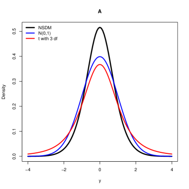
generated by the characteristic functions $\varphi$ and $\phi$ coinciding with the charactteristic function of the standard normal distribution is a regular PDM (see the panel A of Figure 1). Furthermore, the unit deviance

$$d(y;\mu)=\left\{1-\exp(|y-\mu|)\right\}|\exp(-t^{2}/2)|\,,$$

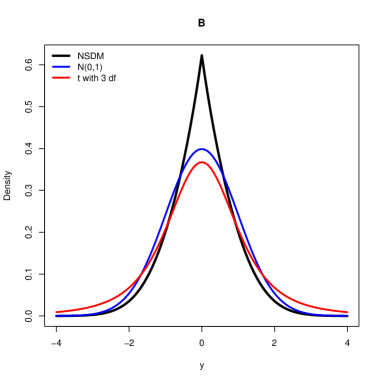
constructed with the characteristic function of the Cauchy and the normal distribution, is not a regular unit deviance (see the panel B of Figure 1). The characteristic functions of normal inverse Gaussian distributions (Barndorff-Nielsen, 1977) with vanishing asymmetry parameter generate regular unit deviances (since these distributions have finite moments of all orders). Note that the Cauchy distribution can be obtained as a limit of a sequence of symmetric normal inverse Gaussian distributions with increasing tail heaviness. The unit deviances generated by the characteristic functions of symmetric Lèvy-$\alpha$-stable distributions with the parameter $\alpha$ smaller than $2$ are other examples on non-regular unit deviances since the variances of those distributions are not finite, generating also non-regular NSDMs.

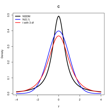
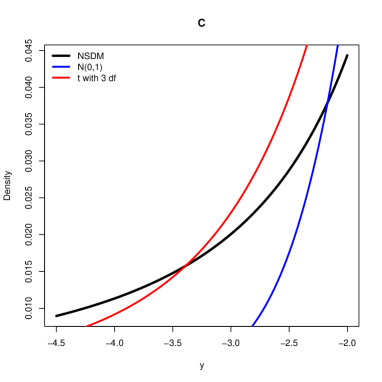
The panel C of Figure 2 depicts the density of the PDM generated by the characteristic functions $\varphi$ and $\phi$ coinciding with the characteristic function of the Laplace distribution, i.e.with the unit deviance

$$d(y;\mu)=\left\{1-\frac{1}{1+t^{2}}\right\}\left|\frac{1}{1+t^{2}}\right|.$$

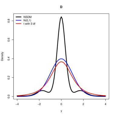
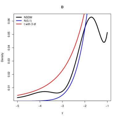
Note that this PDM is regular and has tails heavier than the $t$ distribution with $3$ degrees of freedom. Adding the $L^{2}(\mathbb{R})$ symmetric function $f(y)=\{\cos(y*3)+1\}\exp(-y^{2}/10)$ to the normalising function we obtain an example of a regular NSDM, see the panel D of Figure 2. We illustrated above the construction of a suite of unusual DMs.

Figure 1: Densities of NSDM (black), standard normal distribution (blue) and t distribution with $3$ degrees of freedom (red). In panel A the NSDM is generated by the characteristic functions of the standard normal distribution $\varphi(t)=\phi(t)=\exp(-t^{2}/2)$. In panel B the NSDM is generated by the characteristic functions of the Cauchy and the normal distribution, i.e., $\varphi(t)=\exp(-|t|)$ and $\phi(t)=\exp(-t^{2}/2)$.

Figure 2: Densities of NSDM (black), standard normal distribution (blue) and t distribution with $3$ degrees of freedom (red). In panel C the NSDM is generated by the characteristic functions of the Laplace distribution $\varphi(t)=\phi(t)=1/(1+t^{2})$. In panel D the NSDM is generated as in panel C but with a normalising function obtained by adding the $L^{2}(\mathbb{R})$ symmetric function $f(y)=\{\cos(y*3)+1\}\exp(-y^{2}/10)$ to the normalising function. Details of the left tail in the right panels.

Appendix A Three Technical Lemmas

Basic facts on Riez systems -

For convenience of the readers, we briefly expose some basic theory of Riez systems required for the proof of the three technical lemmas below. A complete exposition of the results on Riez systems below can be found in Krivoshein et al. (2016) from which we draw heavily in the next two paragraphs. Let $l^{2}$ be the Hilbert space of all the complex sequences $c=\{c_{n}\}_{n\in\mathbb{N}}=\{c_{n}\}$ such that the series $\sum_{n=1}^{\infty}|c_{n}|^{2}$ converges, endowed with the inner product $\langle c,d\rangle_{l^{2}}=\sum_{n=1}^{\infty}c_{n},\bar{d}_{n}$, defined for any $c=\{c_{n}\}\in l^{2}$ and $d=\{d_{n}\}\in l^{2}$, and the norm $||c||^{2}_{l^{2}}=\langle c,c\rangle_{l^{2}}$. A sequence $\left\{f_{n}\right\}_{n\in\mathbb{N}}=\left\{f_{n}\right\}$ in a given Hilbert space $H$ is said to be a Riez system (in $H$) with constants $A$ and $B$ ($A,B\in\mathbb{R}_{+}$) if for any sequence $c=\{c_{n}\}_{n\in\mathbb{N}}$ in $l^{2}$, the series $\sum_{n=1}^{\infty}c_{n}f_{n}$ converges in $H$ and

$$A\,\,||c||_{l^{2}}\leq\left|\left|\sum_{n=1}^{\infty}c_{n}f_{n}(\,\cdot\,)\right|\right|^{2}_{L^{2}(\mathbb{R})}\leq B\,\,||c||_{l^{2}}\,.$$

If the constants $A$ and $B$ are equal, the system is said to be tight.

If $\left\{f_{n}\right\}_{n\in\mathbb{N}}$ is a Riez system with constants $A$ and $B$, then it can be shown that $\left\{f_{n}:n\in\mathbb{N}\right\}$ is a basis of $V=cl_{H}\left[span\left\{f_{n},\,n\in\mathbb{N}\right\}\right]$ (Krivoshein et al., 2016, theorem 1.1.2), where $cl_{H}(A)$ is the closure of $A\subseteq H$ with respect to the topology of $H$. Moreover, if $\varphi$ is a function on $L^{2}(\mathbb{R})$ and $\{\varphi(\,\cdot\,+q):q\in\mathbb{Z}\}$ is a Riez system and a basis of a closed subspace $V$ of $L^{2}(\mathbb{R})$, then it can be proved that (Krivoshein et al., 2016, theorem 1.1.10) a function $f\in L^{2}(\mathbb{R})$ is orthogonal to $V$ if, and only if,

$$\sum_{q\in\mathbb{Z}}\widehat{f}(\xi+q)\overline{\widehat{\varphi}(\xi+q)}=0,\mbox{ for almost all }\xi\in\mathbb{R}\,\,.$$ (11)

Here $\widehat{f}$ is the Fourier transform of the function $f$ and $\overline{x}$ is the conjugate of the complex number $x$.

Preparation for the three lemmas

-

Consider the functional $K:\mathbb{R}\rightarrow(0,1]$ given by $K(y)=\exp\left\{-\lambda\left[1-\varphi(y)\right]|\phi(y)|\right\},\,\forall y\in\mathbb{R}$, where $\lambda>0$ (fixed), and the subspace $V\subseteq L^{2}(\mathbb{R})$ given by

$$V=cl_{L^{2}(\mathbb{R})}\left[span\left\{K(\,\cdot\,-\mu):\mu\in\mathbb{R}\right\}\right]\,.$$

Here $\varphi$ and $\phi$ are characteristic functions of a non-lattice distributions symmetric about zero. Moreover, $\phi$ is the characteristic function of an absolute continuous distribution, and therefore Clearly, $0<K(y)\leq 1$, $\forall y\in\mathbb{R}$, with equality if, and only if, $y=0$. Moreover, $K^{2}(y)\leq K(y)$, $\forall y\in\mathbb{R}$, and

$$||K(\,\cdot\,)||^{2}_{L^{2}(\mathbb{R})}=\int_{\mathbb{R}}\{K(y)\}^{2}dy\leq\int_{\mathbb{R}}K(y)dy\,.$$ (12)

Note that the function $\exp\left\{-\lambda\left[1-\varphi(\,\cdot\,)\right]\right\}$ is a characteristic function (see Ushakov, 1999, Corollary 1.3.4, p. 18). We show below that $K$ is also a characteristic function using the Bochner-Khintchine theorem (see Ushakov, 1999, Corollary 1.3.1, p. 8); i.e.we argue that $K(0)=1$ and that the function $K$ is non-negative definite. Clearly, $K(0)=\exp\left\{-\lambda\left[1-\varphi(0)\right]|\phi(0)|\right\}=1$. In order to prove that $K$ is non-negative definite, take an arbitrary $N\in\mathbb{N}$, $z_{1},\dots,z_{n}\in\mathbb{C}$, and $t_{1},\dots,t_{n}\in\mathbb{R}$. Then,

$$\sum_{j=1}^{N}\sum_{k=1}^{N}K(t_{j}-t_{k})z_{j}\bar{z}_{k} = \sum_{j=1}^{N}\sum_{k=1}^{N}\exp\left\{-\lambda\left[1-\varphi(t_{j}-t_{k})\right]|\phi(t_{j}-t_{k})|\right\}z_{j}\bar{z}_{k}$$

$$\geq \sum_{j=1}^{N}\sum_{k=1}^{N}\exp\left\{-\lambda\left[1-\varphi(t_{j}-t_{k})\right]\right\}z_{j}\bar{z}_{k}$$

$$\mbox{(since }\exp\left\{-\lambda\left[1-\varphi(\,\cdot\,)\right]\right\}\mbox{ is non-negative definite)}$$

$$\geq 0\,,$$

which implies that $K$ is non-negative definite, and therefore, $K$ is a characteristic function. As a consequence, $K$ is uniform continuous and, since $K$ takes only real values, the probability measure for which $K$ is the characteristic function is symmetric about zero.

Using substitution it is easy to see that for all $\mu\in\mathbb{R}$, (substituting, $y$ by $x-\mu$)

$$||K(\,\cdot\,-\mu)||^{2}_{L^{2}(\mathbb{R})}=\int_{\mathbb{R}}\{K(x-\mu)\}^{2}dx=\int_{\mathbb{R}}\{K(y)\}^{2}dy=||K(\,\cdot\,)||^{2}_{L^{2}(\mathbb{R})}\,.$$ (13)

The first lemma, expansion for $\mu\in\mathbb{Q}$ -

Lemma 1.

Let $\{f_{n}\}_{n\in\mathbb{N}}$ be a sequence of functions in $\L^{2}(\mathbb{R})$ given by, $f_{n}(\,\cdot\,)=K\left(\,\cdot\,-\pi_{n}\right)$, for each $n\in\mathbb{N}$, where $\left\{\pi_{n}\right\}_{n\in\mathbb{N}}$ is a given enumeration of the rational numbers. Then $\{f_{n}\}_{n\in\mathbb{N}}$ is a tight Riez system with constants $A=B=||K(\,\cdot\,)||^{2}_{L^{2}(\mathbb{R})}$. Moreover,

$$V^{*}\mathrel{\overset{\makebox[0.0pt]{\mbox{\tiny def}}}{=}}\left\{f=\sum_{n=1}^{\infty}c_{n}f_{n}:c_{n}\in l^{2}\right\}=cl_{L^{2}(\mathbb{R})}\left[span\left\{f_{n}:n\in\mathbb{N}\right\}\right].$$ (14)

Proof.

Take an arbitrary sequence $c=\left\{c_{n}\right\}$ in $l^{2}$. For each $N\in\mathbb{N}$,

$$\left|\left|\sum_{n=1}^{N}c_{n}f_{n}(\,\cdot\,)\right|\right|^{2}_{L^{2}(\mathbb{R})} = \sum_{n=1}^{N}\int_{\mathbb{R}}|c_{n}|^{2}f_{n}^{2}(y)dy=\sum_{n=1}^{N}|c_{n}|^{2}\,\,||f_{n}^{2}(\,\cdot\,)||^{2}_{L^{2}(\mathbb{R})}$$

$$= \mbox{ (by ( \ref{app01A}) )}=\sum_{n=1}^{N}|c_{n}|^{2}\,\,||K^{2}(\,\cdot\,)||^{2}_{L^{2}(\mathbb{R})}$$

$$= ||K^{2}(\,\cdot\,)||^{2}_{L^{2}(\mathbb{R})}\sum_{n=1}^{N}|c_{n}|^{2}\xrightarrow[\text{$N\rightarrow\infty$}]{}||K^{2}(\,\cdot\,)||^{2}_{L^{2}(\mathbb{R})}\,\,||c||^{2}_{l^{2}}\,.$$

Therefore, $A||c||^{2}_{l^{2}}\leq\left|\left|\sum_{n=1}^{N}c_{n}f_{n}(\,\cdot\,)\right|\right|^{2}_{L^{2}(\mathbb{R})}\leq B||c||^{2}_{l^{2}}$, with $A=B=||K^{2}(\,\cdot\,)||^{2}_{L^{2}(\mathbb{R})}$. Since $c\in l^{2}$ was arbitrarily chosen, we conclude that $\{f_{n}\}_{n\in\mathbb{N}}$ is a (tight) Riez system.

The equality involving $V^{*}$ in (14) is a direct consequence of Theorem 1.1.2 in (Krivoshein et al., 2016, pp. 1). $\sqcup\!\!\!\!\sqcap$

Second lemma, expansion for $\mu\in\mathbb{R}$

Lemma 2.

Let $\{f_{n}\}_{n\in\mathbb{N}}$ be a Riez system defined as in lemma 1. Then

$$V^{*}\mathrel{\overset{\makebox[0.0pt]{\mbox{\tiny def}}}{=}}cl_{L^{2}(\mathbb{R})}\left[span\left\{f_{n}:n\in\mathbb{N}\right\}\right]=cl_{L^{2}(\mathbb{R})}\left[span\left\{K(\,\cdot\,-\mu):\mu\in\mathbb{R}\right\}\right]\mathrel{\overset{\makebox[0.0pt]{\mbox{\tiny def}}}{=}}V\subseteq L^{2}(\mathbb{R})\,.$$

Proof.

We will show that $V^{*}$ is dense in $V$ (in the sense of the topology of $L^{2}(\mathbb{R})$). Take an arbitrary $\mu\in\mathbb{R}$. If $\mu\in\mathbb{Q}$, then $f_{\mu}(\,\cdot\,)=K(\,\cdot\,-\mu)\in V^{*}$. In the case $\mu\notin\mathbb{Q}$, $\exists\,\left\{\mu_{k}\right\}_{k\in\mathbb{N}}\subset\mathbb{Q}$ such that $\mu_{k}\rightarrow\mu$. Define the sequence $\left\{g_{k}(\,\cdot\,)\right\}_{k\in\mathbb{N}}\subseteq L^{2}(\mathbb{R})$ by $g_{k}(\,\cdot\,)=K(\,\cdot\,-\mu_{k})$. By construction, $\left\{g_{k}(\,\cdot\,)\right\}_{k\in\mathbb{N}}\subseteq V^{*}$. Moreover,

$$||g_{k}(\,\cdot\,)-f_{\mu}||^{2}_{L^{2}(\mathbb{R})} = ||K(\,\cdot\,-\mu_{k})-K(\,\cdot\,-\mu)||^{2}_{L^{2}(\mathbb{R})}$$

$$= \int_{\mathbb{R}}\left[K(y-\mu_{k})-K(y-\mu)\right]^{2}dy\xrightarrow[\text{$k\rightarrow\infty$}]{}\,0\,.$$

The convergence in the right hand of the expression above follows from the fact that the function $K$ is uniformly continuous (since $K$ is a characteristic function). We proved then that every function of the form $f_{\mu}(\,\cdot\,)=K(\,\cdot\,-\mu)$ is in $V^{*}$, since $V^{*}$ is closed. This implies that $span\{K(\,\cdot\,-\mu):\mu\in\mathbb{R}\}\subseteq V^{*}$, and since $V^{*}$ is closed, $V=cl_{L^{2}(\mathbb{R})}\left[span\{K(\,\cdot\,-\mu):\mu\in\mathbb{R}\}\right]\subseteq V^{*}$. Clearly, $V^{*}\subseteq V$. $\sqcup\!\!\!\!\sqcap$

Third lemma, non-emptiness of $V^{\perp}$

-

Define the subspace $P^{0}=\left\{f\in L^{2}(\mathbb{R}):f\mbox{ is symmetric about }0\right\}$ of $L^{2}(\mathbb{R})$.

Lemma 3.

$P^{0}\subseteq V^{\perp}=\left\{cl_{L^{2}(\mathbb{R})}\left[span\left\{K(\,\cdot\,-\mu):\mu\in\mathbb{R}\right\}\right]\right\}^{\perp}$, $V^{\perp}\neq\emptyset$, and $V\subsetneq L^{2}(\mathbb{R})$.

Proof.

Since $\left\{f_{n}(\,\cdot\,)=K(\,\cdot\,-\pi_{n})\right\}_{n\in\mathbb{N}}$ (where $\left\{\pi_{n})\right\}_{n\in\mathbb{N}}\subseteq\mathbb{Q}$ is an enumeration of $\mathbb{Q}$) is a Riez system, according to (11), i.e.(Krivoshein et al., 2016, theorem 1.1.10), a function $f\in L^{2}(\mathbb{R})$ is in $V^{\perp}$ if, and only if,

$$\sum_{q\in\mathbb{Z}}\widehat{f}(\xi+q)\overline{\widehat{K}(\xi+q)}=0,\mbox{ for almost all }\xi\in\mathbb{R}\,\,.$$ (15)

Note that $K$ is a characteristic function. Let $P$ be the probability measure with characteristic function $K$. Since $K$ takes values in $\mathbb{R}$, then $P$ is symmetric about zero. On the other hand, for any $f\in L^{2}(\mathbb{R})$ with Fourier transform $\widehat{f}$ we have that

$$\sum_{q\in\mathbb{Z}}\widehat{f}(\xi+q)\overline{\widehat{K}(\xi+q)}=\sum_{q\in\mathbb{Z}}e^{i\xi q}\widehat{f}(\xi)e^{-i\xi q}\widehat{K}(\xi)=\sum_{q\in\mathbb{Z}}\widehat{f}(\xi)P(\xi)=\int_{\mathbb{R}}\widehat{f}(\xi)dP(\xi).$$

Therefore, any function $f\in L^{2}(\mathbb{R})$ with symmetric Fourier transform taking values in $\mathbb{R}$ is a solution of (15). In particular, any function $f:\mathbb{R}\rightarrow\mathbb{R}$ in $L^{2}(\mathbb{R})$ that is symmetric about zero has a real Fourier transform that is symmetric about zero and, therefore, is a solution of (15). We conclude that such a function is in $V^{\perp}$. $\sqcup\!\!\!\!\sqcap$

References

• Barndorff-Nielsen (1977) Barndorff-Nielsen, O. E. (1977). Exponentially decreasing distributions for the logarithm of particle size. Proceedings of the Royal Society of London. Series A, Mathematical and Physical Sciences. The Royal Society. 353 (1674): 401?409..
• Cordeiro et al. (2019) Cordeiro, G. M., Labouriau, R., Botter, D. A. (2019). An introduction to Bent Jørgensen’s ideas. arxiv: 1909.09155v2. To appear in the Brazilian Journal of Probability and Statistics (https://arxiv.org/abs/1909.09155v2).
• Fahmeir et al. (2001) Fahmeir, L., Tutz, G. (2001). Multivariate Statistical Modelling Based on Generalized Linear models. Second Edition. Springer. New York.
• Jørgensen (1987a) Jørgensen, B. (1987a). Exponential dispersion models (with discussion). Journal of the Royal Statistical Society, Series B: Methodological 49, 127–162.
• Jørgensen (1987b) Jørgensen, B. (1987b). Small-dispersion asymptotics. Brazilian J. Prob. Statist. 1, 59–90.
• Jørgensen (1997) Jørgensen, B. (1997). The Theory of Dispersion Models. Chapman & Hall Ltd.
• Jørgensen et al. (1996a) Jørgensen, B., Labouriau, R. and Lundbye-Christensen, S. (1996a). Linear Growth curve analysis based on exponential dispersion models. Journal of the Royal Statistics Society B 58, 573–592.
• Krivoshein et al. (2016) Krivoshein, A., Protasov, V., and Skopina, M. (2016). Multivariate Wavelet Frames. Springer.
• Lucaks (1970) Lucaks, E. (1970). Characteristic Functions. 2nd rev. Ed. Griff.
• McCullagh et al. (1989) McCullagh, P. and Nelder, J.A. (1989). Generalized linear models. CRC press. Griff.
• Rudin (1973) Rudin, W. (1973). Functional Analysis. TMH Edition. Tata McGraw-Hill Publishing Company Limited, New Delhi.
• Ushakov (1999) Ushakov, N. G. (1999). Selected Topics in Characteristic Functions. VSP. Utrecht, The Netherlands.