A coordinate free formulation of effective diffusion on channels

Abstract.

We study diffusion processes in regions generated by “sliding” a cross section by the phase flow of vector filed on curved spaces of arbitrary dimension. We do this by studying the effective diffusion coefficient $D$ that arises when trying to reduce the $n$-dimensional diffusion equation to a 1-dimensional diffusion equation by means of a projection method. We use the mathematical language of exterior calculus to derive a coordinate free formula for this coefficient in both infinite and finite transversal diffusion rate cases. The use of these techniques leads to a formula for $D$ which provides a deeper understanding of effective diffusion than when using a coordinate dependent approach.

1. Introduction

The purpose of this paper is to present a coordinate free formulation of the theory of effective diffusion on channels. This problem has been studied extensively in the literature with the use of specific coordinate systems (e.g [7, 1, 11, 5, 4, 6, 8, 9, 3, 2, 10]). We tackle the coordinate free formulation by using modern tools from differential geometry; more specifically: vector field flows and exterior calculus. The advantages of taking this point of view is that it provides a unified theory with the following properties.

1. The formulas obtained hold for channels of any dimension in arbitrary flat and curved spaces.

2. By using this geometric approach one can gain a deeper and more intuitive understanding of the formulas for the effective diffusion coefficient: both in the finite and infinite transversal diffusion rate case.

3. Our approach has lead us to identify the Fick-Jacobs equation as a standard diffusion equation. To do this we need to change the metric in the variable parametrizing the cross sections of the channel, which has also lead us to modify the the definition of effective density function and effective diffusion coefficient used in most of the literature.

4. Our formulas hold for an arbitrary selection of cross sections of the channel. This generality has lead us to identify the concepts of natural and imposed projection maps.

1.1. Plan of the paper

In section 2 we show how to generate channels using vector fields on arbitrary spaces, and how these provide us with cross sections which allows us to reduce a general diffusion equation to a diffusion equation with only one spatial variable. In section 3 we present formulas for the effective diffusion coefficient (both in the infinite and finite transversal diffusion rate cases) avoiding the use of the language exterior calculus, so that the main results can be understood in a non-technical manner. In fact, the main concept needed in our formulas is simply that of the flux of a vector field across a hyper-surface. We show that there is a special choice of cross section of a channel in which the formulas for the effective diffusion coefficient for the finite and infinite transversal rate cases coincide. Section 4 contains the coordinate free derivation of our formulas using exterior calculus, and we also how we can recover the coordinate dependent formulas from our general result.

2. Channel geometry through vector field flows

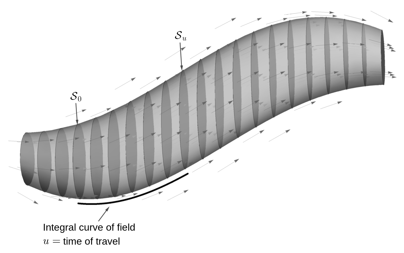
Figure 2.1. A channel generated by “sliding” a cross section $\mathcal{S}_{0}$ along the integral curves of a vector field. The wall $\mathcal{W}$ consists of the surface that encapsulates the channel, but not including the cross sections at its extreme sides.

We are interested in studying channel-like objects, which we will denote by $\mathcal{C}$, in an $n-$dimensional space $M$. We will construct $\mathcal{C}$ using the following procedure (see Figure 2.1). Let $\mathcal{S}_{0}$ be a $(n-1)$-dimensional hyper-surface with boundary in $M$ and let $\bm{U}$ a vector field in $\mathcal{C}$. For a given real number $u$, let $\SS_{u}$ be the hyper-surface obtained by “sliding” $\SS_{0}$ along the integral curves of $\bm{U}$ for a duration of $u$. We will refer to $\mathcal{S}_{u}$ as the cross section of $\mathcal{C}$ at $u$. If $\mathcal{C}$ is the union of the cross sections $\SS_{u}$, we will say that the vector field $\bm{U}$ generates $\mathcal{C}$. If $\partial\mathcal{S}_{u}$ is the boundary of $\mathcal{S}_{u}$, the wall $\mathcal{W}$ of $\mathcal{C}$ is the union of the sets $\partial\mathcal{S}_{u}$ for all $u$’s. For $x$ in $\mathcal{C}$ we will let $u(x)$ be equal to the time it takes for a point in $\mathcal{S}_{0}$ to reach $x$ (by following an integral curve of $\bm{U}$). In this context, we will refer to $u$ as a projection function for the channel. Notice that $\SS_{s}$ can be characterized as the set of points in $\mathcal{C}$ at which $u(x)=s$.

As a particular case of the above construction consider a parametric channel, obtained by using a parametrization function $x=x(u,\text{$v)$}$ where $u$ is a scalar and $v$ belongs to some region in $(n-1)$-dimensional space. In this case the generating vector field of the channel is

$$\bm{U}(x)=\frac{\partial x}{\partial u}(u(x),v(x)),$$

where $u(x)$ and $v(x)$ are the $u$ and $v$ coordinates of the point $x$ in $M$.

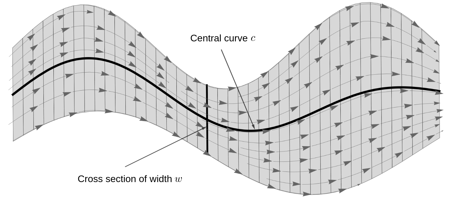
Figure 2.2. Parametric channel with central function $c=c(u)$ and width function $w=w(u)$.

Example 1.

For $n=2$ let the variable $v$ be in re region $-1/2\leq v\leq 1/2$ and define (see Figure 2.2)

$$x(u,v)=(u,c(u)+vw(u)),$$

for scalar valued functions $c=c(u)$ and $w=w(u)$. We have that

$$\frac{\partial x}{\partial u}(u,v)=(1,c^{\prime}(u)+vw^{\prime}(u)).$$

If we write $x=(x_{1},x_{2})$, then from the formulas

$$x_{1}=u\text{ and }x_{2}=c(u)+vw(u)$$

we obtain

$$v=\frac{x_{2}-c(x_{1})}{w(x_{1})}.$$

Hence, the generating vector field of the channel is

$$\bm{U}(x_{1},x_{2})=\left(1,c^{\prime}(x_{1})+\left(\frac{x_{2}-c(x_{1})}{w(x_{1})}\right)w^{\prime}(x_{1})\right).$$

A projection function for this field is

$$u(x_{1},x_{2})=x_{1},$$

and the cross section $\SS_{u}$ is a line parallel to the $x_{2}$-axis intersecting the $x_{1}$-axis at $(u,0)$.

Remark 2.

We constructed the projection function $u$ in terms the vector field $\bm{U}$, by letting $u(x)$ be the time it takes for an integral curve of $\bm{U}$ starting at $\SS_{0}$ to reach $x$. Alternatively, we could first select a scalar valued function $u$ in $\mathcal{C}$ and then construct a generating vector field $\bm{U}$ in $M$ that satisfies

$$\nabla u(x)\cdot\bm{U}(x)=1\text{ for all x in }\mathcal{C}.$$

This condition implies that $u$ is a projection function of for $\bm{U}$. The initial cross section $\SS_{0}$ is then chosen so that $u(x)=0$ for all $x$ in $\SS_{0}$.

2.1. Natural projection functions and fields

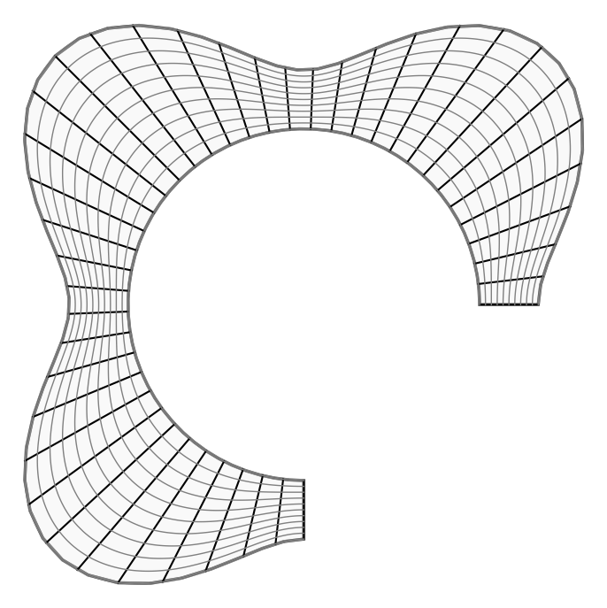
(a)

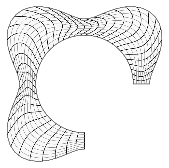
(b)

Figure 2.3. Two sets of cross sections associated with two different generating vector fields of the same channel.

A channel $\mathcal{C}$ can have many generating fields, which in general produce different sets of cross sections (see Figure 2.3 ). This observation leads to the following problem.

Problem 3.

Consider a channel $\mathcal{C}$ with two fixed cross sections $\mathcal{A}$ and $\mathcal{B}$. Is there a way to chose a generating vector field $\bm{U}$ for $\mathcal{C}$ such that $\mathcal{A}$ and $\mathcal{B}$ are cross sections of $\mathcal{C}$ generated by $\bm{U}$, and generated cross in between them “fit” the geometry of $\mathcal{C}$ in a “natural way”?

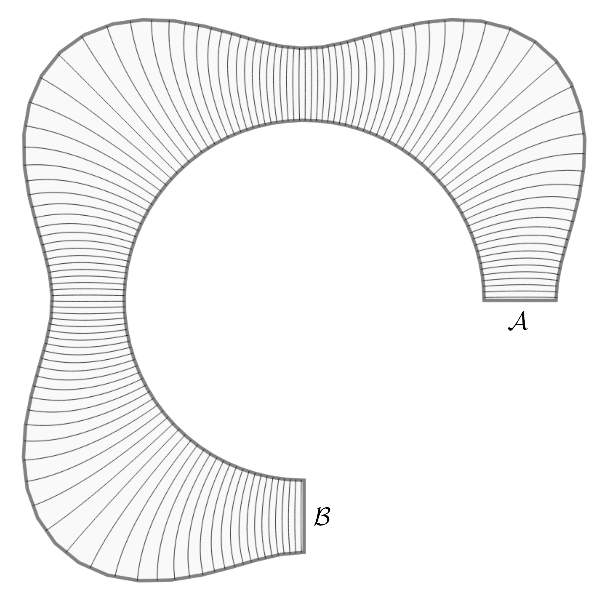
(a) Cross sections

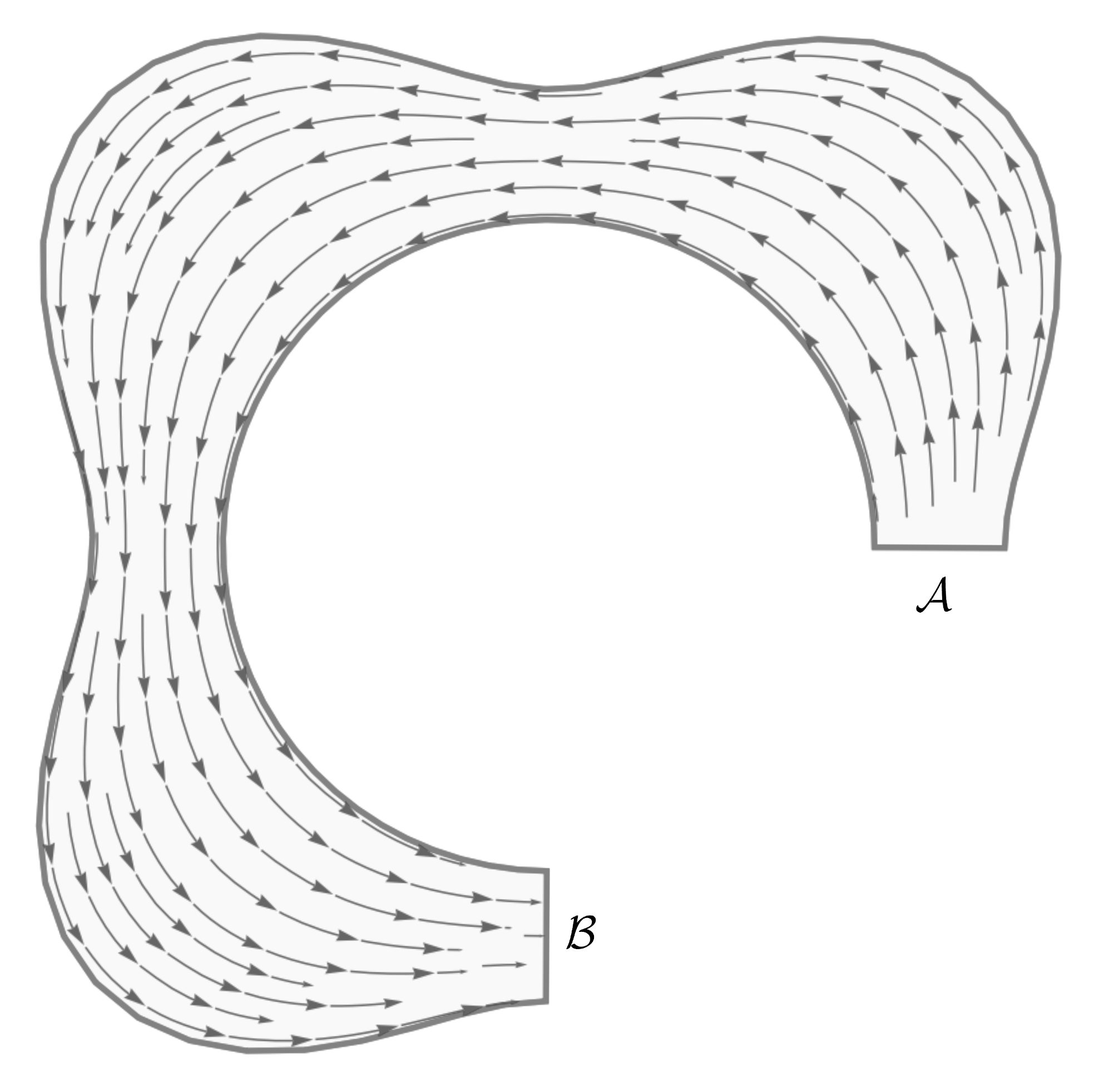
(b) Generating vector field

Figure 2.4. Cross sections and generating field associated to a harmonic function $h$ on a channel. This function takes the values $0$ and $1$ on $\mathcal{A}$ and $\mathcal{B}$ (respectively), and its gradient has no flux across the other walls of the channel (i.e in $\mathcal{W}$).

We will argue that a “natural way” to choose $\bm{U}$ is as follows. For two different scalars $a$ and $b$ let $h$ be a harmonic function (i.e $\Delta h=0)$ on $\mathcal{C}$ such that $\nabla h$ has no flux across $\mathcal{W}$, and satisfies the boundary conditions

(2.1) $$h(x)=\begin{cases}a&\text{ if }x\text{ is in }\mathcal{A},\\ b&\text{ if }x\text{ is in }\mathcal{B}.\end{cases}$$

We will let (see Figure 2.4) $\bm{U}=\bm{H}$, where

(2.2) $$\bm{H}(x)=\nabla h(x)/||\nabla h(x)||^{2}.$$

This field generates the channel $\mathcal{C}$ and has $h$ as projection function. We will refer to $h$ and $\bm{H}$ as a natural projection function and a natural generating field for the channel $\mathcal{C}$ with lateral cross sections $\mathcal{A}$ and $\mathcal{B}$.

Remark 4.

If we write $h=h_{a,b}$ to specify that $h$ takes the values $a$ and $b$ in $\mathcal{A}$ and $\mathcal{B}$, respectively, then we have that

$$h_{a,b}=a+(b-a)h_{0,1}.$$

2.2. Flux functions

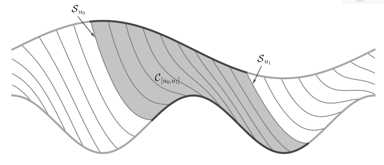
Figure 2.5. Channel region between two cross section

The flux function of a vector field $\bm{V}$ in channel $\mathcal{C}$ is defined as

$$\mathcal{F}_{\bm{V}}(u)=\text{flux of }\bm{V}\text{ across }\SS_{u}.$$

In the above definition we have assumed that we have fixed a generating vector field $\bm{U}$ for $\mathcal{C}$ (and hence its cross sections). The importance of the generating vector field $\bm{U}$ of a channel is that we will be able to express many quantities of interest in terms $\bm{U}$. In particular we will consider the flux functions of vector fields $\bm{V}$ of the form $\bm{V}=\lambda\bm{U}$, where $\lambda$ is a scalar valued function in $\mathcal{C}$. In this case we have that

$$\mathcal{F}_{\bm{V}}(u)=\frac{dc_{\lambda}}{du}(u),$$

where for (see Figure 2.5 )

$$\mathcal{C}_{[u_{0},u_{1}]}=\text{union of the sets }\mathcal{S}_{u}\text{ for }u_{0}\leq u\leq u_{1}$$

we defined

$$c_{\lambda}(u)=\text{total concentration of }\lambda\text{ in }\mathcal{C}_{[0,u]}.$$

Example 5.

Let

$$\nu(u)=\text{volume of }\mathcal{C}_{[0,u]}.$$

For $\lambda=1$ we have that $\nu(u)=c_{\lambda}(u)$, and hence

$$\frac{d\nu}{du}(u)=\mathcal{F}_{\bm{U}}(u).$$

An important property of the flux function, that we will use frequently, is that if we can write $\lambda=\lambda(u)$, then

$$\mathcal{F}_{\lambda V}(u)=\lambda(u)\mathcal{F}_{V}(u)$$

3. Effective diffusion on channels

For a given channel $\mathcal{C}$, we are interested in studying the evolution of a density function $P=P(x,t)$ that obeys the diffusion equation

$$\frac{\partial P}{\partial t}(x,t)=D_{0}\Delta P(x,t).$$

We will assume reflective boundary conditions on the wall $\mathcal{W}$ of $\mathcal{C}$, i.e the gradient of $P$ has no flux across $\mathcal{W}$. Using a projection function in $\mathcal{C}$, we will try to reduce the above equation to a diffusion equation in a $1$-dimensional spatial variable. To do this, we define the total concentration function as

$$c(u,t)=\text{total concentration of density }P\text{ in }\mathcal{C}_{[0,u]}\text{ at time }t.$$

and the volume function $\nu$ by

(3.1) $$\nu(u)=\text{volume of }\mathcal{C}_{[0,u]}.$$

We can now define the effective concentration as

$$p(u,t)=\frac{\partial c}{\partial u}(u,t)/\frac{d\nu}{du}(u).$$

If we let $u=u(\nu)$ be the value of $u$ that corresponds to volume $\nu$ and $p(\nu,t)=p(u(\nu),t)$, then

$$p(\nu,t)=\frac{\partial c}{\partial\nu}(\nu,t).$$

Hence, the total concentration of $P$ in the region $\mathcal{C}_{[u_{1},u_{2}]}$ at time $t$ is given by

$$\int_{\nu_{1}}^{\nu_{2}}p(\nu,t)d\nu\text{ for }\nu_{i}=\nu(u_{i}).$$

Remark 6.

In most of the literature the effective concentration is defined as

(3.2) $$p(u,t)=\frac{dc}{du}(u,t),$$

so that the total concentration of $P$ in $\mathcal{C}_{[u_{1},u_{2}]}$ is

$$\int_{u_{1}}^{u_{2}}p(u,t)du.$$

From a mathematical point of view the definition of the effective concentration 3.2 is not convenient for the following reason. If we introduce a new variable $v=v(u)$, with our definition of effective concentration we have that

$$p(u,t) =\frac{\partial c}{\partial u}(u,t)/\left(\frac{d\nu}{du}(u)\right)$$

$$=\left(\frac{\partial c}{\partial v}(v(u),t)\frac{dv}{du}(u)\right)/\left(\frac{d\nu}{dv}(v(u))\frac{dv}{du}(u)\right)$$

$$=\frac{\partial c}{\partial v}(v(u),t)\frac{d\nu}{dv}(v(u))$$

$$=p(v(u),t).$$

This is the proper formula for the change of variable of a function. On the other hand, if we define $p$ as in 3.2 we have

$$p(u,t)=\frac{dc}{du}(u,t)=\frac{d\nu}{du}(u)\frac{dc}{d\nu}(\nu(u),t)=\frac{d\nu}{du}(u)p(\nu(u),t),$$

which is the way vectors (not functions) transform under a change of variable.

3.1. Infinite transversal diffusion rate

If we assume that the density function $P$ stabilizes infinitely fast along the cross sections $\SS_{u}$ of $\mathcal{C}$, which is equivalent to $P$ being constant along them, we arrive at the effective diffusion equation (see Section 4.4)

(3.3) $$\frac{\partial p}{\partial t}(u,t)=\nabla\cdot(\mathcal{D}(u)\nabla p(u,t)),$$

where the effective diffusion coefficient is given by

(3.4) $$\mathcal{D}(u)=D_{0}\mathcal{F}_{\nabla u}(u)\frac{d\nu}{du}(u).$$

The divergence and gradient operators $\nabla\cdot$ and $\nabla$ in formula 3.3 are the ones associated to the metric

(3.5) $$g(u)=\left(\frac{d\nu}{du}(u)\right)^{2},$$

i.e

$$\nabla p=\frac{1}{g}\frac{\partial p}{\partial u}\text{ and }\nabla\cdot j=\frac{1}{\sqrt{g}}\frac{\partial}{\partial u}\left(\sqrt{g}j\right).$$

Observe that if we let $u=\nu$ then $g=1,$ and hence

$$\nabla p=\frac{\partial p}{\partial\nu},\nabla\cdot j=\frac{\partial j}{\partial\nu}$$

and

$$\mathcal{D}(\nu)=D_{0}\mathcal{F}_{\nabla\nu}.$$

Remark 7.

The effective diffusion coefficient $\mathcal{D}$ connects the effective flux

$$j(u,t)=\mathcal{F}_{J_{t}}(u)/\frac{d\nu}{du}(u)\text{ where }J_{t}=D_{0}\nabla P_{t}$$

with the gradient of the effective density function. More concretely, Fick’s first law establishes that (see sections 4.3 and 4.4)

$$j(u,t)=-\mathcal{D}(u)\nabla p(u,t).$$

Remark 8.

The condition of $P$ being constant along the cross sections of the channel implies that we can write (see Section 4.4)

$$P(x,t)=p(u(x),t),$$

where $p$ is the effective density function and $u$ is the projection function. If we had used the definition of effective concentration found in most of the literature, this identity would not hold.

Comparison with the generalized Fick-Jacobs equation

If we let

$$\sigma(u)=\frac{d\nu}{du}(u)\text{ and }p_{f}(u,t)=\frac{dc}{du}(u,t),$$

we can write equation 3.3 as a generalized Fick-Jacobs equation

$$\frac{dp_{f}}{dt}(u,t)=\frac{\partial}{\partial u}\left(\sigma(u)\mathcal{D}_{f}(u)\frac{\partial}{\partial u}\left(\frac{p_{f}(u,t)}{\sigma(u)}\right)\right),$$

where the effective diffusion coefficient is given by

$$\mathcal{D}_{f}(u)=\frac{D_{0}\mathcal{F}_{\nabla u}(u)}{\sigma(u)}.$$

If we define the effective flux $j_{f}$ as

$$j_{f}(u,t)=\mathcal{F}_{J_{t}}(u,t)$$

then we have the continuity equation (see 4.3)

$$\frac{\partial p_{f}}{\partial t}+\frac{\partial j_{f}}{\partial u}=0.$$

Using the Fick-Jacobs equation we conclude that

$$j_{f}=-\sigma\mathcal{D}_{f}\frac{\partial}{\partial u}\left(\frac{p_{f}}{\sigma}\right).$$

From these equations and the formulas

$$p=p_{f}/\sigma\text{ and }j=j_{f}/\sigma$$

we obtain

$$j(u,t)=-\mathcal{D}_{f}(u)\frac{\partial p}{\partial u}(u,t).$$

We conclude that the difference between the effective diffusion coefficient given by the generalized Fick-Jacobs equation and ours is that: in the first case the gradient used in Fick’s first law is that associated to the metric $g=1$, and in the second case it is that associated to the metric $g(u)=\sigma(u)^{2}$. The formula connecting both coefficients is

$$\mathcal{D}_{f}(u)=\frac{\mathcal{D}(u)}{\sigma(u)^{2}}.$$

Observe that when the cross sections of $\mathcal{C}$ are parametrized by the volume variable $\nu$, we have that $\sigma(\nu)=1$ and hence

$$\mathcal{D}_{f}(\nu)=\mathcal{D}(\nu)=D_{0}\mathcal{F}_{\nabla\nu}(\nu).$$

Furthermore, in this case both the effective diffusion equation and the Fick-Jacobs equation become the diffusion equation

$$\frac{\partial p}{\partial t}(\nu,t)=\frac{\partial}{\partial\nu}\left(\mathcal{D}(\nu)\frac{\partial p}{\partial\nu}(\nu,t)\right).$$

Cross section density function

If we define the area function as

$$\mathcal{A}(u)=\text{area of }\SS_{u}$$

and let

$$\mathcal{G}(u)=\frac{\mathcal{F}_{\nabla u}(u)}{\mathcal{A}(u)},$$

then we can write

$$\mathcal{D}(u)=D_{0}\mathcal{A}(u)\mathcal{G}(u)\frac{d\nu}{du}(u).$$

Since the cross sections $\mathcal{S}_{u}$ are the level sets of $u$, the vector field $\nabla u$ is orthogonal to them. Hence, if we orient the cross sections $\SS_{u}$ so that their normal fields have the same direction as $\nabla u$, we have that

$$\mathcal{G}(u)=\text{average value of }|\nabla u|\text{ on }\mathcal{S}_{u}.$$

This number measures the average density of cross sections near $\SS_{u}$, and we will refer to $\mathcal{G}$ as the cross section density function. If the cross sections of the channel are parametrized by the volume variable $\nu$, we have that

$$\mathcal{D}(\nu)=D_{0}\mathcal{A}(\nu)\mathcal{G}(\nu).$$

3.2. Finite transversal diffusion rate

Consider a channel $\mathcal{C}$ whose cross sections $\mathcal{S}_{u}$ are generated by a vector field $\bm{U}$, and let us drop the assumption that the density function $P=P(x,t)$ stabilizes infinitely fast along these cross sections. To give a formula for the effective diffusion coefficient $\mathcal{D}=\mathcal{D}(u)$, we will make use of the natural projection function $h$ and the natural generating field $\bm{H}$ of the channel $\mathcal{C}$ with lateral cross sections $\SS_{u_{0}}$ and $\SS_{u_{1}}$ for $u_{0}<u_{1}$(see section 2.1). In this context, we will refer to the projection function $u$ and the field $\bm{U}$ as the imposed projection function and field (to distinguish them from the natural ones: $h$ and $\bm{H}$).

Let $\rho$ be the effective density function of $h$ under the projection map $u$, i.e

$$\rho(u)=\mathcal{F}_{hU}(u)/\frac{d\nu}{du}(u).$$

In section 4.5 we proved that (for $u$ with $u_{0}\leq u\leq u_{1}$) the effective diffusion coefficient $\mathcal{D}$ appearing in formula 3.3 can be computed as

(3.6) $$\mathcal{D}(u)=\mathcal{J}\left(\frac{d\nu}{du}(u)\right)^{2}/\mathcal{F}_{\lambda U}(u),$$

where $\lambda=\lambda(x)$ is a scalar valued function in $\mathcal{C}$ defined by

(3.7) $$\lambda=\nabla h\cdot U+(h-\rho\circ u)\nabla\cdot U$$

and the constant $\mathcal{J}$ is given by

$$\mathcal{J}=D_{0}\mathcal{F}_{\nabla h}(u_{0}).$$

Channels with natural projection map

If for a given channel $\mathcal{C}$ we choose the imposed projection map an generating vector field to be the natural ones, i.e

$$\bm{U}=\bm{H}\text{ and }u=h,$$

then we have that

$$\nabla h\cdot U=\frac{\nabla h\cdot\nabla h}{||\nabla h||^{2}}=1.$$

and

$$\rho(u(x)) =\mathcal{F}_{hU}(u(x))/\frac{d\nu}{du}(u(x))$$

$$=h(x)\mathcal{F}_{U}(u(x))/\frac{d\nu}{du}(u(x))$$

$$=h(x),$$

where we have made use of the formula

$$\frac{d\nu}{du}(u)=\mathcal{F}_{U}(u).$$

Hence $\lambda=1$ in formula 3.7, which implies

$$\mathcal{D}(u)=\mathcal{J}\left(\frac{d\nu}{du}(u)\right)^{2}\left(\mathcal{F}_{U}(u)\right)^{-1}=D_{0}\mathcal{F}_{\nabla u}(u)\frac{d\nu}{du}(u).$$

We conclude that when using the natural projection function and field of a channel, the formulas for the effective diffusion coefficient in the finite and infinite diffusion transversal rate cases coincide.

4. Derivation of the effective diffusion coefficient formula

Let $M$ be an oriented Riemannian manifold of dimension $n$. We are interested in the diffusion equation

$$\frac{\partial P}{\partial t}(x,t)=\nabla\cdot(D(x)\nabla P(x,t)),$$

where $P:M\times\mathbb{R}\rightarrow\mathbb{R}$ is a time dependent function in $M$ and $D(x):T_{x}X\rightarrow T_{x}X$ is a linear map for every $x$ in $M$. The divergence and gradient operators in the above formula can defined in terms of exterior algebra operations as

$$\nabla\cdot J=*d*J^{\flat}\text{ and }\nabla P=(dP)^{\#},$$

where $d:\bigwedge^{k}M\rightarrow\bigwedge^{k+1}M$ is the exterior derivative, $*:\bigwedge^{k}M\rightarrow\bigwedge^{n-k}M$ the Hodge star operator, and the musical isomorphisms $\sharp$ and $\flat$ allow us to identify 1-forms and vector fields. If we let $g$ stand for the metric tensor in $M$ and use local coordinates $x_{1},\ldots x_{n}$, we can write

$$\nabla\cdot J=\frac{1}{|g|^{1/2}}\sum_{i=1}^{n}\frac{\partial}{\partial x_{i}}\left(|g|^{1/2}J_{i}\right)\text{ where }|g|=\det(g)$$

and

$$(\nabla P)^{i}=\sum_{j=1}^{n}g^{ij}\frac{\partial P}{\partial x_{j}}\text{ where }(g^{ij})=(g_{ij})^{-1}.$$

.

In a homogeneous and isotropic medium the diffusion has the form

(4.1) $$\frac{\partial P}{\partial t}(x,t)=D_{0}\Delta P(x,t)\text{ where }\Delta=*d*d\text{ and }D_{0}\in\mathbb{R}.$$

4.1. Channels and projection functions

Let $M$ be an $n$-dimensional oriented Riemannian manifold. We will say that $\mathcal{C}\subset M$ is generated by a vector field $U$, if $\mathcal{C}$ is the union of phase curves of $U$ that have transversal intersection with an $(n-1)$-dimensional sub-manifold with boundary $\SS_{0}$. We will then say that $\mathcal{C}$ is a channel generated by $U$ having $\mathcal{S}_{0}$ as an initial cross section. A smooth function $u:\mathcal{C}\rightarrow\mathbb{R}$ is a projection function for the field $U$ if $du(U)=1$. We will usually choose $\mathcal{S}_{0}$ so that $\mathcal{S}_{0}=u^{-1}(0)$. The cross section $\mathcal{S}_{s}$ of $\mathcal{C}$ at $s$ is defined by the formula

$$\mathcal{S}_{s}=u^{-1}(s).$$

Recall that the phase flow $\{\varphi_{s}:\mathcal{C}\rightarrow\mathcal{C}\}_{s\in\mathbb{R}}$ of $U$ is defined by

$$\left.\frac{d}{ds}\right|_{s=0}(\varphi_{s}(x))=U(x),$$

and satisfies

(4.2) $$\varphi_{s_{1}+s_{2}}=\varphi_{s_{1}}\circ\varphi_{s_{2}}.$$

The condition $du(U)=1$ is then equivalent to

$$u(\varphi_{s}(x))=u(x)+s,$$

and hence

$$\mathcal{S}_{s+h}=\varphi_{h}(\mathcal{S}_{s}).$$

If we let $\mathcal{W}=\partial\mathcal{C}$ then $\mathcal{W}$ is the union of phase curves of $U$ that intersect $\partial\mathcal{S}_{0}$. We will refer to $\mathcal{W}$ as the reflective wall of $\mathcal{C}$. We define

$$\mathcal{C}_{[s_{1},s_{2}]}=u^{-1}([s_{1},s_{2}])\text{ and }\mathcal{W}_{[s_{1},s_{2}]}=\mathcal{W}\cap\mathcal{C}_{[s_{1},s_{2}]}.$$

Flux functions

We will let $\mu\in\bigwedge^{n}M$ stand for global volume form associated with the metric in $M$. The orientation in $\mathcal{C}$ will the the one induced by the orientation of $M$, i.e we will let the orientation form be the one obtained by restricting $\mu$ to $\mathcal{C}$. Observe that

(4.3) $$du\wedge\iota_{U}(\mu)=du\wedge(*U^{\flat})=<du,U^{\flat}>\mu=du(U)\mu=\mu.$$

If we let $i_{u}:\mathcal{S}_{u}\rightarrow\mathcal{C}$ be the inclusion map then $i_{u}^{*}(\iota_{U}(\mu))$ is an $(n-1)$-form in $\mathcal{S}_{u}$ which vanishes no-where in $\mathcal{S}_{u}$. We will use this form as an orientation form for $\SS_{u}$. For a vector field $V$ in $\mathcal{C}$ we define the flux function $\mathcal{F}_{V}:\mathbb{R}\rightarrow\mathbb{R}$ as

$$\mathcal{F}_{V}(u)=\int_{\SS_{u}}\iota_{V}(\mu)=\int_{\mathcal{S}_{u}}*(V^{\flat}).$$

In particular

$$\mathcal{F}_{\nabla P}(u)=\int_{\mathcal{S}_{u}}*(dP).$$

Change of variable formulas

Let $u:\mathcal{C}\rightarrow\mathbb{R}$ be a projection function for $U$ and $f:\mathbb{R}\rightarrow\mathbb{R}$ a function with positive derivative. If we let $v=f\circ u$ then

$$dv(x)=f^{\prime}(u(x))du(x),$$

which implies that $v$ is a projection function for the field $V$ defined by $V(x)=U(x)/f^{\prime}(u(x))$. To simplify notation, we will write the conditions $v=f\circ u$ and $u=f^{-1}\circ v$ as

$$v=v(u)\text{ and }u=u(v),$$

where in the first equation $u$ is seen as a scalar value and $v$ as a function, and on the second formula $v$ is seen as a scalar value and $u$ as a function. If we denote a cross sections at $u$ as $\mathcal{S}_{u}$ and a cross section at $v$ as $\SS_{v}$, then the formulas $u^{-1}(s)=v^{-1}(f(s))$ and $v^{-1}(s)=u^{-1}(f^{-1}(s))$ can be simply written as $\mathcal{S}_{u}=\SS_{v(u)}$ and $\SS_{v}=\SS_{u(v)}$. Furthermore, we have that

(4.4) $$dv=\left(\frac{dv}{du}\right)du\text{ and }V=\left(\frac{dv}{du}\right)^{-1}U,$$

where

$$\frac{dv}{du}(x)=f^{\prime}(u(x)).$$

Remark 9.

If for a positive function $\lambda:\mathbb{R}\rightarrow\mathbb{R}$ we let $V=(\lambda\circ u)U$, then we can recover the projection function $v=v(u)$ for $V$ as

$$v(u)=v_{0}+\int_{u_{0}}^{u}\left(\frac{1}{\lambda(s)}\right)ds\text{ for }v_{0}\in\mathbb{R}.$$

4.2. Some useful identities

We will now derive some identities that will be useful in our study of diffusion processes on channels. Let $\mathcal{C}$ be a channel generated by a field $U$ and with a projection function $u$. In what follows we will make use of Cartan’s magic formula

$$\mathcal{L}_{U}=\iota_{U}\circ d+d\circ\iota_{U},$$

where $\mathcal{L}_{U}$ is the Lie derivative with respect to $U$.

Lemma 10.

If $\alpha$ is an $(n-1)$-form in $\mathcal{C}$ and we define

$$f(u)=\int_{S_{u}}\alpha,$$

then

$$f^{\prime}(u)=\int_{S_{u}}\mathcal{L}_{U}\alpha.$$

If $\omega$ is an $n$-form in $\mathcal{C}$ and for any $u_{0}\in\text{$\mathbb{R}$}$ we define

$$g(u)=\int_{\mathcal{C}_{[u_{0},u]}}\omega$$

then

$$g^{\prime}(u)=\int_{S_{u}}\iota_{U}(\omega)$$

and

$$g^{\prime\prime}(u)=\int_{S_{u}}\left(d\lambda(U)+\lambda\nabla\cdot U\right)\iota_{U}(\mu)\text{ where }\lambda=*\omega.$$

Proof.

From the formula $S_{u+h}=\varphi_{h}(S_{u})$ we obtain

$$f(u+h)-f(u)=\int_{S_{u+h}}\alpha-\int_{S_{u}}\alpha=\int_{S_{u}}(\varphi_{h}^{*}\alpha-\alpha),$$

and hence

$$f^{\prime}(u)=\lim_{h\mapsto 0}\int_{S_{u}}\frac{1}{h}(\varphi_{h}^{*}(\alpha)-\alpha)=\int_{S_{u}}\mathcal{L}_{U}\alpha.$$

To prove the second part of the lemma observe that

$$g(u+h)-g(u)=\int_{\mathcal{C}_{[u,u+h]}}\omega,$$

and hence

$$g^{\prime}(u)=\lim_{h\mapsto 0}\frac{g(u+h)-g(u)}{h}=\lim_{h\mapsto 0}\frac{1}{h}\int_{u}^{u+h}\int_{\mathcal{S}_{t}}(\iota_{U}(\omega))dt=\int_{\mathcal{S}_{u}}\iota_{U}(\omega).$$

Combining the previous results we obtain

$$g^{\prime\prime}(u)=\int_{S_{u}}\mathcal{L}_{U}(\iota_{U}(\omega)).$$

Using Cartan’s magic formula it is easy to verify that

$$\mathcal{L}_{U}(\iota_{U}(\omega))=\iota_{U}(\mathcal{L}_{U}(\omega)).$$

We can write $\omega=\lambda\mu$ for $\lambda=*\omega$, and hence

$$\mathcal{L}_{U}(\omega)=\mathcal{L}_{U}(\lambda\mu)=\iota_{U}(d\lambda)\mu+\lambda\mathcal{L}_{U}\mu.$$

Using this and the fact that $\mathcal{L}_{U}\mu=(\nabla\cdot U)\mu$, we conclude that

$$\iota_{U}(\omega)=(d\lambda(U)+\lambda(\nabla\cdot U))\iota_{U}(\mu)$$

∎

4.3. The effective continuity equation

If we let the metric tensor in the $u$ variable be

$$g(u)=\left(\frac{d\nu}{du}(u)\right)^{2},$$

then the divergence and gradient operators are given by the formulas

$$\nabla\cdot j=g^{-1/2}\frac{\partial}{\partial u}\left(g^{1/2}j\right)\text{ and }\nabla p=g^{-1}\frac{\partial p}{\partial u}.$$

Consider a concentration function $P=P(x,t)$ and the flux vector field $J=J(x,t)$. Let us write $P_{t}(x)=P(x,t)$ and $J_{t}(x)=J(x,t)$, and for a channel $\mathcal{C}$ define the effective flux function as

$$j(u,t)=\mathcal{F}_{J_{t}}(u)/\frac{d\nu}{du}(u)\text{ where }\mathcal{F}_{J_{t}}=\int_{\mathcal{S}_{u}}*J_{t}^{\flat}.$$

and the effective concentration as

$$p(u,t)=\frac{\partial c}{\partial u}(u,t)/\frac{d\nu}{du}(u)\text{ where }c(u,t)=\int_{\mathcal{C}_{[0,u]}}*P_{t}.$$

By Lemma 10 we have that

$$\frac{\partial c}{\partial u}(u,t)=\int_{\mathcal{S}_{u}}\iota_{U}(*P_{t})$$

and

$$\frac{d\mathcal{F}_{J_{t}}}{du}(u)=\int_{\SS_{u}}\mathcal{L}_{U}(*J_{t}^{\flat})=\int_{\SS_{u}}(d\circ\iota_{U}+\iota_{U}\circ d)(*J_{t}^{\flat}).$$

If we assume reflective boundary conditions on the wall $\mathcal{W}$ of $\mathcal{C}$, we get

$$\int_{S_{u}}d(\iota_{U}(*J_{t}^{\flat}))=\int_{\partial S_{u}}\iota_{U}(*J_{t}^{\flat})=0.$$

Using the above formulas and the continuity equation

$$*\frac{\partial P}{\partial t}(x,t)+d*J^{\flat}(x,t)=0$$

we obtain

$$\frac{d\mathcal{F}_{J_{t}}}{du}(u)=\int_{S_{u}}(\iota_{U}\circ d)(*J_{t}^{\flat})=-\int_{S_{u}}\iota_{U}\left(*\frac{\partial P}{\partial t}\right),$$

and hence

$$\int_{S_{u}}\iota_{U}\left(*\frac{\partial P}{\partial t}\right)=\frac{\partial}{\partial t}\int_{S_{u}}\iota_{U}(*P_{t})=\frac{\partial}{\partial t}\left(\frac{\partial c}{\partial u}(u,t)\right).$$

We conclude that

$$\frac{\partial}{\partial t}\left(\frac{\partial c}{\partial u}(u,t)\right)+\frac{d\mathcal{F}_{J_{t}}}{du}(u)=0,$$

which implies that

$$\frac{\partial}{\partial t}\left(g^{-1/2}(u)\frac{\partial c}{\partial u}(u,t)\right)+g^{-1/2}(u)\frac{\partial}{\partial u}\left(g^{1/2}(u)g^{-1/2}(u)\frac{d\mathcal{F}_{J_{t}}}{du}(u)\right)=0.$$

This last equation is known effective continuity equation and can be re-written as

(4.5) $$\frac{\partial p}{\partial t}(u,t)+\nabla\cdot j(u,t)=0.$$

4.4. Infinite transversal diffusion rate

The assumption of an infinite transversal diffusion rate is expressed mathematically by letting

$$P(x,t)=\rho(u(x),t)$$

for a function $\rho:\mathbb{R}\times\mathbb{R}\rightarrow\mathbb{R}$. The effective density function can then be written as

$$p(u,t)=g(u)^{-1/2}\int_{S_{u}}u^{*}(\rho_{t})\iota_{U}\mu=\rho(u,t)g(u)^{-1/2}\int_{S_{u}}\iota_{U}(\mu).$$

From the formula

$$\int_{S_{u}}\iota_{U}(\mu)=\frac{d\nu}{du}(u)=g(u)^{1/2},$$

we conclude that

$$p(u,t)=\rho(u,t).$$

Using Fick’s law $J_{t}=-D_{0}\nabla P_{t}$, we obtain

$$\mathcal{F}_{J_{t}}(u)=\int_{S_{u}}*J_{t}^{\flat}=-D_{0}\int_{S_{u}}*(dP_{t})=-D_{0}\int_{S_{u}}*(u^{*}(d\rho_{t})).$$

Since (for $s$ equal to the identity map in $\mathbb{R}$)

$$u^{*}(d\rho_{t})=u^{*}\left(\frac{\partial\rho_{t}}{\partial s}ds\right)=u^{*}\left(\frac{\partial\rho_{t}}{\partial s}\right)du,$$

we obtain

$$\mathcal{F}_{J_{t}}(u)=-D_{0}\frac{\partial\rho}{\partial u}(u,t)\int_{S_{u}}*(du).$$

Using this last formula and the fact that $\rho=p$, we obtain

$$j(u,t)=g(u)^{-1/2}\mathcal{F}_{J_{t}}(u)=-\left(D_{0}g(u)^{1/2}\int_{S_{u}}*(du)\right)g(u)^{-1}\frac{\partial p}{\partial u}(u,t).$$

Substitution of this formula for $j$ in the effective continuity equation 4.5 leads to the effective diffusion formula

(4.6) $$\frac{\partial p}{\partial t}(u,t)=\nabla\cdot(\mathcal{D}(u)\nabla p(u,t)),$$

where the effective diffusion coefficient is given by

$$\mathcal{D}(u) =D_{0}\left(\int_{S_{u}}*(du)\right)g(u)^{1/2}.$$

$$=D_{0}\mathcal{F}_{\nabla u}(u)\frac{d\nu}{du}(u).$$

4.5. Finite transversal diffusion rate

We will now consider the case when density function $P=P(x,t)$ is not necessarily constant along the cross sections of the channel. In general it is not possible to define define $\mathcal{D}=\mathcal{D}(u)$ such that the effective density function $p=p(u,t)$ satisfies the $1$-dimensional diffusion equation 4.6 exactly, but for many cases of narrow channels it is possible to find $\mathcal{D}$ such that $p$ satisfy 4.6 to a very good approximation. In any case, if such a $\mathcal{D}$ existed we could recover it from of a stable solution $\rho=\rho(u)$ to 4.6. In fact, if $\rho$ is such a function we have that

$$\nabla\cdot(\mathcal{D}\nabla\rho)=0,$$

which is equivalent to

(4.7) $$\frac{\partial}{\partial u}\left(\frac{\mathcal{D}}{\sigma}\frac{d\rho}{du}\right)=0\text{ where }\sigma=g^{1/2}=\frac{d\nu}{du}.$$

Hence, we can find a constant $\mathcal{J}\in\mathbb{R}$ such that

(4.8) $$\mathcal{D}(u)=\mathcal{J}\sigma(u)\left(\frac{d\rho}{du}(u)\right)^{-1}.$$

Remark 11.

If we introduce a new variable $v=v(u)$, then we have that

$$\mathcal{D}(v)=\mathcal{D}(u(v)),$$

since

$$\mathcal{D}(v) =\mathcal{J}\frac{d\nu}{dv}(v)\left(\frac{d\rho}{dv}(v)\right)^{-1}$$

$$=\mathcal{J}\frac{d\nu}{du}(u(v))\frac{du}{dv}(v)\left(\frac{d\rho}{du}(u(v))\frac{du}{dv}(v)\right)^{-1}$$

$$=\mathcal{D}(u(v)).$$

We will now assume that $\rho$ is the effective concentration function of a stable solution $h=h(x)$ to the full diffusion equation 4.1 (with reflective boundary conditions on $\mathcal{W}$). We then have that

$$\rho(u)=\frac{1}{\sigma(u)}\int_{\mathcal{S}_{u}}h\iota_{U}(\mu)=\frac{1}{\sigma(u)}\frac{dc}{du}(u)$$

for

$$c(u)=\int_{\mathcal{C}_{[0,u]}}h\mu,$$

and hence

$$\frac{d\rho}{du}=\frac{d}{du}\left(\frac{1}{\sigma}\frac{dc}{du}\right)=\frac{1}{\sigma}\left(\frac{d^{2}c}{du^{2}}-\rho\frac{d^{2}\nu}{du^{2}}\right).$$

Using Lemma 10 we obtain

$$\frac{d^{2}c}{du^{2}}=\int_{\mathcal{S}_{u}}(dh(U)+h\nabla\cdot U)\iota_{U}(\mu),$$

and since

$$\nu(u)=\int_{\mathcal{C}_{[0,u]}}\mu$$

then

$$\frac{d^{2}\nu}{du^{2}}=\int_{\mathcal{S}_{u}}(\nabla\cdot U)\iota_{U}(\mu).$$

We conclude that

$$\mathcal{D}(u)=\mathcal{J}\sigma^{2}(u)/\mathcal{F}_{\lambda\bm{U}}(u)=\mathcal{J}\mathcal{F}_{\bm{U}}(u)\left(\frac{\mathcal{F}_{U}(u)}{\mathcal{F}_{\lambda U}(u)}\right)$$

where

$$\lambda=dh(U)+(h-u^{*}(\rho))\nabla\cdot U.$$

Computation of $\mathcal{J}$

By definition, we have

$$\mathcal{J}(u)=\frac{\mathcal{D}(u)}{\sigma(u)}\frac{d\rho}{du}(u).$$

Using Fick’s laws

$$j(u) =-\mathcal{D}(u)\nabla\rho(u)$$

$$J(x) =-D_{0}\nabla h(x)$$

and the formulas

$$j(u) =\frac{1}{\sigma(u)}\int_{\mathcal{S}_{u}}*J^{\flat}$$

$$\nabla\rho(u) =\frac{1}{\sigma(u)^{2}}\frac{d\rho}{du}(u)$$

we obtain

$$\mathcal{J}(u)=D_{0}\int_{\mathcal{S}_{u}}*(dh)=D_{0}\mathcal{F}_{\nabla h}(u).$$

The function $\mathcal{J}=\mathcal{J}(u)$ is in fact a constant function (i.e independent of $u$), since for any two values $u_{1}$ and $u_{2}$ we have that (by Stokes Theorem and the reflective boundary conditions on $\mathcal{W})$

$$\mathcal{J}(u_{2})-\mathcal{J}(u_{1})=D_{0}\int_{S_{u_{2}}-S_{u_{1}}}(*dh)=\int_{\mathcal{C}_{[u_{1},u_{2}]}}d*dh=\int_{\text{$\mathcal{C}$}_{[u_{1},u_{2}]}}*\Delta h=0.$$

Lateral boundary conditions

It is important to notice that formula 4.8 holds only under the assumption that $\rho^{\prime}(u)\not=0$ for all $u\in\mathbb{R}$. We can achieve this if for $\alpha\not=\beta$ we fix boundary the conditions

(4.9) $$\rho(a)=\alpha\text{ and }\rho(b)=\beta.$$

For fixed values of $\alpha$ and $\beta$ we will denote the stable solution to 4.6 satisfying these boundary conditions by $\rho_{\alpha,\beta}$. Using the linearity of equation 4.7 we obtain

$$\rho_{\alpha,\beta}=\alpha+(\beta-\alpha)\rho_{0,1}.$$

If we denote the constant $\mathcal{J}$ associated to $\rho_{\alpha,\beta}$ by $\mathcal{J}(\alpha,\beta)$ then

$$\mathcal{D}=\sigma\mathcal{J}(\alpha,\beta)\left(\frac{d\rho_{\alpha,\beta}}{du}\right)^{-1}.$$

Since $\mathcal{D}$ is independent of the choice of $\alpha$ and $\beta$ we must have

$$\mathcal{J}(\alpha,\beta)\left(\frac{d\rho_{\alpha,\beta}}{du}\right)^{-1}=\mathcal{J}(0,1)\left(\frac{d\rho_{0,1}}{du}\right)^{-1},$$

from which we obtain the formula

$$\mathcal{J}(\alpha,\beta)=(\beta-\alpha)\mathcal{J}(0,1).$$

The boundary conditions 4.9 can be written in terms of $H$ (using Lemma 10) as

$$\frac{1}{\sigma(a)}\int_{\mathcal{S}_{a}}h\iota_{U}(\mu) =\alpha,$$

$$\frac{1}{\sigma(b)}\int_{\mathcal{S}_{b}}h\iota_{U}(\mu) =\beta.$$

If we choose $h$ so that it is has constant value $h_{a}$ in $\SS_{a}$ and constant value $h_{b}$ in $\SS_{b}$, the above conditions become

$$h_{a}=\alpha\text{ and }h_{b}=\beta.$$

4.6. Channels defined by harmonic conjugate functions

Let $M$ be a 2-dimensional oriented surface. We will say that $u,v:M\rightarrow\mathbb{R}$ are harmonic conjugate if

$$dv=*du,$$

or equivalently

$$\nabla v=i\nabla u.$$

Observe that in this case

$$*dv=**du=-du.$$

The existence of a harmonic conjugate $v$ for $u$ implies that $u$ and $v$ are harmonic, since

$$\Delta u =*d*du=*(d^{2}v)=0,$$

$$\Delta v =*d*dv=-*(d^{2}u)=0.$$

For fixed value $v_{1},v_{2}\in\mathbb{R}$, consider a channel $\mathcal{C}$ defined as

$$\mathcal{C}=\{x\in M|v_{1}\leq v(x)\leq v_{2}\},$$

If we use a harmonic conjugate $u$ of $v$ as projection function for this channel, then $u$ is a harmonic function with reflective boundary conditions on $\mathcal{W}$. The channels $\mathcal{C}$ has generating field

$$U=\frac{\nabla u}{|\nabla u|^{2}}.$$

The effective diffusion coefficient both in the infinite and finite transversal diffusion rate cases coincide and is given by the formula

$$\mathcal{D}(u)=\mathcal{J}\frac{d\nu}{du}(u),$$

where

$$\mathcal{J}=\int_{\mathcal{S}_{u}}*du=\int_{\mathcal{S}_{u}}dv=v_{2}-v_{1}$$

and

$$\frac{d\nu}{du}(u)=\int_{\mathcal{S}_{u}}\frac{*du}{|\nabla u|^{2}}=\int_{\mathcal{S}_{u}}\frac{dv}{|\nabla v|^{2}}.$$

Observe that we can parametrize a cross section $\SS_{u}$ with a curve $x:[t_{1},t_{2}]\rightarrow\mathcal{C}$ with

$$\dot{x}(t)=\nabla v(x(t)),$$

so that

$$\mathcal{A}(u)=\int_{t_{1}}^{t_{2}}|\dot{x}(t)|=\int_{t_{1}}^{t_{2}}\frac{|\nabla v(x(t))|^{2}}{|\nabla v(x(t)|}.$$

Hence

$$\mathcal{A}(u)=\int_{\SS_{u}}\frac{dv}{|\nabla v|}.$$

4.7. Parametric channels

In this section we will assume that the channel $\mathcal{C}\subset M$ can be parametrized by a map

$$\varphi:[a,b]\times\Omega\rightarrow M,$$

where $\Omega$ is a $(n-1)$-dimensional sub-manifold with boundary of $\mathbb{R}^{n-1}$. In local coordinates we will write the elements of $[a,b]\times\Omega$ as $(u,v)$ for $u\in[a,b]$ and $v=(v_{1},\ldots,v_{n-1})\in\mathbb{R}^{n-1}$. If denote the of points in $\mathcal{C}$ by $x$ then we have that $x=\varphi(u,v)$, which we will simply write as $x=x(u,v)$. We will let the generating vector field for $\mathcal{C}$ be

$$U=\varphi_{*}\left(\frac{\partial}{\partial u}\right),$$

which has $u$ as a projection function. To compute the effective diffusion coefficient for $\mathcal{C}$ (in both the finite and infinite transversal diffusion rate cases) we will need to compute

$$\frac{d\nu}{du},\mathcal{F}_{\nabla u},\rho,dh(U)\text{ and }\nabla\cdot U,$$

where $h$ is a natural projection function for $\mathcal{C}$ and $\rho$ its corresponding effective density function. To compute the above quantities in $(u,v)$-coordinates we will make use of the metric tensor $g=\varphi^{*}(g_{M})$, where $g_{M}$ is the metric in $M$. We have that

$$g=\left(\begin{array}[]{cc}\text{$\frac{\partial x}{\partial u}\text{$\cdot\frac{\partial x}{\partial u}$}$}&\frac{\partial x}{\partial u}\cdot\frac{\partial x}{\partial v}\\ \left(\frac{\partial x}{\partial u}\cdot\frac{\partial x}{\partial v}\right)^{T}&g_{v}\end{array}\right),$$

where

$$\frac{\partial x}{\partial u}\cdot\frac{\partial x}{\partial v}=\left(\frac{\partial x}{\partial u}\cdot\frac{\partial x}{\partial v_{1}},\ldots,\frac{\partial x}{\partial u}\cdot\frac{\partial x}{\partial v_{n-1}}\right)$$

and $g_{v}$ is the matrix with entries

$$(g_{v})_{i,j}=\frac{\partial x}{\partial v_{i}}\cdot\frac{\partial x}{\partial v_{j}}.$$

The volume form in $\mathcal{C}$ is given by

$$\mu=\det(g)^{1/2}du\wedge dv,$$

and hence

$$\frac{d\nu}{du}(u) =\int_{\Omega}\iota_{\frac{\partial}{\partial u}}(\mu)=\int_{\Omega}\det(g(u,v))^{1/2}dv$$

$$\mathcal{A}(u) =\int_{\Omega}\det(g_{v}(u,v))^{1/2}dv$$

Observe that

$$\nabla u=a_{0}\frac{\partial}{\partial u}+\sum_{i=1}^{n-1}a_{i}\frac{\partial}{\partial v_{i}}$$

where

$$\left(\begin{array}[]{c}a_{0}\\ a_{1}\\ \vdots\\ a_{n-1}\end{array}\right)=g^{-1}\left(\begin{array}[]{c}1\\ 0\\ \vdots\\ 0\end{array}\right).$$

Since

$$a_{0}=\frac{\det(g_{v})}{\det(g)},$$

we conclude that

$$\mathcal{F}_{\nabla u}(u) =\int_{\Omega}\det(g(u,v))^{\frac{1}{2}}\iota_{\nabla u}(du\wedge dv)$$

(4.10) $$=\int_{\Omega}\left(\frac{\det(g_{v}(u,v))}{\det(g(u,v))^{\frac{1}{2}}}\right)dv.$$

The divergence of $U$ can be computed using the the formula $d(\iota_{U}(\mu))=(\nabla\cdot U)\mu$. In our case we have that

$$d(\iota_{U}(\mu))=d(\det(g)^{1/2}dv)=\frac{\partial\det(g)^{1/2}}{\partial u}du\wedge dv,$$

and hence

$$\nabla\cdot U=\frac{\frac{\partial}{\partial u}\left(\det(g)^{1/2}\right)}{\det(g)^{1/2}}=\frac{1}{2}\frac{\partial}{\partial u}\left(\log(\det(g))\right).$$

If $h$ is the natural projection map on the channel then

$$dh(U)=\frac{\partial h}{\partial u}$$

and

$$\rho=\left(\int_{\Omega}h(u,v)\det(g(u,v))^{1/2}dv\right)/\left(\int_{\Omega}\det(g(u,v))^{1/2}dv\right)$$

References

- [1] R.M. Bradley. Diffusion in a two-dimensional channel with curved midline and varying width. Phys. Rev. E, B 80, 2009.
- [2] C.Valero and R.Herrera. Fick-jacobs equation for channels over three-dimensional curves. Phy, 90(052141), 2014.
- [3] Yariv E. & Brenner H. Curvature-induced dispersion in electro-osmotic serpentine flows. SIAM J. Appl. Mathe, 64-4, 2004.
- [4] P. Kalinay and K. Percus. Extended fick-jacobs equation: Variational approach. Physical Review E, 72, 2005.
- [5] P. Kalinay and K. Percus. Projection of a two-dimensional diffusion in a narrow channel onto the longitudinal dimension. The Journal of Chemical Physics, 122, 2005.
- [6] P. Kalinay and K. Percus. Corrections to the fick-jacobs equation. Physical Review E, 74, 2006.
- [7] P. Kalinay and K. Percus. Aproximations to the generalized fick-jacobs equation. Physical Review E, 78, 2008.
- [8] N. Ogawa. Diffusion in a curved cube. Physics Letters A, 377:2465–2471, 2013.
- [9] D. Reguera and J.M. Rubí. Kinetic equations for diffusion in the prescence of entropic barriers. Physical Review E, 64, 2001.
- [10] C. Valero and R.Herrera. Projecting diffusion along the normal bundle of a plane curve. J. Math. Phys, 55(053509), 2014.
- [11] Robert Zwanzig. Diffusion past an entropy barrier. J. Phys. Chem., 96:3926–3930, 1992.