Exact sequences on Worsey-Farin Splits

Abstract.

We construct several smooth finite element spaces defined on three–dimensional Worsey–Farin splits. In particular, we construct $C^{1}$, $H^{1}({\mathop{\mathrm{curl}\,}})$, and $H^{1}$-conforming finite element spaces and show the discrete spaces satisfy local exactness properties. A feature of the spaces is their low polynomial degree and lack of extrinsic supersmoothness at sub-simplices of the mesh. In the lowest order case, the last two spaces in the sequence consist of piecewise linear and piecewise constant spaces, and are suitable for the discretization of the (Navier-)Stokes equation.

1. Introduction

An inherent feature of smooth finite element spaces, with respect to a general simplicial mesh, is their high polynomial degree and complexity. For example, $C^{1}$-conforming finite element spaces necessitate the use of polynomials of at least degree five and nine in two and three dimensions, respectively [3, 12]. Another feature of smooth piecewise polynomial spaces is their complexity, as additional smoothness is imposed on lower-dimensional simplices of the mesh. For example, in three dimensions, $C^{1}$ piecewise polynomials are $C^{4}$ on vertices and $C^{2}$ on edges of the mesh [12, 18, 21].

Recently, the connection between $C^{1}$ finite element spaces and stable divergence–free (Stokes) pairs for incompressible flows has been emphasized through the use of smooth, discrete de Rham complexes (cf., e.g., [5, 7, 9, 11]). The relationships between distinct finite element spaces imply many of the attributes of smooth finite element spaces (high polynomial degree and complexity) translate to divergence–free pairs.

One way to mitigate the high polynomial degree and complexity of smooth finite element spaces, and analogously divergence–free Stokes pairs, is to define the spaces on certain splits (or refinements) of a simplicial triangulation; the added structure of the split mesh offers additional flexibility not available on generic meshes. For example, an Alfeld split of a simplex connects each vertex to its barycenter, thus splitting each $n$-simplex into $(n+1)$ sub-simplices; this is commonly referred to as a Clough–Tocher split in two-dimensions [3]. The polynomial degree of $C^{1}$ spaces on Alfeld splits is dramatically reduced from five to three in two dimensions, and from nine to five in three dimensions. These $C^{1}$ spaces are related to the divergence–free Scott-Vogelius pair for the (Navier-)Stokes problem, where the velocity space consists of continuous piecewise polynomials and the pressure space consists of discontinuous polynomials of one degree less [16]. On Alfeld splits, the Scott-Vogelius pair is stable if the polynomial degree of the velocity space is at least the spatial dimension [1, 7, 10, 20].

While reducing the polynomial degree, these finite element spaces defined on Alfeld splits still have supersmoothness at low-dimensional simplices, e.g., the three-dimensional $C^{1}$ elements on Alfeld splits are $C^{2}$ at vertices [7]. Moreover, there is still a restriction of polynomial degree for the corresponding Scott–Vogelius pair, which is especially limiting in three dimensions. These issues motivate the use of other types of splits with more facets, in particular, the three-dimensional Worsey–Farin split [19, 12]. Similar to the Alfeld split, the Worsey-Farin split adds a vertex to the interior of each tetrahedron and connects this vertex to its (four) vertices. In addition, the Worsey-Farin split adds a vertex to each face of the tetrahedron and connects this vertex to the vertices of the face and to the interior vertex. Thus, a 2D Alfeld split is performed on each face of the tetrahedron and the split produces $12$ sub-tetrahedra (cf. Section 2 for the precise construction and definitions).

The goal of this paper is to construct finite element spaces with varying level of smoothness defined on Worsey–Farin splits in three dimensions. We connect several local finite element spaces defined on these splits through the use of a discrete de Rham complex and show that the sequences are exact for any polynomial degree. The exactness properties naturally lead to dimension formulas for the local piecewise polynomial spaces. These dimension formulas appear to be new, even for the $C^{1}$ spaces, and of independent interest. We then construct unisolvent sets of degrees of freedom for the spaces which lead to the analogous global spaces and commuting projections. The last two spaces in the sequences are suitable for the discretization of the (Navier)-Stokes problem.

Features of the proposed finite element spaces are their low polynomial degree and lack of extrinsic supersmoothness. The lowest-order $C^{1}$ finite element space consists of piecewise cubic polynomials with respect to the Worsey-Farin triangulation, and the accompanying Scott-Vogelius (Stokes) pair consists of spaces of piecewise linear and piecewise constant spaces for the velocity and pressure, respectively. We emphasize that, compared to the analogous spaces defined on Alfeld splits, the polynomial degree is reduced by two. In addition, the degrees of freedom of the proposed spaces only use derivative information dictated by their global smoothness, and therefore the spaces do not have added continuity restrictions on lower-dimensional simplices in the mesh. Again, this contrasts with the finite element spaces defined on Alfeld splits.

One of the characterizations of a Worsey–Farin split is the presence of singular edges, i.e., edges that fall in exactly two planes; this is analogous to two-dimensional singular vertices, i.e., vertices falling on exactly two straight lines in a (two-dimensional) triangulation mesh. It is well known that in two dimensions, the divergence of piecewise smooth vector fields have a weak continuity property at such points, and this intrinsic smoothness characterizes the discrete pressure spaces in a Stokes/NSE finite element discretization [17, 16]. Analogously, we show that the derivatives of (continuous) piecewise polynomials have intrinsic smoothness properties on singular edges. For example, the divergence operator acting on the Lagrange finite element space has a alternating weak continuity property on singular vertices, and this affects the last space in the sequence (the “pressure space”). Similar results, but in less generality, are shown in [22, Lemma 3.1] and [15, Section 6]. For the first time, we also characterize intrinsic smoothness properties of the curl operator acting on the Lagrange finite element space at singular edges (cf. Remark 6.5).

This paper is a continuation and nontrivial extension of [8], where smooth piecewise polynomial spaces are built on two-dimensional Powell–Sabin meshes. The present work also has similarities with the recent work by Christiansen and Hu [2], where low–order finite element de Rham complex are constructed on several different meshes (splits). However, unlike this work, we build all of our finite element spaces on a Worsey–Farin split and for general polynomial degree. One of the main differences in the construction and the analysis between the current work and those given in [2, 7, 8] is identifying weak continuity properties for both the divergence and curl operator at at singular edges. This necessitates the construction of spaces (both locally and globally) with additional smoothness of the Nédélec spaces, yet are not globally continuous; cf. (2.5a)–(2.5d). Stokes pairs defined on Worsey–Farin splits have also been analyzed in [22] using the quadratic Lagrange space for the velocity. However, the pressure space in [22] was not explicitly characterized as we do in the current paper.

The rest of the paper is organized as follows. In the next section, we provide the notation and definitions used throughout the paper. In Section 3 we show that local smooth finite element spaces satisfy exactness properties with respect to several de Rham complex. This is proved, in part, by using the exactness properties of piecewise polynomials defined on two-dimensional Clough-Tocher splits. These exactness properties naturally lead to dimension formulas for the local spaces, which we state in Section 4. Next, we give unisolvent sets of degrees of freedom (DOFs) for each space in Section 5 and show that the DOFs induce commuting projections. Finally, in Section 6, we prove that the DOFs lead to global (conforming) finite element spaces.

This paper is based on the second author’s Ph.D. thesis [13].

2. Preliminaries

Let $\Omega\subset\mathbb{R}^{3}$ be a contractible polyhedral domain. We assume we have a shape-regular simplicial triangulation $\mathcal{T}_{h}$ of $\Omega$. For each $T\in\mathcal{T}_{h}$ we let $z_{T}$ denote its incenter, that is, the center of the largest inscribed ball contained in $T$. Let $F=\overline{T_{1}}\cap\overline{T_{2}}$ be an interior face with $T_{1},T_{2}\in\mathcal{T}_{h}$. Let $L$ be the line segment connecting $z_{T_{1}}$ and $z_{T_{2}}$; then we let $m_{F}=L\cap F$. Since we chose $z_{T}$ to be the incenters, we can guarantee that $m_{F}$ exists. If $F$ is a boundary face of $\mathcal{T}_{h}$, then we let $m_{F}$ be the barycenter of $F$. For a simplex $K$, $\Delta_{s}(K)$ will denote the set of $s$-subsimplices (i.e., the $s$-dimensional subsimplices) of $K$. More generally, if $\mathcal{F}_{h}$ is a collection of simplices, then $\Delta_{s}(\mathcal{F}_{h})$ denotes the collection of $s$-subsimplices of all the simplices in $\mathcal{F}_{h}$. Moreover, if $\mathcal{F}_{h}$ is a simplicial triangulation of a domain with boundary, then $\Delta_{s}^{I}(\mathcal{F}_{h})$ denotes the collection of $s$-subsimplices of $\Delta_{s}(\mathcal{F}_{h})$ that do not belong to the boundary of the domain.

For each $T\in\mathcal{T}_{h}$ with $T=[x_{0},\ldots,x_{3}]$, we let $T^{\text{\rm a}}=\{K_{i},0\leq i\leq 3\}$ with $K_{i}=[z_{T},x_{0},\ldots,\widehat{x_{i}},\ldots,x_{3}]$. Here and throughout $\widehat{\cdot}$ represents omission of the term. In other words, we see that $T^{\text{\rm a}}$ is a triangulation of $T$ with four simplices and this is known as the Alfeld split of $T$. Let $F_{i}=[x_{0},\ldots,\widehat{x_{i}},\ldots,x_{3}]$ be the $i$-th face of $T$ so that $K_{i}\in T^{\text{\rm a}}$ with $F_{i}\subset K_{i}$. Then we let $K^{\text{\rm wf}}_{i}=\{S_{j},0\leq j\leq 3,j\neq i\}$ where $S_{j}=[z_{T},m_{F_{i}},x_{k},x_{\ell}]$ and $0\leq k,\ell\leq 3$ with $k,\ell\notin\{i,j\}$. We let $T^{\text{\rm wf}}=\{S\in K^{\text{\rm wf}}_{i}:0\leq i\leq 3\}$; cf. Figure 1. We see that $T^{\text{\rm wf}}$ consists of $12$ simplices and is known as the Worsey-Farin split of $T$. We let $\mathcal{T}_{h}^{\text{\rm a}}:=\{K\in T^{\text{\rm a}}:T\in\mathcal{T}_{h}\}$ and $\mathcal{T}_{h}^{\text{\rm wf}}:=\{K\in T^{\text{\rm wf}}:T\in\mathcal{T}_{h}\}$. We see that $\mathcal{T}_{h}^{\text{\rm a}}$ is a refinement of $\mathcal{T}_{h}$ and $\mathcal{T}_{h}^{\text{\rm wf}}$ is a refinement of $\mathcal{T}_{h}^{\text{\rm a}}$. For $T\in\mathcal{T}_{h}$, $\mu$ denotes the hat function corresponding to $z_{T}$ defined on the Alfeld split $T^{\text{\rm a}}$ . That is, $\mu$ is the piecewise linear function with respect to $T^{\text{\rm a}}$ such that $\mu(z_{T})=1$ and $\mu=0$ on $\partial T$. Moreover, we use the notation $\mu_{i}=\mu|_{K_{i}}$.

For any $F\in\Delta_{2}(T)$ for $T\in\mathcal{T}_{h}$ we see that $T^{\text{\rm wf}}$ induces a Clough-Tocher triangulation of $F$, which we denote by $F^{\text{\rm ct}}$. To be precise, let $F=[y_{0},y_{1},y_{2}]$, then $F^{\text{\rm ct}}:=\{[m_{F},y_{0},y_{1}],[m_{F},y_{0},y_{2}],[m_{F},y_{1},y_{2}]\}$. We will utilize surface differential operators. Let $\psi$ be a smooth enough vector valued function on $T\in\mathcal{T}_{h}$ and let $F\in\Delta_{2}(T)$. Then we let the tangential part of $\psi$ be given by $\psi_{F}:=n\times\psi\times n|_{F}$ where $n$ is the outward pointing normal of $\partial T$. For a scalar valued function $u$, we define $u_{F}:=u|_{F}$. We will use the following identities

(2.1) $${\rm curl}_{F}\,\psi_{F}= {\mathop{\mathrm{curl}\,}}\psi\cdot n\qquad \text{ on }F,$$

(2.2) $${\rm div}_{F}\,\psi_{F}= {\mathop{\mathrm{div}\,}}(n\times\psi\times n)\qquad \text{ on }F,$$

(2.3) $${\rm grad}_{F}\,u_{F}= n\times{\mathop{\mathrm{grad}\,}}u\times n\qquad \text{ on }F,$$

(2.4) $${\color[rgb]{0,0,0}_{F}\,u_{F}=} {\color[rgb]{0,0,0}{\mathop{\mathrm{grad}\,}}u\times n\qquad} {\color[rgb]{0,0,0}\text{on }F.}$$

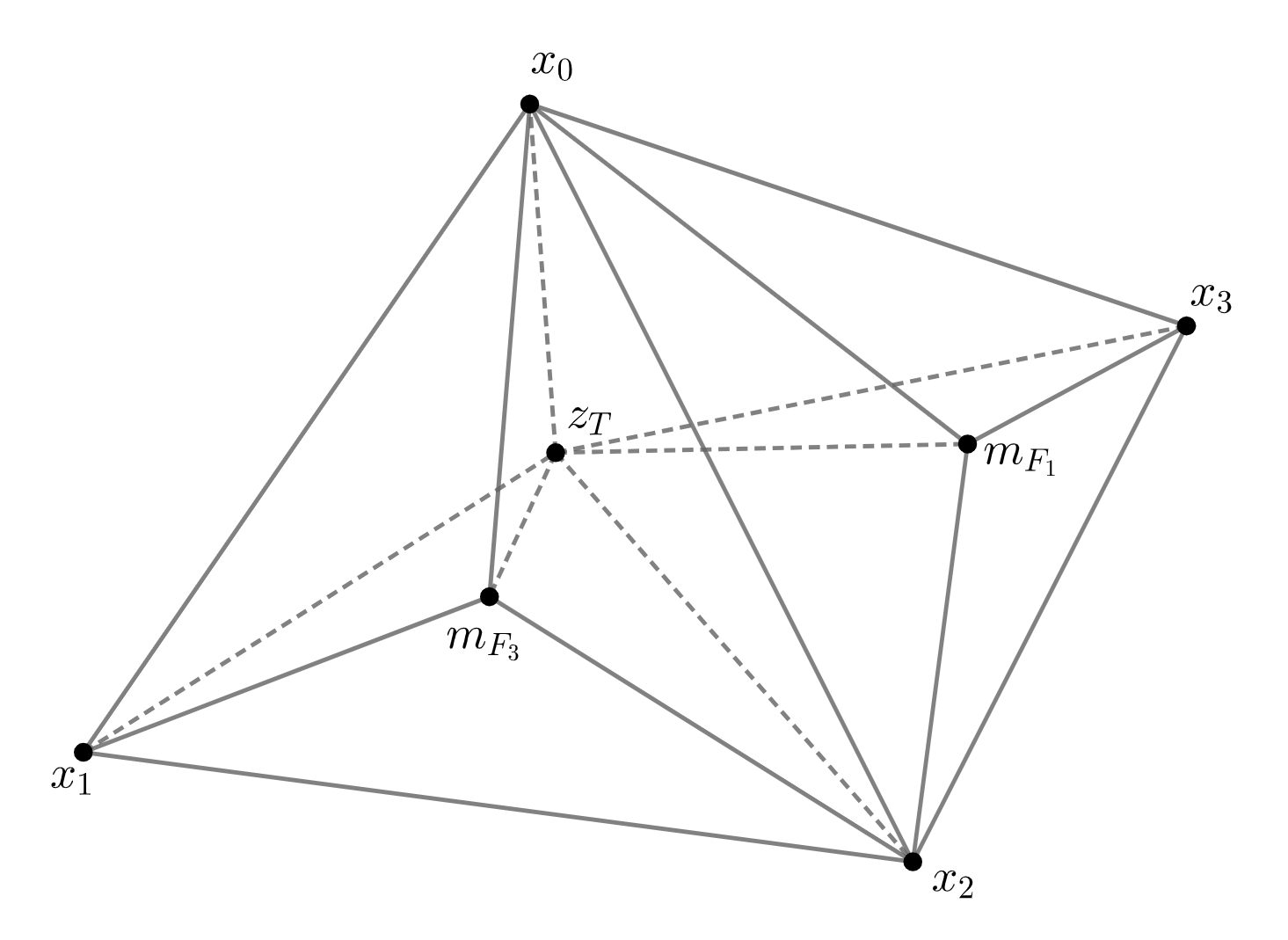
Figure 1. A representation of the Worsey-Farin split with two faces shown.

We now define local finite element spaces on each macro-tetrahedron $T\in\mathcal{T}_{h}$. To do this, we assume we have a triangulation of $T$, $T_{h}$, which could be, for example, $T_{h}=T^{\text{\rm a}}$ or $T_{h}=T^{\text{\rm wf}}$. We let $\mathcal{P}_{r}(S)$ be the space of polynomials of degree less than or equal to $r$ defined on $S$. For negative values of $r$, $\mathcal{P}_{r}(S)$ is the trivial set. We define on the triangulation $T_{h}$ of $T$ the space of discontinuous polynomials:

$$\mathcal{P}_{r}(T_{h}):=\{v\in L^{2}(T):v|_{K}\in\mathcal{P}_{r}(K),\forall K\in T_{h}\}.$$

The spaces of minimal smoothness are defined as follows.

$$V_{r}^{0}(T_{h}):= \mathcal{P}_{r}(T_{h})\cap H^{1}(T),\quad \mathring{V}_{{\color[rgb]{0,0,0}r}}^{0}(T_{h}):=\mathring{H}^{1}(T)\cap V_{{\color[rgb]{0,0,0}r}}^{0}(T_{h}),$$

$$V_{r}^{1}(T_{h}):= [\mathcal{P}_{r}(T_{h})]^{3}\cap H({\rm curl};T),\quad \mathring{V}_{{\color[rgb]{0,0,0}r}}^{1}(T_{h}):=\mathring{H}({\rm curl},T)\cap V_{{\color[rgb]{0,0,0}r}}^{1}(T_{h}),$$

$$V_{r}^{2}(T_{h}):= [\mathcal{P}_{r}(T_{h})]^{3}\cap H({\rm div};T),\quad \mathring{V}_{{\color[rgb]{0,0,0}r}}^{2}(T_{h}):=\mathring{H}({\rm div},T)\cap V_{{\color[rgb]{0,0,0}r}}^{2}(T_{h}),$$

$$V_{r}^{3}(T_{h}):= \mathcal{P}_{r}(T_{h}),\quad \mathring{V}_{{\color[rgb]{0,0,0}r}}^{2}(T_{h}):=L_{0}^{2}(T)\cap V_{{\color[rgb]{0,0,0}r}}^{2}(T_{h}),$$

where $L_{0}^{2}(T)=\{q\in L^{2}(T):\int_{T}q{\color[rgb]{0,0,0}\,dx}=0\}$. Here, we use the commonly used notation that $\mathring{(\cdot)}$ denotes the corresponding space with vanishing traces, e.g., $\mathring{H}({\rm curl},T)=\{v\in H({\rm curl},T):\ v\times n|_{{\partial}T}=0\}$ and $\mathring{H}({\rm div},T)=\{v\in H({\rm div},T):\ v\cdot n|_{{\partial}T}=0\}$. We also consider the Lagrange finite elements $\mathsf{L}_{r}^{0}(T_{h}):=V_{r}^{0}(T_{h})$ ($\mathring{\mathsf{L}}_{r}^{0}(T_{h}):=\mathring{V}^{0}(T_{h})$) , $\mathsf{L}_{r}^{i}(T_{h}):=[\mathsf{L}_{r}^{0}(T_{h})]^{3}$ ($\mathring{\mathsf{L}}_{r}^{{\color[rgb]{0,0,0}i}}(T_{h}):=[\mathring{\mathsf{L}}_{r}^{0}(T_{h})]^{3}$) for $i=1,2$ and finally $\mathsf{L}_{r}^{3}(T_{h}):=V_{r}^{0}(T_{h})$ ($\mathring{\mathsf{L}}_{r}^{3}(T_{h}):=L_{0}^{2}(T)\cap{\color[rgb]{0,0,0}\mathring{\mathsf{L}}}_{r}^{0}(T_{h})$). Finally, we define the smoother finite element spaces

$$S_{r}^{0}(T_{h}):= \{v\in\mathsf{L}_{r}^{0}(T_{h}):{\mathop{\mathrm{grad}\,}}v\in\mathsf{L}_{r-1}^{1}(T_{h})\},\quad \mathring{S}_{r}^{0}(T_{h}):=\{v\in\mathring{\mathsf{L}}_{r}^{0}(T_{h}):{\mathop{\mathrm{grad}\,}}v\in\mathring{\mathsf{L}}_{r-1}^{1}(T_{h})\},$$

$$S_{r}^{1}(T_{h}):= \{v\in\mathsf{L}_{r}^{1}(T_{h}):{\mathop{\mathrm{curl}\,}}v\in\mathsf{L}_{r-1}^{2}(T_{h})\},\quad \mathring{S}_{r}^{1}(T_{h}):=\{v\in\mathring{\mathsf{L}}_{r}^{1}(T_{h}):{\mathop{\mathrm{curl}\,}}v\in\mathring{\mathsf{L}}_{r-1}^{2}(T_{h})\},$$

$$S_{r}^{2}(T_{h}):= \{v\in\mathsf{L}_{r}^{2}(T_{h}):{\mathop{\mathrm{div}\,}}v\in\mathsf{L}_{r-1}^{3}(T_{h})\},\quad \mathring{S}_{r}^{2}(T_{h}):=\{v\in\mathring{\mathsf{L}}_{r}^{2}(T_{h}):{\mathop{\mathrm{div}\,}}v\in\mathring{\mathsf{L}}_{r-1}^{3}(T_{h})\},$$

$$S_{r}^{3}(T_{h}):= \mathsf{L}_{r}^{3}(T_{h}),\quad \mathring{S}_{r}^{3}(T_{h}):=\mathring{\mathsf{L}}_{r}^{3}(T_{h}).$$

We also define the intermediate spaces that add extra smoothness to the spaces $V_{r}^{i}(T^{\text{\rm wf}})$ on the faces of $T$.

(2.5a) $$\mathcal{V}_{r}^{2}(T^{\text{\rm wf}}) =\{v\in V_{r}^{2}(T^{\text{\rm wf}}):v\times n\text{ is continuous on each }F\in\Delta_{2}(T)\},$$

(2.5b) $$\mathring{\mathcal{V}}_{r}^{2}(T^{\text{\rm wf}}) =\{v\in\mathcal{V}_{r}^{2}(T^{\text{\rm wf}}):v\cdot n=0\text{ on each }F\in\Delta_{2}(T)\},$$

(2.5c) $$\mathcal{V}_{r}^{3}(T^{\text{\rm wf}}) =\{q\in V_{r}^{3}(T^{\text{\rm wf}}):q\text{ is continuous on each }F\in\Delta_{2}(T)\},$$

(2.5d) $$\mathring{\mathcal{V}}_{r}^{3}(T^{\text{\rm wf}}) =\mathcal{V}_{r}^{3}(T^{\text{\rm wf}})\cap L_{0}^{2}(T).$$

We see that $\mathsf{L}_{r}^{i}(T^{\text{\rm wf}})\subset\mathcal{V}_{r}^{i}(T^{\text{\rm wf}})\subset V_{r}^{i}(T^{\text{\rm wf}})$ for $i=2,3$.

3. Local Exact Sequences

One of the main results of the paper is to prove local sequences consisting of smooth piecewise polynomials are exact. The first sequences are the ones with homogeneous boundary conditions.

(3.1a) $$0\ {\xrightarrow{\hskip 14.22636pt}}\ \mathring{V}_{r}^{0}(T^{\text{\rm wf}})\ \stackrel{{\scriptstyle{\mathop{\mathrm{grad}\,}}}}{{\xrightarrow{\hskip 14.22636pt}}}\ \mathring{V}_{r-1}^{1}(T^{\text{\rm wf}})\ \stackrel{{\scriptstyle{\mathop{\mathrm{curl}\,}}}}{{\xrightarrow{\hskip 14.22636pt}}}\ \mathring{V}_{r-2}^{2}(T^{\text{\rm wf}})\ \stackrel{{\scriptstyle{\mathop{\mathrm{div}\,}}}}{{\xrightarrow{\hskip 14.22636pt}}}\ \mathring{{V}}_{r-3}^{3}(T^{\text{\rm wf}}) \xrightarrow{\hskip 14.22636pt}\ 0,$$

(3.1b) $$0\ {\xrightarrow{\hskip 14.22636pt}}\ \mathring{S}_{r}^{0}(T^{\text{\rm wf}})\ \stackrel{{\scriptstyle{\mathop{\mathrm{grad}\,}}}}{{\xrightarrow{\hskip 14.22636pt}}}\ \mathring{{\mathsf{L}}}_{r-1}^{1}(T^{\text{\rm wf}})\ \stackrel{{\scriptstyle{\mathop{\mathrm{curl}\,}}}}{{\xrightarrow{\hskip 14.22636pt}}}\ \mathring{{\mathcal{V}}}_{r-2}^{2}(T^{\text{\rm wf}})\ \stackrel{{\scriptstyle{\mathop{\mathrm{div}\,}}}}{{\xrightarrow{\hskip 14.22636pt}}}\ \mathring{{V}}_{r-3}^{3}(T^{\text{\rm wf}})\ \xrightarrow{\hskip 14.22636pt}\ 0,$$

(3.1c) $$0\ {\xrightarrow{\hskip 14.22636pt}}\ \mathring{S}_{r}^{0}(T^{\text{\rm wf}})\ \stackrel{{\scriptstyle{\mathop{\mathrm{grad}\,}}}}{{\xrightarrow{\hskip 14.22636pt}}}\ \mathring{S}_{r-1}^{1}(T^{\text{\rm wf}})\ \stackrel{{\scriptstyle{\mathop{\mathrm{curl}\,}}}}{{\xrightarrow{\hskip 14.22636pt}}}\ \mathring{\mathsf{L}}_{r-2}^{2}(T^{\text{\rm wf}})\ \stackrel{{\scriptstyle{\mathop{\mathrm{div}\,}}}}{{\xrightarrow{\hskip 14.22636pt}}}\ \mathring{\mathcal{V}}_{r-3}^{3}(T^{\text{\rm wf}})\ \xrightarrow{\hskip 14.22636pt}\ 0,$$

(3.1d) $$0\ {\xrightarrow{\hskip 14.22636pt}}\ \mathring{S}_{r}^{0}(T^{\text{\rm wf}})\ \stackrel{{\scriptstyle{\mathop{\mathrm{grad}\,}}}}{{\xrightarrow{\hskip 14.22636pt}}}\ \mathring{S}_{r-1}^{1}(T^{\text{\rm wf}})\ \stackrel{{\scriptstyle{\mathop{\mathrm{curl}\,}}}}{{\xrightarrow{\hskip 14.22636pt}}}\ \mathring{S}_{r-2}^{2}(T^{\text{\rm wf}})\ \stackrel{{\scriptstyle{\mathop{\mathrm{div}\,}}}}{{\xrightarrow{\hskip 14.22636pt}}}\ \mathring{\mathsf{L}}_{r-3}^{3}(T^{\text{\rm wf}})\ \xrightarrow{\hskip 14.22636pt}\ 0.$$

The second set of sequences does not have boundary conditions.

(3.2a) $$\mathbb{R}\ \rightarrow\ {{V}}_{r}^{0}(T^{\text{\rm wf}})\ \stackrel{{\scriptstyle{\mathop{\mathrm{grad}\,}}}}{{\xrightarrow{\hskip 14.22636pt}}}\ {{V}}_{r-1}^{1}(T^{\text{\rm wf}})\ \stackrel{{\scriptstyle{\mathop{\mathrm{curl}\,}}}}{{\xrightarrow{\hskip 14.22636pt}}}\ {{V}}_{r-2}^{2}(T^{\text{\rm wf}})\ \stackrel{{\scriptstyle{\mathop{\mathrm{div}\,}}}}{{\xrightarrow{\hskip 14.22636pt}}}\ {{V}}_{r-3}^{3}(T^{\text{\rm wf}})\ \rightarrow\ 0,$$

(3.2b) $$\mathbb{R}\ \rightarrow\ {S}_{r}^{0}(T^{\text{\rm wf}})\ \stackrel{{\scriptstyle{\mathop{\mathrm{grad}\,}}}}{{\xrightarrow{\hskip 14.22636pt}}}\ {\mathsf{L}}_{r-1}^{1}(T^{\text{\rm wf}})\ \stackrel{{\scriptstyle{\mathop{\mathrm{curl}\,}}}}{{\xrightarrow{\hskip 14.22636pt}}}\ {V}_{r-2}^{2}(T^{\text{\rm wf}})\ \stackrel{{\scriptstyle{\mathop{\mathrm{div}\,}}}}{{\xrightarrow{\hskip 14.22636pt}}}\ {V}_{r-3}^{3}(T^{\text{\rm wf}})\ \rightarrow\ 0,$$

(3.2c) $$\mathbb{R}\ \rightarrow\ {S}_{r}^{0}(T^{\text{\rm wf}})\ \stackrel{{\scriptstyle{\mathop{\mathrm{grad}\,}}}}{{\xrightarrow{\hskip 14.22636pt}}}\ {S}_{r-1}^{1}(T^{\text{\rm wf}})\ \stackrel{{\scriptstyle{\mathop{\mathrm{curl}\,}}}}{{\xrightarrow{\hskip 14.22636pt}}}\ {\mathsf{L}}_{r-2}^{2}(T^{\text{\rm wf}})\ \stackrel{{\scriptstyle{\mathop{\mathrm{div}\,}}}}{{\xrightarrow{\hskip 14.22636pt}}}\ {V}_{r-3}^{3}(T^{\text{\rm wf}})\ \rightarrow\ 0,$$

(3.2d) $$\mathbb{R}\ \rightarrow\ {S}_{r}^{0}(T^{\text{\rm wf}})\ \stackrel{{\scriptstyle{\mathop{\mathrm{grad}\,}}}}{{\xrightarrow{\hskip 14.22636pt}}}\ {S}_{r-1}^{1}(T^{\text{\rm wf}})\ \stackrel{{\scriptstyle{\mathop{\mathrm{curl}\,}}}}{{\xrightarrow{\hskip 14.22636pt}}}\ {S}_{r-2}^{2}(T^{\text{\rm wf}})\ \stackrel{{\scriptstyle{\mathop{\mathrm{div}\,}}}}{{\xrightarrow{\hskip 14.22636pt}}}\ {\mathsf{L}}_{r-3}^{3}(T^{\text{\rm wf}})\ \rightarrow\ 0.$$

The first sequences (3.1a) and (3.2a) are exact due to the results of Nédélec [14]. The major result of this section are the following theorems.

Theorem 3.1.

Let $r\geq 3$. Then the sequences (3.1) are exact.

Proof.

Again, we already know that (3.1a) is exact. The exactness of the rest of the sequences follow from the following results that are found below: Theorem 3.8, Theorem 3.14, and Theorem 3.20. ∎

Similarly, we can prove the following theorem.

Theorem 3.2.

Let $r\geq 3$. Then the sequences (3.2) are exact.

The proofs of Theorems 3.1–3.2 follow the same general procedure as [10, 7, 8]. Essentially, we build functions of the form $\mu w_{1}+\mu^{2}w_{2}+\cdots$ through an iterative procedure, where the functions $w_{j}$ are specified such that the results of Theorems 3.1–3.2 are inferred. However, due to geometric properties of the Worsey-Farin split, there are non-trivial differences between the arguments given in [10, 7, 8] and those presented here. Essentially this is due to the induced Clough-Tocher triangulation on each face $F\subset{\partial}T$, which from to the definition of $\mu$, implies that the functions $w_{j}$ are piecewise polynomials with respect to the Worsey-Farin split; in contrast, in [10, 7], the functions $w_{j}$ are simply polynomials on $T$ defined by canonical Nédélec degrees of freedom. As such, the exactness of polynomial sequences defined on (two-dimensional) Clough-Tocher triangulations plays an essential role in the proofs of Theorems 3.1–3.2.

3.1. Exact sequences on Clough–Tocher splits

Before we prove Theorems 3.1 and 3.2, we will need to use exact sequence properties of local Clough-Tocher splits. To start, we require some definitions.

Definition 3.3.

For a tetrahedron $T\in\mathcal{T}_{h}$ and face $F\in\Delta_{2}(T)$, we denote by $n_{F}:=n|_{F}$ the outward unit normal of ${\partial}T$ restricted to $F$. We let $\tau$ and $\upsilon$ be orthonormal vectors that span the tangent space of $F$. Thus, $\{\tau,\upsilon,n_{F}\}$ is an orthonormal system of $\mathbb{R}^{3}$.

Remark 3.4.

If $P(F)$ is a scalar valued space defined on $F$ then, as commonly done, and with an abuse of notation, we set $[P(F)]^{2}=\{at+b\upsilon:a,b\in P(F)\}$.

We define the Nédélec spaces on the Clough–Tocher split:

$$V_{{\rm div},r}^{1}(F^{\text{\rm ct}}):=\{v\in H({\rm div}_{F},F):v|_{Q}\in[\mathcal{P}_{r}(F)]^{2},\forall Q\in F^{\text{\rm ct}}\},\quad \mathring{V}^{1}_{{\rm div},r}(F^{\text{\rm ct}})=V_{{\rm div},r}^{1}(F^{\text{\rm ct}})\cap\mathring{H}({\rm div}_{F},F)$$

$$V_{{\rm curl},r}^{1}(F^{\text{\rm ct}}):=\{v\in H({\rm curl}_{F};,F):v|_{Q}\in[\mathcal{P}_{r}(F)]^{2},\forall Q\in F^{\text{\rm ct}}\},\quad \mathring{V}^{1}_{{\rm curl},r}(F^{\text{\rm ct}})=V_{\rm curl,r}^{1}(F^{\text{\rm ct}})\cap\mathring{H}({\rm curl}_{F},F),$$

$${V}_{r}^{2}(F^{\text{\rm ct}}):=\{v\in L^{2}(F):v|_{Q}\in\mathcal{P}_{r}(F),\forall Q\in F^{\text{\rm ct}}\},\quad \mathring{V}_{r}^{2}(F^{\text{\rm ct}}):=V_{r}^{2}(F^{\text{\rm ct}})\cap L^{2}_{0}(F),$$

and the Lagrange spaces,

$$\mathsf{L}_{r}^{0}(F^{\text{\rm ct}}):=V_{r}^{2}(F^{\text{\rm ct}})\cap H({\rm grad}_{F};F),\quad \mathring{\mathsf{L}}_{r}^{0}(F^{\text{\rm ct}}):=\mathsf{L}_{r}^{0}(F^{\text{\rm ct}})\cap\mathring{H}({\rm grad}_{F};F),$$

$$\mathsf{L}_{r}^{1}(F^{\text{\rm ct}}):=[\mathsf{L}_{r}^{0}(F^{\text{\rm ct}})]^{2},\quad \mathring{\mathsf{L}}_{r}^{1}(F^{\text{\rm ct}}):=[\mathring{\mathsf{L}}_{r}^{0}(F^{\text{\rm ct}})]^{2},$$

$$\mathsf{L}_{r}^{2}(F^{\text{\rm ct}}):=\mathsf{L}_{r}^{0}(F^{\text{\rm ct}}),\quad \mathring{\mathsf{L}}_{r}^{2}(F^{\text{\rm ct}}):=\mathring{\mathsf{L}}_{r}^{0}(F^{\text{\rm ct}})\cap L^{2}_{0}(F).$$

Finally, we define the subspaces with additional smoothness.

$$S_{r}^{0}(F^{\text{\rm ct}}):=\{v\in\mathsf{L}_{r}^{0}(F^{\text{\rm ct}}):\ {\rm grad}_{F}\,v\in{\color[rgb]{0,0,0}\mathsf{L}_{r-1}^{1}(F^{\text{\rm ct}})}\},\quad \mathring{S}_{r}^{0}(F^{\text{\rm ct}}):=\{v\in\mathring{\mathsf{L}}_{r}^{0}(F^{\text{\rm ct}}):\ {\rm grad}_{F}\,v\in{\color[rgb]{0,0,0}\mathring{\mathsf{L}}_{r-1}^{1}(F^{\text{\rm ct}})}\},$$

$$S_{{\rm div},r}^{1}(F^{\text{\rm ct}}):=\{v\in\mathsf{L}_{r}^{1}(F^{\text{\rm ct}}):\ {\rm div}_{F}\,v\in{\color[rgb]{0,0,0}\mathsf{L}_{r-1}^{2}(F^{\text{\rm ct}})}\},\quad \mathring{S}_{{\rm div},r}^{1}(F^{\text{\rm ct}}):=\{v\in\mathring{\mathsf{L}}_{r}^{1}(F^{\text{\rm ct}}):\ {\rm div}_{F}\,v\in{\color[rgb]{0,0,0}\mathring{\mathsf{L}}_{r-1}^{2}(F^{\text{\rm ct}})}\},$$

$$S_{{\rm curl},r}^{1}(F^{\text{\rm ct}}):=\{v\in\mathsf{L}_{r}^{1}(F^{\text{\rm ct}}):\ {\rm curl}_{F}\,v\in{\color[rgb]{0,0,0}\mathsf{L}_{r-1}^{2}(F^{\text{\rm ct}})}\},\quad \mathring{S}_{{\rm curl},r}^{1}(F^{\text{\rm ct}}):=\{v\in\mathring{\mathsf{L}}_{r}^{1}(F^{\text{\rm ct}}):\ {\rm curl}_{F}\,v\in{\color[rgb]{0,0,0}\mathring{\mathsf{L}}_{r-1}^{2}(F^{\text{\rm ct}})}\},$$

$$S_{r}^{2}(F^{\text{\rm ct}}):=\mathsf{L}_{r}^{2}(F^{\text{\rm ct}}),\quad \mathring{S}_{r}^{2}(F^{\text{\rm ct}}):=\mathring{\mathsf{L}}_{r}^{2}(F^{\text{\rm ct}}).$$

We note that $V_{{\rm curl},r}^{1}(F^{\text{\rm ct}})\big{(}{\color[rgb]{0,0,0}resp.,}\,S_{{\rm curl},r}^{1}(F^{\text{\rm ct}})\big{)}$ and $V_{{\rm div},r}^{1}(F^{\text{\rm ct}})\big{(}{\color[rgb]{0,0,0}resp.,}\,S_{{\rm div},r}^{1}(F^{\text{\rm ct}})\big{)}$ are isomorphic. For notational convenience we sometimes drop the ${\rm curl}$ and ${\rm div}$ from the subscripts of these spaces.

Several combinations of these spaces form exact sequences, which are summarized below.

Theorem 3.5.

Let $r\geq 1$. The following sequences are exact [1, 7].

(3.3a) $$\mathbb{R}\ {\xrightarrow{\hskip 14.22636pt}}\ {{\mathsf{L}}}_{r}^{0}(F^{\mathop{\mathrm{ct}\,}})\ \stackrel{{\scriptstyle{\rm grad}_{F}}}{{\xrightarrow{\hskip 14.22636pt}}}\ {{V}}_{{\rm curl},r-1}^{1}(F^{\mathop{\mathrm{ct}\,}})\ \stackrel{{\scriptstyle{\rm curl}_{F}}}{{\xrightarrow{\hskip 14.22636pt}}}\ {{V}}_{r-2}^{2}(F^{\mathop{\mathrm{ct}\,}})\ \xrightarrow{\hskip 14.22636pt}\ 0,$$

(3.3b) $$\mathbb{R}\ {\xrightarrow{\hskip 14.22636pt}}\ {S}_{r}^{0}(F^{\mathop{\mathrm{ct}\,}})\ \stackrel{{\scriptstyle{\rm grad}_{F}}}{{\xrightarrow{\hskip 14.22636pt}}}\ {\mathsf{L}}_{r-1}^{1}(F^{\mathop{\mathrm{ct}\,}})\ \stackrel{{\scriptstyle{\rm curl}_{F}}}{{\xrightarrow{\hskip 14.22636pt}}}\ {V}_{r-2}^{2}(F^{\mathop{\mathrm{ct}\,}})\ \xrightarrow{\hskip 14.22636pt}\ 0,$$

(3.3c) $$\mathbb{R}\ {\xrightarrow{\hskip 14.22636pt}}\ {S}_{r}^{0}(F^{\mathop{\mathrm{ct}\,}})\ \stackrel{{\scriptstyle{\rm grad}_{F}}}{{\xrightarrow{\hskip 14.22636pt}}}\ {S}_{{\color[rgb]{0,0,0}\rm curl},r-1}^{1}(F^{\mathop{\mathrm{ct}\,}})\ \stackrel{{\scriptstyle{\rm curl}_{F}}}{{\xrightarrow{\hskip 14.22636pt}}}\ {\mathsf{L}}_{r-2}^{2}(F^{\mathop{\mathrm{ct}\,}})\ \xrightarrow{\hskip 14.22636pt}\ 0,$$

(3.3d) $$0\ {\xrightarrow{\hskip 14.22636pt}}\ {\mathring{\mathsf{L}}}_{r}^{0}(F^{\mathop{\mathrm{ct}\,}})\ \stackrel{{\scriptstyle{\rm grad}_{F}}}{{\xrightarrow{\hskip 14.22636pt}}}\ {\mathring{V}}_{{\mathop{\mathrm{curl}\,}},r-1}^{1}(F^{\mathop{\mathrm{ct}\,}})\ \stackrel{{\scriptstyle{\rm curl}_{F}}}{{\xrightarrow{\hskip 14.22636pt}}}\ {\mathring{V}}_{r-2}^{2}(F^{\mathop{\mathrm{ct}\,}})\ \xrightarrow{\hskip 14.22636pt}\ 0,$$

(3.3e) $$0\ {\xrightarrow{\hskip 14.22636pt}}\ \mathring{S}_{r}^{0}(F^{\mathop{\mathrm{ct}\,}})\ \stackrel{{\scriptstyle{\rm grad}_{F}}}{{\xrightarrow{\hskip 14.22636pt}}}\ \mathring{\mathsf{L}}_{r-1}^{1}(F^{\mathop{\mathrm{ct}\,}})\ \stackrel{{\scriptstyle{\rm curl}_{F}}}{{\xrightarrow{\hskip 14.22636pt}}}\ \mathring{V}_{r-2}^{2}(F^{\mathop{\mathrm{ct}\,}})\ \xrightarrow{\hskip 14.22636pt}\ 0,$$

(3.3f) $$0\ {\xrightarrow{\hskip 14.22636pt}}\ \mathring{S}_{r}^{0}(F^{\mathop{\mathrm{ct}\,}})\ \stackrel{{\scriptstyle{\rm grad}_{F}}}{{\xrightarrow{\hskip 14.22636pt}}}\ \mathring{S}_{{\color[rgb]{0,0,0}\rm curl},r-1}^{1}(F^{\mathop{\mathrm{ct}\,}})\ \stackrel{{\scriptstyle{\rm curl}_{F}}}{{\xrightarrow{\hskip 14.22636pt}}}\ \mathring{\mathsf{L}}_{r-2}^{2}(F^{\mathop{\mathrm{ct}\,}})\ \xrightarrow{\hskip 14.22636pt}\ 0.$$

Theorems 3.5 has an alternate form that follows from a rotation of the coordinate axes, where the operators ${\rm grad}$ and ${\rm curl}$ are replaced by ${\rm rot}$ and ${\rm div}$, respectively.

Corollary 3.6.

Let $r\geq 1$. The following sequences are exact [1, 7].

(3.4a) $$\mathbb{R}\ {\xrightarrow{\hskip 14.22636pt}}\ {{\mathsf{L}}}_{r}^{0}(F^{\mathop{\mathrm{ct}\,}})\ \stackrel{{\scriptstyle{\rm rot}_{F}}}{{\xrightarrow{\hskip 14.22636pt}}}\ {{V}}_{{\rm div},r-1}^{1}(F^{\mathop{\mathrm{ct}\,}})\ \stackrel{{\scriptstyle{\rm div}_{F}}}{{\xrightarrow{\hskip 14.22636pt}}}\ {{V}}_{r-2}^{2}(F^{\mathop{\mathrm{ct}\,}})\ \xrightarrow{\hskip 14.22636pt}\ 0,$$

(3.4b) $$\mathbb{R}\ {\xrightarrow{\hskip 14.22636pt}}\ {S}_{r}^{0}(F^{\mathop{\mathrm{ct}\,}})\ \stackrel{{\scriptstyle{\rm rot}_{F}}}{{\xrightarrow{\hskip 14.22636pt}}}\ {\mathsf{L}}_{r-1}^{1}(F^{\mathop{\mathrm{ct}\,}})\ \stackrel{{\scriptstyle{\rm div}_{F}}}{{\xrightarrow{\hskip 14.22636pt}}}\ {V}_{r-2}^{2}(F^{\mathop{\mathrm{ct}\,}})\ \xrightarrow{\hskip 14.22636pt}\ 0,$$

(3.4c) $$\mathbb{R}\ {\xrightarrow{\hskip 14.22636pt}}\ {S}_{r}^{0}(F^{\mathop{\mathrm{ct}\,}})\ \stackrel{{\scriptstyle{\rm rot}_{F}}}{{\xrightarrow{\hskip 14.22636pt}}}\ {S}_{{\color[rgb]{0,0,0}\rm div},r-1}^{1}(F^{\mathop{\mathrm{ct}\,}})\ \stackrel{{\scriptstyle{\rm div}_{F}}}{{\xrightarrow{\hskip 14.22636pt}}}\ {\mathsf{L}}_{r-2}^{2}(F^{\mathop{\mathrm{ct}\,}})\ \xrightarrow{\hskip 14.22636pt}\ 0,$$

(3.4d) $$0\ {\xrightarrow{\hskip 14.22636pt}}\ {\mathring{\mathsf{L}}}_{r}^{0}(F^{\mathop{\mathrm{ct}\,}})\ \stackrel{{\scriptstyle{\rm rot}_{F}}}{{\xrightarrow{\hskip 14.22636pt}}}\ {\mathring{V}}_{{\mathop{\mathrm{div}\,}},r-1}^{1}(F^{\mathop{\mathrm{ct}\,}})\ \stackrel{{\scriptstyle{\rm div}_{F}}}{{\xrightarrow{\hskip 14.22636pt}}}\ {\mathring{V}}_{r-2}^{2}(F^{\mathop{\mathrm{ct}\,}})\ \xrightarrow{\hskip 14.22636pt}\ 0,$$

(3.4e) $$0\ {\xrightarrow{\hskip 14.22636pt}}\ \mathring{S}_{r}^{0}(F^{\mathop{\mathrm{ct}\,}})\ \stackrel{{\scriptstyle{\rm rot}_{F}}}{{\xrightarrow{\hskip 14.22636pt}}}\ \mathring{\mathsf{L}}_{r-1}^{1}(F^{\mathop{\mathrm{ct}\,}})\ \stackrel{{\scriptstyle{\rm div}_{F}}}{{\xrightarrow{\hskip 14.22636pt}}}\ \mathring{V}_{r-2}^{2}(F^{\mathop{\mathrm{ct}\,}})\ \xrightarrow{\hskip 14.22636pt}\ 0,$$

(3.4f) $$0\ {\xrightarrow{\hskip 14.22636pt}}\ \mathring{S}_{r}^{0}(F^{\mathop{\mathrm{ct}\,}})\ \stackrel{{\scriptstyle{\rm rot}_{F}}}{{\xrightarrow{\hskip 14.22636pt}}}\ \mathring{S}_{{\color[rgb]{0,0,0}\rm div},r-1}^{1}(F^{\mathop{\mathrm{ct}\,}})\ \stackrel{{\scriptstyle{\rm div}_{F}}}{{\xrightarrow{\hskip 14.22636pt}}}\ \mathring{\mathsf{L}}_{r-2}^{2}(F^{\mathop{\mathrm{ct}\,}})\ \xrightarrow{\hskip 14.22636pt}\ 0.$$

Remark 3.7.

From Theorem 3.5, Corollary 3.6, the well-known dimension formulas of the Nédélec and Lagrange spaces, and the rank–nullity theorem, one easily finds the dimensions of the smoother spaces $S^{k}_{r}(F^{\text{\rm ct}})$ (cf. [7]). These counts are summarized in Table 1.

Table 1. Dimension counts of the canonical (two–dimensional) Nédélec, Lagrange, and smooth spaces with and without boundary conditions with respect to the Clough–Tocher split. Here, $\dim V_{{\rm div},r}^{1}(F^{\text{\rm ct}})=\dim V_{{\rm curl},r}^{1}(F^{\text{\rm ct}})=:\dim V_{r}^{1}(F^{\text{\rm ct}})$

	$k=0$	$k=1$	$k=2$
$\dim V_{r}^{k}(F^{\text{\rm ct}})$	$\frac{1}{2}(3r^{2}+3r+2)$	$3(r+1)^{2}$	$\frac{3}{2}(r+1)(r+2)$
$\dim\mathring{V}_{r}^{k}(F^{\text{\rm ct}})$	$\frac{1}{2}(3r^{2}-3r+2)$	$3r(r+1)$	$\frac{3}{2}(r+1)(r+2)-1$
$\dim\mathsf{L}_{r}^{k}(F^{\text{\rm ct}})$	$\frac{1}{2}(3r^{2}+3r+2)$	$3r^{2}+3r+2$	$\frac{1}{2}(3r^{2}+3r+2)$
$\dim\mathring{\mathsf{L}}_{r}^{k}(F^{\text{\rm ct}})$	$\frac{1}{2}(3r^{2}-3r+2)$	$3r^{2}-3r+2$	$\frac{3}{2}r(r-1)$
$\dim S_{r}^{k}(F^{\text{\rm ct}})$	$\frac{3}{2}(r^{2}-r+2)$	$3r^{2}+3$	$\frac{1}{2}(3r^{2}+3r+2)$
$\dim\mathring{S}_{r}^{k}(F^{\text{\rm ct}})$	$\frac{3}{2}(r^{2}-5r+6)$	$3r^{2}-9r+6$	$\frac{3}{2}r(r-1)$
$\dim\mathcal{R}_{r}^{k}(F^{\text{\rm ct}})$	$\frac{3}{2}(r-1)(r-2)$	$3(r-1)^{2}$	—

We will use the following intermediate spaces when developing commuting projections on the Worsey-Farin split:

$$\mathcal{R}_{r}^{0}(F^{\mathop{\mathrm{ct}\,}}):=\{v\in S_{r}^{0}(F^{\mathop{\mathrm{ct}\,}}):v|_{\partial F}=0\},\quad\mathcal{R}_{r}^{1}(F^{\mathop{\mathrm{ct}\,}}):=\{v\in S_{{\mathop{\mathrm{div}\,}},r}^{1}(F^{\mathop{\mathrm{ct}\,}}):v|_{\partial F}=0\}.$$

It is shown in [13] that $\dim\mathcal{R}_{r}^{0}(F^{\mathop{\mathrm{ct}\,}})=\frac{3}{2}(r-1)(r-2)$ and $\dim\mathcal{R}_{r}^{1}(F^{\mathop{\mathrm{ct}\,}})=3(r-1)^{2}.$

3.2. Surjectivity of the divergence operator on discrete local spaces

The goal of this section is to prove the following theorem.

Theorem 3.8.

Let $r\geq 0$. Then:

1. for each $p\in\mathring{\mathcal{V}}_{r}^{3}(T^{\text{\rm wf}})$, there exists a $v\in\mathring{\mathsf{L}}_{r+1}^{2}(T^{\text{\rm wf}})$ such that ${\mathop{\mathrm{div}\,}}v=p$.

2. for each $p\in\mathring{V}_{r}^{3}(T^{\text{\rm wf}})$, there exists a $v\in\mathsf{L}_{r+1}^{2}(T^{\text{\rm wf}})\cap\mathring{V}_{r+1}^{2}(T^{\text{\rm wf}})$ such that ${\mathop{\mathrm{div}\,}}v=p$.

3. for each $p\in V_{r}^{3}(T^{\text{\rm wf}})$, there exists a $v\in\mathsf{L}_{r+1}^{2}(T^{\text{\rm wf}})$ such that ${\mathop{\mathrm{div}\,}}v=p$.

4. for each $p\in\mathring{\mathsf{L}}_{r}^{3}(T^{\text{\rm wf}})$ (resp., $p\in\mathsf{L}_{r}^{3}(T^{\text{\rm wf}})$), there exists a $v\in\mathring{S}_{r+1}^{2}(T^{\text{\rm wf}})$ (resp., $v\in S_{r+1}^{2}(T^{\text{\rm wf}})$) such that ${\mathop{\mathrm{div}\,}}v=p$.

The proofs of Theorem 3.8 parts (i) and (ii) depends on five preliminary lemmas.

Lemma 3.9.

Let $r\geq 1$ and $s\geq 0$ be integers. Then for any $q\in\mathcal{V}_{r}^{3}(T^{\text{\rm wf}})$, there exists $w\in\mathsf{L}_{r}^{2}(T^{\text{\rm wf}})$ and $g\in V_{r-1}^{3}(T^{\text{\rm wf}})$, such that $\mu^{s}q={\mathop{\mathrm{div}\,}}(\mu^{s+1}w)+\mu^{s+1}g$.

Proof.

Let $q\in\mathcal{V}_{r}^{3}(T^{\text{\rm wf}})$ and $s\geq 0$. Because $q|_{F_{i}}$ is continuous on each $F_{i}\in\Delta_{2}(T)$, there exists $b_{i}\in\mathcal{P}_{r}(F_{i})$ such that $b_{i}=q|_{F_{i}}$ on ${\partial}F_{i}$. Thus $q-b_{i}$ is continuous on $F_{i}$ and vanishes on $\partial F_{i}$. Consequently, there exists $a_{i}\in\mathsf{L}_{r}^{{\color[rgb]{0,0,0}3}}(T^{\text{\rm wf}})$ such that $a_{i}=(q-b_{i})$ on $F_{i}$ and $\text{supp}(a_{i})\subseteq K_{i}$. Using the divergence-conforming Nédélec degrees of freedom of the second kind [14] , and the fact that ${\mathop{\mathrm{grad}\,}}\mu_{i}$ is parallel to the outward unit normal of $F_{i}$, there exists $w_{1}\in[\mathcal{P}_{r}(T)]^{3}$ such that

$$(s+1)w_{1}\cdot{\mathop{\mathrm{grad}\,}}\mu_{i}=b_{i}\quad\text{on }F_{i}.$$

We also define $w_{2}\in\mathsf{L}_{r}^{2}(T^{\text{\rm wf}})$ as

$$w_{2}:=\frac{1}{s+1}\sum_{i=1}^{4}a_{i}\ell_{i},$$

where $\ell_{i}:=\frac{{\mathop{\mathrm{grad}\,}}\mu_{i}}{|{\mathop{\mathrm{grad}\,}}\mu_{i}|^{2}}$. Finally, we set $w:=w_{1}+w_{2}\in\mathsf{L}_{r}^{2}(T^{\text{\rm wf}})$. We then see that

$$q-(s+1)w\cdot{\mathop{\mathrm{grad}\,}}\mu=0\quad\text{ on }\partial T,$$

and, hence, there exists $p\in V_{r-1}^{3}(T^{\text{\rm wf}})$ such that

$$q=(s+1)w\cdot{\mathop{\mathrm{grad}\,}}\mu+\mu p\quad\text{ on }T.$$

Setting $g:={\color[rgb]{0,0,0}p-{\mathop{\mathrm{div}\,}}w}\in V_{r-1}^{3}(T^{\text{\rm wf}})$ we have

$$\mu^{s}q= (s+1)\mu^{s}w\cdot{\mathop{\mathrm{grad}\,}}\mu+\mu^{s+1}p={\mathop{\mathrm{div}\,}}(\mu^{{\color[rgb]{0,0,0}s+1}}w)+\mu^{s+1}g.$$

∎

Lemma 3.10.

Let $K\in T^{\text{\rm a}}$, $F\in\Delta_{2}(T)$ with $F\subset\partial K$ and let $n_{F}$ denote the outward pointing unit normal to $F$. If $p\in\mathring{\mathsf{L}}_{r}^{1}(F^{\text{\rm ct}})$ then there exists $q\in\mathsf{L}_{r}^{1}(T^{\text{\rm wf}})$ such that $q|_{F}=p$, $\text{supp}(q)\subset K$ and $q\cdot{\color[rgb]{0,0,0}n_{F}}=0$ on $K$.

Proof.

Let $\{\tau,\upsilon,n_{F}\}$ be an orthonormal set with $\tau$ and $\upsilon$ parallel to $F$. Then $p=a\tau+b\upsilon$ for some $a,b\in\mathring{\mathsf{L}}_{r}^{0}(F^{\text{\rm ct}})$. We extend $a$ and $b$ to all of $K$, which we denote by $\tilde{a},\tilde{b}\in{\color[rgb]{0,0,0}\mathsf{L}}_{r}^{0}(K^{\text{\rm wf}})$, by setting all the other Lagrange degrees of freedom to be zero. In particular $\tilde{a}$ and $\tilde{b}$ vanish on $\partial K\backslash F$. Hence, we can further extend them by zero to all of $T$ to obtain $\tilde{a},\tilde{b}\in{\color[rgb]{0,0,0}\mathsf{L}}_{r}^{0}(T^{\text{\rm wf}})$. We then set $q=\tilde{a}\tau+\tilde{b}\upsilon$. ∎

Lemma 3.11.

For any $\theta\in V_{r}^{3}(T^{\text{\rm wf}})$, with $r\geq 0$, there exists $\psi\in\mathsf{L}_{r+1}^{2}(T^{\text{\rm wf}})\cap\mathring{V}_{r+1}^{2}(T^{\text{\rm wf}})$ and $\gamma\in\mathcal{V}_{r}^{3}(T^{\text{\rm wf}})$ such that

(3.5) $$\mu^{s}\theta ={\mathop{\mathrm{div}\,}}(\mu^{s}\psi)+\mu^{s}\gamma\qquad\forall s\geq 0.$$

Proof.

Let $K_{i}\in{\color[rgb]{0,0,0}T^{\text{\rm a}}}$ be the tetrahedron containing the face $F_{i}\in\Delta_{2}(T)$, and let $\kappa_{i}\in V_{0}^{3}(T^{\text{\rm a}})\subset V_{0}^{3}(T^{\text{\rm wf}})$ be defined on $K_{i}$ as $\kappa_{i}=\frac{1}{|F_{i}|}\int_{F_{i}}\theta{\color[rgb]{0,0,0}\,dA}$. Then on $F_{i}$,

$$\int_{F_{i}}(\theta-\kappa_{i}){\color[rgb]{0,0,0}\,dA}=0,$$

so $(\theta-\kappa_{i})_{F_{i}}\in\mathring{V}_{r}^{2}(F^{\text{\rm ct}}_{i})$ by definition. Hence, by Corollary 3.6, there exists a function $\rho_{i}\in\mathring{\mathsf{L}}_{r+1}^{1}(F^{\text{\rm ct}}_{i})$ such that

(3.6) $${\rm div}_{F_{i}}\,\rho_{i}=(\theta-\kappa_{i})\quad\text{ on }{F_{i}}.$$

By Lemma 3.10, there exists an extension $\psi_{i}\in\mathsf{L}_{r+1}^{{2}}(T^{\text{\rm wf}})$ such that $\psi_{i}{\color[rgb]{0,0,0}|_{F_{i}}}=\rho_{i}$, $\text{supp}(\psi_{i})\subseteq K_{i}$, and $\psi_{i}\cdot n_{F_{i}}=0$ on $K_{i}$. We then define $\psi=\sum_{i=0}^{3}\psi_{i}\in\mathsf{L}_{r+1}^{{2}}(T^{\text{\rm wf}})\cap\mathring{V}_{r+1}^{2}(T^{\text{\rm wf}})$. The construction of $\psi$, and using (2.2), yields the identities

(3.7) $$\psi\cdot n_{F_{i}}= 0\qquad \text{on }K_{i},$$

(3.8) $${\mathop{\mathrm{div}\,}}\psi= {\rm div}_{F_{i}}\,\rho_{i}\qquad {\text{on }F_{i}}.$$

Now set $\gamma:=\theta-{\mathop{\mathrm{div}\,}}\psi$, so that $\gamma=\kappa_{i}$ on $F_{i}$ by (3.8) and (3.6). Since $\kappa_{i}$ is continuous on $F_{i}$, it follows that $\gamma\in\mathcal{V}_{r}^{3}(T^{\text{\rm wf}})$. Rearranging terms yields $\theta={\mathop{\mathrm{div}\,}}\psi+\gamma$, which proves the result in the case $s=0$. Furthermore, since ${\mathop{\mathrm{grad}\,}}\mu$ is parallel to $n_{F_{i}}$ on each $K_{i}$, we have by (3.7),

$$\mu^{s}\theta-{\mathop{\mathrm{div}\,}}(\mu^{s}\psi) =\mu^{s}\theta-\mu^{s}{\mathop{\mathrm{div}\,}}\psi-s\mu^{s-1}\psi\cdot{\mathop{\mathrm{grad}\,}}\mu=\mu^{s}\gamma,$$

which is the desired result. ∎

Lemma 3.12.

Let $q\in\mathcal{V}_{r}^{3}(T^{\text{\rm wf}})$ with $r\geq 1$, and $s\geq 0$. Then there exists $v\in\mathsf{L}_{r}^{2}(T^{\text{\rm wf}})$ and $p\in\mathcal{V}_{r-1}^{3}(T^{\text{\rm wf}})$ such that $\mu^{s}q={\mathop{\mathrm{div}\,}}(\mu^{s+1}v)+\mu^{s+1}p$.

Proof.

By Lemma 3.9, there exist $w\in\mathsf{L}_{r}^{2}(T^{\text{\rm wf}})$ and $g\in V_{r-1}^{3}(T^{\text{\rm wf}})$ such that

$$\mu^{s}q ={\mathop{\mathrm{div}\,}}(\mu^{s+1}w)+\mu^{s+1}g.$$

Since $g\in V_{r-1}^{3}(T^{\text{\rm wf}})$, Lemma 3.11 yields the existence of $\psi\in\mathsf{L}_{r}^{2}(T^{\text{\rm wf}})$ and $p\in\mathcal{V}_{r-1}^{3}(T^{\text{\rm wf}})$ such that

$$\mu^{s+1}g={\mathop{\mathrm{div}\,}}(\mu^{s+1}\psi)+\mu^{s+1}p.$$

Therefore, $\mu^{s}q={\mathop{\mathrm{div}\,}}(\mu^{s+1}(w+\psi))+\mu^{s+1}p$. Setting $v=w+\psi$ achieves the desired result. ∎

The final preliminary lemma follows from a result shown in [7].

Lemma 3.13.

Let $s\geq 0$, and let $q\in\mathcal{V}_{0}^{3}(T^{\text{\rm wf}})$ with $\int_{T}\mu^{s}q{\color[rgb]{0,0,0}\,dx}=0$. Then there exists $w\in\mathsf{L}_{0}^{2}(T^{\text{\rm wf}})$ such that $\mu^{s}q={\mathop{\mathrm{div}\,}}(\mu^{s+1}w)$.

Proof.

Since $q\in\mathcal{V}_{0}^{3}(T^{\text{\rm wf}})$ it is easy to see that $q\in V_{0}^{3}(T^{\text{\rm a}})$. From [7, Lemma 3.11], there exists $w\in[\mathcal{P}_{0}(T)]^{3}\subset\mathsf{L}_{0}^{2}(T^{\text{\rm wf}})$ such that ${\mathop{\mathrm{div}\,}}(\mu^{s+1}w)={\color[rgb]{0,0,0}\mu^{s}}q$. ∎

We can now prove Theorem 3.8 parts (i) and (ii).

Proof of Theorem 3.8, part (i).

The case $r=0$ follows immediately from Lemma 3.13 with $s=0$. Now consider the case $r\geq 1$. Let $0\leq j\leq r-1$ and assume that we have found $w_{r},w_{r-1},\ldots,w_{r-j}$ with $w_{\ell}\in\mathsf{L}_{\ell}^{2}(T^{\text{\rm wf}})$ and $p_{r-j}\in\mathcal{V}_{r-j}^{3}(T^{\text{\rm wf}})$ such that

$$p= {\mathop{\mathrm{div}\,}}(\mu w_{r}+\mu^{2}w_{r-1}+\cdots+\mu^{j+1}w_{r-j})+\mu^{j+1}p_{r-(j+1)}.$$

If $0\leq j<r-1$ then we apply Lemma 3.12 to find $w_{r-(j+1)}\in\mathsf{L}_{r-(j+1)}^{2}(T^{\text{\rm wf}})$ and $p_{r-(j+2)}\in{\mathcal{V}_{r-(j+2)}^{3}(T^{\text{\rm wf}})}$ such that

$$\mu^{j+1}p_{r-(j+1)}={\mathop{\mathrm{div}\,}}(\mu^{j+2}w_{r-(j+1)})+\mu^{j+2}p_{r-(j+2)}.$$

In which case we obtain

$$p= {\mathop{\mathrm{div}\,}}(\mu w_{r}+\mu^{2}w_{r-1}+\cdots+\mu^{j+2}w_{r-(j+1)})+\mu^{j+2}p_{r-(j+2)}.$$

After taking care of the base case $j=0$, and continuining by induction we arrive at

$$p={\mathop{\mathrm{div}\,}}(\mu w_{r}+\mu^{2}w_{r-1}+\cdots+\mu^{r}w_{1})+\mu^{r}p_{0}.$$

By the hypothesis $\int_{T}p{\color[rgb]{0,0,0}\,dx}=0$, there holds $\int_{T}\mu^{r}p_{0}{\color[rgb]{0,0,0}\,dx}=0$. By Lemma 3.13, there exists $w_{0}\in\mathsf{L}_{0}^{2}(T^{\text{\rm wf}})$ such that ${\mathop{\mathrm{div}\,}}(\mu^{r+1}w_{0})=\mu^{r}p_{0}$. The result follows by setting $v=\mu w_{r}+\mu^{2}w_{r-1}+\cdots+\mu^{r}w_{1}+\mu^{r+1}w_{0}$.

∎

Proof of Theorem 3.8, part (ii).

By Lemma 3.11 (with $s=0$), there exists $\psi\in\mathsf{L}_{r+1}^{2}(T^{\text{\rm wf}})\cap\mathring{V}_{r+1}^{2}(T^{\text{\rm wf}})$ and $\gamma\in\mathcal{V}_{r}^{3}(T^{\text{\rm wf}})$ satisfying

$$p={\mathop{\mathrm{div}\,}}\psi+\gamma.$$

Note that $\int_{T}p{\color[rgb]{0,0,0}\,dx}=0$, and $\int_{T}{\mathop{\mathrm{div}\,}}\psi\,dx=\int_{\partial T}\psi\cdot n\,dA=0$ since $\psi\cdot n=0$ on $\partial T$. Thus, we have that $\int_{T}\gamma{\color[rgb]{0,0,0}\,dx}=0$ which implies $\gamma\in\mathring{\mathcal{V}}_{r}^{3}(T^{\text{\rm wf}})$. Therefore, we apply part (i) of Theorem 3.8 to find $g\in\mathring{\mathsf{L}}_{r+1}(T^{\text{\rm wf}})$ such that ${\mathop{\mathrm{div}\,}}g=\gamma$. The result follows by setting $v=\psi+g$. ∎

We now prove parts (iii) and (iv) of Theorem 3.8, which are corollaries to parts (i) and (ii).

Proof of Theorem 3.8, part (iii).

We decompose $p=(p-\overline{p})+\overline{p}$ where $\overline{p}:=\frac{1}{|T|}\int_{T}p{\color[rgb]{0,0,0}\,dx}$. There exists $w\in[\mathcal{P}_{1}(T)]^{3}$ such that ${\mathop{\mathrm{div}\,}}w=\overline{p}$, and by part (ii) of Theorem 3.8 we have $\psi\in\mathsf{L}_{r+1}^{2}(T^{\text{\rm wf}})\cap\mathring{V}_{r+1}^{2}(T^{\text{\rm wf}})$ such that ${\mathop{\mathrm{div}\,}}\psi=p-\overline{p}$. Thus, setting $v:=\psi+w$ completes the proof. ∎

Proof of Theorem 3.8, part (iv).

Let $p\in{\mathring{\mathsf{L}}_{r}^{3}(T^{\text{\rm wf}})}\subset\mathring{\mathcal{V}}_{r}^{3}(T^{\text{\rm wf}})$. Applying part (i) of Theorem 3.8, we find $v\in{\mathring{\mathsf{L}}_{r+1}^{2}(T^{\text{\rm wf}})}$ such that ${\mathop{\mathrm{div}\,}}v=p$. But clearly $v\in\mathring{S}_{r+1}^{2}(T^{\text{\rm wf}})$, since ${\mathop{\mathrm{div}\,}}v$ belongs to $\mathring{\mathsf{L}}_{r}^{3}(T^{\text{\rm wf}})$. ∎

3.3. Surjectivity of the curl operator on discrete local spaces

The main goal of this section is to derive the analagous results of Section 3.2, but for the curl operator; that is, we show that the curl operator acting on piecewise polynomial spaces with respect to the Worsey–Farin split is surjective onto spaces of divergence–free functions. The main result of this section is the following.

Theorem 3.14.

Let $r\geq 0$. Then:

1. for any $v\in\mathring{\mathcal{V}}_{r}^{2}(T^{\text{\rm wf}})$ satisfying ${\mathop{\mathrm{div}\,}}v=0$ there exists $w\in\mathring{\mathsf{L}}_{r+1}^{1}(T^{\text{\rm wf}})$ satisfying ${\mathop{\mathrm{curl}\,}}w=v$.

2. let $v\in V_{r}^{2}(T^{\text{\rm wf}})$ with ${\mathop{\mathrm{div}\,}}v=0$. Then there exists $w\in{\mathsf{L}_{r+1}^{1}(T^{\text{\rm wf}})}$ such that ${\mathop{\mathrm{curl}\,}}w=v$.

3. for each $v\in{\mathring{\mathsf{L}}_{r}^{2}(T^{\text{\rm wf}})}$ (resp., $v\in{\mathsf{L}_{r}^{2}(T^{\text{\rm wf}})}$) with ${\mathop{\mathrm{div}\,}}v=0$, there exists a $w\in\mathring{S}_{r+1}^{1}(T^{\text{\rm wf}})$ (resp., $w\in S_{r+1}^{1}(T^{\text{\rm wf}})$) such that ${\mathop{\mathrm{curl}\,}}w=v$.

4. for each $v\in\mathring{S}_{r}^{2}(T^{\text{\rm wf}})$ (resp., $v\in S_{r}^{2}(T^{\text{\rm wf}})$) with ${\mathop{\mathrm{div}\,}}v=0$, there exists $w\in\mathring{S}_{r+1}^{1}(T^{\text{\rm wf}})$ (resp., $w\in S_{r+1}^{1}(T^{\text{\rm wf}})$) such that ${\mathop{\mathrm{curl}\,}}w=v$.

We omit the proofs of parts (iii) and (iv) of Theorem 3.14 since they easily follow from parts (i) and (ii) of the same theorem.

Before we prove parts (i) and (ii) of Theorem 3.14, we first establish several lemmas.

Lemma 3.15.

Let $r\geq 0$ and let $v\in\mathring{\mathcal{V}}_{r}^{2}(T^{\text{\rm wf}})$. Then there exist functions $z\in[\mathcal{P}_{r}(T^{\text{\rm wf}})]^{3}$ and $\gamma\in[\mathcal{P}_{r-1}(T^{\text{\rm wf}})]^{3}$ such that

(3.9) $$v={\mathop{\mathrm{grad}\,}}\mu\times z+\mu\gamma,$$

and so ${\mathop{\mathrm{grad}\,}}\mu\times z$ is continuous on $F$ for each $F\in\Delta_{2}(T)$. Moreover, for each $e\in\Delta_{1}(T)$ and its unit tangent vector $t$, $z\cdot t$ is single-valued on $e$.

Proof.

By [7, Lemma 4.1], there exists $z\in[\mathcal{P}_{r}(T^{\text{\rm wf}})]^{3}$ and $\gamma\in[\mathcal{P}_{r-1}(T^{\text{\rm wf}})]^{3}$ such that (3.9) holds. For each $F\in\Delta_{2}(T)$, there holds $v={\mathop{\mathrm{grad}\,}}\mu\times z$ on $F$, and hence ${\mathop{\mathrm{grad}\,}}\mu\times z$ is continuous on $F$. Following exactly the proof of [7, Lemma 4.2], we see that $z\cdot t$ is single-valued for all $e\in\Delta_{1}(T)$. ∎

Lemma 3.16.

For any $v\in\mathring{\mathcal{V}}_{r}^{2}(T^{\text{\rm wf}})$, with $r\geq 1$, and any integer $s\geq 0$, there exists $w\in\mathsf{L}_{r}^{1}(T^{\text{\rm wf}})$ and $g\in V_{r-1}^{2}(T^{\text{\rm wf}})$ such that

(3.10) $$\mu^{s}v ={\mathop{\mathrm{curl}\,}}(\mu^{s+1}w)+\mu^{s+1}g.$$

Proof.

From Lemma 3.15, there exists $z\in[\mathcal{P}_{r}(T^{\text{\rm wf}})]^{3}$ and $\gamma\in[\mathcal{P}_{r-1}(T^{\text{\rm wf}})]^{3}$ satisfying (3.9) with $z\times{\mathop{\mathrm{grad}\,}}\mu$ continuous on $F$ for each $F\in\Delta_{2}(T)$ and $z\cdot t$ is single-valued for all $e\in\Delta_{1}(T)$. Let $\{F_{i}\}_{i=0}^{3}$ be the four faces of $T$. For each $i$ we choose $b_{i}\in[\mathcal{P}_{r}(F_{i})]^{2}$ so that $b_{i}={z_{F_{i}}}$ on $\partial F_{i}$, which we are allowed to do since $z\times{\mathop{\mathrm{grad}\,}}\mu$ is continuous on $F_{i}$. Since $z\cdot t$ is single-valued for all $e\in\Delta_{1}(T)$, we have that $b_{i}\cdot t|_{e}=b_{j}\cdot t|_{e}$ if $e=F_{i}\cap F_{j}$. Hence, using the curl-conforming Nédélec degrees of freedom of the second kind [14], there exists $w_{1}\in[\mathcal{P}_{r}(T)]^{3}$ such that ${(w_{1})_{F_{i}}}=b_{i}\text{ on }F_{i}\text{ for }0\leq i\leq 3.$

Since ${z_{F_{i}}-b_{i}}\in\mathring{\mathsf{L}}_{r}^{1}(F^{\text{\rm ct}}_{i})$, according to Lemma 3.10, there exists $a_{i}\in\mathsf{L}_{r}^{1}(T^{\text{\rm wf}})$ such that $\text{supp }(a_{i})\subset K_{i}$ and ${(a_{i})_{F_{i}}}={z_{F_{i}}-b_{i}}$ on $F_{i}$. We set $w_{2}:=\sum_{i=0}^{3}a_{i}$ and finally $w:=\frac{1}{s+1}(w_{1}+w_{2})\in{\mathsf{L}_{r}^{1}(T^{\text{\rm wf}})}$. Hence,

$$(s+1){w_{F_{i}}}={(w_{1})_{F_{i}}+(w_{2})_{F_{i}}}={b_{i}+(a_{i})_{F_{i}}}=z_{F_{i}}.$$

From this we deduce $(s+1){\mathop{\mathrm{grad}\,}}\mu\times w={\mathop{\mathrm{grad}\,}}\mu\times z$ on each $F_{i}$.

Thus, there exists $\phi\in[\mathcal{P}_{r-1}(T^{\text{\rm wf}})]^{3}$ such that

(3.11) $$(s+1){\mathop{\mathrm{grad}\,}}\mu\times w={\mathop{\mathrm{grad}\,}}\mu\times z+\mu\phi=v+\mu({\phi}-\gamma)\quad\text{ on }T.$$

We write ${\mathop{\mathrm{curl}\,}}(\mu^{s+1}w)=(s+1)\mu^{s}{\mathop{\mathrm{grad}\,}}\mu\times w+\mu^{s+1}{\mathop{\mathrm{curl}\,}}w=\mu^{s}v+\mu^{s+1}({\mathop{\mathrm{curl}\,}}w-\gamma+\phi)$. Setting $g:=-({\mathop{\mathrm{curl}\,}}w-\gamma+\phi)$, we have that (3.10) holds. Finally, since $\mu^{s}v\cdot n$ and ${\mathop{\mathrm{curl}\,}}(\mu^{s+1}w)\cdot n$ are single-valued on interior faces, $\mu^{s+1}g\cdot n$ is single-valued. Because $\mu$ is continuous and strictly positive in the interior of $T$, this implies $g\cdot n$ is single-valued on interior faces, and thus $g\in V_{r-1}^{2}(T^{\text{\rm wf}})$. ∎

Lemma 3.17.

Let $r\geq 0$ and $s\geq 0$ be integers. For any $g\in\mathring{V}_{r}^{2}(T^{\text{\rm wf}})$ there exists $\psi\in\mathsf{L}_{r+1}^{1}(T^{\text{\rm wf}})$ and $\gamma\in\mathring{\mathcal{V}}_{r}^{2}(T^{\text{\rm wf}})$ such that

$$\mu^{s}g ={\mathop{\mathrm{curl}\,}}(\mu^{s}\psi)+\mu^{s}\gamma.$$

Proof.

Let $\{F_{i}\}_{i=0}^{3}$ be the four faces of $T$ so that $g_{F_{i}}\in H({\rm div}_{F_{i}};F_{i})$ by Lemma B.1. We use the (two-dimensional) divergence-conforming Nédélec degrees of freedom to construct $p_{i}\in[\mathcal{P}_{r}(F_{i})]^{2}$ so that for $r\geq 1$,

$$p_{i}\cdot(n_{F}\times t)=g_{F_{i}}\cdot(n_{F}\times t)\qquad\text{ on }e,\forall e\in\Delta_{1}(F_{i}),$$

where $t$ is the unit vector tangent to the edge $e$. If $r=0$, we can satisfy the above equation for two of the three edges, however, on the third edge the equation will be automatically satisfied since ${\rm div}_{F_{i}}\,(g_{F_{i}}-p_{i})=0$.

Using $g_{F_{i}}-p_{i}\in\mathring{V}_{{\rm div},r}^{1}(F^{\text{\rm ct}}_{i})$ we have that ${\mathop{\mathrm{div}\,}}(g_{F_{i}}-p_{i})\in\mathring{V}_{r-1}^{2}(F^{\text{\rm ct}}_{i})$. By Corollary 3.6, there exists $m_{i}\in\mathring{\mathsf{L}}_{r}^{1}(F^{\text{\rm ct}}_{i})$ so that ${\rm div}_{F_{i}}\,m_{i}={\rm div}_{F_{i}}\,(g_{F_{i}}-p_{i})$ on $F_{i}$. Thus, if we let $\theta_{i}:=p_{i}+m_{i}$ we have $\theta_{i}\in\mathsf{L}_{r}^{1}(F^{\text{\rm ct}}_{i})$ and $g_{F_{i}}-\theta_{i}\in\mathring{V}_{{\rm div},r}^{1}(F^{\text{\rm ct}}_{i})$ with ${\rm div}_{F_{i}}\,(g_{F_{i}}-\theta_{i})=0$. By Corollary 3.6, there exists $\kappa_{i}\in\mathring{\mathsf{L}}_{r+1}^{0}(F^{\text{\rm ct}}_{i})$ such that $\text{rot}_{F_{i}}\kappa_{i}=g_{F_{i}}-\theta_{i}$. Since $\kappa_{i}$ vanishes on $\partial F_{i}$ there exists $\beta_{i}\in\mathring{\mathsf{L}}_{r+1}^{0}(T^{\text{\rm wf}})$ with $\text{supp }(\beta_{i})\subset K_{i}$ such that $\beta_{i}=\kappa_{i}$ on $F_{i}$. We let $\psi=\sum_{i=0}^{3}\beta_{i}n_{F_{i}}\in\mathring{\mathsf{L}}_{r+1}^{1}(T^{\text{\rm wf}})$. Note that this immediately implies that ${\mathop{\mathrm{grad}\,}}\mu\times\psi\equiv 0$ on $T$. Also, we have that

$${\mathop{\mathrm{curl}\,}}\psi={\mathop{\mathrm{grad}\,}}\beta_{i}\times n_{F_{i}}={\rm rot}_{F_{i}}\,\kappa_{i}=g_{F_{i}}-\theta_{i}\qquad\text{ on }F_{i}.$$

Setting $\gamma=g-{\mathop{\mathrm{curl}\,}}\psi$ we see that $\gamma\in\mathring{V}_{r}^{2}(T^{\text{\rm wf}})$ . Moreover, noting, in addition, to the above equation, that ${\mathop{\mathrm{curl}\,}}\psi|_{F_{i}}=({\mathop{\mathrm{curl}\,}}\psi)_{F_{i}}$ since ${\mathop{\mathrm{curl}\,}}\psi\cdot n_{F_{i}}=0$ on $F_{i}$, we see that $\gamma_{F_{i}}=\theta_{i}\in\mathsf{L}_{r}^{1}(F^{\text{\rm ct}}_{i})$ and, hence, $\gamma\in\mathring{\mathcal{V}}_{r}^{2}(T^{\text{\rm wf}})$. Finally, since ${\mathop{\mathrm{grad}\,}}\mu\times\psi\equiv 0$ we have ${\mathop{\mathrm{curl}\,}}(\mu^{s}\psi)=\mu^{s}{\mathop{\mathrm{curl}\,}}\psi=\mu^{s}(g-\gamma)$. ∎

Lemma 3.18.

Let $r\geq 1,s\geq 0$ be integers. Then for any $v\in\mathring{\mathcal{V}}_{r}^{2}(T^{\text{\rm wf}})$ such that ${\mathop{\mathrm{div}\,}}(\mu^{s}v)=0$ on $T$ there exists $w\in\mathsf{L}_{r}^{1}(T^{\text{\rm wf}})$ and $g\in\mathring{\mathcal{V}}_{r-1}^{2}(T^{\text{\rm wf}})$ satisfying $\mu^{s}v={\mathop{\mathrm{curl}\,}}(\mu^{s+1}w)+\mu^{s+1}g$.

Proof.

By Lemma 3.16, there exists $w_{1}\in\mathsf{L}_{r}^{1}(T^{\text{\rm wf}})$ and ${g_{1}}\in V_{r-1}^{2}(T^{\text{\rm wf}})$ satisfying

(3.12) $$\mu^{s}v={\mathop{\mathrm{curl}\,}}(\mu^{s+1}w_{1})+\mu^{s+1}g_{1}.$$

By our hypothesis we have $0={\mathop{\mathrm{div}\,}}(\mu^{s+1}g_{1})=\mu^{s}((s+1){\mathop{\mathrm{grad}\,}}\mu\cdot g_{1}+\mu{\mathop{\mathrm{div}\,}}g_{1})$. Hence, $(s+1){\mathop{\mathrm{grad}\,}}\mu\cdot g_{1}+\mu{\mathop{\mathrm{div}\,}}g_{1}=0$ on $T$ which implies $({\mathop{\mathrm{grad}\,}}\mu)\cdot g_{1}=0$ on $\partial T$. In other words, we have $g_{1}\in\mathring{V}_{r-1}^{2}(T^{\text{\rm wf}})$. We then apply Lemma 3.17 to write $\mu^{s+1}g_{1}={\color[rgb]{0,0,0}{\mathop{\mathrm{curl}\,}}}(\mu^{s+1}w_{2})+\mu^{s+1}g_{2}$ where $w_{2}\in\mathsf{L}_{r}^{1}(T^{\text{\rm wf}})$ and $g_{2}\in\mathring{\mathcal{V}}_{r-1}^{2}(T^{\text{\rm wf}})$. The proof is complete if we set $w:=w_{1}+w_{2}$ and $g=g_{2}$. ∎

We need one final preliminary lemma.

Lemma 3.19.

Let $s\geq 0$ and let $g\in\mathring{\mathcal{V}}_{0}^{2}(T^{\text{\rm wf}})$, then there exists $w\in[\mathcal{P}_{0}(T)]^{3}$ such that

(3.13) $$\mu^{s}g={\mathop{\mathrm{curl}\,}}(\mu^{s+1}w).$$

Proof.

It is easy to see that $g\in\mathring{V}_{0}^{2}(T^{\text{\rm a}})$. Hence by [7, Lemma 4.3] there exists $w\in[\mathcal{P}_{0}(T)]^{3}$ such that ${\mathop{\mathrm{curl}\,}}(\mu^{s+1}w)=\mu^{s}g$. ∎

Now we can prove parts (i) and (ii) of Theorem 3.14.

of part (i) of Theorem 3.14.

If $r=0$ the result follows immediately from Lemma 3.19 with $s=0$. Now we consider the case $r\geq 1$. Let $0\leq j\leq r-1$. Assume that we have found $w_{{\color[rgb]{0,0,0}r-j}},\dots,w_{{\color[rgb]{0,0,0}r}}$ with $w_{{\color[rgb]{0,0,0}\ell}}\in\mathsf{L}_{{\color[rgb]{0,0,0}\ell}}^{1}(T^{\text{\rm wf}})$ and $g_{r-(j+1)}\in\mathring{\mathcal{V}}_{r-(j+1)}^{2}(T^{\text{\rm wf}})$ such that

$$v ={\mathop{\mathrm{curl}\,}}(\mu w_{r}+\mu^{2}w_{r-1}+\cdots+\mu^{j+1}w_{r-j})+\mu^{j+1}g_{r-(j+1)}.$$

Since ${\mathop{\mathrm{div}\,}}(\mu^{j+1}g_{r-(j+1)})=0$ on $T$, if we assume that $0\leq j<r-1$, we apply apply Lemma 3.18 to get

$$\mu^{j+1}g_{r-(j+1)} ={\mathop{\mathrm{curl}\,}}(\mu^{j+2}w_{r-(j+1)})+\mu^{j+2}g_{r-(j+2)},$$

where $w_{r-(j+1)}\in{\color[rgb]{0,0,0}\mathsf{L}}_{r-(j+1)}^{1}(T^{\text{\rm wf}})$ and $g_{r-(j+2)}\in\mathring{\mathcal{V}}_{r-(j+2)}^{2}(T^{\text{\rm wf}})$. It follows that

$$v ={\mathop{\mathrm{curl}\,}}(\mu w_{r}+\mu^{2}w_{r-1}+\cdots+\mu^{j+1}w_{r-j}+\mu^{j+2}w_{r-(j+1)})+\mu^{j+2}g_{r-(j+2)}.$$

Continuing by induction, after taking care of the base case $j=0$, we have

$$v ={\mathop{\mathrm{curl}\,}}(\mu w_{r}+\mu^{2}w_{r-1}+\cdots+\mu^{r}w_{1})+\mu^{r}g_{0},\qquad\text{ with }g_{0}\in\mathring{\mathcal{V}}_{0}^{2}(T^{\text{\rm wf}}).$$

By Lemma 3.19 there exists $w_{0}\in[\mathcal{P}_{0}(T)]^{3}$ such that ${\mathop{\mathrm{curl}\,}}(\mu^{r+1}w_{0})=\mu^{r}g_{0}$. Setting $w:=\mu w_{r}+\mu^{2}w_{r-1}+\cdots+\mu^{r+1}w_{0}$ completes the proof. ∎

of part (ii) of Theorem 3.14.

Set $\phi=v-\Pi^{\mathop{\mathrm{RT}\,}}_{0}v$, where $\Pi^{\mathop{\mathrm{RT}\,}}_{0}v$ is the lowest-order Raviart-Thomas projection of $v$ on $T$. Then $\int_{F_{i}}\phi\cdot n_{F_{i}}{\color[rgb]{0,0,0}\,dA}=0$ for each $F_{i}\in\Delta_{2}(T)$. Applying Theorem 3.5, there exists a $\rho_{i}\in\mathring{\mathsf{L}}_{r+1}^{1}(F^{\text{\rm ct}}_{i})$ such that ${\mathop{\mathrm{curl}\,}}_{F_{i}}\rho_{i}=\phi\cdot n_{F_{i}}$ on ${F_{i}}$. By Lemma 3.10 we can extend $\rho_{i}$ to a function $p_{i}\in{\color[rgb]{0,0,0}\mathsf{L}}_{r+1}^{1}(T^{\text{\rm wf}})$ with support only on $K_{i}$, such that ${\color[rgb]{0,0,0}(p_{i})_{F_{i}}}=\rho_{i}$ on $F_{i}$. We let $p=\sum_{i=0}^{3}p_{i}\in\mathsf{L}_{r+1}^{1}(T^{\text{\rm wf}})$. Hence, by (2.1), ${\mathop{\mathrm{curl}\,}}p\cdot n_{F_{i}}=\phi\cdot n_{F_{i}}$ on $F_{i}$. Furthermore, there exists $s\in[\mathcal{P}_{1}(T)]^{3}$ such that ${\mathop{\mathrm{curl}\,}}s=\Pi^{\mathop{\mathrm{RT}\,}}_{0}v$ where we used that ${\mathop{\mathrm{div}\,}}\Pi^{\mathop{\mathrm{RT}\,}}_{0}v=0$ which follows by the commuting property of $\Pi^{\mathop{\mathrm{RT}\,}}_{0}$ and the fact ${\mathop{\mathrm{div}\,}}v=0$. We set $\psi:=s+p\in\mathsf{L}_{r+1}^{1}(T^{\text{\rm wf}})$, then

$$v\cdot n_{F_{i}}=(\phi+\Pi^{\mathop{\mathrm{RT}\,}}_{0}v)\cdot n_{F_{i}}=({\mathop{\mathrm{curl}\,}}\psi)\cdot n_{F_{i}}\qquad\text{ on }F_{i}.$$

Hence, we see that $v-{\mathop{\mathrm{curl}\,}}\psi\in\mathring{V}_{r}^{2}(T^{\text{\rm wf}})$. By Lemma 3.17 (with $s=0$) we have $v-{\mathop{\mathrm{curl}\,}}\psi={\mathop{\mathrm{curl}\,}}m+\gamma$ where $m\in\mathsf{L}_{r+1}^{1}(T^{\text{\rm wf}})$ and $\gamma\in\mathring{\mathcal{V}}_{r}^{2}(T^{\text{\rm wf}})$. By part (i) of Theorem 3.14, there exists $z\in\mathring{\mathsf{L}}_{r+1}^{1}(T^{\text{\rm wf}})$ such that ${\mathop{\mathrm{curl}\,}}z=\gamma$. Setting $w=\psi+m+z$ completes the proof. ∎

3.4. Surjectivity of the gradient operator on discrete local spaces

Finally, to show that the sequences in (3.1)–(3.2) are exact, i.e., to complete the proof of Theorems 3.1–3.2, we establish the surjectivity of the gradient operator onto spaces of curl–free functions.

Theorem 3.20.

Let $r\geq 0$. Then:

1. for any $v\in\mathring{V}_{r}^{1}(T^{\text{\rm wf}})$ (resp., $v\in V_{r}^{1}(T^{\text{\rm wf}})$) satisfying ${\mathop{\mathrm{curl}\,}}v=0$, there exists $w\in\mathring{\mathsf{L}}_{r+1}^{0}(T^{\text{\rm wf}})$ (resp., $w\in\mathsf{L}_{r+1}^{0}(T^{\text{\rm wf}}))$, satisfying ${\mathop{\mathrm{grad}\,}}w=v$.

2. for any $v\in\mathring{\mathsf{L}}_{r}^{1}(T^{\text{\rm wf}})$ (resp., $v\in\mathsf{L}_{r}^{1}(T^{\text{\rm wf}})$) with ${\mathop{\mathrm{curl}\,}}v=0$, there exists a $w\in\mathring{S}_{r+1}^{0}(T^{\text{\rm wf}})$ (resp., $w\in S_{r+1}^{0}(T^{\text{\rm wf}})$) such that ${\mathop{\mathrm{grad}\,}}w=v$.

3. for any $v\in\mathring{S}_{r}^{1}(T^{\text{\rm wf}})$ (resp., $v\in S_{r}^{1}(T^{\text{\rm wf}})$) where ${\mathop{\mathrm{curl}\,}}v=0$, there exists a $w\in\mathring{S}_{r+1}^{0}(T^{\text{\rm wf}})$ (resp., $w\in S_{r+1}^{0}(T^{\text{\rm wf}})$) such that ${\mathop{\mathrm{grad}\,}}w=v$.

proof of (i).

If $v\in\mathring{V}_{r}^{1}(T^{\text{\rm wf}})$ (resp., $v\in V_{r}^{1}(T^{\text{\rm wf}})$) is curl–free, then there exists $w\in\mathring{H}^{1}(T)$ (resp., $w\in{H}^{1}(T)$) such that ${\mathop{\mathrm{grad}\,}}w=v$. Since $v$ is a piecewise polynomial of degree $r$ with respect to $T^{\text{\rm wf}}$, it follows that $w$ is a piecewise polynomial of degree $(r+1$), i.e., $w\in\mathring{\mathsf{L}}_{r+1}^{0}(T^{\text{\rm wf}})$ (resp., $w\in\mathsf{L}_{r+1}^{0}(T^{\text{\rm wf}}))$. ∎

proof of (ii).

Let $v\in\mathring{{\color[rgb]{0,0,0}\mathsf{L}}}_{r}^{1}(T^{\text{\rm wf}})\subset\mathring{V}_{r}^{1}(T^{\text{\rm wf}})$ such that ${\mathop{\mathrm{curl}\,}}v=0$. By part (i), there exists $w\in\mathring{\mathsf{L}}_{r+1}^{0}(T^{\text{\rm wf}})$ such that ${\mathop{\mathrm{grad}\,}}w=v$. However, clearly $w\in\mathring{S}_{r+1}^{0}(T^{\text{\rm wf}})$ since ${\mathop{\mathrm{grad}\,}}w\in\mathring{\mathsf{L}}_{r}^{1}(T^{\text{\rm wf}})$. ∎

proof of (iii).

The proof is similar to (ii) and is omitted.∎

4. Dimension Counts

Here, we give dimension counts for the spaces appearing in the local sequences (3.1) and (3.2). As a first step, we state the dimensions of the Nédélec spaces $V_{r}^{k}(T^{\text{\rm wf}})$ and $\mathring{V}_{r}^{k}(T^{\text{\rm wf}})$, and the Lagrange spaces $\mathsf{L}_{r}^{k}(T^{\text{\rm wf}})$ and $\mathring{\mathsf{L}}_{r}^{k}(T^{\text{\rm wf}})$ in Table 2. These counts follow from well-known dimension formulas of these spaces and the fact that $T^{\text{\rm wf}}$ contains $9$ vertices, 1 internal vertex, $26$ edges, $8$ internal edges, $30$ faces, $18$ internal faces, and $12$ tetrahedra.

The main step in the derivation of the dimension counts for the rest of the spaces in (3.1)–(3.2) is to prove dimension counts for the subspaces of the Nédélec spaces with additional smoothness on the faces of $T$, i.e., the dimension of $\mathcal{V}_{r}^{k}(T^{\text{\rm wf}})$ and $\mathring{\mathcal{V}}_{r}^{k}(T^{\text{\rm wf}})$. The dimensions of the other spaces will then follow from the rank–nullity theorem.

Table 2. Dimension counts of the canonical Nédélec and Lagrange spaces with and without boundary conditions with respect to the Worsey–Farin split.

	$k=0$	$k=1$	$k=2$	$k=3$
$\dim V_{r}^{k}(T^{\text{\rm wf}})$	$(2r+1)(r^{2}+r+1)$	$2(r+1)(3r^{2}+6r+4)$	$3(r+1)(r+2)(2r+3)$	$2(r+1)(r+2)(r+3)$
$\dim\mathring{V}_{r}^{k}(T^{\text{\rm wf}})$	$(2r-1)(r^{2}-r+1)$	$2(r+1)(3r^{2}+1)$	$3(r+1)(r+2)(2r+1)$	$2r^{3}+12r^{2}+22r+11$
$\dim\mathsf{L}_{r}^{k}(T^{\text{\rm wf}})$	$(2r+1)(r^{2}+r+1)$	$3(2r+1)(r^{2}+r+1)$	$3(2r+1)(r^{2}+r+1)$	$(2r+1)(r^{2}+r+1)$
$\dim\mathring{\mathsf{L}}_{r}^{k}(T^{\text{\rm wf}})$	$(2r-1)(r^{2}-r+1)$	$3(2r-1)(r^{2}-r+1)$	$3(2r-1)(r^{2}-r+1)$	$(r-1)(2r^{2}-r+2)$

Table 3. Summary of dimension counts proved in Section 4. Here, the superscript $+$ indicates the positive part of the number.

	$k=0$	$k=1$	$k=2$	$k=3$
$\mathring{\mathcal{V}}_{r}^{k}(T^{\text{\rm wf}})$	—	—	$6r^{3}+21r^{2}+9r+2$	$2r^{3}+12r^{2}+10r+3$
$S_{r}^{k}(T^{\text{\rm wf}})$	$2r^{3}-6r^{2}+10r-2$	$3r(2r^{2}-3r+5)$	$6r^{3}+8r+2$	$(2r+1)(r^{2}+r+1)$
$\mathring{S}_{r}^{0}(T^{\text{\rm wf}})$	$\big{(}2(r-2)(r-3)(r-4)\big{)}^{+}$	$\big{(}3(2r-3)(r-2)(r-3)\big{)}^{+}$	$\big{(}2(r-2)(3r^{2}-6r+4)\big{)}^{+}$	$(r-1)(2r^{2}-r+2)$

Definition 4.1.

Let $T\in\mathcal{T}_{h}$, then for each $F\in\Delta_{2}(T)$, let $e_{F}\in\Delta_{1}^{I}(F^{\text{\rm ct}})$ be an arbitrary, but fixed, internal edge of $F^{\text{\rm ct}}$.

We also define the “jump” of a function across an edge.

Definition 4.2.

Consider the triangulation $F^{\text{\rm ct}}$ of a face $F\in\Delta_{2}(T)$, and let the three triangles of $F^{\text{\rm ct}}$ be labeled $Q_{1},Q_{2}$, and $Q_{3}$. Let $e={\partial}Q_{1}\cap{\partial}Q_{2}$ be an internal edge, let $t$ be the unit vector tangent to $e$ pointing away from the split point $m_{F}$, and let $\mathop{\mathrm{s}}=n_{F}\times t$ is unit vector orthogonal to both $t$ and $n_{F}$. Then, the jump of a function $p\in\mathcal{P}_{r}(T^{\text{\rm wf}})$ across the edge $e$ is defined as

$$[\![{p}]\!]_{e} =(p|_{Q_{1}}-p|_{Q_{2}}){\color[rgb]{0,0,0}\mathop{\mathrm{s}}}.$$

Remark 4.3.

In the remainder of the paper, the edge associated with vectors $t$ and $\mathop{\mathrm{s}}$ should be inferred from their context. For example, in the expression $\int_{e}v\cdot t\,ds$, the unit vector $t$ is understood to be the tangent vector of the edge $e$.

Lemma 4.4.

Let $p\in V_{{\rm div},r}^{1}(F^{\text{\rm ct}})$ and suppose that

(4.1a) $$\int_{e_{F}}[\![{p\cdot t}]\!]_{e_{F}}m{\color[rgb]{0,0,0}\,ds} =0\quad \text{ for all }m\in\mathcal{P}_{r}(e_{F})$$

(4.1b) $$\int_{e}[\![{p\cdot t}]\!]_{e}m{\color[rgb]{0,0,0}\,ds} =0\quad \text{ for all }m\in\mathcal{P}_{r-1}(e),\forall e\in\Delta_{1}^{I}(F^{\text{\rm ct}})\backslash\{e_{F}\},$$

where $t$ is the unit vector tangent to an edge $e$. Then, $p\in\mathsf{L}_{r}^{1}(F^{\text{\rm ct}})$.

Proof.

Let $e\in\Delta_{1}^{I}(F^{\text{\rm ct}})$, and recall that $\mathop{\mathrm{s}}$ is a unit vector parallel to $F$ that is perpendicular to the edge $e$. Then since $p\in V_{{\rm div},r}^{1}(F^{\text{\rm ct}})$, $[\![{p\cdot{\color[rgb]{0,0,0}\mathop{\mathrm{s}}}}]\!]=0$. In order to show that $p\in\mathsf{L}_{r}^{1}(F^{\text{\rm ct}})$ we need to show that $[\![{p\cdot t}]\!]=0$ for all internal edges $e\in\Delta_{1}^{I}(F^{\text{\rm ct}})$. By $\eqref{aux973-1}$ this is certainly true for $e=e_{F}$. In fact, this shows that $p$ is continuous across $e_{F}$. Since $[\![{p\cdot s}]\!]=0$ on the two remaining edges this show that $p$ is continuous on the interior vertex $z$. In particular, $[\![{p\cdot t}]\!](z)$ vanishes on the two remaining edges. Hence, using (4.1b) shows that $[\![{p\cdot t}]\!]=0$. ∎

Corollary 4.5.

Let $v\in\mathring{V}_{r}^{2}(T^{\text{\rm wf}})$ and suppose that for all $F\in\Delta_{2}(T)$, the following holds

$$\int_{e_{F}}[\![{v_{F}\cdot t}]\!]_{e_{F}}m{\color[rgb]{0,0,0}\,ds} =0\quad\text{ for }m\in\mathcal{P}_{r}(e_{F}),$$

$$\int_{e}[\![{v_{F}\cdot t}]\!]_{e}m{\color[rgb]{0,0,0}\,ds} =0\quad\text{ for }m\in\mathcal{P}_{r-1}(e),\forall e\in\Delta_{1}^{I}(F^{\text{\rm ct}})\backslash\{e_{F}\}.$$

Then, $v\in\mathring{\mathcal{V}}_{r}^{2}(T^{\text{\rm wf}}).$

Proof.

The proof of Lemma 3.17 shows that $v_{F}\in V_{{\mathop{\mathrm{div}\,}},r}^{1}(F^{\text{\rm ct}})$ for all $F\in\Delta_{2}(T)$. The result now follows by applying Lemma 4.4. ∎

We see that the number of constraints in Corollary 4.5 is $4(3r+1)$. We use this result to determine the dimension of the space $\mathring{\mathcal{V}}_{r}^{2}(T^{\text{\rm wf}})$.

Lemma 4.6.

Let $v\in\mathring{\mathcal{V}}_{r}^{2}(T^{\text{\rm wf}})$ with $r\geq 1$. Then $v$ is fully determined by the following DOFs.

(4.2a) $$v|_{f}\cdot n_{f}(a), \forall a\in\Delta_{0}(T), \forall f\in\Delta_{2}^{I}({\color[rgb]{0,0,0}T^{\text{\rm a}}}),a\subset\overline{f},$$

(4.2b) $$\int_{e}(v|_{f}\cdot n_{f})\kappa\,ds, \forall\kappa\in\mathcal{P}_{r-2}(e), \forall e\in\Delta_{1}(T),\forall f\in\Delta_{2}^{{I}}(T^{\text{\rm wf}}),e\subset\overline{f},$$

(4.2c) $$\int_{e}(v_{F}\cdot t)\kappa\,ds, \forall\kappa\in\mathcal{P}_{r-2}(e), \forall e\in\Delta_{1}(F^{\text{\rm ct}})\backslash\Delta_{1}^{I}(F^{\text{\rm ct}}),\forall F\in\Delta_{2}(T),$$

(4.2d) $$\int_{F}v_{F}\cdot\kappa\,{\color[rgb]{0,0,0}dA}, \forall\kappa\in\mathring{\mathsf{L}}_{r}^{1}(F^{\text{\rm ct}}), \forall F\in\Delta_{2}(T),$$

(4.2e) $$\int_{T}v\cdot\kappa\,dx, \forall\kappa\in V_{r-1}^{2}(T^{\text{\rm wf}}).$$

Here $t$ is tangent to $e$. Furthermore, $\dim\mathring{\mathcal{V}}_{r}^{2}(T^{\text{\rm wf}})=6r^{3}+21r^{2}+9r+2.$

Proof.

From Corollary 4.5 we have

(4.3) $$\dim\mathring{\mathcal{V}}_{r}^{2}(T^{\text{\rm wf}})\geq\dim\mathring{V}_{r}^{2}(T^{\text{\rm wf}})-4(3r+1)=6r^{3}+21r^{2}+9r+2.$$

We see that the number of DOFs from (4.2a) are $12=4\cdot 3$. There are $6(r-1)$ DOFs for (4.2b) and $12(r-1)$ DOFs for (4.2c). We have $4(3(r-1)(r-2)+{\color[rgb]{0,0,0}6}(r-1)+2)$ DOFs from (4.2d), and finally $3r(2r+1)(r+1)$ for (4.2d). Hence, the total number of DOFs (4.2) is

$$3r(2r+1)(r+1)+12(r-1)(r-2)+42(r-1)+20=6r^{3}+21r^{2}+9r+2.$$

Hence, we will prove that $\dim\mathring{\mathcal{V}}_{r}^{2}(T^{\text{\rm wf}})=6r^{3}+21r^{2}+9r+2$ if we show the constraints (4.2) determine a function $v\in\mathring{\mathcal{V}}_{r}^{2}(T^{\text{\rm wf}})$. To this end, suppose that the DOFs $\eqref{VV2o_dofs}$ vanish. The DOFs (4.2a) shows that $v$ vanishes $\forall a\in\Delta_{0}(T)$. The DOFs (4.2b) and (4.2c) show that $v$ vanishes $\forall e\in\Delta_{1}(T)$. Also, the DOFs (4.2d) show that $v_{F}$ vanishes $\forall F\in\Delta_{2}(T)$. Thus, $v=0$ on $\partial T$ and so $v=\mu w$ where $w\in V_{r-1}^{2}(T^{\text{\rm wf}})$. Finally, (4.2e) shows that $w$ vanishes. Thus, $v\equiv 0$. ∎

In a similar but significantly easier way we can show

(4.4) $$\dim\mathcal{V}_{r}^{3}(T^{\text{\rm wf}})\geq\dim V_{r}^{3}(T^{\text{\rm wf}})-4(2(r+1)+r)=2(r^{3}+6r^{2}+5r+2).$$

Lemma 4.7.

The space $\mathcal{V}_{r}^{3}(T^{\text{\rm wf}})$ has dimension $2(r^{3}+6r^{2}+5r+2)$, and therefore $\dim\mathring{\mathcal{V}}_{r}^{3}(T^{\text{\rm wf}})=2r^{3}+12r^{2}+10r+3$.

Proof.

We can easily show that the following DOFs determine $q\in\mathcal{V}_{r}^{3}(T^{\text{\rm wf}})$

(4.5a) $$\int_{F}qp\,dA, \forall p\in{\color[rgb]{0,0,0}\mathsf{L}}_{r}^{2}(F^{\text{\rm ct}}),\ \forall F\in\Delta_{2}(T),$$

(4.5b) $$\int_{T}qp\,dx, \forall p\in V_{r-1}^{3}(T^{\text{\rm wf}}).$$

The number of DOFs are $2(r^{3}+6r^{2}+5r+2)$, which are exactly the number given by (4.4). ∎

Theorem 4.8.

The dimension counts in Table 3 hold for $r\geq 1$.

Proof.

Using the exactness of the sequences (3.1) and the rank–nullity theorem, we have

$$\dim\mathring{S}_{r}^{0}(T^{\text{\rm wf}})-\dim\mathring{\mathsf{L}}_{r-1}^{1}(T^{\text{\rm wf}})+\dim\mathring{\mathcal{V}}_{r-2}^{2}(T^{\text{\rm wf}})-\dim\mathring{V}_{r-3}^{3}(T^{\text{\rm wf}}) =0,$$

$$\dim\mathring{S}_{r}^{0}(T^{\text{\rm wf}})-\dim\mathring{S}_{r-1}^{1}(T^{\text{\rm wf}})+\dim\mathring{\mathsf{L}}_{r-2}^{2}(T^{\text{\rm wf}})-\dim\mathring{\mathcal{V}}_{r-3}^{3}(T^{\text{\rm wf}}) =0,$$

$$\dim\mathring{S}_{r}^{0}(T^{\text{\rm wf}})-\dim\mathring{S}_{r-1}^{1}(T^{\text{\rm wf}})+\dim\mathring{S}_{r-2}^{2}(T^{\text{\rm wf}})-\dim\mathring{\mathsf{L}}_{r-3}^{3}(T^{\text{\rm wf}}) =0,$$

$$\dim S_{r}^{0}(T^{\text{\rm wf}})-\dim\mathsf{L}_{r-1}^{1}(T^{\text{\rm wf}})+\dim V_{r-2}^{2}(T^{\text{\rm wf}})-\dim V_{r-3}^{3}(T^{\text{\rm wf}}) =1,$$

$$\dim S_{r}^{0}(T^{\text{\rm wf}})-\dim S_{r-1}^{1}(T^{\text{\rm wf}})+\dim\mathsf{L}_{r-2}^{2}(T^{\text{\rm wf}})-\dim V_{r-3}^{3}(T^{\text{\rm wf}}) =1,$$

$$\dim S_{r}^{0}(T^{\text{\rm wf}})-\dim S_{r-1}^{1}(T^{\text{\rm wf}})+\dim S_{r-2}^{2}(T^{\text{\rm wf}})-\dim\mathsf{L}_{r-3}^{3}(T^{\text{\rm wf}}) =1.$$

This along with Table 2 and Lemmas 4.6–4.7 give the result. ∎

Remark 4.9.

The dimension counts show that for small $r$, some of these spaces are trivialized. In particular, $S_{r}^{0}(T^{\text{\rm wf}})=\mathcal{P}_{r}(T)$ for $r\in\{1,2\}$, and $S_{1}^{1}(T^{\text{\rm wf}})=[\mathcal{P}_{1}(T)]^{3}$.

5. Degrees of Freedom and Commuting Projections

In this section, we provide unisolvent sets of degrees of freedom (DOFs) for all spaces appearing in the exact (local) sequences (3.2). The DOFs are constructed such that they induce commuting projections and in addition, lead to global finite element spaces with suitable smoothness.

Definition 5.1.

Let $T\in\mathcal{T}_{h}$ and $F\in\Delta_{2}(T)$. Each edge $e\in\Delta_{1}^{I}(F^{\mathop{\mathrm{ct}\,}})$ is associated with two orthonormal vectors, $(t,\mathop{\mathrm{s}})$ (cf. Definition 4.2). Let ${\color[rgb]{0,0,0}\mathop{\mathrm{r}}}$ be the unit vector orthogonal to $t$ and ${\color[rgb]{0,0,0}\mathop{\mathrm{s}}}$ that is tangent to the interior face $f\in\Delta_{2}^{I}(T^{\mathop{\mathrm{wf}\,}})$ that contains the edge $e$.

5.1. SLVV degrees of freedom

We first give degrees of freedom (DOFs) for the local finite element space in the sequence (3.2b) which we refer to as the ‘SLVV’ sequence due to the given notation. These DOFs are constructed such that they induce projections that commute with the appropriate differential operators.

Now, we give degrees of freedom for $S_{r}^{0}(T^{\mathop{\mathrm{wf}\,}})$ for $r\geq 3$. When $r<3$, this space reduces to $\mathcal{P}_{r}(T)$.

Lemma 5.2.

A function $q\in S_{r}^{0}(T^{\mathop{\mathrm{wf}\,}})$, with $r\geq 3$, is fully determined by the following degrees of freedom.

No. of DOFs

(5.1a) $$q(a), \forall a\in\Delta_{0}(T), 4,$$

(5.1b) $${\mathop{\mathrm{grad}\,}}q(a), \forall a\in\Delta_{0}(T), 12,$$

(5.1c) $$\int_{e}q\kappa\,ds, \forall\kappa\in\mathcal{P}_{r-4}(e),\ \forall e\in\Delta_{1}(T), 6(r-3),$$

(5.1d) $$\int_{e}\frac{\partial q}{\partial n_{e}^{\pm}}\kappa\,ds, \forall\kappa\in\mathcal{P}_{r-3}(e),\ \forall e\in\Delta_{1}(T), 12(r-2),$$

(5.1e) $$\int_{F}{\rm grad}_{F}\,q\cdot\kappa\,dA, \forall\kappa\in{\rm grad}_{F}\mathring{S}_{r}^{0}(F^{\mathop{\mathrm{ct}\,}}),\ \forall F\in\Delta_{2}(T), 6(r-2)(r-3),$$

(5.1f) $$\int_{F}(n_{F}\cdot{\mathop{\mathrm{grad}\,}}q)\kappa\,dA, \forall\kappa\in\mathcal{R}_{r-1}^{0}(F^{\mathop{\mathrm{ct}\,}}),\ \forall F\in\Delta_{2}(T), 6(r-2)(r-3),$$

(5.1g) $$\int_{T}{\mathop{\mathrm{grad}\,}}q\cdot\kappa\,dx, \forall\kappa\in{\mathop{\mathrm{grad}\,}}\mathring{S}_{r}^{0}(T^{\mathop{\mathrm{wf}\,}}), 2(r-2)(r-3)(r-4),$$

where $\frac{\partial}{\partial n_{e}^{\pm}}$ represents two normal derivatives to edge $e$, so that $n_{e}^{+},n_{e}^{-}$ and $t$ form an orthonormal basis of $\mathbb{R}^{3}$. Then the DOFs (5.1) define the projection $\Pi_{r}^{0}:C^{\infty}(T)\rightarrow S_{r}^{0}(T^{\mathop{\mathrm{wf}\,}})$.

Proof.

The dimension of $S_{r}^{0}(T^{\mathop{\mathrm{wf}\,}})$ is $2r^{3}-6r^{2}+10r-2$, which is equal to the sum of the number of the given DOFs.

Let $q\in S_{r}^{0}(T^{\mathop{\mathrm{wf}\,}})$ such that $q$ vanishes on the DOFs (5.1). On each edge $e\in\Delta_{1}(T)$, $q|_{e}=0$ by DOFs (5.1a) - (5.1c). Furthermore, ${\mathop{\mathrm{grad}\,}}q|_{e}=0$ by DOFs (5.1b) and (5.1d). Then $q|_{F}\in\mathring{S}_{r}^{0}(F^{\mathop{\mathrm{ct}\,}})$ for each $F\in\Delta_{2}(T)$, and (5.1e) yields ${\rm grad}_{F}\,q|_{F}=0$. Hence $q|_{F}$ is constant, and since $q|_{\partial F}=0$, it follows that $q|_{F}=0$ for each $F\in\Delta_{2}(T)$.

Write $q=\mu p$, where $p\in\mathsf{L}_{r-1}^{0}(T^{\mathop{\mathrm{wf}\,}})$. Since $\mu$ is a positive linear polynomial on each $K\in{\color[rgb]{0,0,0}T^{\mathop{\mathrm{a}\,}}}$, and $q|_{K}\in S_{r}^{0}(K^{\mathop{\mathrm{wf}\,}})$, it follows that $p\in S_{r-1}^{0}(K^{\mathop{\mathrm{wf}\,}})$, hence $p|_{F}\in S_{r-1}^{0}(F^{\mathop{\mathrm{ct}\,}})$. We have ${\mathop{\mathrm{grad}\,}}q=\mu{\mathop{\mathrm{grad}\,}}p+p{\mathop{\mathrm{grad}\,}}\mu$, hence on $F$, $n_{F}\cdot{\mathop{\mathrm{grad}\,}}q|_{F}=p(n_{F}\cdot{\mathop{\mathrm{grad}\,}}\mu)|_{F}$. Since ${\mathop{\mathrm{grad}\,}}q|_{\partial F}=0$, it follows that $p|_{\partial F}=0$. Therefore $p\in\mathcal{R}_{r-1}^{0}(F^{\mathop{\mathrm{ct}\,}})$, so $p|_{F}=0$ by (5.1f). Now ${\mathop{\mathrm{grad}\,}}q|_{\partial T}=0$, hence $q\in\mathring{S}_{r}^{0}(T^{\mathop{\mathrm{wf}\,}})$, and by (5.1g), we have ${\mathop{\mathrm{grad}\,}}q=0$. Therefore $q=0$, which is the desired result. ∎

Remark 5.3.

In two dimensions, the work of [4] provided nodal degrees of freedom for the space $S_{r}^{0}(F^{\mathop{\mathrm{ct}\,}})$ with $r\geq 3$.

Next, we need the following vector-calculus identity. Its proof is found in the appendix.

Lemma 5.4.

Let $e$ be an internal edge of $F^{\mathop{\mathrm{ct}\,}}$, and let $t$ and $\mathop{\mathrm{s}}$ be unit vectors tangent and orthogonal to $e$, respectively, as in Definition 4.2. Let $v\in\mathsf{L}_{r}^{1}(T^{\mathop{\mathrm{wf}\,}})$ for some $r\geq 0$. If $v\times n_{F}=0$ on $F$, then $[\![{{\mathop{\mathrm{curl}\,}}v\cdot t}]\!]_{e}=[\![{{\mathop{\mathrm{grad}\,}}(v\cdot n_{F})\cdot{\color[rgb]{0,0,0}\mathop{\mathrm{s}}}}]\!]_{e}$.

Now we are ready to give the degrees of freedom for $\mathsf{L}_{r-1}^{1}(T^{\mathop{\mathrm{wf}\,}})$.

Lemma 5.5.

A function $v\in\mathsf{L}_{r-1}^{1}(T^{\mathop{\mathrm{wf}\,}})$, with $r\geq 3$, is fully determined by the following degrees of freedom.

No. of DOFs

(5.2a) $$v(a), 12,$$

(5.2b) $$\int_{e}v\cdot\kappa\,ds, \forall\kappa\in[\mathcal{P}_{r-3}(e)]^{3},\enspace\forall e\in\Delta_{1}(T), 18(r-2),$$

$$\int_{e}[\![{{\mathop{\mathrm{curl}\,}}v\cdot t}]\!]_{e}\kappa\,ds, \forall\kappa\in\mathcal{P}_{r-3}(e),\ \forall e\in{\Delta_{1}^{I}(F^{\mathop{\mathrm{ct}\,}})\backslash\{e_{F}\}},\$$

(5.2c) $$\forall F\in\Delta_{2}(T), {8(r-2)},$$

(5.2d) $${\int_{e_{F}}[\![{{\mathop{\mathrm{curl}\,}}v\cdot t}]\!]_{e_{F}}\kappa\,ds,} \forall\kappa\in\mathcal{P}_{r-2}(e_{F}),\ \forall F\in\Delta_{2}(T), {4(r-1)},$$

(5.2e) $$\int_{F}(v\cdot n_{F})\kappa\,dA, \forall\kappa\in\mathcal{R}_{r-1}^{0}(F^{\mathop{\mathrm{ct}\,}}),\forall F\in\Delta_{2}(T), 6(r-2)(r-3),$$

(5.2f) $$\int_{F}{\rm curl}_{F}\,v_{F}\kappa\,dA, \forall\kappa\in\mathring{V}_{r-2}^{2}(F^{\mathop{\mathrm{ct}\,}}),\forall F\in\Delta_{2}(T), 6r^{2}-6r-4,$$

(5.2g) $$\int_{F}v_{F}\cdot\kappa\,dA, \forall\kappa\in{\rm grad}_{F}\mathring{S}_{r}^{0}(F^{\text{\rm ct}}),\forall F\in\Delta_{2}(T), 6(r-2)(r-3),$$

(5.2h) $$\int_{T}{\mathop{\mathrm{curl}\,}}v\cdot\kappa\,dx, \forall\kappa\in{\mathop{\mathrm{curl}\,}}\mathring{\mathsf{L}}_{r-1}^{1}(T^{\mathop{\mathrm{wf}\,}}), 4r^{3}-9r^{2}-7r+21,$$

(5.2i) $$\int_{T}v\cdot\kappa\,dx, \forall\kappa\in{\mathop{\mathrm{grad}\,}}\mathring{S}_{r}^{0}(T^{\mathop{\mathrm{wf}\,}}), 2(r-2)(r-3)(r-4).$$

Then the DOFs (5.2) define the projection $\Pi_{r-1}^{1}:[C^{\infty}(T)]^{3}\rightarrow\mathsf{L}_{r-1}^{1}(T^{\mathop{\mathrm{wf}\,}})$.

Proof.

The dimension of $\mathsf{L}_{r-1}^{1}(T^{\mathop{\mathrm{wf}\,}})$ is $6r^{3}-9r^{2}+9r-3$, which is equal to the number of DOFs in (5.2). Let $v\in\mathsf{L}_{r-1}^{1}(T^{\mathop{\mathrm{wf}\,}})$ such that $v$ vanishes on the DOFs (5.2). Then $v|_{e}=0$ for each edge $e\in\Delta_{1}(T)$ by (5.2a)–(5.2b), so $v_{F}\in\mathring{\mathsf{L}}_{r-1}^{1}(F^{\mathop{\mathrm{ct}\,}})$ on each $F\in\Delta_{2}(T)$. From (3.3e), we can see that ${\rm curl}_{F}\,v_{F}\in\mathring{V}_{r-2}^{2}(F^{\mathop{\mathrm{ct}\,}})$. Then (5.2f) yields ${\rm curl}_{F}\,v_{F}=0$, and by the exactness of the sequence (3.3e) and (5.2g), we have $v_{F}=0$.

Since ${\mathop{\mathrm{curl}\,}}v\cdot n_{F}={\rm curl}_{F}\,v_{F}=0$ on $F$ it follows from Corollary 4.5 and DOFs (5.2c)–(5.2d) that $[\![{{\mathop{\mathrm{curl}\,}}v\cdot t}]\!]_{e}=0$ for each $e\in\Delta_{1}^{I}(F^{\mathop{\mathrm{ct}\,}})$. Hence, by Lemma 5.4, $v\cdot n_{F}|_{F}\in S_{r-1}^{0}(F^{\mathop{\mathrm{ct}\,}})$, and since $v\cdot n_{F}|_{\partial F}=0$, we have $v\cdot n_{F}|_{F}\in\mathcal{R}_{r-1}^{0}(F^{\mathop{\mathrm{ct}\,}})$. Then $v\cdot n_{F}|_{F}=0$ by (5.2e). We therefore conclude $v|_{\partial T}=0$.

Now $v\in\mathring{\mathsf{L}}_{r-1}^{1}(T^{\mathop{\mathrm{wf}\,}})$, so ${\mathop{\mathrm{curl}\,}}v=0$ by (5.2h). Using the exactness of sequence (3.1b), there exists a $p\in\mathring{S}_{r}^{0}(T^{\mathop{\mathrm{wf}\,}})$ such that ${\mathop{\mathrm{grad}\,}}p=v$. So by (5.2i), $v=0$, which is the desired result. ∎

Next, we can write the degrees of freedom for $V_{r-2}^{2}(T^{\mathop{\mathrm{wf}\,}})$.

Lemma 5.6.

A function $w\in V_{r-2}^{2}(T^{\mathop{\mathrm{wf}\,}})$, with $r\geq 3$, is fully determined by the following degrees of freedom.

No. of DOFs

$$\int_{e}[\![{w\cdot t}]\!]_{e}q\,ds, \forall q\in\mathcal{P}_{r-3}(e),\ \forall e\in{\Delta_{1}^{I}(F^{\mathop{\mathrm{ct}\,}})\backslash\{e_{F}\}},$$

(5.3a) $$\forall F\in\Delta_{2}(T), {8(r-2)},$$

(5.3b) $${\int_{e_{F}}[\![{w\cdot t}]\!]_{e_{F}}q\,ds}, \forall q\in\mathcal{P}_{r-2}(e_{F}),\ \forall F\in\Delta_{2}(T), {4(r-1)},$$

(5.3c) $$\int_{F}w\cdot n_{F}q\,dA, \forall q\in{V}_{r-2}^{2}(F^{\mathop{\mathrm{ct}\,}}),\ \forall F\in\Delta_{2}(T), 6r(r-1),$$

(5.3d) $$\int_{T}({\mathop{\mathrm{div}\,}}w)q\,dx, \forall q\in\mathring{V}_{r-3}^{3}(T^{\mathop{\mathrm{wf}\,}}), 2r^{3}-6r^{2}+4r-1,$$

(5.3e) $$\int_{T}w\cdot q\,dx, \forall q\in{\mathop{\mathrm{curl}\,}}\mathring{\mathsf{L}}_{r-1}^{1}(T^{\mathop{\mathrm{wf}\,}}), 4r^{3}-9r^{2}-7r+21.$$

Then the DOFs (5.3) define the projection $\Pi_{r-2}^{2}:[C^{\infty}(T)]^{3}\rightarrow V_{r-2}^{2}(T^{\mathop{\mathrm{wf}\,}})$.

Proof.

The dimension of $V_{r-2}^{2}(T^{\mathop{\mathrm{wf}\,}})$ is $6r^{3}-9r^{2}+3r$, which is the number of DOFs in (5.3). Let $w\in V_{r-2}^{2}(T^{\mathop{\mathrm{wf}\,}})$ such that $w$ vanishes on (5.3). By DOF (5.3c), we have $w\cdot n_{F}=0$ on each $F\in\Delta_{2}(T)$. By DOFs (5.3a)–(5.3b), and Corollary 4.5 we have $w\in\mathring{\mathcal{V}}_{r-2}^{2}(T^{\mathop{\mathrm{wf}\,}})$, so ${\mathop{\mathrm{div}\,}}w=0$ by (5.3d) and the exactness of (3.1b). Using the exactness of sequence (3.1b) again, there exists a $v\in\mathring{\mathsf{L}}_{r-1}^{1}(T^{\mathop{\mathrm{wf}\,}})$ such that ${\mathop{\mathrm{curl}\,}}v=w$. Therefore $w=0$ by (5.3e), which is the desired result. ∎

Finally, we conclude this subsection with the DOFs of $V_{r-3}^{3}(T^{\mathop{\mathrm{wf}\,}})$. The proof of the lemma is trivial, and so omitted.

Lemma 5.7.

A function $p\in V_{r-3}^{3}(T^{\mathop{\mathrm{wf}\,}})$, with $r\geq 3$, is fully determined by the following degrees of freedom.

No. of DOFs

(5.4a) $$\int_{T}p\,dx, 1,$$

(5.4b) $$\int_{T}pq\,dx, \forall q\in\mathring{V}_{r-3}^{3}(T^{\mathop{\mathrm{wf}\,}}), 2r(r-1)(r-2)-1.$$

Then the DOFs (5.4) define the projection $\Pi_{r-3}^{3}:C^{\infty}(T)\rightarrow V_{r-3}^{3}(T^{\mathop{\mathrm{wf}\,}})$.

5.2. SLVV commuting diagram

Theorem 5.8.

Let $r\geq 3$. Given the definitions of the projections $\Pi_{r}^{0},\Pi_{r-1}^{1},\Pi_{r-2}^{2},$ and $\Pi_{r-3}^{3}$ in Lemmas 5.2 - 5.7, the following commuting properties are satisfied.

(5.5a) $${\mathop{\mathrm{grad}\,}}\Pi_{r}^{0}q =\Pi_{r-1}^{1}{\mathop{\mathrm{grad}\,}}q,\quad\forall q\in C^{\infty}(T),$$

(5.5b) $${\mathop{\mathrm{curl}\,}}\Pi_{r-1}^{1}v =\Pi_{r-2}^{2}{\mathop{\mathrm{curl}\,}}v,\quad\forall v\in[C^{\infty}(T)]^{3},$$

(5.5c) $${\mathop{\mathrm{div}\,}}\Pi_{r-2}^{2}w =\Pi_{r-3}^{3}{\mathop{\mathrm{div}\,}}w,\quad\forall w\in[C^{\infty}(T)]^{3}.$$

Proof.

(i) Proof of (5.5a). Given $q\in C^{\infty}(T)$, let $\rho={\mathop{\mathrm{grad}\,}}\Pi_{r}^{0}q-\Pi_{r-1}^{1}{\mathop{\mathrm{grad}\,}}q\in\mathsf{L}_{r-1}^{1}(T^{\mathop{\mathrm{wf}\,}})$. Then to show (5.5a) holds, it is sufficient to show that $\rho$ vanishes on the DOFs (5.2) of Lemma 5.5.

Using (5.2a) and (5.1b), we have $\rho(a)={\mathop{\mathrm{grad}\,}}\Pi_{r}^{0}q(a)-\Pi_{r-1}^{1}{\mathop{\mathrm{grad}\,}}q(a)=0$ for each $a\in\Delta_{0}(T)$. Using (5.2b) and (5.1d), for each $e\in\Delta_{1}(T)$ and for any $\kappa\in[\mathcal{P}_{r-3}(e)]^{3}$,

$$\int_{e}\rho\cdot\kappa\,ds =\int_{e}{\mathop{\mathrm{grad}\,}}(\Pi_{r}^{0}q-q)\cdot\kappa\,ds$$

$$=\int_{e}\big{(}\frac{\partial}{\partial n_{e}^{+}}(\Pi_{r}^{0}q-q)n_{e}^{+}+\frac{\partial}{\partial n_{e}^{-}}(\Pi_{r}^{0}q-q)n_{e}^{-}+\frac{\partial}{\partial t}(\Pi_{r}^{0}q-q)t\big{)}\cdot{\kappa}\,ds$$

$$=\int_{e}\frac{\partial}{\partial t}(\Pi_{r}^{0}q-q)t\cdot\kappa\,ds=0,$$

where the last line follows from (5.1a) and (5.1c). Using (5.2c), for each $e\in{\Delta_{1}^{I}(F^{\mathop{\mathrm{ct}\,}})\backslash\{e_{F}\}}$, with $F\in\Delta_{2}(T)$, and for any $\kappa\in\mathcal{P}_{r-3}(e)$,

$$\int_{e}[\![{{\mathop{\mathrm{curl}\,}}\rho\cdot t}]\!]_{e}\kappa\,ds =\int_{e}[\![{{\mathop{\mathrm{curl}\,}}{\mathop{\mathrm{grad}\,}}(\Pi_{r}^{0}q-q)\cdot t}]\!]_{e}\kappa\,ds=0,$$

since the curl of the gradient is zero. By the same reasoning, the DOFs (5.2d) of $\rho$ vanish. By (5.2e) and (5.1f), for any $\kappa\in\mathcal{R}_{r-1}^{0}(F^{\mathop{\mathrm{ct}\,}})$,

$$\int_{F}(\rho\cdot n_{F})\kappa\,dA =\int_{F}({\mathop{\mathrm{grad}\,}}(\Pi_{r}^{0}q-q)\cdot n_{F})\kappa\,dA=0.$$

Similarly, using (5.2f), (2.1), and the fact that ${\mathop{\mathrm{curl}\,}}{\mathop{\mathrm{grad}\,}}=0$, $\int_{F}{\rm curl}_{F}\,\rho_{F}\,\kappa\,dA=0$ for every $\kappa\in\mathring{V}_{r-2}^{2}(F^{\mathop{\mathrm{ct}\,}})$. Next, for $\kappa\in{\rm grad}_{F}\,\mathring{S}_{r}^{0}(F^{\text{\rm ct}})$,

$$\int_{F}\rho_{F}\cdot\kappa\,dA =\int_{F}{\rm grad}_{F}\,(\Pi_{r}^{0}q-q)\cdot\kappa\,dA=0{\color[rgb]{0,0,0},}$$

using (5.1e) and (5.2g).

On the macro-element $T$, we use (5.2h) so that for all $\kappa\in{\mathop{\mathrm{curl}\,}}\mathring{\mathsf{L}}_{r-1}^{1}(T^{\mathop{\mathrm{wf}\,}})$,

$$\int_{T}{\mathop{\mathrm{curl}\,}}\rho\cdot\kappa\,dx =\int_{T}{\mathop{\mathrm{curl}\,}}{\mathop{\mathrm{grad}\,}}(\Pi_{r}^{0}q-q)\cdot\kappa\,dx=0.$$

Finally, we use (5.2i) to see that for all $\kappa\in{\mathop{\mathrm{grad}\,}}\mathring{S}_{r}^{0}(T^{\mathop{\mathrm{wf}\,}})$,

$$\int_{T}\rho\cdot\kappa\,dx =\int_{T}{\mathop{\mathrm{grad}\,}}(\Pi_{r}^{0}q-q)\cdot\kappa\,dx=0,$$

by (5.1g). Hence by Lemma 5.5, $\rho=0$, and the identity (5.5a) is proved.

(ii) Proof of (5.5b). Given $v\in[C^{\infty}(T)]^{3}$, let $\rho={\mathop{\mathrm{curl}\,}}\Pi_{r-1}^{1}v-\Pi_{r-2}^{2}{\mathop{\mathrm{curl}\,}}v\in V_{r-2}^{2}(T^{\mathop{\mathrm{wf}\,}})$. To prove that (5.5b) holds, we will show that $\rho$ vanishes on the DOFs (5.3) of Lemma 5.6.

On the interior edges $e\in\Delta_{1}^{I}(F^{\mathop{\mathrm{ct}\,}}){\backslash\{e_{F}\}}$ of each face $F\in\Delta_{2}(T)$, and for all $q\in\mathcal{P}_{r-3}(e)$, we have

$$\int_{e}[\![{\rho\cdot t}]\!]_{e}\,{q}\,ds =\int_{e}[\![{{\mathop{\mathrm{curl}\,}}(\Pi_{r-1}^{1}v-v)\cdot t}]\!]_{e}\,{q}\,ds=0,$$

using (5.2c) and (5.3a). Similarly, the DOFs (5.3c) of $\rho$ vanish.

To show that the DOFs (5.3c) of $\rho$ vanish we consider first constant functions and then functions orthogonal to constants. To this end, we use (5.3c), (5.2b), (2.1) and Stokes Theorem, so that

$$\int_{F}\rho\cdot n_{F}\,dA =\int_{F}{\rm curl}_{F}(\Pi_{r-1}^{1}v-v)_{{F}}\,dA=0,$$

where we used that $r\geq 3$. Moreover, for any $p\in\mathring{V}_{r-2}^{2}(F^{\mathop{\mathrm{ct}\,}})$, from (5.3c) and (5.2f), we have

$$\int_{F}\rho\cdot n_{F}\,p\,dA =\int_{F}{\mathop{\mathrm{curl}\,}}_{F}(\Pi_{r-1}^{1}v-v)_{F}p\,dA=0.$$

It follows from (5.3d) that for all ${p\in\mathring{V}_{r-3}^{3}(T^{\text{\rm wf}})}$

$$\int_{T}({\mathop{\mathrm{div}\,}}\rho)p\,dx =\int_{T}{\mathop{\mathrm{div}\,}}{\mathop{\mathrm{curl}\,}}(\Pi_{r-1}^{1}v-v)p\,dx=0.$$

Finally, for all $p\in{\mathop{\mathrm{curl}\,}}\mathring{{\color[rgb]{0,0,0}\mathsf{L}}}_{r-1}^{1}(T^{\mathop{\mathrm{wf}\,}})$, it follows from (5.2h) and (5.3e) that

$$\int_{T}\rho\cdot p\,dx =\int_{T}{\mathop{\mathrm{curl}\,}}(\Pi_{r-1}^{1}v-v)\cdot p\,dx=0.$$

Hence by Lemma 5.6, $\rho=0$, and the identity (5.5b) is proved.

(iii) Proof of (5.5c). Given $w\in[C^{\infty}(T)]^{3}$, let $\rho={\mathop{\mathrm{div}\,}}\Pi_{r-2}^{2}w-\Pi_{r-3}^{3}{\mathop{\mathrm{div}\,}}w\in V_{r-3}^{3}(T^{\mathop{\mathrm{wf}\,}})$. We will show that $\rho$ vanishes on the DOFs (5.4), so that $\rho=0$.

First, by (5.3c), (5.4a), and Stokes Theorem, we have

$$\int_{T}\rho\,dx=\int_{T}{\mathop{\mathrm{div}\,}}(\Pi_{r-2}^{2}w-w)\,dx=\int_{\partial T}(\Pi_{r-2}^{2}w-w)\cdot n\,{\color[rgb]{0,0,0}dA}=0.$$

Next, using (5.3d) and (5.4b), for any $q\in\mathring{V}_{r-3}^{3}(T^{\mathop{\mathrm{wf}\,}})$,

$$\int_{T}\rho q\,dx =\int_{T}{\mathop{\mathrm{div}\,}}(\Pi_{r-2}^{2}w-w)q\,dx=0,$$

since $\mathring{V}_{r-3}^{3}(T^{\mathop{\mathrm{wf}\,}})={\mathop{\mathrm{div}\,}}\mathring{\mathcal{V}}_{r-2}^{2}(T^{\mathop{\mathrm{wf}\,}})$ (cf. Theorem 3.1). Then by Lemma 5.7, $\rho=0$, and the identity (5.5c) is proved.

∎

5.3. SSLV degrees of freedom

In this section we construct degrees of freedom for spaces in the sequence that takes the Lagrange finite element in the third slot, i.e., sequence (3.2c). The third and last space are well–suited for fluid flow problems as we discuss in the introduction.

We will define degrees of freedom for each of the spaces $S_{r-1}^{1}(T^{\mathop{\mathrm{wf}\,}}),\mathsf{L}_{r-2}^{2}(T^{\mathop{\mathrm{wf}\,}}),$ and $V_{r-3}^{3}(T^{\mathop{\mathrm{wf}\,}})$ that induce projections $\pi_{r-1}^{1},\pi_{r-2}^{2},$ and $\pi_{r-3}^{3}$, respectively, such that they satisfy commuting properties. First, we provide a unisolvent set of DOFs for $S_{r-1}^{1}(T^{\mathop{\mathrm{wf}\,}})$.

Lemma 5.9.

A function $v\in S_{r-1}^{1}(T^{\mathop{\mathrm{wf}\,}})$, with $r\geq 2$, is fully determined by the following DOFs.

No. of DOFs

(5.6a) $$v(a), \forall a\in\Delta_{0}(T), 12,$$

(5.6b) $${\mathop{\mathrm{curl}\,}}v(a), \forall a\in\Delta_{0}(T), 12,$$

(5.6c) $$\int_{e}v\cdot q\,ds, \forall q\in[\mathcal{P}_{r-3}(e)]^{3},\ \forall e\in\Delta_{1}(T), 18(r-2),$$

(5.6d) $$\int_{e}{\mathop{\mathrm{curl}\,}}v\cdot q\,ds, \forall q\in[\mathcal{P}_{r-4}(e)]^{3},\ \forall e\in\Delta_{1}(T), 18(r-3),$$

(5.6e) $$\int_{F}{\mathop{\mathrm{curl}\,}}_{F}v_{F}\,q\,dA, \forall q\in\mathsf{L}_{r-3}^{0}(F^{\mathop{\mathrm{ct}\,}}){\color[rgb]{0,0,0}\cap L_{0}^{2}(F)},\ \forall F\in\Delta_{2}({\color[rgb]{0,0,0}T}),\,\, 6r^{2}-30r+{\color[rgb]{0,0,0}36}$$ ,

(5.6f) $$\int_{F}(v\cdot n_{F})q\,dA, \forall q\in\mathcal{R}_{r-1}^{0}(F^{\mathop{\mathrm{ct}\,}}) \forall F\in\Delta_{2}({\color[rgb]{0,0,0}T}) 6(r-2)(r-3)$$ ,,,

(5.6g) $$\int_{F}v_{F}\cdot q\,dA, \forall q\in{\rm grad}_{F}\mathring{S}_{r}^{0}(F^{\mathop{\mathrm{ct}\,}}) \forall F\in\Delta_{2}({\color[rgb]{0,0,0}T}) 6r^{2}-30r+{\color[rgb]{0,0,0}36}$$ ,

(5.6h) $$\int_{F}({\mathop{\mathrm{curl}\,}}v)_{F}\cdot q\,dA, \forall q\in\mathcal{R}_{r-2}^{1}(F^{\mathop{\mathrm{ct}\,}}),\ \forall F\in\Delta_{2}({\color[rgb]{0,0,0}T}), 12(r-3)^{2},$$

(5.6i) $$\int_{T}{\mathop{\mathrm{curl}\,}}v\cdot q\,dx, \forall q\in{\mathop{\mathrm{curl}\,}}\mathring{S}_{r-1}^{1}(T^{\mathop{\mathrm{wf}\,}}), (4r-11)(r-3)(r-4)$$ ,

(5.6j) $$\int_{T}v\cdot q\,dx, \forall q\in{\mathop{\mathrm{grad}\,}}\mathring{S}_{r}^{0}(T^{\mathop{\mathrm{wf}\,}}), \text{\small$2(r-2)(r-3)(r-4)$}.$$

Then the DOFs (5.6) define the projection $\pi_{r-1}^{1}:[C^{\infty}(T)]^{3}\rightarrow S_{r-1}^{1}(T^{\mathop{\mathrm{wf}\,}})$.

Proof.

The dimension of $S_{r-1}^{1}(T^{\mathop{\mathrm{wf}\,}})$ is $6r^{3}-27r^{2}+51r-30$, which is equal to the number of DOFs in (5.6).

Let $v\in S_{r-1}^{1}(T^{\mathop{\mathrm{wf}\,}})$ such that $v$ vanishes on (5.6). Then DOFs (5.6a) and (5.6c) yield that $v|_{e}=0$ for every $e\in\Delta_{1}(T)$. Furthermore, it follows from DOFs (5.6b) and (5.6d) that ${\mathop{\mathrm{curl}\,}}v|_{e}=0$ for each $e\in\Delta_{1}(T)$.

Since ${\rm{\mathop{\mathrm{curl}\,}}}_{F}\,v_{F}\in\mathring{\mathsf{L}}_{r-2}^{0}(F^{\mathop{\mathrm{ct}\,}})$, there exists a function $\beta\in\mathsf{L}_{r-3}^{0}(F^{\mathop{\mathrm{ct}\,}})$ such that ${\mathop{\mathrm{curl}\,}}_{F}v_{F}=\lambda_{F}\beta$, where $\lambda_{F}$ is the continuous linear function on $F$ such that $\lambda_{F}({\color[rgb]{0,0,0}m_{F}})=1$ at the split point $m_{F}$ and $\lambda_{F}|_{\partial F}=0$. We also note that (5.6e) holds for all ${\color[rgb]{0,0,0}q\in\mathsf{L}_{r-3}^{0}(F^{\mathop{\mathrm{ct}\,}})}$ since $\int_{F}{\mathop{\mathrm{curl}\,}}_{F}v_{F}\,dA=0$, which follows from integration by parts. Thus, we have ${\mathop{\mathrm{curl}\,}}_{F}v_{F}=0$ by choosing $q=\beta$. From the exactness of sequence (3.3e), it follows that $v_{F}=0$ by (5.6g). Since ${\mathop{\mathrm{curl}\,}}v$ is continuous and $v_{F}=0$, by Lemma 5.4 we have that ${\mathop{\mathrm{grad}\,}}(v\cdot n_{F})|_{F}$ is continuous. Therefore, $v\cdot n_{F}|_{F}\in\mathcal{R}_{r-1}^{0}(F^{\mathop{\mathrm{ct}\,}})$, so $v\cdot n_{F}|_{F}=0$ by (5.6f).

Since ${\mathop{\mathrm{curl}\,}}v\in\mathsf{L}_{r-2}^{2}(T^{\text{\rm wf}})\cap\mathring{V}_{r-2}^{2}(T^{\text{\rm wf}})$ and ${\mathop{\mathrm{div}\,}}{\mathop{\mathrm{curl}\,}}v=0$, we can apply Lemma B.2 to deduce that $({\mathop{\mathrm{curl}\,}}v)_{F}\in\mathcal{R}_{r-2}^{1}(F^{\mathop{\mathrm{ct}\,}})$, where we also used that $({\mathop{\mathrm{curl}\,}}v)_{F}=0$ on $\partial F$. Hence, by (5.6h), we have that $({\mathop{\mathrm{curl}\,}}v)_{F}=0$. We already have that ${\mathop{\mathrm{curl}\,}}v\cdot n_{F}|_{F}=0$, so ${\mathop{\mathrm{curl}\,}}v|_{F}=0$ on each face $F\in\Delta_{2}(T)$.

On the macro-elements, we use (5.6i) to see that ${\mathop{\mathrm{curl}\,}}v=0$. By the exactness of sequence (3.1b), there exists a $p\in\mathring{S}_{r}^{0}(T^{\mathop{\mathrm{wf}\,}})$ such that ${\mathop{\mathrm{grad}\,}}p=v$. Hence by (5.6j), $v=0$, which is the desired result. ∎

We state the DOFs of $\mathsf{L}_{r-2}^{2}(T^{\mathop{\mathrm{wf}\,}})$ in the following lemma.

Lemma 5.10.

A function $w\in\mathsf{L}_{r-2}^{2}(T^{\mathop{\mathrm{wf}\,}})$, with $r\geq 3$, is fully determined by the following DOFs.

No. of DOFs

(5.7a) $$w(a), \forall a\in\Delta_{0}(T), 12,$$

(5.7b) $$\int_{e}w\cdot q\,ds, \forall q\in[\mathcal{P}_{r-4}(e)]^{3},\ \forall e\in\Delta_{1}(T), 18(r-3),$$

(5.7c) $$\int_{F}(w\cdot n_{F})q\,dA, \forall q\in{\mathsf{L}}_{r-3}^{0}(F^{\mathop{\mathrm{ct}\,}}),\ \forall F\in\Delta_{2}(T) 6(r-2)(r-3)+4,$$

(5.7d) $$\int_{e}[\![{{\mathop{\mathrm{div}\,}}w}]\!]_{e}q\,ds, \forall q\in\mathcal{P}_{r-3}(e),\ e\in{\Delta_{1}^{I}(F^{\mathop{\mathrm{ct}\,}})\backslash\{e_{F}\}},\ \forall F\in\Delta_{2}(T), 8(r-2),$$

(5.7e) $$\int_{e_{F}}[\![{{\mathop{\mathrm{div}\,}}w}]\!]_{e_{F}}q\,ds, \forall q\in\mathcal{P}_{r-4}({e_{F}}),\ e_{F}\in\Delta_{1}^{I}(F^{\mathop{\mathrm{ct}\,}}),\ \forall F\in\Delta_{2}(T), 4(r-3),$$

(5.7f) $$\int_{F}{w_{F}}\cdot q\,dA, \forall q\in\mathcal{R}_{r-2}^{1}(F^{\mathop{\mathrm{ct}\,}}),\ \forall F\in\Delta_{2}(T), 12(r-3)^{2},$$

(5.7g) $$\int_{T}{\mathop{\mathrm{div}\,}}w\,q\,dx, \forall q\in{\mathop{\mathrm{div}\,}}\mathring{\mathsf{L}}_{r-2}^{2}(T^{\mathop{\mathrm{wf}\,}}), 2(r-3)(r-2)(r+2)+3,$$

(5.7h) $$\int_{T}w\cdot q\,dx, \forall q\in{\mathop{\mathrm{curl}\,}}\mathring{S}_{r-1}^{1}(T^{\mathop{\mathrm{wf}\,}}), (4r-11)(r-3)(r-4).$$

The the DOFs (5.7) define the projection $\pi_{r-2}^{2}:[C^{\infty}(T)]^{3}\rightarrow{\color[rgb]{0,0,0}\mathsf{L}}_{r-2}^{2}(T^{\mathop{\mathrm{wf}\,}})$.

Proof.

The dimension of $\mathsf{L}_{r-2}^{2}(T^{\mathop{\mathrm{wf}\,}})$ is $3(2r-3)(r^{2}-3r+3)$, which is equal to the number of DOFs in (5.7).

Let $w\in\mathsf{L}_{r-2}^{2}(T^{\mathop{\mathrm{wf}\,}})$ such that $w$ vanishes on the DOFs (5.7). Using DOFs (5.7a) and (5.7b), we have that $w|_{e}=0$ for every $e\in\Delta_{1}(T)$, hence $w\cdot n_{F}|_{F}\in\mathring{\mathsf{L}}_{r-2}^{0}(F^{\mathop{\mathrm{ct}\,}})$. Therefore $w\cdot n_{F}|_{F}=0$ by (5.7c). Using DOFs (5.7d)–(5.7e) and Lemma B.3, we have that ${\mathop{\mathrm{div}\,}}w|_{F}\in{\color[rgb]{0,0,0}\mathsf{L}}_{r-3}^{2}(F^{\mathop{\mathrm{ct}\,}})$ for each $F\in\Delta_{2}(T)$. Hence, using Lemma B.2 we deduce that ${\rm div}_{F}\,w_{F}$ is continuous which implies that $w_{F}\in\mathcal{R}_{r-2}^{1}(F^{\mathop{\mathrm{ct}\,}})$. By (5.7f), it follows that $w_{F}=0$ on $F$.

Now we have that $w\in\mathring{\mathsf{L}}_{r-2}^{2}(T^{\mathop{\mathrm{wf}\,}})$, so by (5.7g), ${\mathop{\mathrm{div}\,}}w=0$. Using the exactness property of sequence (3.1c), there exists a function $p\in\mathring{S}_{r-1}^{1}(T^{\mathop{\mathrm{wf}\,}})$ such that ${\mathop{\mathrm{curl}\,}}p=w$. Then by (5.7h), $w=0$, which is the desired result. ∎

Lemma 5.11.

A function $p\in V_{r-3}^{3}(T^{\mathop{\mathrm{wf}\,}})$, with $r\geq 3$, is fully determined by the following DOFs.

No. of DOFs

(5.8a) $$\int_{e}[\![{p}]\!]_{e}q\,ds, \quad\forall q\in\mathcal{P}_{r-3}(e),\ e\in{\Delta_{1}^{I}(F^{\mathop{\mathrm{ct}\,}})\backslash\{e_{F}\}},\ \forall F\in\Delta_{2}(T), \qquad 8(r-2),$$

(5.8b) $$\int_{e_{F}}[\![{p}]\!]_{e_{F}}q\,ds, \quad\forall q\in\mathcal{P}_{r-4}({e_{F}}),\ {e_{F}}\in\Delta_{1}^{I}(F^{\mathop{\mathrm{ct}\,}}),\ \forall F\in\Delta_{2}(T), \qquad 4(r-3),$$

(5.8c) $$\int_{T}p\,dx, 1,$$

(5.8d) $$\int_{T}pq\,dx, \forall q\in\mathring{\mathcal{V}}_{r-3}^{3}(T^{\mathop{\mathrm{wf}\,}}), 2r^{3}-6r^{2}-8r+27.$$

Then the DOFs (5.8) define the projection $\pi_{r-3}^{3}:C^{\infty}(T)\rightarrow V_{r-3}^{3}(T^{\mathop{\mathrm{wf}\,}})$.

Proof.

The dimension of $V_{r-3}^{3}(T^{\mathop{\mathrm{wf}\,}})$ is $2r(r-1)(r-2)$, which is equal to the number of DOFs in (5.8).

Let $p\in V_{r-3}^{3}(T^{\mathop{\mathrm{wf}\,}})$ such that $p$ vanishes on the DOFs (5.8). Then by (5.8a)–(5.8b) and Lemma B.3, $[\![{p}]\!]_{e}=0$ for every $e\in\Delta_{1}^{I}(F^{\mathop{\mathrm{ct}\,}})$ for each $F\in\Delta_{2}(T)$. Combined with (5.8c), it follows that $p\in\mathring{\mathcal{V}}_{r-3}^{3}(T^{\mathop{\mathrm{wf}\,}})$. So by (5.8d), $p=0$. ∎

5.4. SSLV commuting diagram

Theorem 5.12.

Let $r\geq 3$, and let $\Pi_{r}^{0}:C^{\infty}(T)\rightarrow S_{r}^{0}(T^{\mathop{\mathrm{wf}\,}})$ be the projection defined in Lemma 5.2, let $\pi_{r-1}^{1}:[C^{\infty}(T)]^{3}\rightarrow S_{r-1}^{1}(T^{\mathop{\mathrm{wf}\,}})$ be the projection defined in Lemma 5.9, let $\pi_{r-2}^{2}:[C^{\infty}(T)]^{3}\rightarrow\mathsf{L}_{r-2}^{2}(T^{\mathop{\mathrm{wf}\,}})$ be the projection defined in Lemma 5.10, and let $\pi_{r-3}^{3}:C^{\infty}(T)\rightarrow V_{r-3}^{3}(T^{\mathop{\mathrm{wf}\,}})$ be the projection defined in Lemma 5.11. Then the following commuting properties are satisfied.

(5.9a) $${\mathop{\mathrm{grad}\,}}\Pi_{r}^{0}q =\pi_{r-1}^{1}{\mathop{\mathrm{grad}\,}}q,\quad\forall q\in C^{\infty}(T),$$

(5.9b) $${\mathop{\mathrm{curl}\,}}\pi_{r-1}^{1}v =\pi_{r-2}^{2}{\mathop{\mathrm{curl}\,}}v,\quad\forall v\in[C^{\infty}(T)]^{3},$$

(5.9c) $${\mathop{\mathrm{div}\,}}\pi_{r-2}^{2}w =\pi_{r-3}^{3}{\mathop{\mathrm{div}\,}}w,\quad\forall w\in[C^{\infty}(T)]^{3}.$$

Proof.

(i) Proof of (5.9a). Let $q\in C^{\infty}(T)$, and set $\rho={\mathop{\mathrm{grad}\,}}\Pi_{r}^{0}q-{\color[rgb]{0,0,0}\pi_{r-1}^{1}}{\mathop{\mathrm{grad}\,}}q\in S_{r-1}^{1}(T^{\mathop{\mathrm{wf}\,}})$. We show that $\rho$ vanishes on the DOFs (5.6).

For each $a\in\Delta_{0}(T)$, $\rho(a)={\mathop{\mathrm{grad}\,}}\Pi_{r}^{0}q(a)-{\color[rgb]{0,0,0}\pi_{r-1}^{1}}{\mathop{\mathrm{grad}\,}}q(a)=0$ by (5.1b) and (5.6a). Then, using (5.6b), ${\mathop{\mathrm{curl}\,}}\rho(a)={\mathop{\mathrm{curl}\,}}({\mathop{\mathrm{grad}\,}}(\Pi_{r}^{0}q-q))=0$. By (5.6c), we have, for all $p\in[\mathcal{P}_{r-3}(e)]^{3}$ on each $e\in\Delta_{1}(T)$,

$$\int_{e}\rho\cdot p\,ds =\int_{e}{\mathop{\mathrm{grad}\,}}(\Pi_{r}^{0}q-q)\cdot p\,ds$$

$$=\int_{e}\left(\frac{\partial}{\partial n_{e}^{+}}(\Pi_{r}^{0}q-q)n_{e}^{+}+\frac{\partial}{\partial n_{e}^{-}}(\Pi_{r}^{0}q-q)n_{e}^{-}+\frac{\partial}{\partial t}(\Pi_{r}^{0}q-q)t\right)\cdot p\,ds$$

$$=\int_{e}\frac{\partial}{\partial t}(\Pi_{r}^{0}q-q)(p\cdot t)\,ds$$ by (5.1d)

$$=-\int_{e}(\Pi_{r}^{0}q-q)\frac{\partial}{\partial t}(p\cdot t)\,ds=0$$ by (5.1a) and (5.1c).

Next, using (5.6d), for all $p\in[\mathcal{P}_{r-4}(e)]^{3}$,

$$\int_{e}{\mathop{\mathrm{curl}\,}}\rho\cdot p\,ds =\int_{e}{\mathop{\mathrm{curl}\,}}{\mathop{\mathrm{grad}\,}}(\Pi_{r}^{0}q-q)\cdot p\,ds=0.$$

On the faces, from (5.6e), we have for all $p\in{\mathsf{L}}_{r-3}^{0}(F^{\mathop{\mathrm{ct}\,}}){\color[rgb]{0,0,0}\cap L_{0}^{2}(F)}$,

$$\int_{F}{\mathop{\mathrm{curl}\,}}_{F}\rho_{F}\,p\,dA =\int_{F}{\rm curl}_{F}\,{\rm grad}_{F}(\Pi_{r}^{0}q-q)p\,dA=0.$$

Using (5.1f) and (5.6f), for all $p\in\mathcal{R}_{r-1}^{0}(F^{\mathop{\mathrm{ct}\,}})$,

$$\int_{F}(\rho\cdot n_{F})p\,dA =\int_{F}(n_{F}\cdot{\mathop{\mathrm{grad}\,}}(\Pi_{r}^{0}q-q))\,p\,dA=0.$$

Next, using (5.6g) and (5.1e), we have for all $p\in{\rm grad}_{F}\,\mathring{S}_{r}^{0}(F^{\mathop{\mathrm{ct}\,}})$,

$$\int_{F}\rho_{F}\cdot p\,dA =\int_{F}({\rm grad}_{F}(\Pi_{r}^{0}q-q)_{F})\cdot p\,dA=0.$$

Then we use (5.6h), so that for all $p\in\mathcal{R}_{r-2}^{1}(F^{\mathop{\mathrm{ct}\,}})$,

$$\int_{F}({\mathop{\mathrm{curl}\,}}\rho)_{F}\cdot p\,dA =\int_{F}({\mathop{\mathrm{curl}\,}}({\mathop{\mathrm{grad}\,}}(\Pi_{r}^{0}q-q)))_{F}\cdot p\,dA=0.$$

On the macro-elements, we use (5.6i) so that, for all $p\in{\mathop{\mathrm{curl}\,}}\mathring{S}_{r-1}^{1}(T^{\mathop{\mathrm{wf}\,}})$,

$$\int_{T}{\mathop{\mathrm{curl}\,}}\rho\cdot p\,dx =\int_{T}{\mathop{\mathrm{curl}\,}}{\mathop{\mathrm{grad}\,}}(\Pi_{r}^{0}q-q)\cdot p\,dx=0.$$

Lastly, we use (5.1g) and (5.6j) to see that, for every $p\in{\mathop{\mathrm{grad}\,}}\mathring{S}_{r}^{0}(T^{\mathop{\mathrm{wf}\,}})$,

$$\int_{T}\rho\cdot p\,dx =\int_{T}{\mathop{\mathrm{grad}\,}}(\Pi_{r}^{0}q-q)\cdot p\,dx=0.$$

Therefore, by Lemma 5.9, $\rho=0$, and the identity (5.9a) is proved.

(ii) Proof of (5.9b). Let $v\in[C^{\infty}(T)]^{3}$, and set $\rho={\mathop{\mathrm{curl}\,}}\pi_{r-1}^{1}v-\pi_{r-2}^{2}{\mathop{\mathrm{curl}\,}}v\in\mathsf{L}_{r-2}^{2}(T^{\mathop{\mathrm{wf}\,}})$. We show that $\rho$ vanishes on the DOFs (5.7).

By (5.6b) and (5.7a), $\rho(a)={\mathop{\mathrm{curl}\,}}\pi_{r-1}^{1}v(a)-\pi_{r-2}^{2}{\mathop{\mathrm{curl}\,}}v(a)=0$. By (5.6d) and (5.7b), for all $p\in[\mathcal{P}_{r-4}(e)]^{3}$ where $e\in\Delta_{1}(T)$,

$$\int_{e}\rho\cdot p\,ds =\int_{e}{\mathop{\mathrm{curl}\,}}(\pi_{r-1}^{1}v-v)\cdot p\,ds=0.$$

By (5.7c), (5.6c) and (5.6e), for every $p\in{\mathsf{L}}_{r-3}^{0}(F^{\mathop{\mathrm{ct}\,}})$,

$$\int_{F}(\rho\cdot n_{F})p\,dA =\int_{F}{\mathop{\mathrm{curl}\,}}_{F}((\pi_{r-1}^{1}v)_{F}-v_{F})p\,dA=0,$$

where used that $r\geq 3$.

Using (5.7d), for all $p\in\mathcal{P}_{r-3}(e)$, $e\in{\Delta_{1}^{I}(F^{\mathop{\mathrm{ct}\,}})\backslash\{e_{F}\}}$ and $F\in\Delta_{2}(T)$, we have

$$\int_{e}[\![{{\mathop{\mathrm{div}\,}}\rho}]\!]_{e}p\,ds =\int_{e}[\![{{\mathop{\mathrm{div}\,}}{\mathop{\mathrm{curl}\,}}(\pi_{r-1}^{1}v-v)}]\!]_{e}p\,ds=0.$$

Similarly, (5.7e) yields that $\int_{e_{F}}[\![{{\mathop{\mathrm{div}\,}}\rho}]\!]_{e_{F}}p\,ds=0$ for $p\in\mathcal{P}_{r-2}(e_{F})$. Next, using (5.7f), for any $p\in\mathcal{R}_{r-2}^{1}(F^{\mathop{\mathrm{ct}\,}})$, we have

$$\int_{F}\rho_{F}\cdot p\,dA =\int_{F}{({\mathop{\mathrm{curl}\,}}(\pi_{r-1}^{1}v-v))_{F}}\cdot p\,dA=0$$

by (5.6h).

By (5.7g) and for any $p\in{\mathop{\mathrm{div}\,}}\mathring{\mathsf{L}}_{r-2}^{2}(T^{\mathop{\mathrm{wf}\,}})$,

$$\int_{T}{\mathop{\mathrm{div}\,}}\rho\,p\,dx =\int_{T}{\mathop{\mathrm{div}\,}}{\mathop{\mathrm{curl}\,}}(\pi_{r-1}^{1}v-v)p\,dx=0.$$

Finally, by (5.6i), (5.7h), and for any $p\in{\mathop{\mathrm{curl}\,}}\mathring{S}_{r-1}^{1}(T^{\mathop{\mathrm{wf}\,}})$,

$$\int_{T}\rho\cdot p\,dx =\int_{T}{\mathop{\mathrm{curl}\,}}(\pi_{r-1}^{1}v-v)\cdot p\,dx=0.$$

Therefore, $\rho=0$ by Lemma 5.10, which is the desired result.

(iii) Proof of (5.9c). Let $w\in[C^{\infty}(T)]^{3}$, and set $\rho={\mathop{\mathrm{div}\,}}\pi_{r-2}^{2}w-\pi_{r-3}^{3}{\mathop{\mathrm{div}\,}}w\in V_{r-3}^{3}(T^{\mathop{\mathrm{wf}\,}})$.We show that $\rho$ vanishes on the DOFs (5.8).

First, we see from (5.7d) and (5.8a) that for any $p\in\mathcal{P}_{r-3}(e)$, ${e\in\Delta_{1}^{I}(F^{\mathop{\mathrm{ct}\,}})\backslash\{e_{F}\}}$ and $F\in\Delta_{2}(T)$, we have

$$\int_{e}[\![{\rho}]\!]_{e}p\,ds =\int_{e}[\![{{\mathop{\mathrm{div}\,}}(\pi_{r-2}^{2}w-w)}]\!]_{e}p\,ds=0.$$

Similarly, $\rho$ vanish on the DOFs (5.8b).

We then use (5.8c), (5.7c), and the Stokes Theorem to see that

$$\int_{T}\rho\,dx =\int_{T}{\mathop{\mathrm{div}\,}}(\pi_{r-2}^{2}w-w)\,dx=\int_{\partial T}(\pi_{r-2}^{2}w-w)\cdot n_{F}\,dA=0,$$

where again we used that $r\geq 3$.

Lastly, for any $p\in\mathring{\mathcal{V}}_{r-3}^{3}(T^{\mathop{\mathrm{wf}\,}})$,

$$\int_{T}\rho\,p\,dx =\int_{T}({\mathop{\mathrm{div}\,}}\pi_{r-2}^{2}w-w)p\,dx=0$$

by (5.7g), (5.8d) and the fact ${\mathop{\mathrm{div}\,}}\mathring{\mathsf{L}}_{r-2}^{2}(T^{\mathop{\mathrm{wf}\,}})=\mathring{\mathcal{V}}_{r-3}^{3}(T^{\mathop{\mathrm{wf}\,}})$ which follows by the exactness of sequence (3.1c). Therefore $\rho=0$ by Lemma 5.11, which is the desired result. ∎

5.5. SSSL degrees of freedom

In this section, we define degrees of freedom for each of the spaces $S_{r-2}^{2}(T^{\mathop{\mathrm{wf}\,}})$ and $\mathsf{L}_{r-3}^{3}(T^{\mathop{\mathrm{wf}\,}})$ that induce commuting projections corresponding to the local exact sequence (3.2d). First the DOFs for $S_{r-2}^{2}(T^{\mathop{\mathrm{wf}\,}})$ are given below.

Lemma 5.13.

A function $w\in S_{r-2}^{2}(T^{\mathop{\mathrm{wf}\,}})$, with $r\geq 3$, is fully determined by the following DOFs.

No. of DOFs

(5.10a) $$w(a), 12,$$

(5.10b) $${\mathop{\mathrm{div}\,}}w(a), 4,$$

(5.10c) $$\int_{e}w\cdot q\,ds, \forall q\in[\mathcal{P}_{r-4}(e)]^{3},\ \forall e\in\Delta_{1}(T), 18(r-3),$$

(5.10d) $$\int_{e}({\mathop{\mathrm{div}\,}}w)q\,ds, \forall q\in\mathcal{P}_{r-5}(e),\ \forall e\in\Delta_{1}(T), 6(r-4),$$

(5.10e) $$\int_{F}(w\cdot n_{F})q\,dA, \forall q\in\mathsf{L}_{r-3}^{0}(F^{\mathop{\mathrm{ct}\,}}),\ \forall F\in\Delta_{2}(T), 6(r-2)(r-3)+4,$$

(5.10f) $$\int_{F}w_{F}\cdot q\,dA, \forall q\in\mathcal{R}_{r-2}^{1}(F^{\mathop{\mathrm{ct}\,}}),\ \forall F\in\Delta_{2}(T), 12(r-3)^{2},$$

(5.10g) $$\int_{F}({\mathop{\mathrm{div}\,}}w)q\,dA, \forall q\in{{\mathsf{L}}_{r-4}^{2}(F^{\mathop{\mathrm{ct}\,}})},\ \forall F\in\Delta_{2}(T), 6(r-3)(r-4)+4,$$

(5.10h) $$\int_{T}({\mathop{\mathrm{div}\,}}w)q\,dx, \forall q\in\mathring{\mathsf{L}}_{r-3}^{3}(T^{\mathop{\mathrm{wf}\,}}), (r-4)(2r^{2}-13r+23),$$

(5.10i) $$\int_{T}w\cdot q\,dx, \forall q\in{\mathop{\mathrm{curl}\,}}\mathring{S}_{r-1}^{1}(T^{\mathop{\mathrm{wf}\,}}), (4r-11)(r-3)(r-4).$$

Then the DOFs 5.10 define the projection ${\color[rgb]{0,0,0}\varpi_{r-2}^{2}}:[C^{\infty}(T)]^{3}\rightarrow S_{r-2}^{2}(T^{\mathop{\mathrm{wf}\,}})$.

Proof.

The dimension of $S_{r-2}^{2}(T^{\mathop{\mathrm{wf}\,}})$ is $6r^{3}-36r^{2}+80r-62$, which is equal to the number of DOFs in (5.10).

Let $w\in S_{r-2}^{2}(T^{\mathop{\mathrm{wf}\,}})$ such that $w$ vanishes on the DOFs (5.10). Then from (5.10a) and (5.10c), $w|_{e}=0$ for each $e\in\Delta_{1}(T)$, and ${\mathop{\mathrm{div}\,}}w|_{e}=0$ by (5.10b) and (5.10d).

On each $F\in\Delta_{2}(T)$, $w\cdot n_{F}|_{F}\in\mathring{\mathsf{L}}_{r-2}^{0}(F^{\mathop{\mathrm{ct}\,}})$, hence $w\cdot n_{F}|_{F}=0$ by (5.10e). By Lemma B.2, we have that ${\mathop{\mathrm{div}\,}}_{F}w_{F}$ is continuous. Hence, $w_{F}\in\mathcal{R}_{r-2}^{1}(F^{\mathop{\mathrm{ct}\,}})$. Therefore (5.10f) yields $w_{F}=0$. Now we have ${\mathop{\mathrm{div}\,}}w\in{\mathsf{L}}_{r-3}^{2}(F^{\mathop{\mathrm{ct}\,}})$ and ${\mathop{\mathrm{div}\,}}w$ vanishes on $\partial F$. So, ${\mathop{\mathrm{div}\,}}w|_{F}=0$ by (5.10g), hence $w\in\mathring{S}_{r-2}^{2}(T^{\mathop{\mathrm{wf}\,}})$.

On the macro-element, we have ${\mathop{\mathrm{div}\,}}w=0$ by (5.10h) and the exactness of (3.1d). Likewise, the exactness of (3.1d) yields the existence of a $v\in\mathring{S}_{r-1}^{1}(T^{\mathop{\mathrm{wf}\,}})$ such that ${\mathop{\mathrm{curl}\,}}v=w$. Hence by (5.10i), $w=0$, which is the desired result. ∎

Lemma 5.14.

A function $p\in{\color[rgb]{0,0,0}\mathsf{L}}_{r-3}^{3}(T^{\mathop{\mathrm{wf}\,}})$, with $r\geq 3$, is fully determined by the following DOFs.

No. of DOFs

(5.11a) $$p(a), 4,$$

(5.11b) $$\int_{e}pq\,ds, \quad\forall q\in\mathcal{P}_{r-5}(e),\forall e\in\Delta_{1}(T), 6(r-4),$$

(5.11c) $$\int_{F}pq\,dA, \quad\forall q\in{{\mathsf{L}}_{r-4}^{2}(F^{\mathop{\mathrm{ct}\,}})},\ \forall F\in\Delta_{2}(T), \qquad 6(r-3)(r-4)+4,$$

(5.11d) $$\int_{T}p\,dx, 1,$$

(5.11e) $$\int_{T}pq\,dx, \quad\forall q\in\mathring{\mathsf{L}}_{r-3}^{3}(T^{\mathop{\mathrm{wf}\,}}), (r-4)(2r^{2}-13r+23).$$

Then the DOFs (5.11) define the projection ${\color[rgb]{0,0,0}\varpi_{r-3}^{3}}:C^{\infty}(T)\rightarrow{\color[rgb]{0,0,0}\mathsf{L}}_{r-3}^{3}(T^{\mathop{\mathrm{wf}\,}})$.

Proof.

The dimension of ${\color[rgb]{0,0,0}\mathsf{L}}_{r-3}^{3}(T^{\mathop{\mathrm{wf}\,}})$ is $(2r-5)(r^{2}-5r+7)$, which matches the number of DOFs in (5.11).

Let $p\in\mathsf{L}_{r-3}^{3}(T^{\mathop{\mathrm{wf}\,}})$ such that $p$ vanishes on the DOFs (5.11). Then by (5.11a) and (5.11b), $p|_{e}=0$ for every $e\in\Delta_{1}(T)$. For each $F\in\Delta_{2}(T)$, we have that $p|_{F}\in{\mathring{\mathsf{L}}_{r-3}^{2}(F^{\mathop{\mathrm{ct}\,}})}$, so $p|_{F}=0$ by (5.11c). Then by (5.11d), we have $p\in\mathring{\mathsf{L}}_{r-3}^{3}(T^{\mathop{\mathrm{wf}\,}})$, and by (5.11e), $p=0$. ∎

5.6. SSSL commuting diagram

Theorem 5.15.

Recall that $\Pi_{r}^{0}:C^{\infty}(T)\rightarrow S_{r}^{0}(T^{\mathop{\mathrm{wf}\,}})$ is the projection defined in Lemma 5.2, $\pi_{r-1}^{1}:[C^{\infty}(T)]^{3}\rightarrow S_{r-1}^{1}(T^{\mathop{\mathrm{wf}\,}})$ is the projection defined in Lemma 5.9, $\varpi_{r-2}^{2}:[C^{\infty}(T)]^{3}\rightarrow{\color[rgb]{0,0,0}S_{r-2}^{2}(T^{\mathop{\mathrm{wf}\,}})}$ is the projection defined in Lemma 5.13, and $\varpi_{r-3}^{3}:C^{\infty}(T)\rightarrow{\color[rgb]{0,0,0}\mathsf{L}}_{r-3}^{3}(T^{\mathop{\mathrm{wf}\,}})$ is the projection defined in Lemma 5.11. There holds, for $r\geq 3$,

(5.12a) $${\mathop{\mathrm{grad}\,}}\Pi_{r}^{0}q =\pi_{r-1}^{1}{\mathop{\mathrm{grad}\,}}q,\quad\forall q\in C^{\infty}(T),$$

(5.12b) $${\mathop{\mathrm{curl}\,}}\pi_{r-1}^{1}v =\varpi_{r-2}^{2}{\mathop{\mathrm{curl}\,}}v,\quad\forall v\in[C^{\infty}(T)]^{3},$$

(5.12c) $${\mathop{\mathrm{div}\,}}\varpi_{r-2}^{2}w =\varpi_{r-3}^{3}{\mathop{\mathrm{div}\,}}w,\quad\forall w\in[C^{\infty}(T)]^{3}.$$

Proof.

(i) Proof of (5.12a). The identity (5.12a) holds by Theorem 5.12.

(ii) Proof of (5.12b). Let $v\in[C^{\infty}(T)]^{3}$, and set $\rho={\mathop{\mathrm{curl}\,}}\pi_{r-1}^{1}v-\varpi_{r-2}^{2}{\mathop{\mathrm{curl}\,}}v$. Then $\rho\in S_{r-2}^{2}(T^{\mathop{\mathrm{wf}\,}})$, so we must show that $\rho$ vanishes on the DOFs (5.10). By (5.6b) and (5.10a), $\rho(a)={\mathop{\mathrm{curl}\,}}\pi_{r-1}^{1}v(a)-{\mathop{\mathrm{curl}\,}}v(a)=0$, and by (5.10b), ${\mathop{\mathrm{div}\,}}\rho(a)={\mathop{\mathrm{div}\,}}{\mathop{\mathrm{curl}\,}}\pi_{r-1}^{1}v(a)-{\mathop{\mathrm{div}\,}}{\mathop{\mathrm{curl}\,}}v(a)=0$ for each $a\in\Delta_{0}(T)$.

For all $e\in\Delta_{1}(T)$ and for all $p\in[\mathcal{P}_{r-4}(e)]^{3}$,

$$\int_{e}\rho\cdot p\,ds =\int_{e}{\mathop{\mathrm{curl}\,}}(\pi_{r-1}^{1}v-v)\cdot p\,ds=0$$

by (5.6d) and (5.10c). Using (5.10d), for all $p\in\mathcal{P}_{r-5}(e)$, we have

$$\int_{e}{\mathop{\mathrm{div}\,}}\rho\,p\,ds =\int_{e}{\mathop{\mathrm{div}\,}}{\mathop{\mathrm{curl}\,}}(\pi_{r-1}^{1}v-v)p\,ds=0.$$

On each face $F\in\Delta_{2}(T)$, for every $p\in{\mathsf{L}}_{r-3}^{0}(F^{\mathop{\mathrm{ct}\,}})$,

$$\int_{F}(\rho\cdot n_{F})p\,dA =\int_{F}{\mathop{\mathrm{curl}\,}}_{F}((\pi_{r-1}^{1}v)_{F}-v_{F})p\,dA=0,$$

by (5.6e), (5.6c) and (5.10e). Here we used that $r\geq 3$.

For each $p\in\mathcal{R}_{r-2}^{1}(F^{\mathop{\mathrm{ct}\,}})$, we have

$$\int_{F}\rho_{F}\cdot p\,dA =\int_{F}{\color[rgb]{0,0,0}\big{(}}{\mathop{\mathrm{curl}\,}}(\pi_{r-1}^{1}v-v){\color[rgb]{0,0,0}\big{)}}_{F}\cdot p\,dA=0,$$

where we used (5.6h) and (5.10f). Next, for every $p\in\mathsf{L}_{r-{4}}^{2}(F^{\mathop{\mathrm{ct}\,}})$, (5.10g) yields

$$\int_{F}{\mathop{\mathrm{div}\,}}\rho\,p\,dA =\int_{F}{\mathop{\mathrm{div}\,}}{\mathop{\mathrm{curl}\,}}(\pi_{r-1}^{1}v-v)\,p\,dA=0.$$

For each $p\in\mathring{\mathsf{L}}_{r-3}^{3}(T^{\mathop{\mathrm{wf}\,}})$, we use (5.10h) so that

$$\int_{T}{\mathop{\mathrm{div}\,}}\rho\,p\,dx =\int_{T}{\mathop{\mathrm{div}\,}}{\mathop{\mathrm{curl}\,}}(\pi_{r-1}^{1}v-v)p\,dx=0.$$

Finally, for all $p\in{\mathop{\mathrm{curl}\,}}\mathring{S}_{r-1}^{1}(T^{\mathop{\mathrm{wf}\,}})$,

$$\int_{T}\rho\cdot p\,dx =\int_{T}{\mathop{\mathrm{curl}\,}}(\pi_{r-1}^{1}v-v)\cdot p\,dx=0,$$

by (5.6i) and (5.10i). Therefore, by Lemma 5.13, $\rho=0$, and the identity (5.12b) is proved.

(iii) Proof of (5.12c). Let $w\in[C^{\infty}(T)]^{3}$, and set $\rho={\mathop{\mathrm{div}\,}}\varpi_{r-2}^{2}w-\varpi_{r-3}^{3}{\mathop{\mathrm{div}\,}}w$. Then $\rho\in\mathsf{L}_{r-3}^{3}(T^{\mathop{\mathrm{wf}\,}})$, and we show $\rho$ vanishes on the DOFs (5.11).

For all $a\in\Delta_{0}(T)$, $\rho(a)={\mathop{\mathrm{div}\,}}\varpi_{r-2}^{2}w(a)-\varpi_{r-3}^{3}{\mathop{\mathrm{div}\,}}w(a)=0$ by (5.10b) and (5.11a). On each edge $e\in\Delta_{1}(T)$ and for all $p\in\mathcal{P}_{r-5}(e)$,

$$\int_{e}\rho\,p\,ds =\int_{e}{\mathop{\mathrm{div}\,}}(\varpi_{r-2}^{2}w-w)p\,ds=0,$$

by (5.10d) and (5.11b).

On each face $F\in\Delta_{2}(T)$, using (5.11c), we have, for all $p\in\mathsf{L}_{r-{4}}^{2}(F^{\mathop{\mathrm{ct}\,}})$,

$$\int_{F}\rho\,p\,dA =\int_{F}{\mathop{\mathrm{div}\,}}(\varpi_{r-2}^{2}w-w)\,p\,ds=0,$$

by (5.10g).

Now we use (5.11d) and Stokes Theorem to see that

$$\int_{T}\rho\,dx =\int_{T}{\mathop{\mathrm{div}\,}}(\varpi_{r-2}^{2}w-w)\,dx=\int_{\partial T}(\varpi_{r-2}^{2}w-w)\cdot n\,dA=0$$

by (5.10e) since $r\geq 3$. Then by (5.10h) and (5.11e), for any $p\in\mathring{{\color[rgb]{0,0,0}\mathsf{L}}}_{r-3}^{3}(T^{\mathop{\mathrm{wf}\,}})$,

$$\int_{T}\rho\,p\,dx =\int_{T}{\mathop{\mathrm{div}\,}}(\varpi_{r-2}^{2}w-w)p\,dx=0.$$

Hence $\rho=0$ by Lemma 5.14, and the identity (5.12c) is proved. ∎

6. Global spaces and commuting diagrams

In this section, we discuss the global finite element spaces induced by the degrees of freedom of Subsections 5.1, 5.3, and 5.5, thereby extending the results of Section 3.

Recall $\mathcal{T}_{h}$ is a triangulation of the polyhedral domain $\Omega\subset\mathbb{R}^{3}$, and let $\mathcal{T}_{h}^{\mathop{\mathrm{wf}\,}}$ be the Worsey-Farin refinement of $\mathcal{T}_{h}$. One of the main features of the induced global spaces is their intrinsic smoothness on Worsey–Farin splits (cf. [6] for related results). To describe this property in detail, we require some definitions.

Definition 6.1.

We define the set $\mathcal{E}(\mathcal{T}_{h}^{\mathop{\mathrm{wf}\,}})$ as the collection of edges that are internal to a Clough-Tocher split of a face $F\in{\color[rgb]{0,0,0}\Delta_{2}^{{\color[rgb]{0,0,0}I}}(\mathcal{T}_{h})}$, i.e., $\mathcal{E}(\mathcal{T}_{h}^{\mathop{\mathrm{wf}\,}})=\{e\in\Delta_{1}^{I}(F^{\text{\rm ct}}):\forall F\in\Delta_{2}^{I}(\mathcal{T}_{h})\}$.

We will use the following notation in this section. Let $T_{1}$ and $T_{2}$ be adjacent tetrahedra in $\mathcal{T}_{h}$ that share a face $F$. Let $K_{1}$ and $K_{2}$ be tetrahedra in $T^{\mathop{\mathrm{a}\,}}_{1}$ and $T^{\mathop{\mathrm{a}\,}}_{2}$, respectively, such that $K_{1}$ and $K_{2}$ share the face $F$. Let $F^{\mathop{\mathrm{ct}\,}}$ represent the triangulation of $F^{\mathop{\mathrm{ct}\,}}$ in $\mathcal{T}_{h}^{\mathop{\mathrm{wf}\,}}$, and let $K^{\mathop{\mathrm{wf}\,}}_{i}$ be the triangulation of $K_{i}$ in $\mathcal{T}_{h}^{\mathop{\mathrm{wf}\,}}$, where $1\leq i\leq 2$. Given a simplex $S\in\Delta_{s}(\mathcal{T}_{h}^{\mathop{\mathrm{wf}\,}})$, with $0\leq s\leq 3$, let $\chi(S)$ represent that characteristic function that equals $1$ on $S$ and $0$ otherwise. Without loss of generality, we choose $n_{F}=n_{1},$ the outward normal to $T_{1}$ on $F$.

Definition 6.2.

Using the above notation, let $e\subset\Delta_{1}^{I}(F^{\mathop{\mathrm{ct}\,}})$. Furthemore, let $K_{i}^{1},K_{i}^{2}\in\Delta_{3}(K^{\mathop{\mathrm{wf}\,}}_{i})$, $1\leq i\leq 2$ be such that $e\subset\overline{K_{i}^{j}},1\leq i\leq 2,1\leq j\leq 2$ and $K_{1}^{2}$ shares a face with $K_{2}^{1}$. Then we define

$${\theta_{e}(p)=|p|_{K_{1}^{1}}-p|_{K_{1}^{2}}+p|_{K_{2}^{1}}-p|_{K_{2}^{2}}|\qquad\text{ on }e.}$$

Remark 6.3.

Note that if $\theta_{e}(p)=0$ if and only if $\left[\left[p_{1}\right]\right]_{e}=\left[\left[p_{2}\right]\right]_{e}$ where $p_{i}=p|_{T_{i}}$.

Remark 6.4.

The importance of the Worsey–Farin structure is that the natural extension of a piecewise polynomial from $K^{\mathop{\mathrm{wf}\,}}_{1}$ to all of $K^{\mathop{\mathrm{wf}\,}}_{1}\cup K^{\mathop{\mathrm{wf}\,}}_{2}$ maintains its original smoothness properties across the interior faces of $K^{\mathop{\mathrm{wf}\,}}_{2}$, since all the faces of a given subtetrahedron in $K^{\mathop{\mathrm{wf}\,}}_{1}$ are coplanar to the faces of the adjacent subtetrahedron of $K^{\mathop{\mathrm{wf}\,}}_{2}$. For example, if $p\in\mathcal{P}_{r}(K^{\mathop{\mathrm{wf}\,}}_{1})\cap C^{1}(K_{1})$ then the natural extension of $p$, which we denote by $q$ satisfies $q|_{K_{2}}\in\mathcal{P}_{r}(K^{\mathop{\mathrm{wf}\,}}_{2})\cap C^{1}(K_{2})$.

We show below that the projections defined in Sections 5.1, 5.3, and 5.5 induce the following global spaces.

$$\mathcal{S}_{r}^{0}(\mathcal{T}_{h}^{\mathop{\mathrm{wf}\,}}) =\{q\in C^{1}(\Omega):q|_{T}\in S_{r}^{0}(T^{\mathop{\mathrm{wf}\,}})\,\forall T\in\mathcal{T}_{h}\},$$

$$\mathcal{S}_{r-1}^{1}(\mathcal{T}_{h}^{\mathop{\mathrm{wf}\,}}) =\{v\in[C(\Omega)]^{3}:{\mathop{\mathrm{curl}\,}}v\in[C(\Omega)]^{3},\,v|_{T}\in S_{r-1}^{1}(T^{\mathop{\mathrm{wf}\,}})\,\forall T\in\mathcal{T}_{h}\},$$

$$\mathcal{S}_{r-2}^{2}(\mathcal{T}_{h}^{\mathop{\mathrm{wf}\,}}) =\{w\in[C(\Omega)]^{3}:{\mathop{\mathrm{div}\,}}w\in C(\Omega),w|_{T}\in S_{r-2}^{2}(T^{\mathop{\mathrm{wf}\,}})\,\forall T\in\mathcal{T}_{h}\},$$

$$\mathcal{L}_{r-1}^{1}(\mathcal{T}_{h}^{\mathop{\mathrm{wf}\,}}) =\{v\in[C(\Omega)]^{3}:v|_{T}\in\mathsf{L}_{r-1}^{1}(T^{\mathop{\mathrm{wf}\,}})\,\forall T\in\mathcal{T}_{h}\},$$

$$\mathcal{L}_{r-2}^{2}(\mathcal{T}_{h}^{\mathop{\mathrm{wf}\,}}) =\{w\in[C(\Omega)]^{3}:w|_{T}\in\mathsf{L}_{r-2}^{2}(T^{\mathop{\mathrm{wf}\,}})\,\forall T\in\mathcal{T}_{h}\},$$

$$\mathscr{V}_{r-2}^{2}(\mathcal{T}_{h}^{\mathop{\mathrm{wf}\,}}) =\{w\in H({\mathop{\mathrm{div}\,}};\Omega):w|_{T}\in V_{r-2}^{2}(T^{\mathop{\mathrm{wf}\,}})\,\forall T\in\mathcal{T}_{h},$$

$$\qquad{\theta_{e}(w\cdot t)=0}\,\forall e\in\mathcal{E}(\mathcal{T}_{h}^{\mathop{\mathrm{wf}\,}})\},$$

$$\mathscr{V}_{r-3}^{3}(\mathcal{T}_{h}^{\mathop{\mathrm{wf}\,}}) =\{p\in L^{2}(\Omega):p|_{T}\in V_{r-3}^{3}(T^{\mathop{\mathrm{wf}\,}})\,\forall T\in\mathcal{T}_{h},\,\theta_{e}(p)=0\,\forall e\in\mathcal{E}(\mathcal{T}_{h}^{\mathop{\mathrm{wf}\,}})\},$$

$${\color[rgb]{0,0,0}\mathcal{L}_{r-3}^{3}(\mathcal{T}_{h}^{\mathop{\mathrm{wf}\,}})} {\color[rgb]{0,0,0}=\{p\in C(\Omega):p|_{T}\in\mathsf{L}_{r-3}^{3}(T^{\mathop{\mathrm{wf}\,}})\,\forall T\in\mathcal{T}_{h}\},}$$

$$V_{r-3}^{3}(\mathcal{T}_{h}^{\mathop{\mathrm{wf}\,}}) =\mathcal{P}_{r-3}(\mathcal{T}_{h}^{\mathop{\mathrm{wf}\,}}).$$

Remark 6.5.

Due to the singular edges formed through a Worsey-Farin refinement of a triangulation, the global space $\mathcal{L}_{r}^{1}(\mathcal{T}_{h}^{\mathop{\mathrm{wf}\,}})$ has the property

(6.1) $${\theta_{e}({\mathop{\mathrm{curl}\,}}w\cdot t)=0},$$

Moreover, any function $v\in\mathcal{L}_{r}^{2}(\mathcal{T}_{h}^{\mathop{\mathrm{wf}\,}})$ satisfies

(6.2) $$\theta_{e}({\mathop{\mathrm{div}\,}}v)=0.$$

We refer to [13, Lemmas 5.7.3–5.7.4] for a proof of these results.

Now we are ready to show that the global analogue of sequence (3.2b) is induced by the local DOFs of Section 5.1.

Lemma 6.6.

The local degrees of freedom stated in Lemmas 5.2, 5.5, 5.6, and 5.7 induce the global spaces $\mathcal{S}_{r}^{0}(\mathcal{T}_{h}^{\mathop{\mathrm{wf}\,}})$, $\mathcal{L}_{r-1}^{1}(\mathcal{T}_{h}^{\mathop{\mathrm{wf}\,}})$, $\mathscr{V}_{r-2}^{2}(\mathcal{T}_{h}^{\mathop{\mathrm{wf}\,}})$, and $V_{r-3}^{3}(\mathcal{T}_{h}^{\mathop{\mathrm{wf}\,}})$, respectively.

Proof.

1. Let $q_{1}\in S_{r}^{0}(T^{\mathop{\mathrm{wf}\,}}_{1})$ and $q_{2}\in S_{r}^{0}(T^{\mathop{\mathrm{wf}\,}}_{2})$ such that $q_{1}-q_{2}$ vanishes on the DOFs (5.1a)–(5.1f) associated with the triangulation $F^{\mathop{\mathrm{ct}\,}}$. We extend $q_{1}$ to $K_{2}$ according to Remark 6.4, and we set $p=q_{1}-q_{2}$. Then by the proof of Lemma 5.2, we have $p=0$ and ${\mathop{\mathrm{grad}\,}}p=0$ on $F$, therefore the function $q_{1}\chi(K_{1})+q_{2}\chi(K_{2})$ is $C^{1}$ across $F$. Therefore the DOFs (5.1) induce the global space $\mathcal{S}_{r}^{0}(\mathcal{T}_{h}^{\mathop{\mathrm{wf}\,}})$.

2. Let $v_{1}\in\mathsf{L}_{r-1}^{1}(T^{\mathop{\mathrm{wf}\,}}_{1})$ and $v_{2}\in\mathsf{L}_{r-1}^{1}(T^{\mathop{\mathrm{wf}\,}}_{2})$ such that $v_{1}-v_{2}$ vanishes on the DOFs (5.2a)–(5.2g) associated with the triangulation $F^{\mathop{\mathrm{ct}\,}}$ of the face $F$. We extend $v_{1}$ to $K_{2}$ as in Remark 6.4, and we set $w=v_{1}-v_{2}$. Then by by the proof of Lemma 5.5, $w=0$ on $F$. Therefore the local DOFs (5.2) induce the global space $\mathcal{L}_{r-1}^{1}(\mathcal{T}_{h}^{\mathop{\mathrm{wf}\,}})$.

3. Let $w_{1}\in{\color[rgb]{0,0,0}V}_{r-2}^{2}(T^{\mathop{\mathrm{wf}\,}}_{1})$ and $w_{2}\in{\color[rgb]{0,0,0}V}_{r-2}^{2}(T^{\mathop{\mathrm{wf}\,}}_{2})$ such that $w_{1}-w_{2}$ vanishes on the DOFs (5.3a) - (5.3c) associated with the triangulation $F^{\mathop{\mathrm{ct}\,}}$ of the face $F$. We extend $w_{1}$ to $K_{2}$ as in Remark 6.4 and set $v=w_{1}-w_{2}$. Then, by Lemma 5.6, $v\cdot n_{F}=0$ on $F$, which implies that $w_{1}\chi(K_{1})+w_{2}\chi(K_{2})$ is in $H(div)$ across $F$. Furthermore, DOFs (5.3a) - (5.3b) imply that $[\![{v\cdot t}]\!]_{e}=0$ for each $e\in\Delta_{1}^{I}(F^{\mathop{\mathrm{ct}\,}})$, hence $[\![{w_{1}\cdot t}]\!]_{e}=[\![{w_{2}\cdot t}]\!]_{e}$. By Remark 6.3, $\theta_{e}((w_{1}\chi(K_{1})+w_{2}\chi(K_{2}))\cdot t)=0$, so the local DOFs (5.3) induce the global space $\mathscr{V}_{r-2}^{2}(\mathcal{T}_{h}^{\mathop{\mathrm{wf}\,}})$.

4. The DOFs (5.4) simply determine the piecewise polynomials $\mathcal{P}_{r-3}(T^{\mathop{\mathrm{wf}\,}})$. Hence these DOFs naturally induce the global piecewise polynomial space $\mathcal{P}_{r-3}(\mathcal{T}_{h}^{\mathop{\mathrm{wf}\,}})$.

∎

Now we can see that the following sequence forms a complex by Theorem 5.8 for $r\geq 3$.

$$\mathbb{R}\ {\xrightarrow{\hskip 14.22636pt}}\ \mathcal{S}_{r}^{0}(\mathcal{T}_{h}^{\mathop{\mathrm{wf}\,}})\ \stackrel{{\scriptstyle{\mathop{\mathrm{grad}\,}}}}{{\xrightarrow{\hskip 14.22636pt}}}\ \mathcal{L}_{r-1}^{1}(\mathcal{T}_{h}^{\mathop{\mathrm{wf}\,}})\ \stackrel{{\scriptstyle{\mathop{\mathrm{curl}\,}}}}{{\xrightarrow{\hskip 14.22636pt}}}\ {\mathscr{V}}_{r-2}^{2}(\mathcal{T}_{h}^{\mathop{\mathrm{wf}\,}})\ \stackrel{{\scriptstyle{\mathop{\mathrm{div}\,}}}}{{\xrightarrow{\hskip 14.22636pt}}}\ {V}_{r-3}^{3}(\mathcal{T}_{h}^{\mathop{\mathrm{wf}\,}})\ \xrightarrow{\hskip 14.22636pt}\ 0.$$

Furthermore, for $0\leq k\leq 3$ and $r\geq 3$ we have commuting projections $\tilde{\Pi}_{r-k}^{k}$ such that $\tilde{\Pi}_{r-k}^{k}v|_{T}=\Pi_{r-k}^{k}(v|_{T})$ for all $T\in\mathcal{T}_{h}$. Then by Theorem 5.8, the following diagram commutes.

Next, we will show that the global analogue of sequence (3.2c) is induced by the local DOFs of Section 5.3.

Lemma 6.7.

The local degrees of freedom stated in Lemmas 5.9, 5.10, and 5.11 induce the global spaces $\mathcal{S}_{r-1}^{1}(\mathcal{T}_{h}^{\mathop{\mathrm{wf}\,}})$, $\mathcal{L}_{r-2}^{2}(\mathcal{T}_{h}^{\mathop{\mathrm{wf}\,}})$, and $\mathscr{V}_{r-3}^{3}(\mathcal{T}_{h}^{\mathop{\mathrm{wf}\,}})$, respectively.

Proof.

1. Let $v_{1}\in S_{r-1}^{1}(T^{\mathop{\mathrm{wf}\,}}_{1})$ and $v_{2}\in S_{r-1}^{1}(T^{\mathop{\mathrm{wf}\,}}_{2})$ such that $v_{1}-v_{2}$ vanishes on the DOFs (5.6a) - (5.6h) associated with the triangulation $F^{\mathop{\mathrm{ct}\,}}$. We extend $v_{1}$ to $K_{2}$ as in Remark 6.4, and we set $w=v_{1}-v_{2}$. Then by by the proof of Lemma 5.9, $w=0$ and ${\mathop{\mathrm{curl}\,}}w=0$ on $F$, therefore the DOFs (5.6) induce the global space $\mathcal{S}_{r-1}^{1}(\mathcal{T}_{h}^{\mathop{\mathrm{wf}\,}})$.

2. Let $w_{1}\in{\color[rgb]{0,0,0}\mathsf{L}}_{r-2}^{2}(T^{\mathop{\mathrm{wf}\,}}_{1})$ and $w_{2}\in{\color[rgb]{0,0,0}\mathsf{L}}_{r-2}^{2}(T^{\mathop{\mathrm{wf}\,}}_{2})$ such that $w_{1}-w_{2}$ vanishes on the DOFs (5.7a) - (5.7f) associated with the triangulation $F^{\mathop{\mathrm{ct}\,}}$ of the face $F$. We extend $w_{1}$ to $K_{2}$ as in Remark 6.4, and we set $v=w_{1}-w_{2}$. Using the proof of Lemma 5.10 we can show that $v=0$ on $F$. Hence, $w_{1}\chi(K_{1})+w_{2}\chi(K_{2})$ is continuos accross $F$.

3. Let $q_{1}\in{\color[rgb]{0,0,0}V}_{r-3}^{3}(T^{\mathop{\mathrm{wf}\,}}_{1})$ and $q_{2}\in{\color[rgb]{0,0,0}V}_{r-3}^{3}(T^{\mathop{\mathrm{wf}\,}}_{2})$ such that $q_{1}-q_{2}$ vanishes on the DOFs (5.8a) - (5.8b) associated with the triangulation $F^{\mathop{\mathrm{ct}\,}}$ of the face $F$. We can naturally extend $q_{1}$ to $K_{2}$ as in Remark 6.4. Let $p=q_{1}-q_{2}$. As in Lemma 5.11, it follows from DOFs (5.8a) - (5.8b) that for each $e\in\Delta_{1}^{I}(F^{\mathop{\mathrm{ct}\,}})$, $[\![{p}]\!]_{e}=0$, hence $[\![{q_{1}}]\!]_{e}=[\![{q_{2}}]\!]_{e}$, which implies that $\theta_{e}(q_{1}\chi(K_{1})+q_{2}\chi(K_{2}))=0$. So, the local DOFs (5.8) induce the global space $\mathscr{V}_{r-3}^{3}(\mathcal{T}_{h}^{\mathop{\mathrm{wf}\,}})$.

∎

Now we can see that the following sequence forms a complex by Theorem 5.12 for $r\geq 3$.

$$\mathbb{R}\ {\xrightarrow{\hskip 14.22636pt}}\ \mathcal{S}_{r}^{0}(\mathcal{T}_{h}^{\mathop{\mathrm{wf}\,}})\ \stackrel{{\scriptstyle{\mathop{\mathrm{grad}\,}}}}{{\xrightarrow{\hskip 14.22636pt}}}\ \mathcal{S}_{r-1}^{1}(\mathcal{T}_{h}^{\mathop{\mathrm{wf}\,}})\ \stackrel{{\scriptstyle{\mathop{\mathrm{curl}\,}}}}{{\xrightarrow{\hskip 14.22636pt}}}\ \mathcal{L}_{r-2}^{2}(\mathcal{T}_{h}^{\mathop{\mathrm{wf}\,}})\ \stackrel{{\scriptstyle{\mathop{\mathrm{div}\,}}}}{{\xrightarrow{\hskip 14.22636pt}}}\ \mathscr{V}_{r-3}^{3}(\mathcal{T}_{h}^{\mathop{\mathrm{wf}\,}})\ \xrightarrow{\hskip 14.22636pt}\ 0.$$

Furthermore, for $1\leq k\leq 3$ and $r\geq 3$ we have commuting projections $\tilde{\pi}_{r-k}^{k}$ such that $\tilde{\pi}_{r-k}^{k}v|_{T}=\pi_{r-k}^{k}(v|_{T})$ for all $T\in\mathcal{T}_{h}$, and by Theorem 5.12, the following diagram commutes.

Lastly, we will show that the global analogue of sequence (3.2d) is induced by the local DOFs of Section 5.5.

Lemma 6.8.

The local degrees of freedom stated in Lemmas 5.13 and 5.14 induce the global spaces $\mathcal{S}_{r-2}^{2}(\mathcal{T}_{h}^{\mathop{\mathrm{wf}\,}})$ and $\mathcal{L}_{r-3}^{{\color[rgb]{0,0,0}3}}({\color[rgb]{0,0,0}\mathcal{T}_{h}^{\mathop{\mathrm{wf}\,}}})$, respectively.

Proof.

1. Let $w_{1}\in{S}_{r-2}^{2}(T^{\mathop{\mathrm{wf}\,}}_{1})$ and $w_{2}\in{S}_{r-2}^{2}(T^{\mathop{\mathrm{wf}\,}}_{2})$ such that $w_{1}-w_{2}$ vanishes on the DOFs (5.10a) - (5.10g) associated with the triangulation $F^{\mathop{\mathrm{ct}\,}}$. We extend $w_{1}$ to $K_{2}$ as in Remark 6.4, and we set $v=w_{1}-w_{2}$. Then by Lemma 5.13, $v=0$ and ${\mathop{\mathrm{div}\,}}v=0$ on $F$. Therefore, the local DOFs (5.10) induce the global space $\mathcal{S}_{r-2}^{2}(\mathcal{T}_{h}^{\mathop{\mathrm{wf}\,}})$.

2. Let $q_{1}\in{\color[rgb]{0,0,0}\mathsf{L}}_{r-3}^{3}(T^{\mathop{\mathrm{wf}\,}}_{1})$ and $q_{2}\in{\color[rgb]{0,0,0}\mathsf{L}}_{r-3}^{3}(T^{\mathop{\mathrm{wf}\,}}_{2})$ such that $q_{1}-q_{2}$ vanishes on the DOFs (5.11a) - (5.11d) associated with the triangulation $F^{\mathop{\mathrm{ct}\,}}$ of the face $F$. We extend $q_{1}$ to $K_{2}$ as in Remark 6.4, and we set $p=q_{1}-q_{2}$. It follows from Lemma 5.14 that $p=0$ on $F$, which means $q_{1}\chi(K_{1})+q_{2}\chi(K_{2})$ is continuous across $F$. Therefore the local DOFs (5.11) induce the global space $\mathcal{L}_{r-3}^{3}(\mathcal{T}_{h}^{\mathop{\mathrm{wf}\,}})$.

∎

Now we can see that the following sequence forms a complex by Theorem 5.15 for $r\geq 3$.

$$\mathbb{R}\ {\xrightarrow{\hskip 14.22636pt}}\ {S}_{r}^{0}(\mathcal{T}_{h}^{\mathop{\mathrm{wf}\,}})\ \stackrel{{\scriptstyle{\mathop{\mathrm{grad}\,}}}}{{\xrightarrow{\hskip 14.22636pt}}}\ {S}_{r-1}^{1}(\mathcal{T}_{h}^{\mathop{\mathrm{wf}\,}})\ \stackrel{{\scriptstyle{\mathop{\mathrm{curl}\,}}}}{{\xrightarrow{\hskip 14.22636pt}}}\ {S}_{r-2}^{2}(\mathcal{T}_{h}^{\mathop{\mathrm{wf}\,}})\ \stackrel{{\scriptstyle{\mathop{\mathrm{div}\,}}}}{{\xrightarrow{\hskip 14.22636pt}}}\ {\color[rgb]{0,0,0}\mathcal{L}}_{r-3}^{3}(\mathcal{T}_{h}^{\mathop{\mathrm{wf}\,}})\ \xrightarrow{\hskip 14.22636pt}\ 0.$$

For $2\leq k\leq 3$ and $r\geq 3$, we have commuting projections $\tilde{\varpi}_{r-k}^{k}$ such that $\tilde{\varpi}_{r-k}^{k}v|_{T}=\varpi_{r-k}^{k}(v|_{T})$ for all $T\in\mathcal{T}_{h}$, and by Theorem 5.15, the following diagram commutes.

Appendix A Proof of Lemma 5.4

Proof.

The set $[t,s,n_{F}]^{\top}$ forms an orthonormal basis of $\mathbb{R}^{3}$, and therefore $v=a_{t}t+a_{s}s+a_{n}n_{F}$, with $a_{t}=v\cdot t$, $a_{s}=v\cdot s$, and $a_{n}=v\cdot n_{F}$. Since $v\times n_{F}=0$ on $F$, we have $a_{t}=a_{s}=0$ on $F$. Then, on $F$,

(A.1) $${\rm grad}_{F}\,a_{t}={\rm grad}_{F}\,a_{s}=0.$$

We also have ${\mathop{\mathrm{curl}\,}}v={\mathop{\mathrm{grad}\,}}a_{t}\times t+{\mathop{\mathrm{grad}\,}}a_{s}\times s+{\mathop{\mathrm{grad}\,}}a_{n}\times n_{F}$, and so

(A.2) $${\mathop{\mathrm{curl}\,}}v\cdot t =({\mathop{\mathrm{grad}\,}}a_{s}\times s+{\mathop{\mathrm{grad}\,}}a_{n}\times n_{F})\cdot t.$$

Writing ${\mathop{\mathrm{grad}\,}}a_{s}=(t\cdot{\mathop{\mathrm{grad}\,}}a_{s})t+(s\cdot{\mathop{\mathrm{grad}\,}}a_{s})s+(n_{F}\cdot{\mathop{\mathrm{grad}\,}}a_{{\color[rgb]{0,0,0}s}})n_{F}$, we find

(A.3) $$({\mathop{\mathrm{grad}\,}}a_{s}\times s)\cdot t=(n_{F}\cdot{\mathop{\mathrm{grad}\,}}a_{s})(n_{F}\times s)\cdot t,$$

since $(t\times s)\cdot t=0$ and $(s\times s)\cdot t=0$.

Let $f$ be the interior face of $T^{\mathop{\mathrm{wf}\,}}$ that contains $e$, and let $r$ be the unit vector tangent to $f$ and orthogonal to $t$. Then $r$ may be written $r=(r\cdot s)s+(r\cdot n_{F})n_{F}$, therefore

$$n_{F} =\frac{r-(r\cdot s)s}{r\cdot n_{F}}.$$

Then by (A.1), on $F$ we have

(A.4) $$n_{F}\cdot{\mathop{\mathrm{grad}\,}}a_{s} =\frac{1}{r\cdot n_{F}}(r-(r\cdot s)s)\cdot{\mathop{\mathrm{grad}\,}}a_{s}=\frac{1}{r\cdot n_{F}}(r\cdot{\mathop{\mathrm{grad}\,}}a_{s}).$$

Since $r$ is tangent to $f$ and $a_{s}$ is continuous, we have $[\![{r\cdot{\mathop{\mathrm{grad}\,}}a_{s}}]\!]_{e}=0$, which yields $[\![{n_{F}\cdot{\mathop{\mathrm{grad}\,}}a_{s}}]\!]_{e}=0$ which in turn implies $[\![{({\mathop{\mathrm{grad}\,}}a_{s}\times s)\cdot t}]\!]_{e}=0$ by (A.3). It follows that $[\![{{\mathop{\mathrm{curl}\,}}v\cdot t}]\!]_{e}=[\![{({\mathop{\mathrm{grad}\,}}a_{n}\times n_{F})\cdot t}]\!]_{e}$.

We expand ${\mathop{\mathrm{grad}\,}}a_{n}$ in terms of $[t,s,n_{F}]^{\top}$ as

$${\mathop{\mathrm{grad}\,}}a_{n} =(t\cdot{\mathop{\mathrm{grad}\,}}a_{n}{\color[rgb]{0,0,0})}t+(s\cdot{\mathop{\mathrm{grad}\,}}a_{n})s+(n_{F}\cdot{\mathop{\mathrm{grad}\,}}a_{n})n_{F}.$$

So $({\mathop{\mathrm{grad}\,}}a_{n}\times n_{F})\cdot t=(s\cdot{\mathop{\mathrm{grad}\,}}a_{n}(s\times n_{F}))\cdot t$. Because $(s\times n_{F})\cdot t=1$, it follows that $({\mathop{\mathrm{grad}\,}}a_{n}\times n_{F})\cdot t=s\cdot{\mathop{\mathrm{grad}\,}}a_{n}$. Therefore $[\![{{\mathop{\mathrm{curl}\,}}v\cdot t}]\!]_{e}=[\![{s\cdot{\mathop{\mathrm{grad}\,}}a_{n}}]\!]_{e}=[\![{s\cdot{\mathop{\mathrm{grad}\,}}(v\cdot n_{F})}]\!]_{e},$ which is the desired result. ∎

Appendix B Miscellaneous Results

Lemma B.1.

For any $g\in\mathring{V}_{r}^{2}(T^{\text{\rm wf}})$ we have that $g_{F}\in H({\rm div}_{F};F)$ for $F\in\Delta_{2}(T)$.

Proof.

Let $e\in\Delta_{1}^{I}(F^{\text{\rm ct}})$, and let $f$ be the corresponding an internal face of $T^{\text{\rm wf}}$ that has $e$ as an edge. We let $t$ be a unit vector parallel to $e$ and set $\mathop{\mathrm{s}}=t\times n_{F}$. Note that $\{n_{F},\mathop{\mathrm{s}},t\}$ forms an orthonormal basis of $\mathbb{R}^{3}$. To prove $g_{F}\in H({\rm div}_{F}\,;F)$, it suffices to show $g_{F}\cdot\mathop{\mathrm{s}}$ is single-valued on $e$.

Let $n_{f}$ be a unit-normal to $f$. Since $n_{f}\cdot t=0$, we have that $n_{f}=(n_{f}\cdot\mathop{\mathrm{s}}){\color[rgb]{0,0,0}\mathop{\mathrm{s}}}+(n_{f}\cdot n_{F})n_{F}$ and thus, $g\cdot n_{f}=g\cdot\mathop{\mathrm{s}}(n_{f}\cdot s)+g\cdot n_{F}(n_{f}\cdot n_{F})$ on $e$. However, $g\cdot n_{F}=0$ on $F$ by definition of $\mathring{V}_{r}^{2}(T^{\text{\rm wf}})$, and so $g\cdot n_{f}=g\cdot{\color[rgb]{0,0,0}\mathop{\mathrm{s}}}(n_{f}\cdot{\color[rgb]{0,0,0}\mathop{\mathrm{s}}})$ on $e$. Since $g\cdot n_{f}$ is single valued on $e$ (since $e\subset\partial f$ and $g\in V_{r}^{2}(T^{\text{\rm wf}})$) we have that $g\cdot\mathop{\mathrm{s}}$ is single valued on $e$. Finally, since $g_{F}\cdot\mathop{\mathrm{s}}=g\cdot\mathop{\mathrm{s}}$ we conclude $g_{F}\in H({\rm div}_{F};F)$. ∎

Lemma B.2.

For any $g\in\mathsf{L}_{r}^{2}(T^{\text{\rm wf}})\cap\mathring{V}_{r}^{2}(T^{\text{\rm wf}})$ with ${\mathop{\mathrm{div}\,}}g|_{F}$ continuous on $F$ we have that ${\rm div}_{F}g_{F}$ is continuous on $F$, for $F\in\Delta_{2}(T)$.

Proof.

Let $K\in T^{\text{\rm a}}$ with $F\in\Delta_{2}(K)$. Since $g\cdot n_{F}=0$ on $F$, we can write $g\cdot n_{F}{|_{K}}=\mu\psi$ on $K$ for some $\psi\in\mathcal{P}_{r-1}({K^{\text{\rm wf}}})$. However, since $g\cdot n_{F}$ is continuous on $K$ and $\mu$ is linear and positive on $K$, it must be that $\psi$ is continuous on $K$. Since $n_{F}\cdot{\mathop{\mathrm{grad}\,}}(g\cdot n_{F})=\psi{\mathop{\mathrm{grad}\,}}\mu\cdot n_{F}$ on $F$ this implies that $n_{F}\cdot{\mathop{\mathrm{grad}\,}}(g\cdot n_{F})$ is continuous on $F$. We can write ${\rm div}_{F}\,g_{F}={\mathop{\mathrm{div}\,}}g|_{F}-n_{F}\cdot{\mathop{\mathrm{grad}\,}}(g\cdot n_{F})$ on $F$ and, hence, ${\rm div}_{F}\,g_{F}$ is continuous on $F$.

∎

Lemma B.3.

Let $p\in V_{r}^{3}(T^{\mathop{\mathrm{wf}\,}})$ and $r\geq 0$. For $F\in\Delta_{2}(T^{\mathop{\mathrm{wf}\,}})$, if

(B.1a) $$\int_{e}[\![{p}]\!]_{e}q\,ds =0\qquad\forall q\in\mathcal{P}_{r}(e)\qquad e\in{\Delta_{1}^{I}(F^{\mathop{\mathrm{ct}\,}})\backslash\{e_{F}\}},\quad\text{and}$$

(B.1b) $$\int_{e_{F}}[\![{p}]\!]_{e_{F}}\,ds =0\qquad\forall q\in\mathcal{P}_{r-1}(e_{F})\qquad e_{F}\in\Delta_{1}^{I}(F^{\mathop{\mathrm{ct}\,}}),$$

then $p|_{F}$ is continuous.

Proof.

We label the three triangles in $\Delta_{2}(F^{\mathop{\mathrm{ct}\,}})$ as $Q_{1},Q_{2}$, and $Q_{3}$ such that $e_{F}=Q_{1}\cap Q_{2}$. We let $p_{i}=p|_{Q_{i}}$ and let $z\in\Delta_{0}^{I}(F^{\text{\rm ct}})$. Since $p\in V_{r}^{3}(T^{\mathop{\mathrm{wf}\,}})$, condition (B.1a) yields that $[\![{p}]\!]_{e}=0$ for both interior edges $e\in\Delta_{1}^{I}(F^{\mathop{\mathrm{ct}\,}})\backslash\{e_{F}\}$. It follows that $p_{1}(z)=p_{2}(z)$ and $p_{2}(z)=p_{3}(z)$, therefore $p$ is continuous at $z$. Hence $[\![{p}]\!]_{e_{F}}(z)=0$. Then, (B.1b) shows that $[\![{p}]\!]_{e_{F}}=0$. ∎

References

- [1] D. N. Arnold and J. Qin. Quadratic velocity/linear pressure Stokes elements. Advances in computer methods for partial differential equations, 7:28–34, 1992.
- [2] S. H. Christiansen and K. Hu. Generalized finite element systems for smooth differential forms and stokes problem. Numerische Mathematik, 140(2):327–371, 2018.
- [3] P. G. Ciarlet. The finite element method for elliptic problems, volume 40. Siam, 2002.
- [4] J. J. Douglas, T. Dupont, P. Percell, and R. Scott. A family of finite elements with optimal approximation properties for various Galerkin methods for 2nd and 4th order problems. RAIRO. Analyse numérique, 13(3):227–255, 1979.
- [5] R. S. Falk and M. Neilan. Stokes complexes and the construction of stable finite elements with pointwise mass conservation. SIAM J. Numer. Anal., 51(2):1308–1326, 2013.
- [6] M. S. Floater and K. Hu. A characterization of supersmoothness of multivariate splines. Adv. Comput. Math., 46(5):Paper No. 70, 15, 2020.
- [7] G. Fu, J. Guzmán, and M. Neilan. Exact smooth piecewise polynomial sequences on Alfeld splits. Math. Comp., 89(323):1059–1091, 2020.
- [8] J. Guzmán, A. Lischke, and M. Neilan. Exact sequences on Powell–Sabin splits. Calcolo, 57(2):1–25, 2020.
- [9] J. Guzmán and M. Neilan. Conforming and divergence-free Stokes elements on general triangular meshes. Math. Comp., 83(285):15–36, 2014.
- [10] J. Guzmán and M. Neilan. Inf-sup stable finite elements on barycentric refinements producing divergence–free approximations in arbitrary dimensions. SIAM Journal on Numerical Analysis, 56(5):2826–2844, 2018.
- [11] V. John, A. Linke, C. Merdon, M. Neilan, and L. G. Rebholz. On the divergence constraint in mixed finite element methods for incompressible flows. SIAM Rev., 59(3):492–544, 2017.
- [12] M.-J. Lai and L. L. Schumaker. Spline functions on triangulations. Cambridge University Press, 2007.
- [13] A. Lischke. Exact smooth piecewise polynomials on Powell–Sabin and Worsey–Farin splits. PhD thesis, Division of Applied Mathematics, Brown University, 2020.
- [14] J.-C. Nédélec. A new family of mixed finite elements in . Numerische Mathematik, 50(1):57–81, 1986.
- [15] M. Neilan. Discrete and conforming smooth de Rham complexes in three dimensions. Math. Comp., 84(295):2059–2081, 2015.
- [16] L. R. Scott and M. Vogelius. Norm estimates for a maximal right inverse of the divergence operator in spaces of piecewise polynomials. RAIRO Modél. Math. Anal. Numér., 19(1):111–143, 1985.
- [17] M. Vogelius. A right-inverse for the divergence operator in spaces of piecewise polynomials. Application to the -version of the finite element method. Numer. Math., 41(1):19–37, 1983.
- [18] A. Ženíšek. Polynomial approximation on tetrahedrons in the finite element method. J. Approximation Theory, 7:334–351, 1973.
- [19] A. Worsey and B. Piper. A trivariate Powell-Sabin interpolant. Computer Aided Geometric Design, 5(3):177 – 186, 1988.
- [20] S. Zhang. A new family of stable mixed finite elements for the 3D Stokes equations. Mathematics of computation, 74(250):543–554, 2005.
- [21] S. Zhang. A family of 3D continuously differentiable finite elements on tetrahedral grids. Appl. Numer. Math., 59(1):219–233, 2009.
- [22] S. Zhang. Quadratic divergence-free finite elements on Powell-Sabin tetrahedral grids. Calcolo, 48(3):211–244, 2011.