Spectra of generalized corona of graphs constrained by vertex subsets

Abstract

In this paper, we introduce a generalization of corona of graphs. This construction generalizes the generalized corona of graphs (consequently, the corona of graphs), the cluster of graphs, the corona-vertex subdivision graph of graphs and the corona-edge subdivision graph of graphs. Further, it enables to get some more variants of corona of graphs as its particular cases. To determine the spectra of the adjacency, Laplacian and the signless Laplacian matrices of the above mentioned graphs, we define a notion namely, the coronal of a matrix constrained by an index set, which generalizes the coronal of a graph matrix. Then we prove several results pertain to the determination of this value. Then we determine the characteristic polynomials of the adjacency and the Laplacian matrices of this graph in terms of the characteristic polynomials of the adjacency and the Laplacian matrices of the constituent graphs and the coronal of some matrices related to the constituent graphs. Using these, we derive the characteristic polynomials of the adjacency and the Laplacian matrices of the above mentioned existing variants of corona of graphs, and some more variants of corona of graphs with some special constraints.

Keywords:

Corona of graphs, Generalized characteristic polynomia, Adjacency spectrum, Laplacian spectrum.
2010 Mathematics Subject Classification: 05C50. 05C76

1 Introduction

1.1 Basic definitions and notations

All the graphs assumed in this paper are undirected and simple. For a graph $G$ with $V(G)=\{v_{1},v_{2},\ldots,v_{n}\}$ and $E(G)=\{e_{1},e_{2},\ldots,e_{m}\}$, the adjacency matrix, vertex-edge incidence matrix (or simply incidence matrix), degree matrix, Laplacian matrix and the signless Laplacian matrix of $G$ are denoted by $A(G)$, $B(G)$, $D(G)$, $L(G)$ and $Q(G)$, respectively, and are defined as follows: $A(G)=[a_{ij}]$, where $a_{ij}=1,$ if $i\neq j$ and, $v_{i}$ and $v_{j}$ are adjacent in $G$ for $i,j=1,2,\ldots,n$; 0, otherwise. $B(G)=[b_{ij}]$, where $b_{ij}=1,$ if the vertex $v_{i}$ is incident with the edge $e_{j}$ for $i=1,2,\ldots,n$ and $j=1,2,\ldots,m$; 0, otherwise. $D(G)=diag(d_{1},d_{2},\ldots,d_{n})$, where $d_{i}$ denotes the degree of $v_{i}$ in $G$ for $i=1,2,\ldots,n$. $L(G)=D(G)-A(G)$; $Q(G)=D(G)+A(G)$. The characteristic polynomials of the adjacency, the Laplacian and the signless Laplacian matrices of $G$ are denoted by $P_{G}(x)$, $L_{G}(x)$ and $Q_{G}(x)$, respectively, and the eigenvalues of $A(G)$, $L(G)$ and $Q(G)$ are said to be the $A$-spectrum, the $L$-spectrum and the $Q$-spectrum of $G$, respectively. Two graphs are said to be $A$-cospectral (resp. $L$-cospectral, $Q$-cospectral) if they have same $A$-spectrum (resp. $L$-spectrum, $Q$-spectrum).

Unless specifically mentioned otherwise, the $A$-spectrum and $L$-spectrum of $G$ are denoted by $\lambda_{1}(G)\geq\lambda_{2}(G)\ldots\geq\lambda_{n}(G)$, $0=\mu_{1}(G)\leq\mu_{2}(G)\leq\ldots\leq\mu_{n}(G)$, respectively.

The complete graph on $n$ vertices is denoted by $K_{n}$ and the complete bipartite graph whose partite sets having $p$ and $q$ vertices is denoted by $K_{p,q}$. A semi-regular bipartite graph with parameters $(n_{1},n_{2},r_{1},r_{2})$ is a bipartite graph with bipartition $(X,Y)$ such that $|X|=n_{1}$, $|Y|=n_{2}$, the vertices in $X$ have degree $r_{1}$ and the vertices in $Y$ have degree $r_{2}$. The complement of a graph $G$ is denoted by $\overline{G}$. Let $\mathcal{R}_{n\times m}(s)$ be the collection of all $n\times m$ real matrices $M$ such that the sum of the entries in each row of $M$ is equal to $s$. Let $\mathcal{C}_{n\times m}(c)$ be the collection of all real $n\times m$ matrices $M$ such that the sum of the entries in each column of $M$ is equal to $c$. Also, let $\mathcal{RC}_{n\times m}(s,c)$ be the collection of all $n\times m$ real matrices such that $M\in\mathcal{R}_{n\times m}(s)$ and $M\in\mathcal{C}_{n\times m}(c)$. Let $J_{n\times m}$ denotes the matrix of size $n\times m$ in which all the entries are 1, and $J_{n}$ denotes the matrix $J_{n\times n}$.

1.2 Spectra of graphs constructed by graph operations

The spectra of a graph reveal lots of information on the structural properties of that graph and the study of spectra of graphs has been found applications in variety of fields such as physics, chemistry, computer science, etc. (see [2, 6, 9, 10]).

It is a common problem in spectral graph theory that to what extent the spectrum of a graph constructed using graph operations can be described in terms of the spectrum of the constituting graph(s). Over the past five decades, considerable attention has been paid by the researchers on the spectra of graphs obtained using some graph operations such as union, Cartesian product, strong product, NEPS, rooted product, corona product, join, vertex deletion etc. For the results on the spectra of these graphs, we refer the reader to [5, 9, 13, 25, 26, 27] and the references cited there in.

1.2.1 Unary graph operations

In the literature, several graph constructions have been made using one or more graphs. For the reader’s convenience, here we recall the definitions of graphs constructed by some unary graph operations: The subdivision graph $S(G)$ of $G$ is the graph obtained by inserting a new vertex into every edge of $G$. The $R$-graph $R(G)$ of $G$ is the graph obtained by adding a new vertex for each edge of $G$, and joining the new vertex to the end vertices of the corresponding edge. The $\mathcal{Q}$- graph $\mathcal{Q}(G)$ of $G$ is the graph obtained from G by inserting a new vertex into each edge of $G$, and joining the new vertices which lie on adjacent edges of $G$. The central graph $Ct(G)$ of $G$ is the graph obtained by taking one copy of $S(G)$ and joining the vertices which are not adjacent in $G$. The total graph $T(G)$ of $G$ is the graph whose vertices are the vertices together with the edges of $G$, and two vertices of $T(G)$ are adjacent if and only if the corresponding elements of $G$ are either adjacent or incident. The quasi-total graph $\mathcal{Q}T(G)$ of $G$ is the graph obtained by taking one copy of $\mathcal{Q}(G)$ and joining the vertices in $G$ which are not adjacent in $G$. The duplication graph $Du(G)$ of $G$ is a graph obtained by taking new vertices corresponding to each vertex of $G$ and joining the new vertex to the vertices in $G$ which are adjacent to the corresponding vertex in $G$ of the new vertex and deleting the edges of $G$. The $C$-graph $C(G)$ of $G$ [1] is the graph obtained by taking one copy of $G$ and $|V(G)|$ number of new vertices, and joining the $i$-th new vertex to the $i$-th vertex of $G$. The $N$-graph $N(G)$ of $G$ [1] is the graph obtained by taking one copy of $G$ and $|V(G)|$ number of new vertices, and joining the $i$-th new vertex to the vertices which are adjacent to the $i$-th vertex of $G$.

Further, the following unary graph operations are defined the spectra of the graphs obtained by them are studied in [25]: The point complete subdivision graph of $G$ is the graph obtained by taking one copy of $S(G)$ and joining all the vertices $v_{i},v_{j}\in V(G)$. The $\mathcal{Q}$-complemented graph of $G$ is the graph obtained by taking one copy of $S(G)$ and joining the new vertices which lie on the non-adjacent edges of $G$. The total complemented graph of $G$ is the graph obtained by taking one copy of $R(G)$ and joining the new vertices lie which on the non-adjacent edges of $G$. The quasitotal complemented graph of $G$ is the graph obtained by taking one copy of $\mathcal{Q}$-complemented graph of $G$ and joining all the vertices $v_{i},v_{j}\in V(G)$ which are not adjacent in $G$. The complete $\mathcal{Q}$-complemented graph of $G$ is the graph obtained by taking one copy of $\mathcal{Q}$-complemented graph of $G$ and joining all the vertices of $v_{i},v_{j}\in V(G)$. The complete subdivision graph of $G$ is the graph obtained by taking one copy of $S(G)$ and joining the all the new vertices which lie on the edges of $G$. The complete $R$-graph of $G$ is the graph obtained by taking one copy of $R(G)$ and joining all the new vertices which lie on the edges of $G$. The complete central graph of $G$ is the graph obtained by taking one copy of central graph of $G$ and joining all the new vertices which lie on the edges of $G$. The fully complete subdivision graph of $G$ is the graph obtained by taking one copy of $S(G)$ and joining all the vertices of $G$ and joining all the new vertices which lie on the edges of $G$.

Let $\mathcal{U}$ be the set of all unary graph operations mentioned above. The set of new vertices in $U(G)$ for a graph $G$ and $U\in\mathcal{U}$ is commonly denoted by $I(G)$.

1.2.2 Corona of graphs and some of its variants

The corona of graphs is one of the well-known graph operation which has been attracted the attention of many researchers. In 1970, the corona of two graphs was first introduced by Frucht and Harary to construct a graph whose automorphism group is the wreath product of the automorphism group of their components [12]. Following this, several variants of corona of graphs such as the edge corona [16], the neighbourhood corona [17], the subdivision vertex corona, the subdivision edge corona [21], the subdivision vertex neighbourhood corona, the subdivision edge neighbourhood corona [19], the subdivision double corona and the subdivision double neighbourhood corona [4] have been defined and their spectral properties were studied.

Below we give the definitions of corona of graphs and some of its variants which are used in this paper: Let $G$ be a graph with $n$ vertices and $m$ edges, and let $H$ be a graph. The corona of $G$ and $H$ is the graph obtained by taking one copy of $G$ and $n$ copies of $H$, and joining the $i$-th vertex of $G$ to all the vertices of $i$-th copy of $H$ for $i=1,2,\ldots,n$. In the same paper, the following variant of corona of graphs was defined. The cluster of $G$ and a rooted graph $H$, denoted by $G\{H\}$, is the graph obtained by taking one copy of $G$ and $n$ copies of $H$, and joining the $i$-th vertex of $G$ to the root vertex of the $i$-th copy of $H$ for $i=1,2,\ldots,n$. Barik et al. [3] studied the spectral properties of corona of graphs. They have obtained the $A$-spectrum (resp. $L$-spectrum) of the corona of $G$ and $H$ for any graph $G$ and a regular graph $H$ (resp. for any graph $G$ and $H$), in terms of the $A$-spectrum (resp. $L$-spectrum) of $G$ and $H$ by determining its eigenvectors. McLeman and McNicholas [24] computed the $A$-spectrum of the corona of any pair of graphs using a new graph invariant called the coronal of a graph. Cui and Tian [7] determined the characteristic polynomial of the signless Laplacian matrix of corona of two arbitrary graphs by using the coronal of a graph matrix. Wang and Zhou [29] obtained the signless Laplacian spectrum of corona of $G$ and $H$, when $H$ is regular, by determining its eigenvectors. Liu [18] obtained the characteristic polynomial of the Laplacian matrix of the corona of graphs. Lu and Miao [22] introduced the following two variants of corona of graphs: The corona-vertex subdivision graph of $G$ and $H$ is the graph obtained by taking one copy of $G$ and $n$ copies of $S(H)$, and joining the $i$-th vertex of $G$ to all the vertices of the $i$-th copy of $V(H)$ for $i=1,2,\ldots,n$. The corona-edge subdivision graph of $G$ and $H$ is the graph obtained by taking one copy of $G$ and $n$ copies of $S(H)$, and joining the $i$-th vertex of $G$ to all the vertices of the $i$-th copy of $I(H)$ for $i=1,2,\ldots,n$. Laali et al.[11] defined the generalized corona of graphs, in which they replaced the $n$ copies of $H$ by the graphs $H_{1},H_{2},\ldots,H_{n}$ in the definition of corona of $G$ and $H$, and obtained its characteristic polynomials of the adjacency, the Laplacian and the signless Laplacian matrices.

1.3 Scope of the paper

Motivated by the above, we define the following.

Definition 1.1.

Let $G$ be a graph with $V(G)=\{v_{1},v_{2},\ldots,v_{n}\}$. Let $\mathcal{H}$ be a sequence of $n$ graphs $H_{1},H_{2},\ldots,H_{n}$ and $\mathcal{T}$ be a sequence of sets $T_{1},T_{2},\ldots,T_{n}$, where $T_{i}\subseteq V(H_{i})$, $i=1,2,\ldots,n$. Then the generalized corona of $G$ and $\mathcal{H}$ constrained by $\mathcal{T}$, denoted by $G\circledast_{\mathcal{T}}\mathcal{H}$, is the graph obtained by taking one copy of $G$, $H_{1},H_{2},\ldots,H_{n}$, and joining the vertex $v_{i}$ to all the vertices in $T_{i}$ for $i=1,2,\ldots,n$.

The above definition introduces a new way of generalization in corona of graphs, in which the base graphs are joined to the vertices in a vertex subset of the constituent graphs instead of joining all the vertices. Further, it generalizes the cluster of two graphs and some of the variants of corona of graphs: Taking $H_{i}=H$ and $T_{i}=\{\text{the root vertex of }H\}$ for $i=1,2,\ldots,n$ in the preceding definition, we get the cluster of $G$ and $H$; Taking $T_{i}=V(H_{i})$ for $i=1,2,\ldots,n$ in the preceding definition, we get the generalized corona of $G$ and $H_{1}$, $H_{2}$,$\ldots,$ $H_{n}$. We denote this graph simply by $G\circledast\mathcal{H}$; Taking $H_{i}=S(H)$ and $T_{i}=V(H)$ for each $i=1,2,\ldots,n$, we get the corona-vertex subdivision graph $G$ and $H$; Taking $H_{i}=S(H)$ and $T_{i}=I(H)$ for each $i=1,2,\ldots,n$, we get the corona-edge subdivision graph $G$ and $H$.

Moreover, for each $U\in\mathcal{U}$, if we take $H_{i}=U(H_{i}^{\prime})$ for a graph $H_{i}^{\prime}$ and $T_{i}=V(H_{i})$ or $I(H_{i})$ for each $i=1,2,\ldots,n$ in Definition 1.1, we get some more new variants of corona of graphs. Notice that if for each $i=1,2,\ldots,n$, $H_{i}=Du(H_{i}^{\prime})$, $T_{i}=V(H_{i}^{\prime})$ and $T_{i}^{\prime}=I(H_{i}^{\prime})$, then the graphs $G\circledast_{\mathcal{T}}\mathcal{H}$ and $G\circledast_{\mathcal{T}^{\prime}}\mathcal{H}^{\prime}$ are isomorphic, where $\mathcal{H}$ is the sequence of graphs $H_{1},H_{2},\ldots,H_{n}$, and $\mathcal{T}$ (resp. $\mathcal{T}^{\prime}$) is the sequence $T_{1},T_{2},\ldots,T_{n}$ (resp. $T_{1}^{\prime},T_{2}^{\prime},\ldots,T_{n}^{\prime}$).

Example 1.1.

The graphs $G,H_{1},H_{2},H_{3},H_{4},H_{5}$ and $G\circledast_{\mathcal{T}}\mathcal{H}$ are shown in Figure 1, where $\mathcal{H}$ is the sequence $H_{1},H_{2},H_{3},H_{4},H_{5}$, and $\mathcal{T}$ $T_{1},T_{2},T_{3},T_{4},T_{5}$ is the sequence with $T_{1}=\{u_{3}\}$, $T_{2}=\{x_{1},x_{3}\}$, $T_{3}=\{w_{1},w_{3}\}$, $T_{4}=\{t_{2}\}$ and $T_{5}=\{s_{1},s_{2}\}$. To ease the identification of vertices, we colored the vertices in $T_{i},i=1,2,\ldots,5$ with yellow. For each $i=1,2,\ldots,5$, the $i$-th vertex of $G$ and the edges of $H_{i}$ are colored with the same color.

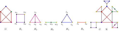
Figure 1: The generalized corona of $G$ and $\mathcal{H}$ constrained by $\mathcal{T}$

The rest of the paper is arranged as follows: In Section 2, we define the coronal of a matrix constrained by an index set and the coronal of a graph constrained by a vertex subset. We determine the coronal of some special kind of matrices. Also, we obtain the coronal of a matrix constrained by an arbitrary index set in terms of the coronal of some other matrix related to the given matrix. Using these, we determine the coronal of the graphs constrained by some of their vertex subsets obtained by the unary graph operations in $\mathcal{U}$, when the base graph is regular, the coronal of a semi-regular bipartite graph, the complete graph, complete bipartite graphs. In Section 3 and 4, we determine the characteristic polynomials of the adjacency and Laplacian matrices of the generalized corona of graphs constrained by vertex subsets, respectively. Further, we deduce the characteristic polynomials of the adjacency and the Laplacian matrices of some existing corona of graphs and the new variants of corona of graphs.

2 Coronal of a matrix constrained by an index set

McLeman et al. introduced the notion of coronal of a graph:

Definition 2.1.

([24]) Let $H$ be a graph with $n$ vertices. Then the sum of the entries of the matrix $(xI_{n}-A(H))^{-1}$ is said to be the coronal $\Gamma_{H}(x)$ of $H$. This can be calculated as

$$\Gamma_{H}(x)=J_{1\times n}(xI_{n}-A(H))^{-1}J_{n\times 1}.$$

Cui and Tian generalized this concept as follows:

Definition 2.2.

([7]) Let $G$ be a graph of with $n$ vertices and $M$ be a graph matrix of $G$. Then the sum of the entries of the matrix $(xI_{n}-M)^{-1}$ is said to be the $M$-coronal of $G$, and is denoted by $\Gamma_{M}(x)$. That is

$$\Gamma_{M}(x)=J_{1\times n}(xI_{n}-M)^{-1}J_{n\times 1}.$$

For a subset $B$ of a set $A=\{u_{1},u_{2},\ldots,u_{n}\}$, the indicator vector of $B$ (with respect to $A$) is a $0-1$ vector of length $n$ in which the $i$-th coordinate is 1 or 0, according as $u_{i}\in B$ or $u_{i}\notin B$, and it is denoted by $\mathbf{r}_{B}$. For a matrix $M\in M_{n}(\mathbb{R})$ and an index set $\alpha\subseteq\{1,2\ldots,n\}$, the principal submatrix of $M$ formed by $\alpha$ is the (sub)matrix of entries that lie in the rows and columns indexed by $\alpha$.

In the following definition, we introduce the notion of coronal of a matrix constrained by an index set, which generalizes Definition 2.2.

Definition 2.3.

Let $M\in M_{n}(\mathbb{R})$ and $\alpha\subseteq\{1,2,\ldots,n\}$ be an index set. Then the coronal of $M$ constrained by $\alpha$, denoted by $\Gamma_{M}^{\alpha}(x)$, is defined as the sum of all entries in the principal submatrix of $(xI_{n}-M)^{-1}$ formed by $\alpha$. Notice that this can be calculated by

$$\Gamma_{M}^{\alpha}(x)=\mathbf{r}_{\alpha}(xI_{n}-M)^{-1}\mathbf{r}_{\alpha}^{T}.$$

In the above definition, $xI_{n}-M$ is viewed as a matrix over the field of rational functions $\mathbb{C}(x)$. So $xI_{n}-M$ is invertible.

Remark 2.1.

1. If $\alpha=\{1,2,\ldots,n\}$, then we denote $\Gamma_{M}^{\alpha}(x)$ simply by $\Gamma_{M}(x)$ and we call this simply as the coronal of $M$. Notice that $\Gamma_{M}(x)=J_{n\times 1}(xI_{n}-M)^{-1}J_{1\times n}$.

2. If $H$ is a graph, $T\subseteq V(H)$ and $M$ is a graph matrix of $H$, then we call $\Gamma_{M}^{T}(x)$ as the $M$-coronal of $H$ constrained by the vertex subset $T$. If $T=V(H)$, then $\Gamma_{M}^{T}(x)=\Gamma_{M}(x)$. For $M=A(H)$ (resp. $L(H)$, $Q(H)$), we call $\Gamma_{M}^{T}(x)$ as the coronal (resp. $L$-coronal, $Q$-coronal) of $H$ constrained by the vertex subset $T$.

3. If $\alpha=\{i\}$, then we denote $\Gamma_{M}^{\alpha}(x)$ simply by $\Gamma_{M}^{i}(x)$. Notice that $\Gamma_{M}^{i}(x)$ is the $i$-th diagonal entry of the matrix $(xI_{n}-M)^{-1}$.

The following result gives the coronal of a matrix $M\in\mathcal{R}_{n\times n}(s)$ for some $s\in\mathbb{R}$.

Proposition 2.1.

([7, pro 2]) If $M\in\mathcal{R}_{n\times n}(s)$, then $\Gamma_{M}(x)=\displaystyle\frac{n}{x-s}$.

In the next result, we show that the coronal of a matrix is invariant under the rearrangement of the same rows and columns of the matrix.

Proposition 2.2.

If $A$ and $B$ are square matrices of order $n$ such that $PAP^{T}=B$ for a permutation matrix $P$, then $\Gamma_{A}(x)=\Gamma_{B}(x)$.

Proof.

$$\Gamma_{A}(x) = J_{1\times n}(xI_{n}-A)^{-1}J_{n\times 1}$$

$$= J_{1\times n}(xI_{n}-P^{T}BP)^{-1}J_{n\times 1}$$

$$= J_{1\times n}P^{T}(xI_{n}-B)^{-1}PJ_{n\times 1}$$

$$= J_{1\times n}(xI_{n}-B)^{-1}J_{n\times 1}$$

$$= \Gamma_{B}(x).$$

∎

In the following result, we obtain the coronal of a matrix, which satisfies some special constraints.

Theorem 2.1.

Let $A$ be square matrix of order $n$ such that

$$A=\begin{bmatrix}A_{1}&A_{2}\\ A_{3}&A_{4}\end{bmatrix},$$

where $A_{1}\in\mathcal{R}_{n_{1}\times n_{1}}(a_{1})$, $A_{2}\in\mathcal{R}_{n_{1}\times n_{2}}(a_{2})$, $A_{3}\in\mathcal{R}_{n_{2}\times n_{1}}(a_{3})$ and $A_{4}\in\mathcal{R}_{n_{2}\times n_{2}}(a_{4})$. Then

$$\Gamma_{A}(x)=\displaystyle\frac{(n_{1}+n_{2})x+n_{1}(a_{2}-a_{4})+n_{2}(a_{3}-a_{1})}{x^{2}-(a_{1}+a_{4})x+a_{1}a_{4}-a_{2}a_{3}}.$$ (2.1)

Proof.

It can be verified that

$$\Gamma_{A}(x) = [J_{1\times n_{1}}~{}J_{1\times n_{2}}](xI_{n_{1}+n_{2}}-A)^{-1}[J_{1\times n_{1}}~{}J_{1\times n_{2}}]^{T}.$$ (2.2)

By using [15, (0.7.3.1)], we have

$$(xI_{n_{1}+n_{2}}-A)^{-1}=\begin{bmatrix}A_{1}^{\prime}&-A_{2}^{\prime}\\ -A_{3}^{\prime}&A_{4}^{\prime}\end{bmatrix},$$ (2.3)

where

$A_{1}^{\prime}=\left(xI_{n_{1}}-A_{1}-A_{2}\left[xI_{n_{2}}-A_{4}\right]^{-1}A_{3}\right)^{-1}$,

$A_{2}^{\prime}=(xI_{n_{1}}-A_{1})^{-1}A_{2}\left(A_{3}[xI_{n_{1}}-A_{1}]^{-1}A_{2}-\left[xI_{n_{2}}-A_{4}\right]\right)^{-1}$,

$A_{3}^{\prime}=\left(A_{3}[xI_{n_{1}}-A_{1}]^{-1}A_{2}-\left[xI_{n_{2}}-A_{4}\right]\right)^{-1}A_{3}(xI_{n_{1}}-A_{1})^{-1}$,

$A_{4}^{\prime}=\left(xI_{n_{2}}-A_{4}-A_{3}[xI_{n_{1}}-A_{1}]^{-1}A_{2}\right)^{-1}$.

So, (2.2) becomes,

$$\Gamma_{A}(x) = S_{1}-S_{2}-S_{3}+S_{4},$$ (2.4)

where $S_{1}=J_{1\times n_{1}}A_{1}^{\prime}J_{n_{1}\times 1}$, $S_{2}=J_{1\times n_{1}}A_{2}^{\prime}J_{n_{2}\times 1}$, $S_{3}=J_{1\times n_{2}}A_{3}^{\prime}J_{n_{1}\times 1}$, $S_{4}=J_{1\times n_{2}}A_{4}^{\prime}J_{n_{2}\times 1}.$

Since $A_{1}\in\mathcal{R}_{n_{1}\times n_{1}}(a_{1})$, $A_{2}\in\mathcal{R}_{n_{1}\times n_{2}}(a_{2})$, $A_{3}\in\mathcal{R}_{n_{2}\times n_{1}}(a_{3})$ and $A_{4}\in\mathcal{R}_{n_{2}\times n_{2}}(a_{4})$, we have

$$A_{1}J_{n_{1}\times 1}=a_{1}J_{n_{1}\times 1}$$ (2.5)

$$A_{2}J_{n_{2}\times 1}=a_{2}J_{n_{1}\times 1}$$ (2.6)

$$A_{3}J_{n_{1}\times 1}=a_{3}J_{n_{2}\times 1}$$ (2.7)

$$A_{4}J_{n_{2}\times 1}=a_{4}J_{n_{2}\times 1}.$$ (2.8)

Also notice that, the sum of the entries in each row of $(xI_{n_{1}}-A_{1})^{-1}$ is equal to $\displaystyle\frac{1}{x-a_{1}}$. So,

$$(xI_{n_{1}}-A_{1})^{-1}J_{n_{1}\times 1}=\left(\displaystyle\frac{1}{x-a_{1}}\right)J_{n_{1}\times 1}.$$ (2.9)

Similarly,

$$(xI_{n_{2}}-A_{4})^{-1}J_{n_{2}\times 1}=\left(\displaystyle\frac{1}{x-a_{4}}\right)J_{n_{2}\times 1}.$$ (2.10)

By using (2.7), (2.10) and (2.6), we have

$$\left(A_{2}(xI_{n_{2}}-A_{4})^{-1}A_{3}\right)J_{n_{1}\times 1} = A_{2}\left(xI_{n_{2}}-A_{4}\right)^{-1}\left(A_{3}J_{n_{1}\times 1}\right)$$ (2.11)

$$= a_{3}A_{2}(xI_{n_{2}}-A_{4})^{-1}J_{n_{2}\times 1}$$

$$= \left(\displaystyle\frac{a_{3}}{x-a_{4}}\right)A_{2}J_{n_{2}\times 1}$$

$$= \left(\displaystyle\frac{a_{2}a_{3}}{x-a_{4}}\right)J_{n_{1}\times 1}.$$

Similarly, we get

$$\left(A_{3}(xI_{n_{1}}-A_{1})^{-1}A_{2}\right)J_{n_{2}\times 1} = \left(\displaystyle\frac{a_{2}a_{3}}{x-a_{1}}\right)J_{n_{2}\times 1}.$$ (2.12)

So by (2.5) and (2.11), we have

$$\left[xI_{n_{1}}-A_{1}-A_{2}(xI_{n_{2}}-A_{4})^{-1}A_{3}\right]J_{n_{1}\times 1} = \left(x-a_{1}-\displaystyle\frac{a_{2}a_{3}}{x-a_{4}}\right)J_{n_{1}\times 1}$$

$$= \left(\displaystyle\frac{x^{2}-(a_{1}+a_{4})x+a_{1}a_{4}-a_{2}a_{3}}{x-a_{4}}\right)J_{n_{1}\times 1}.$$

Consequently,

$$\left[xI_{n_{1}}-A_{1}-A_{2}(xI_{n_{2}}-A_{4})^{-1}A_{3}\right]^{-1}J_{n_{1}\times 1} = \left(\displaystyle\frac{x-a_{4}}{x^{2}-(a_{1}+a_{4})x+a_{1}a_{4}-a_{2}a_{3}}\right)J_{n_{1}\times 1}.$$

So, we have,

$$S_{1} = \displaystyle\frac{n_{1}(x-a_{4})}{x^{2}-(a_{1}+a_{4})x+a_{1}a_{4}-a_{2}a_{3}}.$$ (2.13)

Similarly, we get

$$S_{4} = \displaystyle\frac{n_{2}(x-a_{1})}{x^{2}-(a_{1}+a_{4})x+a_{1}a_{4}-a_{2}a_{3}}.$$

Now, by using (2.12) and (2.10), we have

$$\left\{A_{3}[I_{n_{1}}-A_{1}]^{-1}A_{2}-\left(xI_{n_{2}}-A_{4}\right)\right\}^{-1}J_{n_{2}\times 1} = \displaystyle\frac{1}{\displaystyle\left(\frac{a_{2}a_{3}}{x-a_{1}}\right)-(x-a_{4})}J_{n_{2}\times 1}$$

$$= \displaystyle\frac{x-a_{1}}{x^{2}-(a_{1}+a_{4})x+a_{1}a_{4}-a_{2}a_{3}}J_{n_{2}\times 1}$$

. (2.14)

Using (2.9) and (2.14), we get

$$S_{2} = J_{1\times n_{1}}(xI_{n_{1}}-A_{1})^{-1}A_{2}\left\{A_{3}(I_{n_{1}}-A_{1})^{-1}A_{2}-\left(xI_{n_{2}}-A_{4}\right)\right\}^{-1}J_{n_{2}\times 1}$$

$$= \left(\frac{1}{x-a_{1}}\right)J_{1\times n_{1}}A_{2}\left(\frac{x-a_{1}}{x^{2}-(a_{1}+a_{4})x+a_{1}a_{4}-a_{2}a_{3}}\right)J_{n_{1}\times 1}$$

$$= \left(\frac{a_{2}}{x^{2}-(a_{1}+a_{4})x+a_{1}a_{4}-a_{2}a_{3}}\right)J_{1\times n_{1}}J_{n_{1}\times 1}$$

$$= \frac{n_{1}a_{2}}{x^{2}-(a_{1}+a_{4})x+a_{1}a_{4}-a_{2}a_{3}}.$$

Also, we get

$$S_{3} = J_{1\times n_{2}}\left\{A_{3}(xI_{n_{1}}-A_{1})^{-1}A_{2}-\left(xI_{n_{2}}-A_{4}\right)\right\}^{-1}A_{3}(xI_{n_{1}}-A_{1})^{-1}J_{n_{1}\times 1}$$

$$= J_{1\times n_{1}}\left(\frac{x-a_{1}}{x^{2}-(a_{1}+a_{4})x+a_{1}a_{4}-a_{2}a_{3}}\right)A_{3}\left(\frac{1}{x-a_{1}}\right)J_{n_{2}\times 1}$$

$$= \left(\frac{a_{3}}{x^{2}-(a_{1}+a_{4})x+a_{1}a_{4}-a_{2}a_{3}}\right)J_{1\times n_{2}}J_{n_{2}\times 1}$$

$$= \frac{n_{2}a_{3}}{x^{2}-(a_{1}+a_{4})x+a_{1}a_{4}-a_{2}a_{3}}.$$

Substituting the values of $S_{1},S_{2},S_{3}$ and $S_{4}$ in (2.4), we get the result. ∎

In view of Proposition 2.2, if a matrix $A^{\prime}$ can be transformed (by rearranging the same rows and columns of $A^{\prime}$) to the matrix $A$ of the form given in Theorem 2.1, then the coronal of $A^{\prime}$ can be determined by (2.15).

In the next result, we determine the coronal of a matrix constrained by an arbitrary index set in terms of the coronal of a matrix related to the given matrix. Also we prove that, the coronal of a matrix constrained by an arbitrary index set with $n_{1}$ elements is same as the coronal of a matrix obtained by a suitable rearrangement of the rows and columns of the given matrix constrained by the index set $\{1,2,\ldots,n_{1}\}$.

Theorem 2.2.

Let $A$ be a square matrix of order $n$ and let $\alpha=\{\alpha_{1},\alpha_{2},\ldots,\alpha_{n_{1}}\}\subseteq\{1,2,\ldots,n\}$. Consider the partitioned matrix

$$A^{\prime}=\begin{bmatrix}A_{1}&A_{2}\\ A_{3}&A_{4}\end{bmatrix},$$

where $A_{1}$ is the principal submatrix of $A$ formed by $\alpha$, $A_{2}$ is the submatrix of $A$ formed by the rows in $\alpha$ and the columns in $\alpha^{c}$, $A_{3}$ is the submatrix of $A$ formed by the rows in $\alpha^{c}$ and the columns in $\alpha$, and $A_{4}$ is the principal submatrix of $A$ formed by $\alpha^{c}$. Then

$$\Gamma_{A}^{\alpha}(x)=\Gamma_{A^{\prime}}^{\alpha^{\prime}}(x)=\Gamma_{M}(x),$$

where $M=A_{1}+A_{2}(xI_{n_{2}}-A_{4})^{-1}A_{3}\text{ and }\alpha^{\prime}=\{1,2,\ldots,n_{1}\}.$

Moreover, if $A_{1}\in\mathcal{R}_{n_{1}\times n_{1}}(a_{1})$, $A_{2}\in\mathcal{R}_{n_{1}\times n_{2}}(a_{2})$, $A_{3}\in\mathcal{R}_{n_{2}\times n_{1}}(a_{3})$ and $A_{4}\in\mathcal{R}_{n_{2}\times n_{2}}(a_{4})$, then

$$\Gamma_{A}^{\alpha}(x)=\displaystyle\frac{n_{1}(x-a_{4})}{x^{2}-(a_{1}+a_{4})x+a_{1}a_{4}-a_{2}a_{3}}.$$ (2.15)

Proof.

First we prove that $\Gamma_{A}^{\alpha}(x)=\Gamma_{A^{\prime}}^{\alpha^{\prime}}(x)$. Without loss of generality we assume that $\alpha_{1}<\alpha_{2}<\cdots<\alpha_{n_{1}}$. Let $p$ be a permutation on $\{1,2,\ldots,n\}$ such that $p(1)=\alpha_{1},p(2)=\alpha_{2},\ldots,p(n_{1})=\alpha_{n_{1}}$ and $P$ be the permutation matrix corresponding to $p$. Then we have, $A^{\prime}=PAP^{T}$. Notice that $[J_{1\times n_{1}}~{}\textbf{0}]$ is the indicator vector of $\alpha^{\prime}$. Now,

$$\Gamma_{A}^{\alpha}(x) = \mathbf{r}_{\alpha}(xI_{n}-A)^{-1}\mathbf{r}_{\alpha}^{T}$$

$$= \mathbf{r}_{\alpha}(xI_{n}-P^{T}A^{\prime}P)^{-1}\mathbf{r}_{\alpha}^{T}$$

$$= \mathbf{r}_{\alpha}P^{T}(xI_{n}-A^{\prime})^{-1}P\mathbf{r}_{\alpha}^{T}$$

$$= [J_{1\times n_{1}}~{}\textbf{0}](xI_{n}-A^{\prime})^{-1}[J_{1\times n_{1}}~{}\textbf{0}]^{T}$$

$$= \Gamma_{A^{\prime}}^{\alpha^{\prime}}(x).$$

Using (2.3), we have

$$\Gamma_{A^{\prime}}^{\alpha^{\prime}}(x) = [J_{1\times n_{1}}~{}\textbf{0}](xI_{n}-A^{\prime})^{-1}[J_{1\times n_{1}}~{}\textbf{0}]^{T}$$

$$= J_{1\times n_{1}}\left[xI_{n_{1}}-A_{1}-A_{2}(xI_{n_{2}}-A_{4})^{-1}A_{3}\right]^{-1}J_{n_{1}\times 1}$$

$$= J_{1\times n_{1}}\left[xI_{n_{1}}-M\right]^{-1}J_{n_{1}\times 1}$$

$$= \Gamma_{M}(x).$$

Consequently, we have $\Gamma_{A}^{\alpha}(x)=\Gamma_{A^{\prime}}^{\alpha^{\prime}}(x)=\Gamma_{M}(x).$

If $A_{1}\in\mathcal{R}_{n_{1}\times n_{1}}(a_{1})$, $A_{2}\in\mathcal{R}_{n_{1}\times n_{2}}(a_{2})$, $A_{3}\in\mathcal{R}_{n_{2}\times n_{1}}(a_{3})$ and $A_{4}\in\mathcal{R}_{n_{2}\times n_{2}}(a_{4})$, then by substituting the value of $S_{1}$ as given in (2.13) in (2), we get (2.15). This completes the proof. ∎

Next, we start to determine the coronals of some classes of graphs constrained by some of their vertex subsets by using the previous results. It is well-known that the adjacency matrices of the graph $U(G)$ for a graph $G$ and $U\in\mathcal{U}$ is of the form

$$\begin{bmatrix}A_{1}&A_{2}\\ A_{3}&A_{4}\end{bmatrix},$$

where $A_{1}$, $A_{2}$, $A_{4}$ are as mentioned in the first row against each of these graphs in Table LABEL:table_coronals_of_various_graphs and $A_{3}=A_{2}^{T}$.

Corollary 2.1.

Let $G$ be an $r$-regular graph with $n$ vertices. Then the coronals of the graph $U(G)$, where $U\in\mathcal{U}$ constrained by some of their vertex subsets $T$ can be obtained by using Table LABEL:table_coronals_of_various_graphs: For the vertex subsets in first row given against each these graphs, apply the values $a_{1}$, $a_{2}$, $a_{3}$ and $a_{4}$ in (2.1) and for the vertex subsets $V(G)$ and $I(G)$ in second and third rows given against each of these graphs, apply the values $a_{1}$, $a_{2}$, $a_{3}$ and $a_{4}$ in (2.15). Notice that in each of these cases, $A_{3}=A_{2}^{T}$.

Table 1: The necessary entities to obtain the coronal of some graphs constrained by their vertex subsets

S. No	Graph ($G^{\prime}$)	Vertex subset $T$	$A_{1}$	$A_{2}$	$A_{4}$	$a_{1}$	$a_{2}$	$a_{3}$	$a_{4}$
1.	Subdivision graph of $G$	$V(G^{\prime})$	0	$B(G)$	0	0	$r$	2	0
		$V(G)$	0	$B(G)$	0	0	$r$	2	0
		$I(G)$	0	$B(G)^{T}$	0	0	2	$r$	0
2.	$R$-graph of $G$	$V(G^{\prime})$	$A(G)$	$B(G)$	0	$r$	$r$	2	0
		$V(G)$	$A(G)$	$B(G)$	0	$r$	$r$	2	0
		$I(G)$	0	$B(G)^{T}$	$A(G)$	0	2	$r$	$r$
3.	$\mathcal{Q}$-graph of $G$	$V(G^{\prime})$	0	$B(G)$	$A(\mathcal{L}(G))$	0	$r$	2	$2r-2$
		$V(G)$	0	$B(G)$	$A(\mathcal{L}(G))$	0	$r$	2	$2r-2$
		$I(G)$	$A(\mathcal{L}(G))$	$B(G)^{T}$	0	$2r-2$	$2$	$r$	0
4.	Central graph of $G$	$V(G^{\prime})$	$A(\overline{G})$	$B(G)$	0	$n-r-1$	$r$	2	0
		$V(G)$	$A(\overline{G})$	$B(G)$	0	$n-r-1$	$r$	2	0
		$I(G)$	0	$B(G)^{T}$	$A(\overline{G})$	0	2	$r$	$n-r-1$
5.	Total graph of $G$	$V(G^{\prime})$	$A(G)$	$B(G)$	$A(\mathcal{L}(G))$	$r$	$r$	$2$	$2r-2$
		$V(G)$	$A(G)$	$B(G)$	$A(\mathcal{L}(G))$	$r$	$r$	$2$	$2r-2$
		$I(G)$	$A(\mathcal{L}(G))$	$B(G)^{T}$	$A(G)$	$2r-2$	$2$	$r$	$r$
6.	Quasi-total graph of $G$	$V(G^{\prime})$	$A(\overline{G})$	$B(G)$	$A(\mathcal{L}(G))$	$n-r-1$	$r$	$2$	$2r-2$
		$V(G)$	$A(\overline{G})$	$B(G)$	$A(\mathcal{L}(G))$	$n-r-1$	$r$	$2$	$2r-2$
		$I(G)$	$A(\mathcal{L}(G))$	$B(G)^{T}$	$A(\overline{G})$	$2r-2$	$2$	$r$	$n-r-1$
7.	Duplicate graph of $G$	$V(G^{\prime})$	0	$A(G)$	0	$0$	$r$	$r$	0
		$V(G)$	0	$A(G)$	0	$0$	$r$	$r$	0
		$I(G)$	0	$A(G)$	0	0	$r$	$r$	$0$
8.	$C$-graph of $G$	$V(G^{\prime})$	$A(G)$	$I_{n}$	0	$r$	$1$	$1$	0
		$V(G)$	$A(G)$	$I_{n}$	0	$r$	$1$	$1$	0
		$I(G)$	0	$I_{n}$	$A(G)$	0	$1$	1	$r$
9.	$N$-graph of $G$	$V(G^{\prime})$	$A(G)$	$A(G)$	0	$r$	$r$	$r$	0
		$V(G)$	$A(G)$	$A(G)$	0	$r$	$r$	$r$	0
		$I(G)$	0	$A(G)$	$A(G)$	0	$r$	$r$	$r$
10.	point complete subdivision graph of $G$	$V(G^{\prime})$	$J_{n}-I_{n}$	$B(G)$	0	$n-1$	$r$	$2$	$0$
		$V(G)$	$J_{n}-I_{n}$	$B(G)$	0	$n-1$	$r$	$2$	$0$
		$I(G)$	0	$B(G)^{T}$	$J_{n}-I_{n}$	$0$	$2$	$r$	$n-1$
11.	$\mathcal{Q}$- complemented graph of $G$	$V(G^{\prime})$	0	$B(G)$	$A(\overline{\mathcal{L}(G)})$	0	$r$	2	$m^{\prime}-2r+1$
		$V(G)$	0	$B(G)$	$A(\overline{\mathcal{L}(G)})$	0	$r$	2	$m^{\prime}-2r+1$
		$I(G)$	$A(\overline{\mathcal{L}(G)})$	$B(G)^{T}$	0	$m^{\prime}-2r+1$	$2$	$r$	0
12.	Total complemented graph of $G$	$V(G^{\prime})$	$A(G)$	$B(G)$	$A(\overline{\mathcal{L}(G)})$	$r$	$r$	$2$	$m^{\prime}-2r+1$
		$V(G)$	$A(G)$	$B(G)$	$A(\overline{\mathcal{L}(G)})$	$r$	$r$	$2$	$m^{\prime}-2r+1$
		$I(G)$	$A(\overline{\mathcal{L}(G)})$	$B(G)^{T}$	$A(G)$	$m^{\prime}-2r+1$	$2$	$r$	$r$
13.	Quasitotal complemented graph of $G$	$V(G^{\prime})$	$A(\overline{G})$	$B(G)$	$A(\overline{\mathcal{L}(G)})$	$n-r-1$	$r$	2	$m^{\prime}-2r+1$
		$V(G)$	$A(\overline{G})$	$B(G)$	$A(\overline{\mathcal{L}(G)})$	$n-r-1$	$r$	2	$m^{\prime}-2r+1$
		$I(G)$	$A(\overline{\mathcal{L}(G)})$	$B(G)^{T}$	$A(\overline{G})$	$m^{\prime}-2r+1$	$2$	$r$	$n-r-1$
14.	Complete $\mathcal{Q}$- complemented graph of $G$	$V(G^{\prime})$	$J_{n}-I_{n}$	$B(G)$	$A(\overline{\mathcal{L}(G)})$	$n-1$	$r$	2	$m^{\prime}-2r+1$
		$V(G)$	$J_{n}-I_{n}$	$B(G)$	$A(\overline{\mathcal{L}(G)})$	$n-1$	$r$	2	$m^{\prime}-2r+1$
		$I(G)$	$A(\overline{\mathcal{L}(G)})$	$B(G)^{T}$	$J_{n}-I_{n}$	$m^{\prime}-2r+1$	$2$	$r$	$n-1$
15.	Complete subdivision graph of $G$	$V(G^{\prime})$	0	$B(G)$	$J_{m}-I_{m}$	0	$r$	2	$m-1$
		$V(G)$	0	$B(G)$	$J_{m}-I_{m}$	0	$r$	2	$m-1$
		$I(G)$	$J_{m}-I_{m}$	$B(G)^{T}$	0	$m-1$	2	$r$	0
16.	Complete $R$-graph of $G$	$V(G^{\prime})$	$A(G)$	$B(G)$	$J_{m}-I_{m}$	$r$	$r$	2	$m-1$
		$V(G)$	$A(G)$	$B(G)$	$J_{m}-I_{m}$	$r$	$r$	2	$m-1$
		$I(G)$	$J_{m}-I_{m}$	$B(G)^{T}$	$A(G)$	$m-1$	2	$r$	$r$
17.	Complete central graph of $G$	$V(G^{\prime})$	$A(\overline{G})$	$B(G)$	$J_{m}-I_{m}$	$n-r-1$	$r$	2	$m-1$
		$V(G)$	$A(\overline{G})$	$B(G)$	0	$n-r-1$	$r$	2	$m-1$
		$I(G)$	$J_{m}-I_{m}$	$B(G)^{T}$	$A(\overline{G})$	$m-1$	2	$r$	$n-r-1$
18.	Fully complete subdivision graph of $G$	$V(G^{\prime})$	$J_{n}-I_{n}$	$B(G)$	$J_{m}-I_{m}$	$n-1$	$r$	2	$m-1$
		$V(G)$	$J_{n}-I_{n}$	$B(G)$	$J_{m}-I_{m}$	$n-1$	$r$	2	$m-1$
		$I(G)$	$J_{m}-I_{m}$	$B(G)^{T}$	$J_{n}-I_{n}$	$m-1$	2	$r$	$n-1$

Corollary 2.2.

If $G$ is a semi-regular bipartite graph with bipartition $(X,Y)$ and parameters $(n_{1},n_{2},r_{1},r_{2})$, then we have the following.

1. $\displaystyle\Gamma_{G}(x)=\frac{(n_{1}+n_{2})x+2n_{1}r_{1}}{x^{2}-r_{1}r_{2}},$

2. $\displaystyle\Gamma_{G}^{X}(x)=\frac{n_{1}x}{x^{2}-r_{1}r_{2}}.$

Proof.

Notice that,

$$A(G)=\begin{bmatrix}\textbf{0}_{n_{1}}&W_{n_{1}\times n_{2}}\\ W_{n_{2}\times n_{1}}&\textbf{0}_{n_{2}}\end{bmatrix},$$ (2.17)

where $W\in\mathcal{RC}_{n_{1}\times n_{2}}(r_{1},r_{2})$. Taking $a_{1}=0$, $a_{2}=r_{1}$, $a_{3}=r_{2}$ and $a_{4}=0$ in (2.1) and (2.15), and using the fact that $n_{1}r_{1}=n_{2}r_{2}$, we get the proof of parts (1) and (2), respectively. ∎

For two graphs $H_{1}$ and $H_{2}$, their join, denoted by $H_{1}\vee H_{2}$, is the graph obtained by taking one copy of $H_{1}$ and $H_{2}$, and joining each vertex of $H_{1}$ to all the vertices of $H_{2}$.

Corollary 2.3.

([24, Proposition 17]) If $H_{1}$ is an $r_{1}$-regular graph with $n_{1}$ vertices and $H_{2}$ is an $r_{2}$-regular graph with $n_{2}$ vertices, then

$$\Gamma_{H_{1}\vee H_{2}}(x)=\displaystyle\frac{(n_{1}+n_{2})x+n_{1}(n_{2}-r_{2})+n_{2}(n_{1}-r_{1})}{x^{2}-(r_{1}+r_{2})x+r_{1}r_{2}-n_{1}n_{2}}.$$

Proof.

Notice that

$$A(H_{1}\vee H_{2})=\begin{bmatrix}A(H_{1})&J_{n_{1}\times n_{2}}\\ J_{n_{2}\times n_{1}}&A(H_{2})\end{bmatrix}.$$

Since $H_{1},H_{2}$ are $r_{1}$, $r_{2}$-regular graphs, respectively, we have $A(H_{1})\in\mathcal{R}_{n_{1}\times n_{1}}(r_{1})$ and $A(H_{2})\in\mathcal{R}_{n_{2}\times n_{2}}(r_{2})$. So, taking $a_{1}=r_{1},a_{2}=n_{2},a_{3}=n_{1}$ and $a_{4}=r_{2}$ in (2.1), we obtain the result. ∎

Corollary 2.4.

If $T$ is a vertex subset of $K_{n}$ with $|T|=t$, then $\Gamma_{K_{n}}^{T}(x)=\displaystyle\frac{t(x-n+t+1)}{(x+1)(x-n+1)}$.

Proof.

We arrange the rows and columns of $A(K_{n})$ by the vertices in $T$ and the remaining vertices of $K_{n}$, respectively. Then we have

$$A(K_{n})=\begin{bmatrix}A(K_{t})&J_{t\times(n-t)}\\ J_{(n-t)\times t}&A(K_{n-t})\end{bmatrix}.$$ (2.18)

Taking $a_{1}=t-1$, $a_{2}=n-t$, $a_{3}=t$ and $a_{4}=n-t-1$ in (2.15), we get the result. ∎

The following result is established in [28].

Theorem 2.3.

([28, Theorem 4]) The adjoint matrix of $xI_{p+q}-A(K_{p,q})$ is given in the form of a partitioned matrix by

$\begin{bmatrix}P_{K_{p-1,q}}(x)I_{p}+qx^{p+q-3}(J_{p}-I_{p})&x^{p+q-2}J_{p\times q}\\ x^{p+q-2}J_{q\times p}&P_{K_{p,q-1}}(x)I_{q}+px^{p+q-3}(J_{q}-I_{q})\end{bmatrix}$.

Proposition 2.3.

Consider the complete bipartite graph $K_{p,q}$ with a bipartition $(X,Y)$ be such that $|X|=p$. Let $S_{1}\subseteq X$ and $S_{2}\subseteq Y$ be such that $|S_{1}|=s_{1}$ and $|S_{2}|=s_{2}$. Then

$$\Gamma_{K_{p,q}}^{S_{1}\cup S_{2}}(x)=\displaystyle\frac{(s_{1}+s_{2})x^{2}+2s_{1}s_{2}x-(s_{1}+s_{2})pq+s_{1}^{2}q+s_{2}^{2}p}{x(x^{2}-pq)}.$$

Proof.

Since, $\Gamma_{K_{p,q}}^{S_{1}\cup S_{2}}$ is the sum of all entries in the principal submatrix of $(xI_{p+q}-A(K_{p,q}))^{-1}$ formed by the vertices in $S_{1}\cup S_{2}$, by using Theorem 2.3, we have

$$\Gamma_{K_{p,q}}^{S_{1}\cup S_{2}}(x)=\displaystyle\frac{1}{P_{K_{p,q}}(x)} \left(s_{1}P_{K_{p-1,q}}(x)+q(s_{1}^{2}-s_{1})x^{p+q-3}+2s_{1}s_{2}x^{p+q-2}\right.$$

$$\left.+s_{2}P_{K_{p,q-1}}(x)+p(s_{2}^{2}-s_{2})x^{p+q-3}\right).$$ (2.19)

Using the fact that $P_{K_{p,q}}(x)=x^{p+q-2}(x^{2}-pq)$ in the above equation, we get the result. ∎

We deduce the following result, by taking $S_{1}=X$ and $S_{2}=Y$ in Proposition 2.3.

Corollary 2.5.

([24, Proposition 8]) $\Gamma_{K_{p,q}}(x)=\displaystyle\frac{(p+q)x+2pq}{x^{2}-pq}.$

3 The characteristic polynomial of the adjacency matrix of $G\circledast_{\mathcal{T}}\mathcal{H}$

In the rest of the paper, we assume the following unless we specifically mention otherwise: $G$ is a graph with $V(G)=\{v_{1},v_{2},\ldots,v_{n}\}$, $\mathcal{H}=(H_{1}$ is a sequence of $n$ graphs $H_{1},H_{2},\ldots,H_{n}$ with $|V(H_{i})|=h_{i}$ for $i=1,2,\ldots,n$ and $\mathcal{T}$ is a sequence of sets $T_{1},T_{2},\ldots,T_{n}$, where $T_{i}\subseteq V(H_{i})$ with $|T_{i}|=t_{i}$ for $i=1,2,\ldots,n$. Let $\mathbf{r_{i}}:=\mathbf{r_{T_{i}}}$ for $i=1,2,\ldots,n$.

In this section, first we determine the characteristic polynomial of the adjacency matrix of the generalized corona of $G$ and $\mathcal{H}$ constrained by $\mathcal{T}$, which is one of the main result of this paper.

The following result is used throughout this paper.

Theorem 3.1.

([2]) Let $A$ be a matrix partitioned as

$$A=\begin{bmatrix}A_{1}&A_{2}\\ A_{3}&A_{4}\end{bmatrix},$$

where $A_{1},A_{4}$ are square invertible matrices. Then

$$|A| =|A_{4}||A_{1}-A_{2}A_{4}^{-1}A_{3}|=|A_{1}||A_{4}-A_{3}A_{1}^{-1}A_{2}|.$$

Theorem 3.2.

The characteristic polynomial of the adjacency matrix of $G\circledast_{\mathcal{T}}\mathcal{H}$ is

$$P_{G\circledast_{\mathcal{T}}\mathcal{H}}(x)=\left\{\prod_{i=1}^{n}P_{H_{i}}(x)\right\}\times\left|xI_{n}-A(G)-U_{A}\right|,$$

where $U_{A}=\begin{bmatrix}\Gamma_{H_{1}}^{T_{1}}(x)&0&\cdots&0\\ 0&\Gamma_{H_{2}}^{T_{2}}(x)&\cdots&0\\ \vdots&\vdots&\ddots&\vdots\\ 0&0&\cdots&\Gamma_{H_{n}}^{T_{n}}(x)\end{bmatrix}$.

Proof.

We arrange the rows and columns of the adjacency matrix of $G\circledast_{\mathcal{T}}\mathcal{H}$ by the vertices of $G,H_{1},H_{2},\ldots,H_{n},$ respectively. Then

$$A(G\circledast_{\mathcal{T}}\mathcal{H})=\begin{bmatrix}A(G)&C\\ C^{T}&E\end{bmatrix},$$

where

$$E=\begin{bmatrix}A(H_{1})&\textbf{0}&\cdots&\textbf{0}\\ \textbf{0}&A(H_{2})&\cdots&\textbf{0}\\ \vdots&\vdots&\ddots&\vdots\\ \textbf{0}&\textbf{0}&\cdots&A(H_{n})\end{bmatrix}_{p\times p}~{}~{}\text{and}~{}~{}C=\begin{bmatrix}\mathbf{r_{1}}&\textbf{0}&\cdots&\textbf{0}\\ \textbf{ 0}&\mathbf{r_{2}}&\cdots&\textbf{0}\\ \vdots&\vdots&\ddots&\vdots\\ \textbf{0}&\textbf{0 }&\cdots&\mathbf{r_{n}}\end{bmatrix}_{n\times p}.$$

with $p=\displaystyle\sum_{i=1}^{n}h_{i}$. By using Theorem 3.1, we have

$$P_{G\circledast_{\mathcal{T}}\mathcal{H}}(x) = \begin{vmatrix}xI_{n}-A(G)&-C\\ -C^{T}&xI_{p}-E\end{vmatrix}$$ (3.1)

$$= \left|xI_{p}-E\right|\times\left|xI_{n}-A(G)-C(xI_{p}-E)^{-1}C^{T}\right|.$$

It is not hard to see that,

$$\left|xI_{p}-E\right|=\displaystyle\prod_{i=1}^{n}\left|xI_{h_{i}}-A(H_{i})\right|=\displaystyle\prod_{i=1}^{n}P_{H_{i}}(x).$$

Also,

$C(xI_{p}-E)^{-1}C^{T}$

$$= C\begin{bmatrix}xI_{h_{1}}-A(H_{1})&\textbf{0}&\cdots&\textbf{0}\\ \textbf{0}&xI_{h_{2}}-A(H_{2})&\cdots&\textbf{0}\\ \vdots&\vdots&\ddots&\vdots\\ \textbf{0}&\textbf{0}&\cdots&xI_{h_{n}}-A(H_{n})\end{bmatrix}^{-1}C^{T}$$

$$= \begin{bmatrix}\mathbf{r_{1}}\left(xI_{h_{1}}-A(H_{1})\right)^{-1}\mathbf{r}^{T}_{\mathbf{1}}&0&\cdots&0\\ 0&\mathbf{r_{2}}\left(xI_{h_{2}}-A(H_{2})\right)^{-1}\mathbf{r}^{T}_{\mathbf{2}}&\cdots&0\\ \vdots&\vdots&\ddots&\vdots\\ 0&0&\cdots&\mathbf{r_{n}}\left(xI_{h_{n}}-A(H_{n})\right)^{-1}\mathbf{r}^{T}_{\mathbf{n}}\end{bmatrix}$$

$$= U_{A}.$$

Substituting these values in (3.1) we get the result. ∎

Theorem 3.2 shows that, the $A$-spectrum of $G\circledast_{\mathcal{T}}\mathcal{H}$ can be completely determined by the $A$-spectrum of the constituent graphs and their coronals constrained by the corresponding vertex subsets. In the following result, we show that, if all the coronals of $H_{i}$’s constrained by their corresponding subsets $T_{i}$ are equal, then the $A$-spectrum of $G\circledast_{\mathcal{T}}\mathcal{H}$ is same regardless of the order of $H_{i}$’s in $\mathcal{H}$. So, in this case, by interchanging the order of $H_{i}$’s in $\mathcal{H}$, we can get a family of $A$-cospectral graphs.

Corollary 3.1.

If $\Gamma_{H_{1}}^{T_{1}}(x)=\Gamma_{H_{2}}^{T_{2}}(x)=\cdots=\Gamma_{H_{n}}^{T_{n}}(x)$, then the characteristic polynomial of the adjacency matrix of $G\circledast_{\mathcal{T}}\mathcal{H}$ is

$$\left\{\prod_{i=1}^{n}P_{H_{i}}(x)\right\}\times\left\{\prod_{j=1}^{n}\left(x-\lambda_{j}(G)-\Gamma_{H_{1}}^{T_{1}}(x)\right)\right\}.$$

In the rest of this section, we consider some interesting graphs $H_{i}$’s whose adjacency matrices are $2\times 2$ block matrices with some special constraints.

Corollary 3.2.

Suppose for $i=1,2,\ldots,n$,

$$A(H_{i})=\begin{bmatrix}A_{1i}&A_{2i}\\ A_{2i}^{T}&A_{3i}\end{bmatrix},$$

where $A_{1i}\in\mathcal{R}_{r_{i}\times r_{i}}(a_{1})$, $A_{3i}\in\mathcal{R}_{s_{i}\times s_{i}}(a_{4})$ and $A_{2i}\in\mathcal{RC}_{r_{i}\times s_{i}}(a_{2},a_{3})$, with $r_{i}+s_{i}=|V(H_{i})|$. Then we have the following.

1. If $|V(H_{1})|=|V(H_{2})|=\cdots=|V(H_{n})|=h$ and $r_{1}=r_{2}=\cdots=r_{n}=t$, then the characteristic polynomial of the adjacency matrix of $G\circledast\mathcal{H}$ is

   $$\displaystyle\frac{\displaystyle\prod_{i=1}^{n}P_{H_{i}}(x)}{\left\{x^{2}-k_{1}x+k_{2}\right\}^{n}}\times \prod_{j=1}^{n}\left(x^{3}-\left\{k_{1}+\lambda_{j}(G)\right\}x^{2}+\left\{k_{1}\lambda_{j}(G)+k_{2}-h\right\}x\right.$$

   $$~{}~{}~{}~{}\left.-k_{2}\lambda_{j}(G)-t(a_{2}-a_{4})-(h-t)(a_{3}-a_{1})\right),$$ (3.2)

2. If for each $i=1,2,\ldots,n$, $A_{1i}$ is the adjacency matrix of the subgraph induced by $T_{i}$ in $H_{i}$ and $|T_{i}|=t$, then the characteristic polynomial of the adjacency matrix of $G\circledast_{\mathcal{T}}\mathcal{H}$ is

   $$\frac{\displaystyle\prod_{i=1}^{n}P_{H_{i}}(x)}{\left\{x^{2}-k_{1}x+k_{2}\right\}^{n}}\times\prod_{j=1}^{n}\left(x^{3}-\left\{k_{1}+\lambda_{j}(G)\right\}x^{2}+\left\{k_{1}\lambda_{j}(G)+k_{2}-t\right\}x-k_{2}\lambda_{j}(G)+ta_{4}\right),$$

where $k_{1}=a_{1}+a_{4}$, $k_{2}=a_{1}a_{4}-a_{2}a_{3}$.

Proof.

Taking $n_{1}=t$ and $n_{2}=h-t$ in (2.1) and (2.15), we have

$$\displaystyle\Gamma_{H_{i}}(x)=\displaystyle\frac{hx+t(a_{2}-a_{4})+(h-t)(a_{3}-a_{1})}{x^{2}-(a_{1}+a_{4})x+a_{1}a_{4}-a_{2}a_{3}}$$

and

$$\displaystyle\Gamma_{H_{i}}^{T_{i}}(x)=\frac{t(x-a_{4})}{x^{2}-(a_{1}+a_{4})x+a_{1}a_{4}-a_{2}a_{3}}$$

for each $i=1,2,\ldots,n$. So the proof follows bu using these values in Corollary 3.1. ∎

Remark 3.1.

1. For each $i=1,2,\ldots,n$, let $H_{i}$ = $S(H_{i}^{\prime})$, where $H_{i}^{\prime}$ is an $r$-regular graph with $h$ vertices. Then we can obtain the characteristic polynomial of the adjacency matrix of $G\circledast\mathcal{H}$ by applying the values of $a_{1},a_{2},a_{3},a_{4}$ as in the first row given against the subdivision graph in Table LABEL:table_coronals_of_various_graphs and using the characteristic polynomial of the adjacency matrix of $S(H_{i}^{\prime})$ [9, (2.32)], in Corollary 3.2; Further if $T_{i}=V(H_{i}^{\prime})$ or $I(H_{i}^{\prime})$ for each $i=1,2,\ldots,n$, then we can obtain the characteristic polynomial of the adjacency matrix of $G\circledast_{\mathcal{T}}\mathcal{H}$ by applying the values of $a_{1},a_{2},a_{3},a_{4}$ as in second and third rows given against the subdivision graph in Table LABEL:table_coronals_of_various_graphs, respectively, and using the characteristic polynomial of the adjacency matrix of $S(H_{i}^{\prime})$, in Corollary 3.2.

2. For each $i=1,2,\ldots,n$, if $H_{i}$ is one of the graph in $\mathcal{U}_{H_{i}^{\prime}}$ for an $r$-regular graph $H_{i}^{\prime}$ with $h$ vertices, and $T_{i}=V(H_{i}^{\prime})$ or $I(H_{i}^{\prime})$, then the characteristic polynomial of the adjacency matrix of $G\circledast\mathcal{H}$ and $G\circledast_{\mathcal{T}}\mathcal{H}$ can be obtained by the similar method described in the preceding part of this remark.

Corollary 3.3.

If $H_{i}$ is a semi-regular bipartite graph with bipartition $(X_{i},Y_{i})$ and parameters $(n_{1},n_{2},r_{1},r_{2})$ for $i=1,2,\ldots,n$, then we have the following.

1. The characteristic polynomial of the adjacency matrix of $G\circledast\mathcal{H}$ is

   $$\frac{\displaystyle\prod_{i=1}^{n}P_{H_{i}}(x)}{\left\{x^{2}-r_{1}r_{2}\right\}^{n}}\times\prod_{j=1}^{n}\left(x^{3}-\lambda_{j}(G)x^{2}-\left\{r_{1}r_{2}+n_{1}+n_{2}\right\}x+r_{1}r_{2}\lambda_{j}(G)+2n_{1}r_{1}\right).$$

2. If $T_{i}=X_{i}$ for each $i=1,2,\ldots,n$, then the characteristic polynomial of the adjacency matrix of $G\circledast_{\mathcal{T}}\mathcal{H}$ is

   $$\frac{\displaystyle\prod_{i=1}^{n}P_{H_{i}}(x)}{\left\{x^{2}-r_{1}r_{2}\right\}^{n}}\times\prod_{j=1}^{n}\left(x^{3}-\lambda_{j}(G)x^{2}-\left\{n_{1}+r_{1}r_{2}\right\}x+r_{1}r_{2}\lambda_{j}(G)\right).$$

Proof.

In view of (2.17), taking $t=n_{1}$, $h-t=n_{2}$, $a_{1}=0$, $a_{2}=r_{1}$, $a_{3}=r_{2}$ and $a_{4}=0$ in parts of (1) and (2) of Corollary 3.2, we get the proof of parts (1) and (2), respectively. ∎

Corollary 3.4.

If $H_{i}=K_{m}$ and $T_{i}$ is a vertex subset of $K_{m}$ with $|T_{i}|=t$ for each $i=1,2,\ldots,n$, then the $A$-spectrum of $G\circledast_{\mathcal{T}}\mathcal{H}$ is

1. $-1$ with multiplicity $n(m-2)$;

2. for $i=1,2,\ldots,n$, the roots of the polynomial

   $$x^{3}-\left\{m+\lambda_{i}(G)-2\right\}x^{2}+\left\{(m-2)\lambda_{i}(G)-m+1-t\right\}x+(m-1)\lambda_{i}(G)+t(m-t-1).$$

Proof.

In view of (2.18), taking $a_{1}=t-1$, $a_{2}=m-t$, $a_{3}=t$ and $a_{4}=m-t-1$ in Corollary 3.2(2), we get the result. ∎

Corollary 3.5.

Consider the complete bipartite graph $K_{p,q}$ with bipartition $(X,Y)$ such that $|X|=p$. Let $S_{1}\subseteq X$ and $S_{2}\subseteq Y$ with $|S_{1}|=s_{1}$ and $|S_{2}|=s_{2}$. If $H_{i}=K_{p,q}$ and $T_{i}=S_{1}\cup S_{2}$ for each $i=1,2,\ldots,n$, then the $A$-spectrum of $G\circledast_{\mathcal{T}}\mathcal{H}$ is

1. $0$ with multiplicity $n(p+q-3)$,

2. for $i=1,2,\ldots,n$, the roots of the polynomial

   $$x^{4}-\lambda_{i}(G)x^{3}-\left\{pq+s_{1}+s_{2}\right\}x^{2}+\left\{pq\lambda_{i}(G)-2s_{1}s_{2}\right\}x+(s_{1}+s_{2})pq-s_{1}^{2}q-s_{2}^{2}p.$$

Proof.

Applying Proposition 2.3 in Corollary 3.1, we get the result. ∎

4 The characteristic polynomial of the Laplacian matrix of $G\circledast_{\mathcal{T}}\mathcal{H}$

Notation 4.1.

Suppose $H$ is a graph with $h$ vertices, $T\subseteq V(H)$ and $\mathbf{r}_{T}=(r_{1},r_{2},\ldots,r_{{h}})$, then we denote the diagonal matrix whose diagonal entries are $r_{1},r_{2},\ldots,r_{{h}}$ by $R_{T}$. Also the characteristic polynomial of $L(H)+R_{T}$ is denoted by $L_{H}^{T}(x)$.

Theorem 4.1.

The characteristic polynomial of the Laplacian matrix of $G\circledast_{\mathcal{T}}\mathcal{H}$ is

$$L_{G\circledast_{\mathcal{T}}\mathcal{H}}(x)=\left\{\prod_{i=1}^{n}L_{H_{i}}^{T_{i}}(x)\right\}\times\left|xI_{n}-L(G)-U_{L}\right|,$$

where

$$U_{L}=\begin{bmatrix}t_{1}+\Gamma_{L(H_{1})+R_{T_{1}}}^{T_{1}}(x)&0&\cdots&0\\ 0&t_{2}+\Gamma_{L(H_{2})+R_{T_{2}}}^{T_{2}}(x)&\cdots&0\\ \vdots&\vdots&\ddots&\vdots\\ 0&0&\cdots&t_{n}+\Gamma_{L(H_{n})+R_{T_{n}}}^{T_{n}}(x)\end{bmatrix}.$$

Proof.

Notice that

$$L(G\circledast_{\mathcal{T}}\mathcal{H})=\begin{bmatrix}L(G)+N&-C\\ -C^{T}&E^{\prime}\end{bmatrix},$$

where $C$ is the matrix as in Theorem 3.2, $N=diag(t_{1},t_{2},\ldots,t_{n})$ and

$$E^{\prime}=\begin{bmatrix}L(H_{1})+R_{T_{1}}&\textbf{0}&\cdots&\textbf{0}\\ \textbf{0}&L(H_{2})+R_{T_{2}}&\cdots&\textbf{0}\\ \vdots&\vdots&\ddots&\vdots\\ \textbf{0}&\textbf{0}&\cdots&L(H_{n})+R_{T_{n}}\end{bmatrix}_{p\times p},$$

with $p=\displaystyle\sum_{i=1}^{n}h_{i}$. By using Theorem 3.1, we have

$$L_{G\circledast_{\mathcal{T}}\mathcal{H}}(x) = \begin{vmatrix}xI_{n}-L(G)-N&C\\ C^{T}&xI_{p}-E^{\prime}\end{vmatrix}$$ (4.1)

$$= \left|xI_{p}-E^{\prime}\right|\times\left|xI_{n}-L(G)-N-C(xI_{p}-E^{\prime})^{-1}C^{T}\right|.$$

It is not hard to see that,

$$\left|xI_{p}-E^{\prime}\right|=\displaystyle\prod_{i=1}^{n}\left|xI_{h_{i}}-L(H_{i})-R_{T_{i}}\right|=\prod_{i=1}^{n}L_{H_{i}}^{T_{i}}(x).$$

Also,
$C(xI_{p}-E^{\prime})^{-1}C^{T}$

$$= C\begin{bmatrix}xI_{h_{1}}-L(H_{1})-R_{T_{1}}&\textbf{0}&\cdots&\textbf{ 0}&\\ \textbf{0}&xI_{h_{2}}-L(H_{2})-R_{T_{2}}&\cdots&\textbf{0}\\ \vdots&\vdots&\ddots&\vdots\\ \textbf{ 0}&\textbf{0}&\cdots&xI_{h_{n}}-L(H_{n})-R_{T_{n}}\end{bmatrix}^{-1}C^{T}$$

$$= \begin{bmatrix}\Gamma_{L(H_{1})+R_{T_{1}}}^{T_{1}}(x)&0&\cdots&0\\ 0&\Gamma_{L(H_{2})+R_{T_{2}}}^{T_{2}}(x)&\cdots&0\\ \vdots&\vdots&\ddots&\vdots\\ 0&0&\cdots&\Gamma_{L(H_{n})+R_{T_{n}}}^{T_{n}}(x)\end{bmatrix}.$$

So we have, $N+C(xI_{p}-E^{\prime})^{-1}C^{T}=U_{L}.$ Substituting these values in (4.1) we get the result. ∎

Note 4.1.

The characteristic polynomial of the signless Laplacian matrix of $G\circledast_{\mathcal{T}}\mathcal{H}$ can be obtained by using the analogous method described in Theorem 4.1. Consequently, the rest of the results proved in this section can also be deduced for the signless Laplacian matrix (with additional constraints $A_{1i}\in\mathcal{R}_{t\times t}(a_{1})$ and $A_{3i}\in\mathcal{R}_{(h_{i}-t)\times(h_{i}-t)}(a_{4})$ in Corollary 4.2). The details are omitted.

Theorem 4.1 shows that, the characteristic polynomial of the Laplacian matrix of $G\circledast_{\mathcal{T}}\mathcal{H}$ can be completely determined by the $L$-spectrum of $G$, the polynomials $L_{H_{i}}^{T_{i}}(x)$ and the coronals of the matrices $L(H_{i})+R_{T_{i}}$ constrained by their vertex subsets. The following is a direct consequence of Theorem 4.1, which shows that, if all the coronals $\Gamma_{L(H_{i})+R_{T_{i}}}^{T_{i}}(x)$ are equal, then the $L$-spectrum of $G\circledast_{\mathcal{T}}\mathcal{H}$ is same regardless of the order of $H_{i}$’s in $\mathcal{H}$. So, in this case, by interchanging the order of $H_{i}$’s in $\mathcal{H}$, we can get a family of $L$-cospectral graphs.

Corollary 4.1.

If $|T_{1}|=|T_{2}|=\cdots=|T_{n}|=t$ and $\Gamma_{L(H_{1})+R_{T_{1}}}^{T_{1}}(x)=\Gamma_{L(H_{2})+R_{T_{2}}}^{T_{2}}(x)=\cdots=\Gamma_{L(H_{n})+R_{T_{n}}}^{T_{n}}(x)$, then the characteristic polynomial of the Laplacian matrix of $G\circledast_{\mathcal{T}}\mathcal{H}$ is

$$\left\{\prod_{i=1}^{n}L_{H_{i}}^{T_{i}}(x)\right\}\times\left\{\prod_{j=1}^{n}\left(x-t-\mu_{j}(G)-\Gamma_{L(H_{1})+R_{T_{1}}}^{T_{1}}(x)\right)\right\}.$$

Corollary 4.2.

Let $|T_{1}|=|T_{2}|=\cdots=|T_{n}|=t$ and

$$A(H_{i})=\begin{bmatrix}A_{1i}&A_{2i}\\ A_{2i}^{T}&A_{3i}\end{bmatrix},$$

where $A_{1i}$ is the adjacency matrix of the subgraph induced by $T_{i}$ in $H_{i}$ and $A_{2i}\in\mathcal{RC}_{t\times(h_{i}-t)}(a_{2},a_{3})$ for $i=1,2,\ldots,n$. Then the characteristic polynomial of the Laplacian matrix of $G\circledast_{\mathcal{T}}\mathcal{H}$ is

$$\left\{\frac{1}{x^{2}-sx+a_{3}}\right\}^{n}\times\left\{\prod_{i=1}^{n}L_{H_{i}}^{T_{i}}(x)\right\}$$

$$\times\prod_{j=1}^{n}\left(x^{3}-\left\{s+t+\mu_{j}(G)\right\}x^{2}+\left\{s\left(t+\mu_{j}(G)\right)+a_{3}-t\right\}x-a_{3}\mu_{j}(G)\right),$$

where $s=a_{2}+a_{3}+1$.

Proof.

Let $H_{i}^{\prime}$ be the subgraph induced by $T_{i}$ and $H_{i}^{\prime\prime}$ be the subgraph induced by $V(H_{i})\setminus T_{i}$ of $H_{i}$ for $i=1,2,\ldots,n$. Then we have,

$$L(H_{i})=\begin{bmatrix}L(H_{i}^{\prime})+a_{2}I_{t}&-A_{2i}\\ -A_{2i}^{T}&L(H_{i}^{\prime\prime})+a_{3}I_{h_{i}-t}\end{bmatrix}.$$

Also notice that $R_{T_{i}}=\begin{bmatrix}I_{t}&0\\ 0&0\end{bmatrix}$. So,

$$L(H_{i})+R_{T_{i}}=\begin{bmatrix}L(H_{i}^{\prime})+(a_{2}+1)I_{t}&-A_{2i}\\ -A_{2i}^{T}&L(H_{i}^{\prime\prime})+a_{3}I_{h_{i}-t}\end{bmatrix}.$$

Taking $a_{2}+1$, $-a_{2}$, $-a_{3}$, $a_{3}$ and $t$ in place of $a_{1}$, $a_{2}$, $a_{3}$, $a_{4}$ and $n_{1}$, respectively in Theorem 2.15, we have

$$\Gamma_{L(H_{i})+R_{T_{i}}}^{T_{i}}(x)=\frac{t(x-a_{3})}{x^{2}-(a_{2}+a_{3}+1)x+a_{3}}$$

for $i=1,2,\ldots,n$. Applying this value in Corollary 4.1, we obtain the result. ∎

In the following result, we determine $L_{H}^{T}(x)$ for the graphs obtained by some unary operations and some subsets $T$.

Proposition 4.1.

Let $H$ be a graph with $n$ vertices, $T\subseteq V(H)$ with $|T|=t$, and

$$A(H)=\begin{bmatrix}A_{1}&A_{2}\\ A_{2}^{T}&A_{4}\end{bmatrix},$$

where $A_{1}$ and $A_{4}$ are the adjacency matrices of the subgraphs $F_{1}$ and $F_{2}$ of $H$ induced by $T$ and $V(H)\setminus T$, respectively and $A_{2}\in\mathcal{RC}_{t\times(n-t)}(a_{2},a_{3})$, where $a_{3}\neq 0$. If $A_{4}=t_{1}I_{n-t}+t_{2}J_{n-t}+t_{3}A_{2}^{T}A_{2}$, then

$$L_{H}^{T}(x)=(x-c)^{n-2t}\left[x^{2}-\left((n-t)t_{2}+a_{3}-\frac{t_{2}}{a_{3}}ta_{2}+a_{2}+1\right)x+(a_{2}+1)\left([n-t]t_{2}+a_{3}-\frac{t_{2}}{a_{3}}ta_{2}\right)\right]$$

$$\times\prod_{i=2}^{t}\left[x^{2}-\left(c-t_{3}\lambda_{i}(A_{2}A_{2}^{T})+a_{2}+\mu_{i}(F_{1})+1\right)x+(c+t_{3}\lambda_{i}(A_{2}A_{2}^{T}))(a_{2}+\mu_{i}(F_{1})+1)-\lambda_{i}(A_{2}A_{2}^{T})\right]$$ (4.2)

where $\mu_{i}(F_{1})$, $\lambda_{i}(A_{2}A_{2}^{T})$ are eigenvalues corresponding to a common eigenvector of $L(F_{1})$ and $A_{2}A_{2}^{T}$, respectively for each $i=1,2,\ldots,n$ and $c=t_{2}(n-t)+t_{3}a_{2}a_{3}+a_{3}$.

Proof.

It can be verified that

$$L(H)+R_{T}=\begin{bmatrix}L(F_{1})+(a_{2}+1)I_{t}&-A_{2}\\ -A_{2}^{T}&cI_{n-t}-t_{2}J_{n-t}-t_{3}A_{2}^{T}A_{2}\end{bmatrix}.$$

Then

$L_{H}^{T}(x)$

$$= \begin{vmatrix}(x-a_{2}-1)I_{t}-L(F_{1})&A_{2}\\ A_{2}^{T}&(x-c)I_{n-t}+t_{2}J_{n-t}+t_{3}A_{2}^{T}A_{2}\end{vmatrix}$$ (4.3)

$$= \begin{vmatrix}(x-a_{2}-1)I_{t}-L(F_{1})&A_{2}\\ A_{2}^{T}-\displaystyle t_{3}A_{2}^{T}\left((x-a_{2}-1)I_{t}-L(F_{1})\right)&(x-c)I_{n-t}+t_{2}J_{n-t}\end{vmatrix}$$

$$~{}~{}~{}~{}~{}~{}~{}~{}~{}~{}~{}~{}~{}~{}~{}~{}~{}~{}~{}~{}~{}~{}~{}~{}~{}~{}~{}~{}~{}~{}~{}~{}~{}~{}~{}~{}~{}~{}~{}~{}~{}~{}~{}~{}~{}~{}~{}~{}~{}~{}~{}~{}~{}~{}~{}~{}~{}~{}~{}~{}~{}~{}~{}~{}~{}~{}~{}~{}~{}R_{2}\rightarrow R_{2}-t_{3}A_{2}^{T}R_{1}$$

$$= \begin{vmatrix}(x-a_{2}-1)I_{t}-L(F_{1})&A_{2}\\ A_{2}^{T}-\left\{\displaystyle t_{3}A_{2}^{T}+\frac{t_{2}}{a_{3}}J_{m\times n}\right\}\left\{(x-a_{2}-1)I_{t}-L(F_{1})\right\}&(x-c)I_{n-t}\end{vmatrix}$$

$$~{}~{}~{}~{}~{}~{}~{}~{}~{}~{}~{}~{}~{}~{}~{}~{}~{}~{}~{}~{}~{}~{}~{}~{}~{}~{}~{}~{}~{}~{}~{}~{}~{}~{}~{}~{}~{}~{}~{}~{}~{}~{}~{}~{}~{}~{}~{}~{}~{}~{}~{}~{}~{}~{}~{}~{}~{}~{}~{}~{}~{}~{}~{}~{}~{}~{}~{}~{}~{}R_{2}\rightarrow R_{2}-\frac{t_{2}}{a_{3}}J_{t\times(n-t)}R_{1}$$

$$= (x-c)^{n-2t}$$

$$\times\left|\left\{(x-c)I_{t}-t_{3}A_{2}A_{2}^{T}-\frac{t_{2}}{a_{3}}a_{2}J_{t}\right\}\left\{[x-(a_{2}+1)]I_{t}-L(F_{1})\right\}-A_{2}A_{2}^{T}\right|.$$

Since $L(F_{1})$ and $A_{2}A_{2}^{T}$ commutes with each other, so by [14, Proposition 2.3.2], there exists orthonormal vectors $x_{1},x_{2},\ldots,x_{n}$ such that $x_{i}$’s are eigenvectors of both $L(F_{1})$ and $A_{2}A_{2}^{T}$. Let $P$ be the matrix whose columns are $x_{1},x_{2},\ldots,x_{n}$. Then we have

$$P^{T}L(F_{1})P=diag(\mu_{1}(F_{1}),\mu_{2}(F_{1}),\dots,\mu_{n}(F_{1}))$$ (4.4)

and

$$P^{T}(A_{2}A_{2}^{T})P=diag(\lambda_{1}(A_{2}A_{2}^{T}),\lambda_{2}(A_{2}A_{2}^{T}),\dots,\lambda_{n}(A_{2}A_{2}^{T})).$$ (4.5)

So, (4.3) becomes

$L_{H}^{T}(x)$

$$= (x-c)^{n-2t}$$

$$\times\left|P^{T}\right|\left|\left\{(x-c)I_{t}-t_{3}A_{2}A_{2}^{T}-\frac{t_{2}}{a_{3}}a_{2}J_{t}\right\}\left\{[x-(a_{2}+1)]I_{t}-L(F_{1})\right\}-A_{2}A_{2}^{T}\right||P|$$

$$= (x-c)^{n-2t}$$

$$\times\left|\left\{(x-c)I_{t}-t_{3}A_{2}A_{2}^{T}-\frac{t_{2}}{a_{3}}a_{2}P^{T}J_{t}P\right\}\left\{[x-(a_{2}+1)]I_{t}-P^{T}L(F_{1})P\right\}-P^{T}A_{2}A_{2}^{T}P\right|$$

Using (4.4) and (4.5) in (LABEL:equation4), we obtain the result. ∎

Remark 4.1.

1. If $H^{\prime}$ is an $r$-regular graph with $h$ vertices, and $H=S(H^{\prime})$, then the polynomial $L_{H}^{T}(x)$, where $T=V(H^{\prime})$ (resp. $I(H^{\prime})$) can be obtained as follows: Taking the matrices $A_{1},A_{2},A_{3},A_{4}$ and the values $a_{2},a_{3}$ as mentioned in second row (resp. third row) given against the subdivision graph in Table LABEL:table_coronals_of_various_graphs, and substitute these values in Proposition 4.1(1) (resp. Proposition 4.1(2)).

2. If for each $i=1,2,\ldots,n$, $H_{i}^{\prime}$ is an $r$-regular graph with $h$ vertices, $H_{i}=S(H_{i}^{\prime})$ and $T_{i}=V(H_{i})$ (resp. $I(H^{\prime})$) then we can obtain the characteristic polynomial of the Laplacian matrix of $G\circledast_{\mathcal{T}}\mathcal{H}$ as follows: First find the polynomials $L_{H_{i}}^{T_{i}}(x)$ for each $i=1,2,\ldots,n$ as mentioned in the preceding part of this remark. Apply these polynomials and the values $a_{2},a_{3}$ as mentioned in the second row (resp. third row) given against the subdivision graph as in Table LABEL:table_coronals_of_various_graphs, in Corollary 4.2.

3. If for each $i=1,2,\ldots,n$, $H_{i}^{\prime}$ is an $r$-regular graph with $h$ vertices, $H_{i}$ is one of the graph in $\mathcal{U}_{H_{i}^{\prime}}$, and $T_{i}=V(H_{i})$ (resp. $I(H^{\prime})$), then we can obtain the characteristic polynomial of the Laplacian matrix of $G\circledast_{\mathcal{T}}\mathcal{H}$ by using a similar method as described in the preceding part of this remark.

Corollary 4.3.

If $H_{i}=K_{m}$ and $T_{i}$ is a vertex subset of $K_{m}$ with $|T_{i}|=t$ for $i=1,2,\ldots,n$, then the characteristic polynomial of the Laplacian matrix of $G\circledast_{\mathcal{T}}\mathcal{H}$ is

$$~{}~{}~{}~{}~{}~{}~{}~{}~{}~{}~{}~{}~{}~{}~{}~{}~{}~{}~{}~{}~{}~{}~{}~{}~{}(x-m)^{n(m-t-1)}(x-m-1)^{n(t-1)}$$

$$\times\displaystyle\prod_{i=1}^{n}\left(x^{3}-\left\{t+\mu_{i}(G)+m+1\right\}x^{2}-(m+1)\left(t+\mu_{i}(G)\right)x-t\mu_{i}(G)\right)$$ (4.7)

Proof.

In view of (2.18), taking $a_{1}=t-1$, $a_{2}=m-t$, $a_{3}=t$ and $a_{4}=m-t-1$ and by using the Laplacian spectrum of $L(K_{t})$ in Proposition 4.1, we have

$$L_{K_{m}}^{T_{i}}(x) = (x-m)^{m-t-1}(x-m-1)^{t-1}(x^{2}-(m+1)x+t).$$

Using the above identity, in Corollary 4.2, we obtain the result. ∎

Corollary 4.4.

Let $H_{i}$ be a semi-regular bipartite graphs with bipartition $(X_{i},Y_{i})$, parameters $(n_{1},n_{2},r_{1},r_{2})$. If

$$A(H_{i})=\begin{bmatrix}\textbf{0}_{n_{1}}&W_{n_{1}\times n_{2}}\\ W_{n_{2}\times n_{1}}&\textbf{0}_{n_{2}}\end{bmatrix},$$

and $T_{i}=X_{i}$ for each $i=1,2,\ldots,n$, then the characteristic polynomial of the Laplacian matrix of $G\circledast_{\mathcal{T}}\mathcal{H}$ is

$$(x-r_{2})^{n(n_{2}-n_{1})}\times\displaystyle\left\{\prod_{i=1}^{n}\prod_{j=2}^{n_{1}}\left(x^{2}-sx+r_{2}(r_{1}+1)-\lambda_{j}(W_{i}W_{i}^{T})\right)\right\}$$

$$\times\left\{\displaystyle\prod_{i=1}^{n}\left(x^{3}-[s+b_{i}]x^{2}+\left\{sb_{i}+r_{2}-n_{1}\right\}x-r_{2}\mu_{i}(G)\right)\right\}$$ (4.8)

, where $s=r_{1}+r_{2}+1$ and $b_{i}=n_{1}+\mu_{i}(G)$.

Proof.

Notice that $W_{i}\in\mathcal{RC}_{n_{1}\times n_{2}}(r_{1},r_{2})$ for $i=1,2,\ldots,n$. So taking $A_{1}=0=A_{4}$, $A_{2}=W_{i}$, $a_{2}=r_{1}$ and $a_{3}=r_{2}$ in Proposition 4.1, we get

$$L_{H_{i}}^{T_{i}}(x) = (x-r_{2})^{n_{2}-n_{1}}\times\prod_{j=1}^{n_{1}}\left(x^{2}-sx+r_{2}(r_{1}+1)-\lambda_{j}(W_{i}W_{i}^{T})\right).$$

By taking $t=n_{1}$, $a_{2}=r_{1}$ and $a_{3}=r_{2}$ in Corollary 4.2 and using the above identity and the fact $\lambda_{1}(W_{i}W_{i}^{T})=r_{1}r_{2}$, we obtain the result. ∎

Since $K_{p,q}$ is a semi-regular bipartite graph with parameter $(p,q,q,p)$, the following is a direct consequence of the preceding result.

Corollary 4.5.

Consider the complete bipartite graph $K_{p,q}$ with bipartition $(X,Y)$ such that $|X|=p$. If $H_{i}\cong K_{p,q}$ and $T_{i}=X$ for $i=1,2,\ldots,n$, then the $L$-spectrum of $G\circledast_{\mathcal{T}}\mathcal{H}$ is

1. $p+1$ with multiplicity $p-1$;

2. $q$ with multiplicity $q-1$;

3. for $i=1,2,\ldots,n$, the roots of the polynomials $x^{3}-[2p+\mu_{i}(G)+q+1]x^{2}+\{(p+q+1)(p+\mu_{i}(G))\}x-q\mu_{i}(G)$.

Remark 4.2.

As particular cases of the results we proved so far in this section and in the previous section, we can deduce the characteristic polynomials of the adjacency and the Laplacian matrices of some variants of corona of graphs defined in the literature: We can deduce [11, Theorems 3.1 and 4.1], in which the characteristic polynomials of the adjacency and the Laplacian matrices of the generalized corona of $G$ and $\mathcal{H}$ are described, by taking $T_{j}=V(H_{j})$ for $j=1,2,\ldots,n$ in Theorem 3.2 and Theorem 4.1. Consequently, we can deduce [24, Theorem 2] in which the characteristic polynomial of the adjacency matrix of the corona of $G$ and $H$ is obtained [3, Theorems 3.1 and 3.2] in which the $A$-spectrum (when $H$ is regular) and the $L$-spectrum of $G$ and $H$ are determined; Also the characteristic polynomials of the adjacency and the Laplacian matrices of the corona-vertex subdivision graph of $G$ and $H$, and the corona-edge subdivision graph of $G$ and $H$ [22] can be deduced by taking $H_{i}\cong H$ in Remarks 3.1(1) and 4.1(2).

In the following result, we obtain the characteristic polynomials of the adjacency and the Laplacian matrices of cluster of two graphs $G$ and $H$, by taking $H_{i}\cong H$ and $T_{i}=\{u\},$ $i=1,2,\ldots,n$ in Corollaries 3.1 and 4.1, respectively.

Corollary 4.6.

Let $G$ be a graph with $n$ vertices and $H$ be a rooted graph with root vertex $u$. Then we have the following:

1. The characteristic polynomial of the adjacency matrix of ${G\{H\}}$ is

   $$\left\{P_{H}(x)\right\}^{n}P_{G}(x-\Gamma_{H}^{u}(x)).$$

2. The characteristic polynomial of the Laplacian matrix of ${G\{H\}}$ is

   $$\left\{L_{H}^{u}(x)\right\}^{n}\times L_{G}\left(x-1-\Gamma_{L(H)+R}^{u}(x)\right),$$

   where $R$ is the matrix whose diagonal entry corresponding to the vertex $u$ is $1$ and all other entries are $0$.

5 Conclusions

In this paper, we introduced a new generalization of corona of graphs in which the base graphs are joined to the vertices in a vertex subset of the constituent graphs instead of joining all the vertices. Further, it generalizes some existing corona operations defined in the literature.

Also, we defined some more variants of corona operations. Further, we introduced the notion of the coronal of a matrix constrained by an index set. By using this, we determined the characteristic polynomials of the adjacency and the Laplacian matrices of the generalized corona of graphs constrained by vertex subsets. The significance of these results is that they provide a simple and effective way to deduce the characteristic polynomials of the adjacency and the Laplacian matrices of the above mentioned existing corona of graphs as well as new variants of corona of graphs.

We have introduced the notion of coronal of a matrix constrained by an index set and the coronal of a graph constrained by vertex subsets. This value enables us to determine the characteristic polynomials of the adjacency, the Laplacian and the signless Laplacian matrices of the graphs constructed by the M-generalized corona of graphs constrained by the vertex subsets. We determine the coronal of a matrix having some specific properties constrained by some index sets. By using that results, we have determined the coronals of the graphs constructed by the unary graph operations defined in this thesis and some well-known graphs

We can obtain the number of spanning trees and the Kirchhoff index of the new variants of corona of graphs by using Remark 4.1.

The determination of the characteristic polynomials of the other graph matrices such as normalized Lapalacian and distance matrices of the graph obtained by the generalized corona of graphs constrained by vertex subsets are further research problems.

References

- [1] C. Adiga and B.R. Rakshith, Spectra of graph operations based on corona and neighborhood corona of graph and , J. Int. Math. Virtual Inst. 5 (2015), 55–69.
- [2] R. B. Bapat, Graphs and Matrices, Springer, 2010.
- [3] S. Barik, S. Pati, and B. K. Sarma, The spectrum of the corona of two graphs SIAM J. Discrete Math., 21 (1), (2007), 47–56.
- [4] S. Barik, G. Sahoo, On the Laplacian spectra of some variants of corona, Linear Algebra Appl., 512, (2016), 32–47.
- [5] S. Barik, D. Kalita, S. Pati, and G. Sahoo, Spectra of graphs resulting from various graph operations and products: a survey, Spec. Matrices, 6, (2018), 323–342.
- [6] A. E. Brouwer, W. H. Haemers, Spectra of Graphs, Springer, New York, 2012.
- [7] S.Y. Cui and G.X. Tian, The spectrum and the signless Laplacian spectrum of coronae, Linear Algebra Appl. 437 (2012), 1692–1703.
- [8] D. Cvetković, Spectra of graphs formed by some unary operations, Publications De L’Institut Mathematique 19 (33), (1975), 37–41.
- [9] D. Cvetković, P. Rowlinson and S. Simić, An Introduction to Theory of Graph Spectra, Cambridge University Press, New York, 2010.
- [10] D. Cvetković and S. Simić, Graph spectra in computer science, Linear Algebra Appl. 434 (2011), 1545–1562.
- [11] A.R. Fiuj Laali, H. Haj Seyyed Javadi and D. Kiani, Spectra of generalized corona of graphs, Linear Algebra Appl., 493 (2016) 411–425.
- [12] R. Frucht, F. Harary, On the corona of two graphs, Aequationes Math. 4 (1970) 322–325.
- [13] M. Gayathri, R. Rajkumar, Adjacency and Laplacian spectra of variants of neighbourhood corona of graphs constrained by vertex subsets, Discrete Math. Algorithms Appl., 11(6) (2019), Article No. 1950073.
- [14] A. Heinze, Applications of Schur rings in algebraic combinatorics: Graphs, partial difference sets and cyclotomic schemes (Ph.D. dissertation), Universitat Oldenburg, 2001.
- [15] R.A. Horn and C.R. Johnson, Matrix Analysis, Cambridge University Press, Cambridge, (1985).
- [16] Y. Hou and W-C. Shiu, The spectrum of the edge corona of two graphs, Electron J. Linear Algebra 20(1) (2010), 586–594.
- [17] G. Indulal, The spectrum of neighborhood corona of graphs, Kragujevac J. Math. 35 (2011), 493–500.
- [18] Q. Liu, The Laplacian spectrum of corona of two graphs, Kragujevac J. Math. 38(1) (2014), 163–170.
- [19] X. Liu and P. Lu, Spectra of subdivision-vertex and subdivision-edge neighborhood coronae, Linear Algebra Appl. 438 (2013), 3547–3559.
- [20] X Liu, S. Zhou, Spectra of the neighborhood corona of two graphs, Linear Multilinear Algebra, 62(9) (2014) 1205–1219.
- [21] P.L. Lu and Y.F. Miao, Spectra of the subdivision-vertex and subdivision-edge coronae, Linear Algebra Appl., 438(8), (2013), 3547–3559.
- [22] P.L. Lu, Y. F. Miao, A-Spectra and Q-Spectra of two classes of corona graphs, Journal of Donghua University (English Edition), 3(1), (2014) 224–228.
- [23] Y. Luo, W. Yan, Spectra of the generalized edge corona of graphs, Discrete Math. Algorithms Appl. 10(1), (2018) 1850002 (10 pages)
- [24] C. McLeman and E. McNicholas, Spectra of coronae, Linear Algebra Appl. 435 (2011), 998–1007.
- [25] R. Rajkumar, M. Gayathri, Spectra of -merged subdivision graph of a graph, Indag. Math. 30 (2019), 1061–1076.
- [26] R. Rajkumar, R. Pavithra, Spectra of M-rooted product of graphs, Linear Multilinear Algebra, 2020 (Published online) doi.org/10.1080/03081087.2019.1709407.
- [27] H. Sayama, Estimation of Laplacian spectra of direct and strong product graphs, Discrete Appl. Math. 205 (2016), 160-170.
- [28] A.J. Schwenk, The adjoint of the characteristic matrix of a graph, J. Combin. Inform. System Sci. 16 (1) (1991), 87–92. 9 (1989) 85–89.
- [29] S.L. Wang and B. Shou, The signless Laplacian spectra of the corona and edge corona of two graphs, Linear Multilinear Algebra, 61(2) (2013), 197–204.