A robust quasi-optimal test norm for a DPG discretization of the convection-diffusion equation
Abstract.
In this work, we propose a new quasi-optimal test norm for a discontinuous Petrov-Galerkin (DPG) discretization of the ultra-weak formulation of the convection-diffusion equation. We prove theoretically that the proposed test norm leads to bounds between the target norm and the energy norm induced by the test norm which are robust with respect to the diffusion parameter in the solution and gradient components and have favorable scalings in the trace components. We conclude with numerical experiments to confirm our theoretical results.
Key words and phrases:
Discontinuous Petrov-Galerkin (DPG), Convection-Diffusion, Robust Test Norm2010 Mathematics Subject Classification:
65N12, 65N221. Introduction
Let be a bounded polyhedral domain and consider the problem
| (1.1) | ||||||
with denoting the outward unit normal to the boundary and where and are two disjoint open subsets satisfying . Here, the data satisfies , with and .
The solution to problem (1.1) is difficult to approximate numerically due to the presence of boundary/interior layers – areas of steep solution gradients with a width dependent upon . It is well known that regardless of what formulation of problem (1.1) is used that discretizing it using the standard finite element method results in spurious oscillations occuring in the numerical solution near the layers until a sufficient number of elements have been added locally with the problem worsening as ; for this reason, multiple stable schemes have been developed for problem (1.1) over the years. The discontinuous Galerkin (DG) method originally developed by Reed/Hill for the neutron transport equation [25] has been successfully applied to the convection-diffusion equation through a variety of different stable discretizations [1, 3, 11, 26]. The so-called hybridizable discontinuous Galerkin (HDG) methods are another popular class of schemes used to discretize the convection-diffusion equation, cf., [24, 10, 20, 17, 23]. We also cannot discuss numerical methods for convection-diffusion equations without mentioning the highly successful streamline-upwind Petrov-Galerkin (SUPG) method [5, 4]; the SUPG method is unique among all of these previously mentioned methods in the sense that it uses standard conforming finite elements for the trial space but uses a special space of test functions, biased in the upwind direction, to impart the method its stability [8]. This idea of test functions imparting stability to numerical methods in fact dates back to [19] and it is this critical observation that lies at the heart of the discontinuous Petrov-Galerkin method.
The discontinuous Petrov-Galerkin (DPG) method was originally introduced by Demkowicz/Gopalakrishnan in the context of the transport equation [14]. This idea was then abstracted and applied to a variety of different equations [29, 12, 13]. A thorough analysis of the DPG method, as applied to the Poisson equation, also exists [15]. The DPG method can be applied to the abstract variational formulation of finding such that
| (1.2) |
where and are some Hilbert Spaces, is a continuous bilinear form and is a continuous linear functional. As is common, for the discretization of (1.2), we seek such that
| (1.3) |
. In general, the existence of a solution to the continuous problem (1.2) does not guarantee that the discrete problem (1.3) also has a solution unless is chosen to be the so-called space of optimal test functions. To be specific, (1.3) becomes the (theoretical) DPG method when the test space is chosen to be the space of optimal test functions where is the trial to test operator given by the unique solution of the variational problem
| (1.4) |
Here, the inner product induces a norm referred to as the test norm which, effectively, defines the DPG method via the variational equation above. Note that the use of this test space, in addition to guaranteeing the solvability of (1.3), also means that solving (1.3) gives the best approximation error in the energy norm , i.e.,
| (1.5) |
We now remark that the space of optimal test functions, as defined above, cannot actually be computed since (1.4) is an infinite dimensional problem; therefore, for the practical DPG method we must approximate this variational equation. Typically, this is done through an enriched test space based on the same mesh as but with higher polynomial degree so that though other methods of forming this enriched test space do exist [27, 21]. Thus, if we let denote a basis for then we are seeking a basis defining such that
| (1.6) |
However, this still presents a problem; namely, (1.6) results in a matrix-vector system of higher dimension than that of the original discretization! This difficulty can be overcome by using a discontinuous enriched test space and, hence, a discontinuous test space . Under the additional assumption that the test norm is localizable then (1.6) can now be solved elementwise instead of globally yielding a practical method. Note that must be a subspace of which means that must also consist of discontinuous functions; it is necessary to take this into consideration when formulating the bilinear form.
As noted above, the DPG method converges optimally in the energy norm , however, we usually prefer to measure the error in a norm of our choice appropriate to the problem at hand. By duality, defines a corresponding norm on referred to as the optimal test norm, viz.,
| (1.7) |
The discrepency between the use of in the DPG method and the ‘optimal norm’ results in a worse convergence bound formulated precisely in the following convergence result from Theorem 2.1 in [29].
Theorem 1.8.
Theorem 1.8 implies that we want to choose the test norm to be as close as we can practically get to the optimal test norm in order to force and to be as near to unity as possible. Note that we cannot use itself in the DPG method since, as we will see below, for practical choices of the norm the optimal test norm contains ‘jump norms’ which couple nearby elements meaning it is non-localizable. In the context of convection-diffusion, then, the goal is to find an appropriate trial norm in which to measure the error along with a test norm which is as close as possible to the optimal test norm thus resulting in a good ratio of the constants to .
Most of the DPG discretizations for the convection-diffusion equation are based on the ultra-weak formulation (to be derived in the next section) for which we have a vector-valued test function with corresponding to and corresponding to . Various different test norms have been proposed for the DPG method as applied to the convection-diffusion equation (1.1). In [16], multiple test norms are trialed including the quasi-optimal test norm
| (1.9) |
which has performed well in the past on many PDE problems of very different character. Results show that this norm performs well up to a point using the standard -enriched test space approach but that for higher polynomial degrees it was necessary to use computationally expensive Shishkin-type meshes for the enriched test space [16]. This problem is somewhat remedied in [8, 9] through the use of the mesh-dependent test norm
| (1.10) |
where , , where is some mesh of . It was shown that optimal test functions computed under this norm do not have boundary layers allowing for the standard -enriched test space approach to work for this norm. All of the works [8, 9, 16] contain upper and lower bounds between and with which we will compare bounds for our proposed test norm later in this paper. Another work [22] shows that the quasi-optimal test norm
| (1.11) |
performs well with the authors choosing the values , for these parameters in their numerical experiments. As in [16], Shishkin-type meshes are used for the enriched test space in that work.
Here, we propose the mesh-dependent quasi-optimal test norm
| (1.12) |
for use in the DPG method approximating (1.1). We prove upper and lower bounds between and for that are robust in both of the field variables and have favorable scalings in the trace components with minimal assumptions on the convection (we say some norm is robust (with respect to ) if the ratio of upper to lower bounds is independent of ). Similar upper/lower bounds can also be proven for our proposed test norm but with the term replaced by either or just with differing (-independent) constants. In light of this observation, we note the similarities between our proposed test norm and the quasi-optimal test norm of [22]; due to this, we restrict ourselves to a comparison between the test norms and only in the numerical experiments section.
The remainder of this paper is organized as follows: in the next section, we derive the ultra-weak variational formulation for (1.1) and in section 3 we introduce the function spaces necessary in order to properly define the ultra-weak variational formulation. In section 4, we prove upper and lower bounds between and for the proposed test norm (1.12) and compare our results with similar results already in the literature. We then apply our test norm in a variety of numerical experiments in section 5 with a special emphasis on a comparison with the test norm from [8, 9] before drawing conclusions in section 6.
2. Ultra-Weak Formulation
Setting in (1.1) gives the mixed formulation
| (2.1) | ||||||
Next, we assume that is a triangulation of the domain with denoting a generic open element of diameter with which we associate the mesh skeleton , that is, the union of all edges in the triangulation. If we let and denote scalar and vector (respectively) valued test functions which are allowed to be discontinuous across then multiplying the first equation by and the second equation by and integrating over we obtain
| (2.2) | ||||
Using integration by parts to pass the trial function derivatives over to the test functions yields
| (2.3) | ||||
with denoting the outward unit normal to . Adding the two equations gives
| (2.4) |
If is some edge then upon setting and where is some unit normal vector to (or specifically the outward unit normal if ) we obtain
| (2.5) | ||||
where for some edge we have
| (2.6) |
The ultra-weak formulation is then obtained by summing over all elements , viz.,
| (2.7) |
For brevity, it is useful to define the group variables and thus allowing us to rewrite problem (2.7) more compactly as finding such that
| (2.8) |
with the vector spaces and to be defined in the next section. Additionally, the bilinear form may be further simplified to
| (2.9) |
by taking advantage of jump notation
3. Function Spaces
In order for the ultra-weak formulation (2.8) to be well-defined, the vector spaces and need to be specified. Hence, this section is dedicated to introducing the notation necessary to define these spaces as well as some miscellaneous definitions and theorems which will be needed in the forthcoming analysis.
We begin by defining the broken -norm
for the space , . Next, we introduce the -scaled broken -norm
for the space and the -scaled broken -norm
for the space . We remark that these norms are non-standard and will be used in this way for the remainder of the paper. Additionally, we will also require the use of the standard Sobolev spaces and where the boundary equalities are to be understood in the sense of traces.
We also need to introduce spaces in order to be able to describe the trace variables. To that end, we set
where these boundary equalities are again to be understood in the sense of traces. These trace spaces admit so-called minimal extension norms
With this notation at hand, we are now ready to state the vector spaces for problem (2.8). We are seeking such that (2.8) holds for all . To the trial space , we associate the -scaled norm
| (3.1) |
while we recall that the test space can be endowed with the so-called optimal test norm (1.7). It can be shown, cf. [8, 9], that the optimal test norm (1.7) corresponding to the bilinear form (2.9) with respect to the norm is given by
| (3.2) |
where
Ideally, we would use (3.2) in our DPG method, however, the jump norms couple nearby elements together meaning a global instead of local solve would be required in order to calculate the optimal test functions required for the DPG method to function; it is therefore practically necessary to find a localizable upper bound for (3.2).
In the forthcoming analysis, we will make extensive use of the following theorem which is the well-known classical Poincaré-Friedrichs inequality the proof of which can be readily found in many functional analysis textbooks.
Theorem 3.3.
For any we have
where is some positive constant which is only dependent upon the size of the domain .
For DPG analysis, the classical Poincaré-Friedrichs inequality is not generally sufficient given we are usually dealing with discontinuous functions. To that end, we have the following discontinuous variant of this classical theorem: the broken Poincaré-Friedrichs inequality.
Theorem 3.4.
For any we have
where is the classical Poincaré-Friedrichs constant.
Proof.
Let be the solution of the problem then we have stability, viz.,
Next, observe that
Now since
then with the aid of the Cauchy-Schwarz inequality we have
The result then follows from the definition of and the stability property. ∎
4. Robust Test Norm
In this section, we will work to show that the norm
is a test norm sufficiently close to that the corresponding energy norm (1.5) on generated by is both a robust upper and lower bound with respect to in the and solution components while also having favorable scaling with respect to in the and components.
4.1. Upper Bound
We begin by proving that is a robust upper bound for . In order to do this, we first need to show that is an upper bound for . This is the content of the next theorem.
Theorem 4.1.
For any we have
where .
Proof.
Since the field terms are already present in the correct form, we only need to work on bounding the jump norms. Through integration by parts, the Cauchy-Schwarz inequality and the elementary inequality we have
Similarly,
Thus we have
All that remains is to show that this upper bound may in turn be bounded by . Using the triangle inequality, Hölder’s inequality as well as the trivial inequality yields
which upon substitution completes the proof. ∎
Having shown that is an upper bound for , proving that is an upper bound for is now trivial.
Theorem 4.2.
For any we have the upper bound
where .
Proof.
4.2. Lower Bound
In order to find a lower bound for , we first need to derive an upper bound for ; unfortunately, this is somewhat more involved than the upper bound for . Here, we follow the approach taken in [15] of decomposing the test function where satisfies
| (4.3) | ||||
while satisfies
| (4.4) | |||||
The strategy is then to derive an upper bound for both and .
To that end, we first note that the field terms in and are both identical thus we need only be concerned with bounding , , and . Additionally, the Poincaré-Friedrichs inequalities (Theorems 3.3 and 3.4) give us control over and provided we have bounds for and , respectively. Therefore, in fact, we only need to bound these two gradient norms. We’ll begin with the easier of the two norms: .
Theorem 4.5.
Proof.
Recall that by design we have
. Multiplying this by , integrating over and summing over yields
Using the Cauchy-Schwarz inequality and the elementary inequality gives
After rescaling we thus obtain that
Since , we can apply the classical Poincaré-Friedrichs inequality to obtain
Combining the results for and yields the statement of the theorem. ∎
Next, we turn our attention to proving bounds for and, ultimately, . To that end, we need the following Helmholtz-type decomposition of :
| (4.6) |
where and . To see why this decomposition is useful, observe that
| (4.7) | ||||
In other words, the decomposition of allows us to bound in terms of the jump norms and along with a few extra additional terms which will themselves need bounding. Bounding these additional terms is the focus of the next two lemmas.
Lemma 4.8.
We have the following upper bounds for :
where and is the Poincaré-Friedrichs constant of Theorem 3.3.
Proof.
Testing (4.6) against and integrating over yields
Integration by parts implies that
Using the Cauchy-Schwarz inequality thus gives
which implies
which upon substitution yields the first result claimed. Next, notice that the classical Poincaré-Friedrichs inequality along with the first bound implies that
Therefore, with the aid of Hölder’s inequality, we have
Noting that completes proof of the second bound. Finally, recalling that
we see that the third bound follows immediately from the first and second bounds. ∎
Lemma 4.9.
We have the following upper bound for :
Proof.
In light of (4.7) and with these two intermediate results in place, we are now ready to state and prove our upper bound for .
Theorem 4.10.
We have the following upper bound for :
where and is the Poincaré-Friedrichs constant of Theorem 3.3.
Proof.
Substituting the results of Lemma 4.8 and Lemma 4.9 into (4.7) yields
Cancelling terms, using the trivial inequality and multiplying by yields
The discrete Poincaré-Friedrichs inequality (Theorem 3.4) gives us control over , viz.,
The result then follows trivially by combining the bounds for and . ∎
With the upper bounds for and in place, we can now bound itself.
Theorem 4.11.
Proof.
As with the upper bound for ; upon having deduced an upper bound for in Theorem 4.11, proving a lower bound for is now trivial.
Theorem 4.12.
Proof.
The results of Theorem 4.11 imply that
after which an elementary calculation yields the result claimed. ∎
4.3. A Robust Norm
We now turn our attention to collecting the results of the two previous subsections in a readable way thus presenting the main result of this paper. To that end, we use the notation and to denote inequalities which are true up to some constant independent of . Additionally, we will compare our results with those of the other robust norm [8, 9] currently in the literature. We begin with a theorem stating what we have proved.
Theorem 4.13.
Under the assumption that is order one, we have the robust bounds
where and is the Poincaré-Friedrichs constant of Theorem 3.3. If then for the lower bound we have
If, however, and is order one then we have the improved lower bound
Proof.
We now compare our results with those of the other major work in this area [8, 9]. To do this, we need some notation so that we can introduce their result. Firstly, we recall that the test norm under consideration in [8, 9] is given by
where , , . As is the case for our proposed quasi-optimal test norm
the mesh-dependent norm of [8, 9] also has an associated energy norm on given by
We do remark that the bilinear form used in [8, 9] is different from the one used here (2.9); roughly speaking, we have the approximate relation whereas they use ; nevertheless, this does not affect our ability to compare the two different test norms in an abstract way. Indeed, what matters is not the discretization itself but the -ratio from the coefficients in front of the upper and lower bounds between the norms, cf., Theorem 1.8.
For the mesh-dependent test norm , the following result holds (Lemma 1 from [9]) which is the analogue of Theorem 4.13 for the norm :
Theorem 4.14.
For any , it holds that
provided that , , is order one and that there exists a positive order one constant such that .
Before we dive into a direct comparison between the two proposed test norms, we note that the trace norms appearing in this theorem are not the same as those in Theorem 4.13; instead, they are induced by the standard broken (-free) and norms.
Firstly, we remark that (as has been proved so far) the mesh-dependent test norm of [9] is deficient by a factor of in the component, in the component and in the component whereas our proposed test norm is not deficient in the component and is deficient by a factor of in both trace components thus our proposed test norm has tighter proved bounds than those of the mesh-dependent test norm . In addition to these proved tighter bounds, our proposed test norm requires less assumptions in order to achieve these bounds; indeed, we require only that exist and be order one whereas the mesh-dependent test norm has additional restrictions placed on the convection in order for the bounds of Theorem 4.14 to hold. Finally, we remark that under the mild additional assumption that , our trace norm deficiency can be improved to a factor of only which may very well be optimal.
At this point, we must stress that what we are not saying is that the proposed test norm is better than the mesh-dependent test norm of [8, 9], only that tighter bounds for have been proved under less restrictive conditions on the convection. Indeed, it is worth noting that the authors in [9] state that the mesh-dependent test norm seems to work well under much less restrictive conditions than those required in Theorem 4.14. In order to facilitate a comparison, we will apply the two different test norms to a variety of different problems and compare the results in the numerical experiments section.
5. Numerical Experiments
Before we begin our numerical experiments, we first need to select our discrete trial space . Recall that , the solution to (1.3), satisfies Theorem 1.8 which tells us that choosing the right DPG trial space is just as crucial as selecting a good optimal test norm. In particular, the finite element spaces need to be chosen such that for any polynomial degree we have
| (5.1) |
where is the maximum mesh-size. We thus choose our finite element space to be where
with denoting the space of polynomials of degree in each variable on the open set . Using these finite element spaces, we do indeed have (5.1) provided that the exact solution to (2.8) has sufficient regularity.
To refine the mesh, we also need an a posteriori error estimator; fortunately, under certain conditions, it has been shown [7] that DPG has just such an error estimator available for general problems of the form (1.2). Firstly, we must find the discrete Riesz representative of the residual which satisfies
| (5.2) |
where is the enriched test space and is the localizable inner-product which induces the test norm . Obviously since the enriched test space is broken, the global problem (5.2) may be reduced to a local problem on each element. After it has been computed, provides an a posteriori error bound for the error and may be used as a refinement indicator for the element . In all of our numerical experiments, we start from a coarse grid and allow the indicator to drive adaptivity; specifically, the top 10% of all elements as ranked by the indicator are refined on each cycle.
During the course of running the numerical experiments, we observed that the norm
suffers from the same problems that plague the standard quasi-optimal test norm – we end up with refinement around the inflow boundary of the domain despite there being no boundary layers present there. We fix this in the same way as [8, 9]; namely, we introduce a mesh-dependent parameter , . When attached to the term corresponding to the gradient , viz.,
this issue seems to disappear for moderately small . Of course, the analysis conducted in the previous section is no longer valid for the new mesh-dependent test norm. However, a careful analysis reveals that not much changes; indeed, we see that only robustness of the gradient term is affected by a factor of but as , and hence robustness is restored once the mesh is sufficiently refined.
We consider three different numerical experiments. Example 1 will focus on ensuring the order of convergence and that the proposed test norm performs well when used to drive mesh adaption. The second two examples will be used to compare our test norm with the test norm
All of the simulations in this paper are based on the deal.II finite element library [2].
5.1. Example 1
For our first example, we consider a problem from [28] which is also considered as a time-dependent variant in [6]. We set , , and is chosen such that the solution to problem (1.1) is given by
The solution has boundary layers of width around the outflow boundary of the domain.
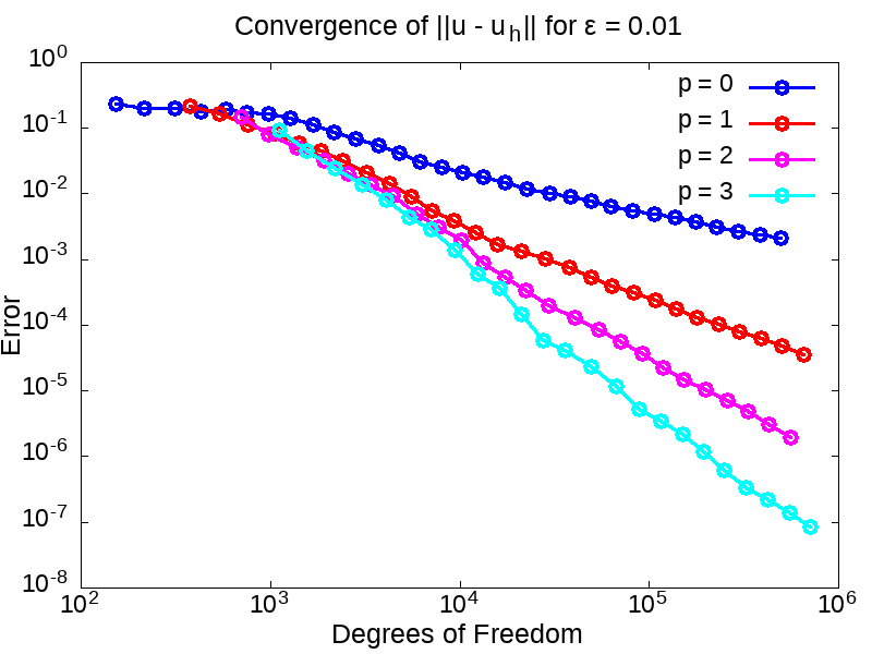
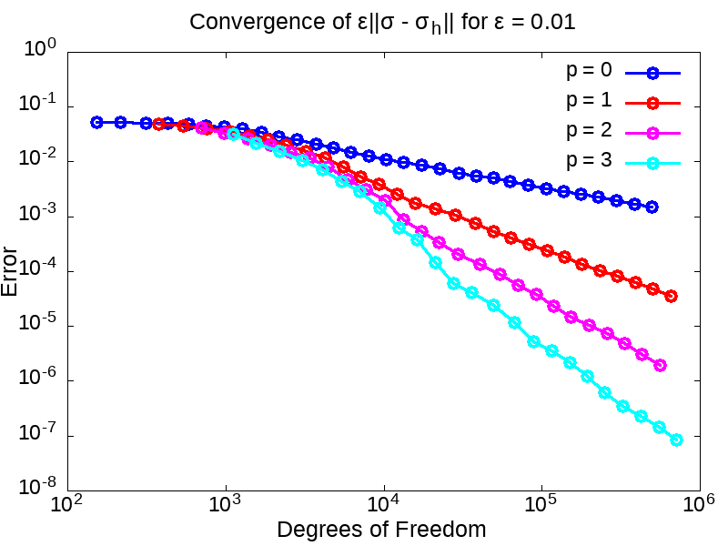
To begin, we run the adaptive algorithm driven by the a posteriori error estimator to around one million degrees of freedom for the diffusion coefficients and the polynomial degrees . We observe that the estimator , the solution error and the -scaled gradient error all converge with optimal order once the boundary has been sufficiently refined although we were unable to confirm this for due to reaching the asymptotic refinement regime only near the end of the computation. The convergence results for and the various different polynomial degrees are displayed in Figure 1.
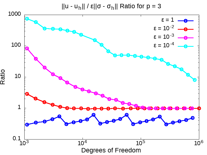
Next, we plot the ratio of the solution error to the -scaled gradient error in Figure 2 for and the different values of . Given that the scaling on these norms is the same relative scaling present in the trial norm (3.1) and that our test norm is designed for robustness in this trial norm, we expect that these two errors should be linked independently of . We do indeed observe this asymptotically; in fact, the ratio is an almost perfect value of one for and . In the preasymptotic regime, this ratio is large but the results are unreliable as the exact solution contains boundary layers meaning the error values, computed using quadrature, will not be accurate until the boundary layers are sufficiently refined.
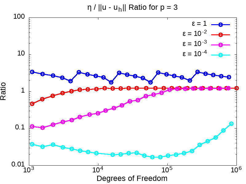
Although this is not the focus of the paper, for interest, we also plot the ratio of the error estimator to the solution error for and the different values in Figure 2. The results show that once the boundary has been sufficiently refined this ratio is one for and indicating asymptotic parity of the solution error and the estimator for this problem.
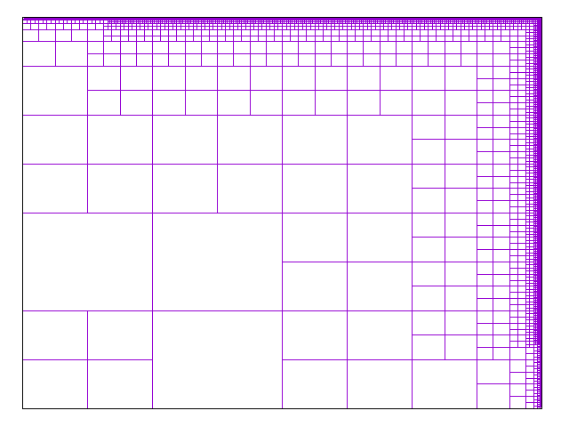
We display the grids from final runtime for and in Figure 3. The results show that our proposed test norm performs well for but for even the mesh-dependent modification made to the test norm is insufficient to stop unnecessary refinement around the inflow boundary in the pre-asymptotic regime despite no boundary layers being present.
5.2. Example 2
For this example, we consider the so-called Eriksson-Johnson model problem [18] thus we set , , and consider the following boundary conditions:
The solution to this problem has a boundary layer of width at the outflow boundary. Using separation of variables, this problem has the exact solution
where
and
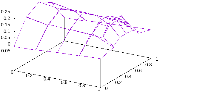
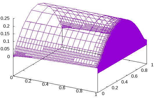
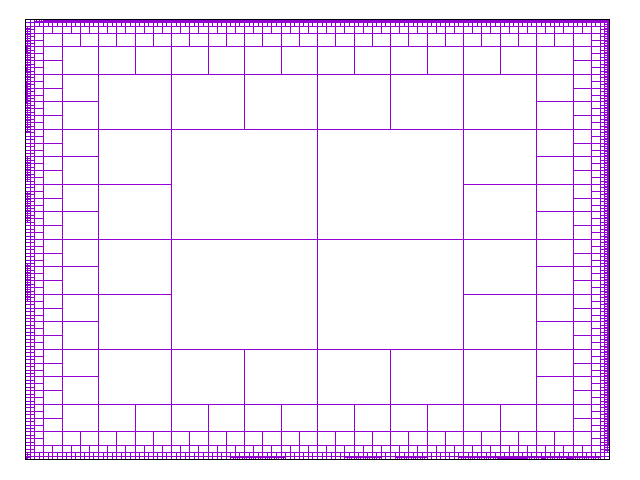
We will use the function for the inflow boundary condition. The numerical solution for and in the pre-asymptotic and asymptotic mesh refinement regimes is plotted in Figure 4. We see that the numerical solution is very stable even with barely any elements present and that, again, the estimator using our proposed test norm correctly picks up and refines the boundary layer.
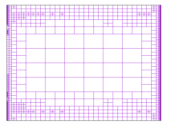
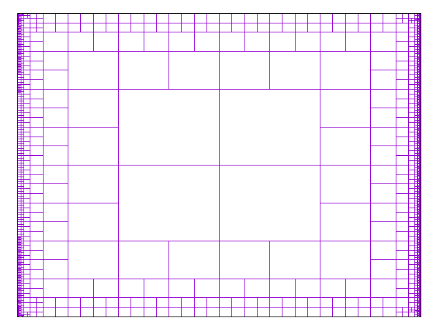
Next, we compare results for the adaptive algorithm as driven by our test norm versus the test norm from [8, 9]; in each case, adaptivity is driven by the respective test norm. For , we observe degeneration in mesh quality, plotted in Figure 5 (for = 3), for both test norms with extraneous refinement around the inflow boundary despite no layers present.
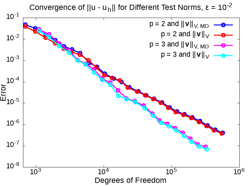
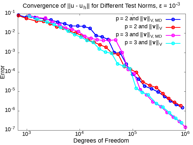
The solution errors for and , and under the two different test norms and are shown in Figure 6. The results show that our test norm performs slightly better for while the test norm performs better for although the difference in both cases is largely negligible indicating that, for this example, the two test norms perform more or less identically with respect to minimizing the solution error.
5.3. Example 3
Here, we select another example from [28]. We set and consider the non-constant convection . The Dirichlet boundary conditions and right-hand side are then chosen such that the solution to (1.1) is given by
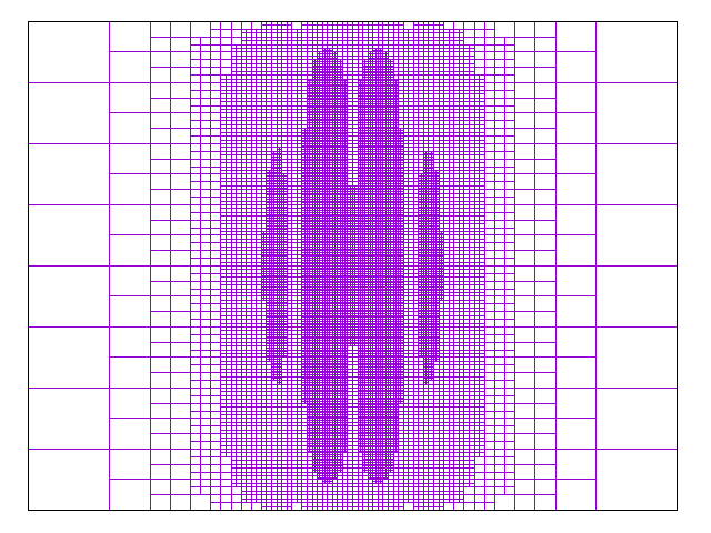
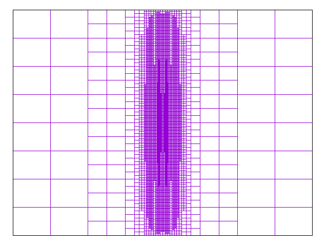
The solution to this problem exhibits an interior layer of width . Meshes for and are displayed in Figure 7 and clearly show that our test norm successfully picks up and refines the interior layer present in the solution.
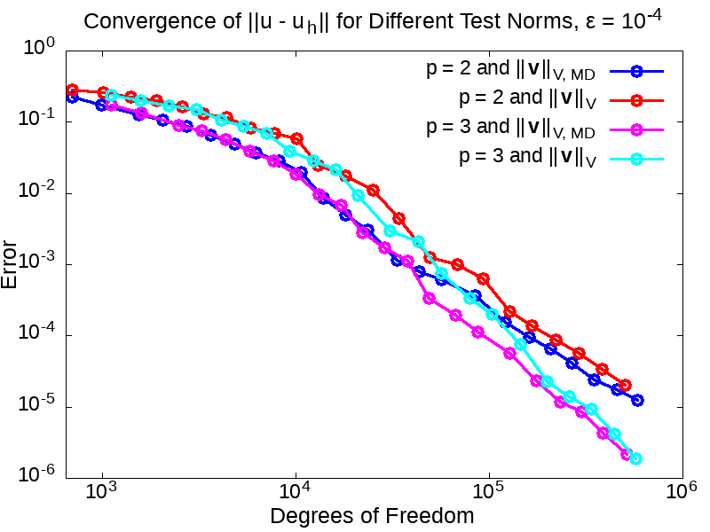
As in Example 2, we compare results for the adaptive algorithm as driven by our test norm versus the test norm from [8, 9]; in each case, adaptivity is driven by the respective test norm. The results given in Figure 8 show that solution errors under both test norms are robust with respect to . Our test norm outperforms the test norm for with the situation reversed for , however, both test norms deliver near identical values for the solution error once the mesh has been sufficiently refined.

6. Conclusions
We proposed the mesh-dependent quasi-optimal test norm
, for use in the DPG method based on the ultra-weak formulation of the convection-diffusion equation. We proved that this test norm is robust in the solution component and also robust in the gradient component once the mesh has been sufficiently refined; additionally, the proposed test norm was proven to have favorable scalings in the trace components. The robustness proof requires only minimal assumptions on the convection in contrast to similar results in the literature [8, 9].
Numerical experiments show that, when compared with the mesh-dependent test norm from [8, 9], our proposed test norm was competitive delivering near identical solution errors and producing similar meshes. The numerics imply that quasi-optimal test norms, when appropriately augmented with mesh-dependent terms and scaled with , can be competitive for the DPG method as applied to the convection-diffusion equation. Nevertheless, we believe that there is still much work to be done on this topic as none of the test norms in the literature (including our proposed test norm) performed well in all respects for .
References
- [1] Douglas N. Arnold, An interior penalty finite element method with discontinuous elements, SIAM journal on numerical analysis 19 (1982), no. 4, 742–760.
- [2] Wolfgang Bangerth, Ralf Hartmann, and Guido Kanschat, deal.II – a general-purpose object-oriented finite element library, ACM Transactions on Mathematical Software (TOMS) 33 (2007), no. 4, 24.
- [3] Carlos E. Baumann and John T. Oden, A discontinuous hp finite element method for convection—diffusion problems, Computer Methods in Applied Mechanics and Engineering 175 (1999), no. 3-4, 311–341.
- [4] Alexander N. Brooks and Thomas J. R. Hughes, A multidimensional upwind scheme with no crosswind diffusion, finite element methods for convection dominated flows, American Society of Mechanical Engineers, 1979.
- [5] by same author, Streamline upwind/Petrov-Galerkin formulations for convection dominated flows with particular emphasis on the incompressible Navier-Stokes equations, Computer methods in applied mechanics and engineering 32 (1982), no. 1-3, 199–259.
- [6] Andrea Cangiani, Emmanuil H. Georgoulis, and Stephen Metcalfe, Adaptive discontinuous Galerkin methods for nonstationary convection–diffusion problems, IMA Journal of Numerical Analysis 34 (2014), no. 4, 1578–1597.
- [7] Carsten Carstensen, Leszek Demkowicz, and Jay Gopalakrishnan, A posteriori error control for DPG methods, SIAM Journal on Numerical Analysis 52 (2014), no. 3, 1335–1353.
- [8] Jesse Chan, A DPG method for convection-diffusion problems, PhD Thesis, University of Texas (2013).
- [9] Jesse Chan, Norbert Heuer, Tan Bui-Thanh, and Leszek Demkowicz, A robust DPG method for convection-dominated diffusion problems II: Adjoint boundary conditions and mesh-dependent test norms, Computers & Mathematics with Applications 67 (2014), no. 4, 771–795.
- [10] Bernardo Cockburn, Bo Dong, Johnny Guzmán, Marco Restelli, and Riccardo Sacco, A hybridizable discontinuous Galerkin method for steady-state convection-diffusion-reaction problems, SIAM Journal on Scientific Computing 31 (2009), no. 5, 3827–3846.
- [11] Clint Dawson, Shuyu Sun, and Mary F. Wheeler, Compatible algorithms for coupled flow and transport, Computer Methods in Applied Mechanics and Engineering 193 (2004), no. 23-26, 2565–2580.
- [12] Leszek Demkowicz and Jay Gopalakrishnan, A class of discontinuous Petrov–Galerkin methods. II. Optimal test functions, Numerical Methods for Partial Differential Equations 27 (2011), no. 1, 70–105.
- [13] Leszek Demkowicz, Jay Gopalakrishnan, and Antti H. Niemi, A class of discontinuous Petrov–Galerkin methods. Part III: Adaptivity, Applied numerical mathematics 62 (2012), no. 4, 396–427.
- [14] Leszek Demkowicz and Jayadeep Gopalakrishnan, A class of discontinuous Petrov–Galerkin methods. Part I: The transport equation, Computer Methods in Applied Mechanics and Engineering 199 (2010), no. 23-24, 1558–1572.
- [15] by same author, Analysis of the DPG method for the Poisson equation, SIAM Journal on Numerical Analysis 49 (2011), no. 5, 1788–1809.
- [16] Leszek Demkowicz and Norbert Heuer, Robust DPG method for convection-dominated diffusion problems, SIAM Journal on Numerical Analysis 51 (2013), no. 5, 2514–2537.
- [17] Herbert Egger and Joachim Schöberl, A hybrid mixed discontinuous Galerkin finite-element method for convection–diffusion problems, IMA Journal of Numerical Analysis 30 (2010), no. 4, 1206–1234.
- [18] Kenneth Eriksson and Claes Johnson, Adaptive streamline diffusion finite element methods for stationary convection-diffusion problems, Mathematics of computation 60 (1993), no. 201, 167–188.
- [19] Juan C. Heinrich, Peter S. Huyakorn, Olgierd C. Zienkiewicz, and Andrew R. Mitchell, An ‘upwind’ finite element scheme for two-dimensional convective transport equation, International Journal for Numerical Methods in Engineering 11 (1977), no. 1, 131–143.
- [20] Ngoc C. Nguyen, Jaume Peraire, and Bernardo Cockburn, An implicit high-order hybridizable discontinuous Galerkin method for linear convection–diffusion equations, Journal of Computational Physics 228 (2009), no. 9, 3232–3254.
- [21] Antti H. Niemi, Nathaniel O. Collier, and Victor M. Calo, Discontinuous Petrov-Galerkin method based on the optimal test space norm for one-dimensional transport problems, Procedia Computer Science 4 (2011), 1862–1869.
- [22] by same author, Automatically stable discontinuous Petrov–Galerkin methods for stationary transport problems: Quasi-optimal test space norm, Computers & Mathematics with Applications 66 (2013), no. 10, 2096–2113.
- [23] Issei Oikawa, Hybridized discontinuous Galerkin method for convection–diffusion problems, Japan Journal of Industrial and Applied Mathematics 31 (2014), no. 2, 335–354.
- [24] Weifeng Qiu and Ke Shi, An HDG method for convection diffusion equation, Journal of Scientific Computing 66 (2016), no. 1, 346–357.
- [25] William H. Reed and Thomas R. Hill, Triangular mesh methods for the neutron transport equation, Tech. report, Los Alamos Scientific Lab., N. Mex.(USA), 1973.
- [26] Béatrice Rivière, Mary F. Wheeler, and Vivette Girault, Improved energy estimates for interior penalty, constrained and discontinuous Galerkin methods for elliptic problems. Part I, Computational Geosciences 3 (1999), no. 3-4, 337–360.
- [27] Jacob Salazar, Jaime Mora, and Leszek Demkowicz, Alternative enriched test spaces in the DPG method for singular perturbation problems, Computational Methods in Applied Mathematics 19 (2019), no. 3, 603–630.
- [28] Dominik Schötzau and Liang Zhu, A robust a-posteriori error estimator for discontinuous Galerkin methods for convection–diffusion equations, Applied numerical mathematics 59 (2009), no. 9, 2236–2255.
- [29] Jeff Zitelli, Ignacio Muga, Leszek Demkowicz, Jayadeep Gopalakrishnan, David Pardo, and Victor M. Calo, A class of discontinuous Petrov–Galerkin methods. Part IV: The optimal test norm and time-harmonic wave propagation in 1D, Journal of Computational Physics 230 (2011), no. 7, 2406–2432.